Positive-Unlabeled Constraint Learning (PUCL) for Inferring Nonlinear Continuous Constraints Functions from Expert Demonstrations

Abstract

Planning for a wide range of real-world robotic tasks necessitates to know and write all constraints. However, instances exist where these constraints are either unknown or challenging to specify accurately. A possible solution is to infer the unknown constraints from expert demonstration. This paper presents a novel Positive-Unlabeled Constraint Learning (PUCL) algorithm to infer a continuous arbitrary constraint function from demonstration, without requiring prior knowledge of the true constraint parameterization or environmental model as existing works. Within our framework, we treat all data in demonstrations as positive (feasible) data, and learn a control policy to generate potentially infeasible trajectories, which serve as unlabeled data. In each iteration, we first update the policy and then a two-step positive-unlabeled learning procedure is applied, where it first identifies reliable infeasible data using a distance metric, and secondly learns a binary feasibility classifier (i.e., constraint function) from the feasible demonstrations and reliable infeasible data. The proposed framework is flexible to learn complex-shaped constraint boundary and will not mistakenly classify demonstrations as infeasible as previous methods. The effectiveness of the proposed method is verified in three robotic tasks, using a networked policy or a dynamical system policy. It successfully infers and transfers the continuous nonlinear constraints and outperforms other baseline methods in terms of constraint accuracy and policy safety.

I Introduction

Planning for many robotics and automation tasks requires explicit knowledge of constraints, which define what states or trajectories are allowed or must be avoided [1, 2]. Sometimes these constraints are initially unknown or hard to specify mathematically, especially when they are nonlinear, possess unknown shape of boundary or are inherent to user’s preference and experience. For example, human users may determine an implicit minimum distance of the robot to obstacles based on the material of the obstacle (glass or metal), the shape and density of obstacles and their own personal preference. The robot should be able to infer such a constraint as well as the desired minimum distance to achieve the task goal and meet human’s requirements. This means an explicit constraint should be inferred somehow, e.g., from existing human demonstration sets.

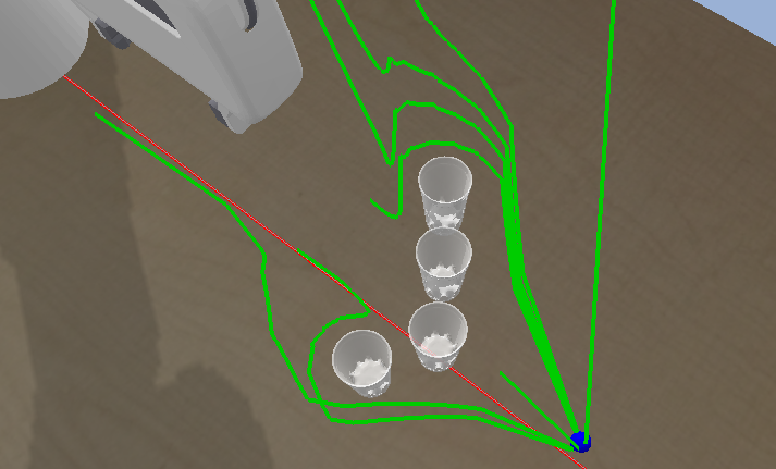
(a) Demonstrations

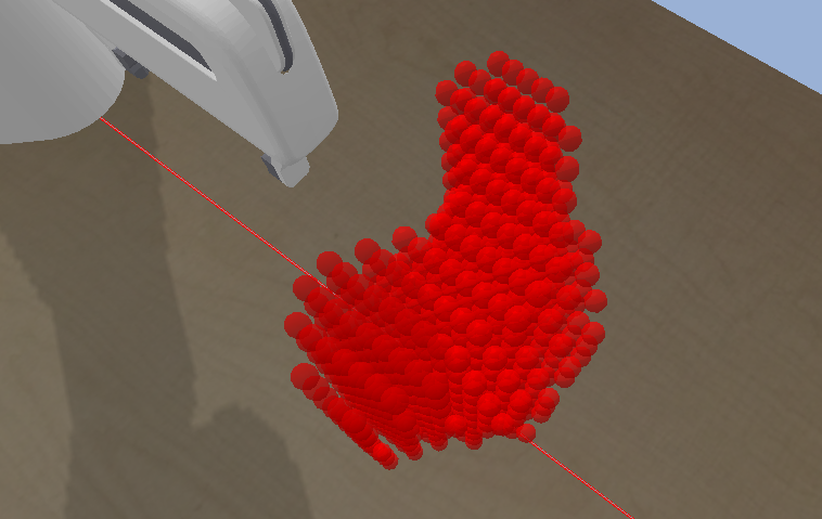
(b) Learned constraint

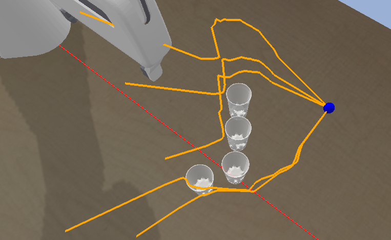
(c) Transferred policy

Figure 1: The task requires the robot to reach a target state (blue dot) while avoid going close to or over the cups. These unknown constraints can be translated into an infeasible region that must be inferred from a set of feasible paths demonstrated by an expert (in green). (a) Demonstrations (shown in green lines). (b) Learned constraint region (in red) (c) New transferred policy (in orange), generated by transferring the learned constraint to a similar task of reaching another target state (blue dot) from different starting points.

Constraint inference from demonstrations has drawn more and more attention since 2018 [3]. Various methods have been developed to learn various types of constraints. In this work, we focus on the constraints of not visiting some undesired states(-actions) throughout the trajectory (discussed in detail in section II-A). These constraints define what the user does not want to happen and are ubiquitous in practice, e.g., not crashing into an unknown obstacle or not surpassing an unknown maximum velocity.

Existing constraint learning methods can be roughly divided into inverse reinforcement learning (IRL)-based methods and mixed-integer-programming (MIP)-based methods.

IRL-based methods draw inspiration from the concepts and approaches of IRL and adapt them to learn the constraint function. [4] first formulate the constraint learning problem in the maximum likelihood inference framework. They introduce a Boltzmann policy model, where the likelihood of any feasible trajectory is assumed to be proportional to the exponential return of the trajectory, while the likelihood of any infeasible trajectory is 0. Then a greedy algorithm is proposed to add the smallest number of infeasible states that maximize the likelihood of the demonstrations. Further, [5] and [6] extend the maximum entropy framework from a deterministic setting into a stochastic setting, with soft or probabilistic constraints. [7] proposes an algorithm that learns a neural network policy via deep RL and generates high return trajectories with the policy network. Then the infeasible states are again added based on the maximum likelihood principle. [8] proposes Maximum Entropy Constraint Learning (MECL) algorithm. It not only approximates the policy with a network but also learns a constraint network, which is optimized by making a gradient ascent on the maximum likelihood objective function. More recently, [9] proposes a variational approach to infer the distribution of constraint and capture the epistemic uncertainty. However, despite the success of aforementioned IRL-based methods, they suffer from the two problems: theoretically, their maximum likelihood loss function optimizes all states visited by the policy to be infeasible, and at the same time optimizes states visited by the demonstrations to be feasible. If the demonstrations and policy overlap a lot, this loss will lead to conflicting updating, slowing the training and prone to classifying safe demonstrated states as infeasible. In addition to that, in practice their methods are mostly applied to recover linear constraints of a single state element, e.g. $x\geq-3$ [8, 9, 10], and, as we show later in the paper, perform relatively poorly in learning more complex constraints.

In parallel, another line of research based on MIP has been developed. [3] first studies how to infer infeasible states from a demonstration set in a grid world. They assume that all possible trajectories that could earn higher rewards than the demonstration must be constrained in some way, or the expert could have passed those trajectories. In practice, they use hit-and-run sampling to obtain such higher-reward trajectories and solve an integer program to recover the constrained states in a grid world. This MIP method is soon extended to continuous state space and parameterized continuous constraint functions, where the constraint is represented as unions and intersections of axis-aligned box [11]. Later, the same author proposes to leverage the closed-form environmental model and the KKT optimality condition to infer the parameters of a known constraint parameterization [11], or a Gaussian Process constraint model [12]. However, these MPI-based methods either require the full knowledge of a differentiable model of the environment and agent [11, 12], which is not always available in practice , or can only learn constrained region expressed with unions and intersections of box [13].

In summary, despite these impressive advances, it still remains to be shown how to learn continuous nonlinear constraint functions from a small sample of demonstrations, without full knowledge of true constraint parameterization and environmental model. To overcome the aforementioned challenge, we propose a two-step Positive-Unlabeled Constraint Learning (PUCL) method, inspired by a machine learning subarea Positive-Unlabeled (PU) learning [14] and extended from our previous work [15]. Within our framework, we treat all data in demonstrations as positive (feasible) dataset, and learn a policy to generate many potentially unsafe trajectories which serve as unlabeled data with unknown feasibility. Then a two-step PU learning technique is applied, where we first identify reliable infeasible data and secondly learn a binary feasibility classifier (i.e., constraint function) from the positive data and reliable infeasible data. The proposed method is flexible to learn complex-shaped constraint boundary without the need to know the true constraint parameterization. It also avoids the drawback of IRL-based method that mistakenly optimize and classify demonstrations as infeasible, thus improving the performance and accuracy.

The idea and approach of positive-unlabeled constraint learning was first explored in our previous work [15]. This work replaced the postprocessing approach in [15] with a more powerful two-step approach and solved more complex constraint learning tasks.

II Preliminaries and Problem Statements

II-A Preliminaries

For a finite-horizon Markov decision process (MDP) [16, 17], states and actions are denoted by $s\in\mathcal{S}$ and $a\in\mathcal{A}$. $\gamma$ denotes the discount factor, and the potentially unknown real-valued reward is denoted by $r(s,a)$. A trajectory $\tau=\{s_{1},a_{1},\ldots,s_{T},a_{T}\}$ contains a sequence of state-action pairs in one episode. For the trajectory $\tau$, the total discounted reward (return) is defined as $r(\tau)=\sum_{t=1}^{T}\gamma^{t}r(s_{t},a_{t})$. A policy, the mapping between states and actions, is denoted by $a=\pi(s)$.

In this study, we focus on learning the Markovian state-action constraints, i.e., avoiding visiting some forbidden states (and actions) throughout the entire trajectory. Mathematically, we denote the true constraint set by $\mathcal{C^{*}}=\{(s,a)\in\mathcal{S}\times\mathcal{A}|(s,a)\text{ is truly infeasible}\}$. Thus, the true constraint is written as $(s,a)\notin\mathcal{C^{*}}$. This definition implicitly assumes that the studied constraint is (1) time-independent: the infeasible set remains unchanged for every timestep of every trajectory; (2) deterministic: a state-action pair is either truly feasible or truly infeasible, though the prediction model could output a probabilistic prediction of feasibility. (3) defined only on the current state (and potentially action), independent of previous states and actions. In addition to the unknown constraints, some known constraints could also be present in the task, e.g., goal state constraints and system dynamic constraints. For simplicity of explanation, all demonstrations and trajectories are assumed to satisfy the known constraints (trajectories violating known constraints are discarded and not used for inferring unknown constraint).

II-B Problem Formulation

As in similar works [8, 3], we require that the reward function $r(s,a)$ is known in advance. This assumption is reasonable in many robotics applications, where the reward might be shortest path, shortest time to reach the goal. We emphasize that the unknown constraints are not indicated in the known reward function, i.e., the agent does not receive any penalty for violating the unknown constraints. Subsequently, the real task is written as a constrained optimization problem:

Problem 1 (Constrained optimization problem)

$$\max_{\{a_{i}\sim\pi\}^{T}_{i=0}} \quad r(\tau)$$ (1a)

s.t. $$\quad(s_{i},a_{i})\notin\mathcal{C^{*}},\quad\forall(s_{i},a_{i})\in\tau$$ (1b)

where $r(\tau)$ represents the reward function of trajectory $\tau$, (1b) represents the unknown constraint to be learned.

The demonstration set $\mathcal{D}=\{\tau_{i}\}^{M_{d}}_{i=1}$ comprises trajectories demonstrated by a demonstrator, who may not necessarily be an expert but still to some extent solves the task. More concretely, we make the following assumption of the demonstrations optimality and feasibility:

Assumption 1 (Demonstrations Sub-optimality and Feasibility).

Any demonstration $\tau_{i}^{d}$ from $\mathcal{D}=\{\tau_{i}^{d}\}^{M_{d}}_{i=1}$ is feasible and $\delta$-sub-optimal solution to the problem 1:

1. (feasible): $\tau_{i}^{d}$ satisfies (1b) and all known constraints.

2. ($\delta$-sub-optimal): $(1-\delta)r(\tau^{*})\leq r(\tau_{i})$, where $\tau^{*}$ is the feasible optimal solution to the problem 1. $\delta\in[0,1)$ is a coefficient of sub-optimality. In practice it is treated as a hyper-parameter and specified according to the user’s confidence of demonstration optimality.

We formally define the constraint learning task as:

Definition 1 (Constraint Learning).

The task of learning constraint from demonstration is to recover the unknown true constraint set $C^{*}$ in Problem 1 from the demonstration set $\mathcal{D}$, with the known reward function $r(\tau)$.

Note that in the rest of the paper we only consider the state constraints and omit actions, but the framework can be easily extended to state-action constraints by augmenting the state with the action to form an augmented state.

To represent and learn an arbitrary constraint set in continuous space, we approximate it with a constraint network $\zeta_{\theta}(s)\in(0,1)$, which induces a constraint set $\mathcal{C}_{\theta}=\{s\in\mathcal{S}|\zeta_{\theta}(s)\leq d\}$, where $\theta$ is the network weights and $d=0.5$ is the threshold.

III Method

III-A Motivation: Constraint Inference as Positive-Unlabeled Learning

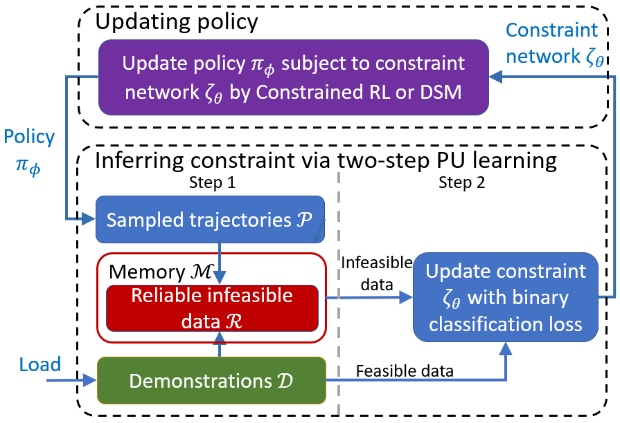
Figure 2: The framework of the proposed constraint learning algorithm PUCL. It alternates between updating policy using current constraint network, and inferring constraint from demonstrations and current policy. The constraint is inferred using a novel two-step positive-unlabeled learning technique. In the first step, the trajectories $\mathcal{P}$ sampled from current policy are viewed as unlabeled data, while the demonstrations are viewed as labeled feasible data. From the two datasets we identify reliable infeasible data using a distance-based metric. In the second step, the reliable infeasible data from current iteration and previous iterations, as well as the feasible demonstrations, are used to train a constraint network using a standard binary classification loss.

As in many IRL-based and MBI-based works [8, 3], we infer the underlying constraint by contrasting the (safe) demonstration with some potentially unsafe trajectories generated by a certain policy. The training follows an iterative framework to incrementally learn the constraint. In each iteration, we first sample a set of high-reward trajectories $\mathcal{P}=\{\tau_{i}\}^{M_{p}}_{i=1}$ by performing the current policy $\pi_{\phi}$ (discussed later in III-D). Each sampled trajectory consists of sequential state-action pairs $\tau=\{s_{j},a_{j}\}_{j=1}^{N_{i}}$. Similar to [3], we speculate that the trajectory which wins higher reward than demonstration is potentially unsafe and cheat by visiting some forbidden states. However, it remains unclear which specific state(s) within the trajectory are unsafe. In other words, trajectory $\tau$ visits both truly feasible states and truly infeasible states but both remain unlabeled. In contrast, it is certain that all states on the demonstrated trajectories are labeled feasible by Assumption 1. Our goal is to classify each single state as feasible or infeasible by learning from a batch of fully labeled feasible samples and another batch of unlabeled mixed samples.

This insight inspires us to formulate constraint inference as a positive-unlabeled learning problem. PU learning is a machine learning technique that aims to learn a classifier from a positive dataset and an unlabeled dataset containing both positive and negative samples [14]. Within our framework, positive samples correspond to feasible states. Thus, the data from demonstrations serve as positive data, while the policy offers unlabeled data containing some infeasible samples. We can thus utilize PU learning methods to uncover the infeasible states from the two datasets.

PU learning methods for binary classification mainly divide into three categories: two-step methods, biased learning and class-prior-based methods [14]. The latter two methods both rely on an important assumption, Sampled Completely At Random (SCAR), which requires the demonstrations and policy to have a similar distribution in the truly feasible region. Our former paper [15] already explored the class-prior-based methods. However, the required SCAR assumption is usually unrealistic since the state distribution largely depends on the specific task and is hard to control. Violation of this assumption leads to performance degradation. In contrast, the two-step methods are based on a separability assumption, which requires the two classes can be strictly separated. Since we limit our discussion to deterministic constraint and a state is either truly feasible or infeasible, the separability assumption naturally holds. Therefore, we develop our methods based on the two-step framework [18, 19].

III-B Method: Positive-Unlabeled Constraint Learning

Our two-step PU learning methods consists of the following steps: (1) identifying reliable infeasible states from unlabeled trajectory set $\mathcal{P}$, and (2) using supervised learning techniques to learn a classifier from the feasible demonstrations $\mathcal{D}$ and reliable infeasible state set (denoted as $\mathcal{R}$). In step 1, the identification of $\mathcal{R}$ starts from the intuition that the states in the unlabeled set $\mathcal{P}$ that are very different from all states in the demonstration set $\mathcal{D}$ are highly likely to be truly infeasible. We propose a kNN-like approach, which is straightforward to comprehend and implement, to identify the reliable infeasible set $\mathcal{R}$. The unlabeled states are first ranked according to their distance to the $k$ nearest feasible states from demonstration set. The unlabeled states whose distance is higher than a threshold are selected as reliable infeasible states. Mathematically, the ranking score for each unlabeled data $s\in\tau_{i}\in\mathcal{P}$ is calculated by the average distance:

$$S_{\mathcal{D}}(s)=\frac{1}{k}\sum_{s^{\prime}\in kNN(s,\mathcal{D})}dis(s,s^{\prime})$$ (2)

where $kNN(s,\mathcal{D})$ indicates the $k$-nearest neighbours of $s$ in the set $\mathcal{D}$, and $dis(s,s^{\prime})$ is a distance metric selected based on the specific task. In this work, this distance is always measured using Euclidean distance. Additionally, considering the range of each dimension of the state could be very different, each dimension is preferred to be normalized before computing distance and nearest neighbours. The reliable infeasible set $\mathcal{R}$ consists of all unlabeled data whose score exceeds a threshold $d_{r}$.

$$\mathcal{R}=\{s\in\mathcal{P}|S_{\mathcal{D}}(s)\geq d_{r}\}$$ (3)

In practice, since $\mathcal{D}$ contains consecutive state series from trajectories, a smaller $k$ around 1-5 is preferred. For $d_{r}$, it indicates user’s belief over the size of true infeasible area. A lower $d_{r}$ tends to identify a larger $\mathcal{R}$, leading to a more conservative constraint network. Conversely, a higher $d_{r}$ tends to find a smaller $\mathcal{R}$ and a more radical constraint function. In the extreme case of $d_{r}=0$, nearly any state not visited by the demonstrations is classified as infeasible. We admit selecting $d_{r}$ can be tricky, but such a parameter is generally inevitable since learning constraints is known to be an ill-posed problem with infinite valid solutions [8].

However, in the case where the demonstration closely adheres to the true constraint boundary with a distance shorter than $d_{r}$, kNN-like metric may fail to learn an accurate boundary, as the reliable infeasible data are all at least $d_{r}$ far from the demonstrations. To adapt to this case, we additionally expand $\mathcal{R}$ by adding the state(s) from each trajectory in $\mathcal{P}$ that is closest to the original $\mathcal{R}$, since these states are likely to between the current boudnary and the true boudnary.

$$\mathcal{R}\leftarrow\mathcal{R}\cup\{s|\exists\tau_{i}\in\mathcal{P},s=\arg\min_{s\in\tau_{i}}S_{\mathcal{R}}(s)\}$$ (4)

where $S_{\mathcal{R}}(s)$ is the score function sharing similar definition as $S_{\mathcal{D}}(s)$ in (2) but with a different set $\mathcal{P}$.

In step 2, we directly train a neural network binary classifier $\zeta_{\theta}(s)$ from the reliable infeasible data $\mathcal{R}$, the memory buffer $\mathcal{M}$ (discussed later in III-C) and the (feasible) demonstrations data $\mathcal{D}$ with a standard cross entropy loss:

$$\mathcal{L}(\theta)=-\frac{1}{N+M}[\sum^{N}_{s_{i}\sim\mathcal{D}}\log\zeta_{\theta}(s_{i})-\sum^{M}_{s_{j}\sim\mathcal{R}\cup\mathcal{M}}\log(1-\zeta_{\theta}(s_{j}))]$$ (5)

After training, the learned constraint set is expressed as $\mathcal{C}_{\theta}=\{s\in\mathcal{S}|\zeta_{\theta}(s)\leq 0.5\}$.

III-C Iterative Learning Framework with Policy Filter and Memory Buffer

Last subsection discussed about learning constraint from a given unsafe set $\mathcal{P}$ as well as demonstrations $\mathcal{D}$. This and next subsection will elaborate on the generation of unsafe set $\mathcal{P}$. Existing methods generate $\mathcal{P}$ either in an iterative manner [8, 4, 9] or in a one-batch manner [3, 13, 7]. The former iteratively updates policy with current constraint function and generate new trajectories $\mathcal{P}$ to update the constraint. Since the policy is always updated with respect to up-to-date constraint network, the new trajectories generated in each iteration are mostly distributed around the boundary of the current constraint network, which will improve the accuracy of the constraint boundary. Therefore, this manner is efficient to learn the constraint boundary and can automatically adjust the distribution of the generated trajectories.

In contrast, the one-batch manner generates a bulk of trajectories $\mathcal{P}$ uniformly[3] or greedily[7] at the start of training. The following training only takes place on only existing $\mathcal{P}$, with no new data generated. This manner is more stable but relatively inefficient and poses a higher demand on the diversity and the coverage of the generated trajectories.

This work follows the iterative framework, and introduce a policy filter and a memory buffer both from our previous work [15]. Fig. 2 gives a sketch of the whole iterative structure.

Policy filter: In each iteration of policy updating, the policy is updated for fixed steps with the current constraint network $\zeta(s;\theta)$. To prevent bad updates from bad policies, a policy filter (6) is introduced to select trajectories with relatively high reward than the demonstration, which are believed to truly violate the unknown constraint according to Assumption 1.

$$\mathcal{P}\leftarrow\{\tau_{i}\in\mathcal{P}|r(\tau_{i})\geq(1-\delta)r(\tau_{i}^{\mathcal{D}})\}$$ (6)

where $\delta$ is a coefficient defined in Assumption 1, $\tau_{i}^{\mathcal{D}}$ is the demonstration that starts from the same state as $\tau_{i}$.

Memory buffer: Most iterative-framework-based papers generate new trajectories in each iteration and discard those from previous iterations [8, 4, 9]. Our previous work [15] identified that such a training manner tends to forget the infeasible region learned in early iterations. Thus, we introduce a memory replay buffer and record all the reliable infeasible data $\mathcal{R}$ identified in each iteration into the memory buffer $\mathcal{M}$. In the following iterations of learning constraints, both the current $\mathcal{R}$ and memory buffer $\mathcal{M}$ serve as infeasible data for training (see (5)).

III-D Represent and Learn Policy via Constrained RL or Dynamical System Modulation

In the iterative framework discussed in the last subsection, we need to maintain a policy to generates high-reward trajectories while satisfying the currently learned constraints. We consider and compare two approaches: 1) constrained RL, which is effective at learning constrained policies in a high-dimensional environment with complex reward function but suffers from a slow and unstable training process[20], and 2) dynamical system modulation (DSM), which modulates a nominal policy with a rotation matrix to satisfy safety constraints. It features minimal training time and provides a controller with stability guarantee. This method is applicable and very suitable for robotic tasks where the control command is the velocity of each state (i.e., joint angle or end-effector pose).

Constrained reinforcement learning: a networked policy is trained with a modern constrained RL algorithm PID-Lagrangian[20], which offers the advantage of automatically and more stably adjusting the penalty weight. As shown in (7), it reshapes the original reward by incorporating the constraint as a penalty term into the original reward function to avoid the infeasible states. Here, $w_{p}$ is a penalty weight adjusted by PID-Lagrangian updating rules [20, 21, 22], and $c(s)$ is the constraint indicator function.

Using this reshaped $r^{\prime}(s,a)$, a constrained optimal policy can be straightforwardly learned with the standard RL algorithm PPO [23].

$$r^{\prime}(s,a)=r(s,a)-w_{p}c_{\theta}(s),\quad\text{where}$$ (7)

$$c_{\theta}(s)=\begin{cases}0&\text{if $\zeta_{\theta}(s)>d$ (feasible)}\\ 1&\text{if $\zeta_{\theta}(s)\leq d$ (infeasible)}\\ \end{cases}$$

Dynamical System Modulation: For the task where the control input is the velocity or acceleration of each state dimension, DSM can be applied to obtain a safe control policy by modulating nominal policy with the constraint network. The nominal dynamical system policy is represented as (8), where $s_{g}$ is the goal state and matrix $A(s)$ is a Gaussian Mixture Regression model learned from the known reward function following [24].

$$\pi(s)=\dot{s}=A(s)(s-s_{g})$$ (8)

Given a learned constraint network $\zeta(s;\theta)$ whose output ranges from 0 to 1, one can obtain a provably safe policy $\pi(s;\zeta)$ by modulating the nominal policy following (9) [25], where $n(s)$ is the normal vector to the constraint boundary, $e_{i}(s)$ are the tangent vectors, $r(s)$ is the vector towards a reference point, $\lambda_{i}(s)$ modify the velocity along different vectors, and $\Gamma(s)$ specifies the relative distance of current state $s$ to the constraint boundary.

$$\pi(s)=M(s)A(s)(s-s_{g}),\quad\text{where}$$ (9a)

$$M(s)=E(s)D(s)E^{-1}(s),$$ (9b)

$$E(s)=[r(s),e_{1}(s),e_{2}(s),...e_{n-1}(s)],$$ (9c)

$$n(s)=\frac{d\zeta(s)}{ds},n(s)\perp e_{1}(s)\perp e_{2}(s)\perp...e_{n-1}(s)$$ (9d)

$$D(s)=diag[\lambda_{1}(s),\lambda_{2}(s),\lambda_{3}(s)...,\lambda_{n}(s)],$$ (9e)

$$\lambda_{1}(s)=1-\frac{1}{\Gamma(s)},\lambda_{2,3,...,n}(s)=1+\frac{1}{\Gamma(s)},$$ (9f)

$$\Gamma(s)=1+10*(\zeta(s)-0.5)^{0.2}$$ (9g)

Finally, the pseudo-code for the algorithm is given in Algorithm 1.

Algorithm 1 Positive-Unlabeled Constraint Learning (PUCL)

1:  input: Demonstration set $\mathcal{D}$, randomly initialized constraint network $\zeta_{\theta}$, randomly initialized policy network $\pi_{\phi}$, empty memory buffer $\mathcal{M}=\varnothing$

2:  repeat

3:     Update the policy $\pi_{\phi}$ with the reshaped reward (7) and the current constraint network $\zeta_{\theta}$ using constrained RL or DS modulation

4:     Sample trajectory set $\mathcal{P}$ using the current policy $\pi_{\phi}$ from the same starting points as each demonstration

5:     Filter sampled set $\mathcal{P}$ with (6): $\mathcal{P}\leftarrow\{\tau_{i}\in\mathcal{P}|r(\tau_{i})\geq(1-\delta)r(\tau_{i}^{\mathcal{D}})\}$

6:     Identify and expand reliable infeasible set $\mathcal{R}$ using metric (3) and (4) $\mathcal{R}=\{s\in\mathcal{P}|S_{\mathcal{D}}(s)\geq d_{r}\}$ $\mathcal{R}\leftarrow\mathcal{R}\cup\{s|\exists\tau_{i}\in\mathcal{P},s=\arg\min_{s\in\tau_{i}}S_{\mathcal{R}}(s)\}$

7:     Train the constraint network $\zeta_{\theta}$ with the demonstration $\mathcal{D}$, reliable infeasible set $\mathcal{R}$ and memory buffer $\mathcal{M}$ $\mathcal{L}(\theta)=-\frac{1}{N+M}[\sum^{N}_{s_{i}\sim\mathcal{D}}\log\zeta_{\theta}(s_{i})-\sum^{M}_{s_{j}\sim\mathcal{R}\cup\mathcal{M}}\log(1-\zeta_{\theta}(s_{j}))]$

8:     Save all data from $\mathcal{R}$ into the memory buffer $\mathcal{M}\leftarrow\mathcal{M}\cup\mathcal{R}$

9:  until meet some stop criterion

IV Experiment

IV-A Experiment Setup

Environment and constraint: to examine the performance of the proposed method, we apply it to learn two position constraints of the end-effector’s trajectory of a Panda robot arm, one in 2D and another in 3D spaces. In both tasks, the agent is initialized randomly and rewarded to reach a goal state. The state space consists of 2D or 3D positions of the end-effector and the control variables are their corresponding velocities. In the 2D reaching task, the true constraint is avoiding an irregular obstacle composed of 2 ellipses as shown in Fig. 3. In the 3D reaching task, the true constraint is avoiding tall cylinder(s).

We emphasize that learning these two constraints is nontrivial and challenging in our problem setting for several reasons. Firstly, we assume no prior knowledge of the obstacles’ size, shape, and location, nor of the true constraints, while some existing methods learn constraints of obstacles with known shape (i.e., a box or a cylinder) [13]. Secondly, there is no requirement for a differentiable environmental model (if using constrained RL to learn policy). Thirdly, the constraints are nonlinear, not just (the union of) boxes or hyperplanes, which contrasts with previous IRL-based constraint learning works that only learn a linear plain constraint such as $x\geq-3$ [8, 9].

The expert demonstration sets for two tasks consists of 4 or 10 safe trajectories, respectively. All demonstrations are generated by an entropy-regularized suboptimal RL agent, trained assuming full knowledge of the true constraint. The reward function in both tasks are the negative of the Cartesian path length to reach the goal, which is a natural choice for a goal-reaching task.

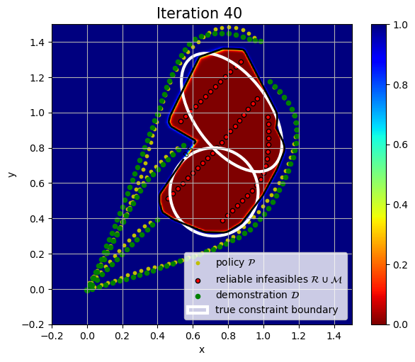
(a) PUCL (ours)

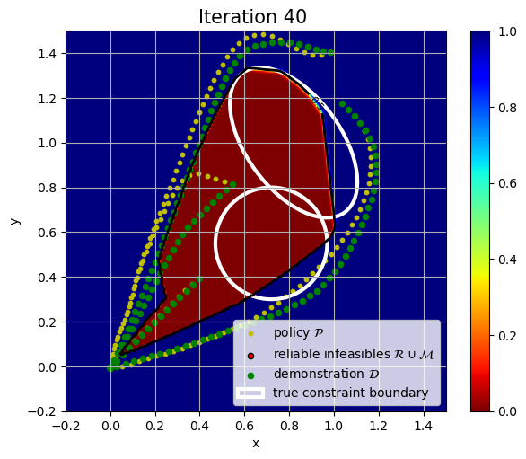
(b) MECL

Figure 3: True constraint and constraint learned with the proposed method PUCL and baseline MECL [8] in the 2D reaching task. The two white ellipses represent the boundary of the true constraint. The heat map is a visualization of the learned constraint $\zeta_{\theta}$, where the red region of $\zeta=0$ represents infeasibility, while the blue regions of $\zeta=1$ indicate feasibility. The trajectories of the demonstrations and the policy are shown in green and yellow, respectively. The red points correspond to identified reliable infeasible data $\mathcal{R}\cup\mathcal{M}$ (only for PUCL).

Baselines and implementations: Our baselines are chosen to study the following two questions:

1. How effective is our PUCL method compared with other constraint learning algorithms with similar problem setting?

2. In our PUCL framework, what are the differences between using constrained RL and dynamical system modulation to obtain the policy?

To answer question 1, we compare the constraint learning performance of the four methods, all using constrained RL as the policy: 1) PUCL (the proposed method); 2) maximum-likelihood constraint learning (MECL) [8], a popular IRL-based method that can learn a continuous arbitrary constraint function; 3) binary classifier (BC) [8], a method directly trains an NN feasibility classifier using loss (5) but with all data from $\mathcal{P}$ as infeasible data; 4) generative-PUCL (GPUCL), an alternative PUCL approach using a generative model to identify reliable infeasible data. It first learns a Gaussian Mixture Model (GMM) of the expert distribution, and then identifies reliable infeasible data as the data from $\mathcal{P}$ with the lowest likelihood of being generated by the GMM. GPUCL is also first formulated in this paper but do not discussed in detail due to weaker performance. The results of comparison of the above four methods are presented in section IV-B.

To answer question 2, we conduct another experiment implementing our PUCL approach using 1) a constrained RL policy or 2) a DSM policy (see section III-D). The two frameworks are named CRL-PUCL and DSM-PUCL, respectively, and the results of comparison are presented in section IV-C.

A list of important hyperparameters of our algorithm is given in Table I. The hidden activation functions in all networks are Leaky ReLU. The output activation function of the constraint network is the sigmoid function, whereas that of the policy and value network is tanh. Other baselines all adopt the same network architecture. Please refer to our code repo (released later) for other parameters.

TABLE I: List of hyperparameters of PUCL. For the neural network architectures, the number of hidden units in each layer is mentioned.

	2D task	3D task
Policy Network	64, 64	64, 64
Value Network	64, 64	64, 64
Constraint Network	32, 32	32, 32
Policy Learning Rate	$3\times 10^{-4}$	$3\times 10^{-4}$
Constraint Learning Rate	$5\times 10^{-3}$	$5\times 10^{-3}$
PID-Lagrangian $K_{p}$	1	20
PID-Lagrangian $K_{i}$	0.1	0.5
$\mathcal{R}$ identification threshold $d_{r}$	0.12	0.03
$\mathcal{R}$ identification $k$	1	1
sub-optimal coefficient $\delta$	0	0.03

Metrics: we present the evaluation utilizing two metrics: 1) the IoU (the intersection over union) index, which measures the correctness of the learned constraints. We uniformly sample points in the state space, and compute IoU as (Number of points which are both predicted to be infeasible and truly infeasible) divided by (Number of points either predicted to be infeasible or truly infeasible); 2) the unsafe rate, the per-step true constraint violation rate of the policy learned/modulated from the learned constraint.

(a) IoU - 2D task

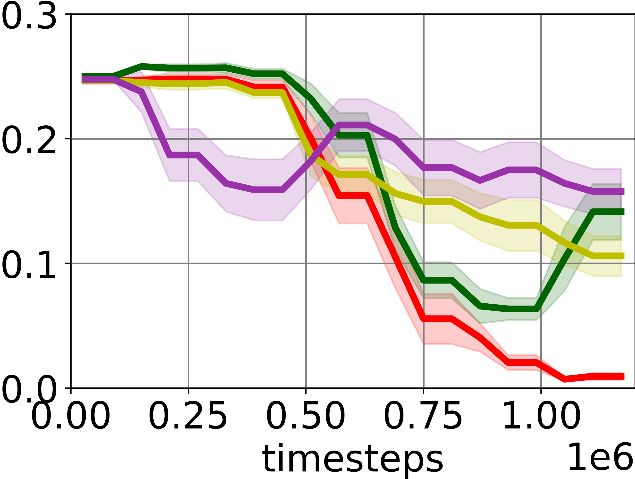
(b) Unsafe rate - 2D task

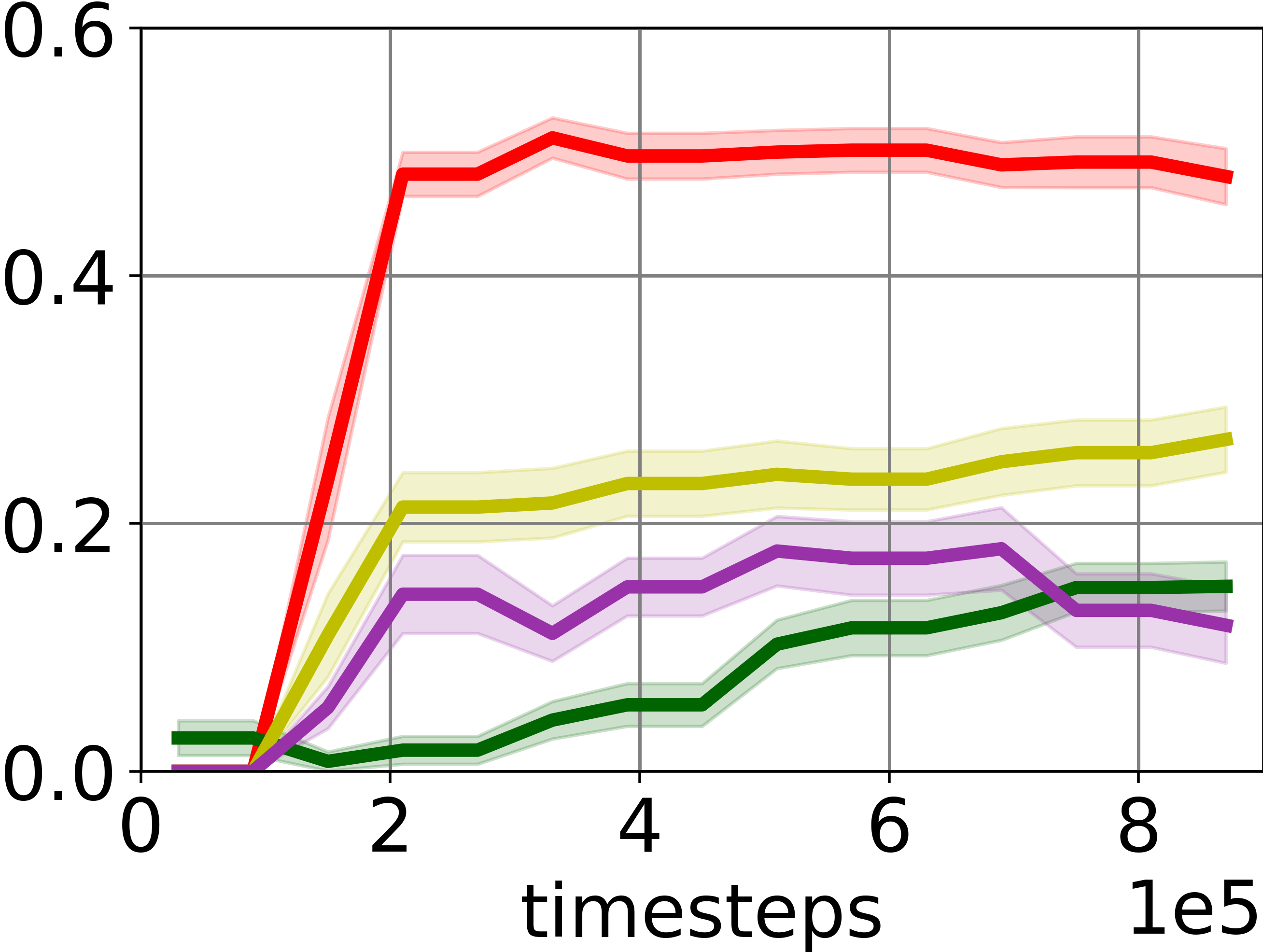
(c) IoU - 3D task

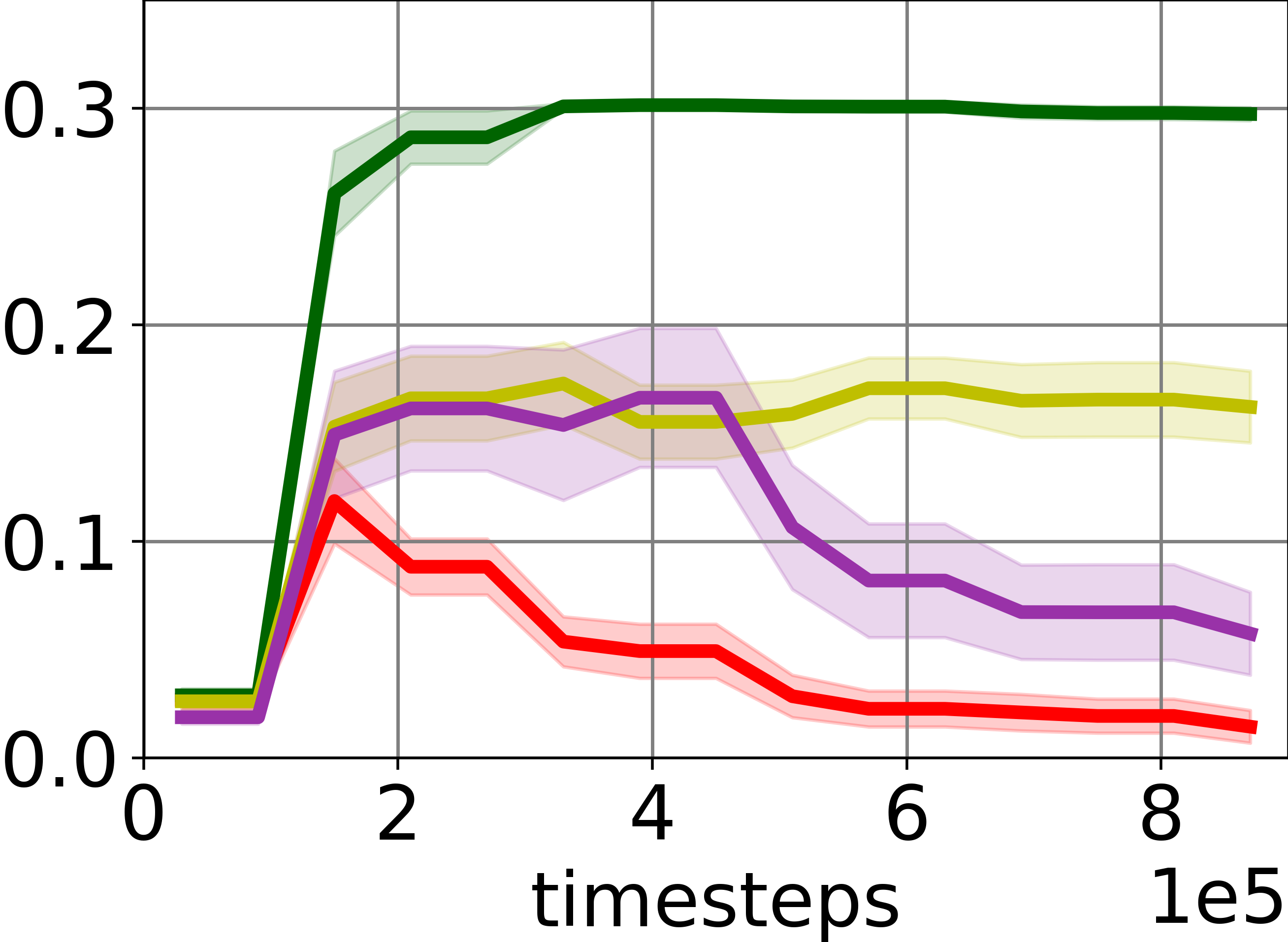
(d) Unsafe rate - 3D task

(e)

Figure 4: The IoU index (higher is better) and unsafe rate (lower is better) of learned constraint function. The two figures on the left are for the 2D reaching task, while the two on the right are for the 3D reaching task. The x-axis indicates the training process, the number of timesteps the agent takes in the environment. Our method outperforms other baseline methods in both environments.

IV-B Results of Different Constraint Learning Methods

The IoU index and the unsafe rate in the two tasks are presented in Fig. 4. All the results are the average of 10 independent runs, and the shaded area represents the variance. Each group of 10 runs uses the same demonstrations and hyper-parameters, but differ in the initialization parameters for the networks.

The proposed method PUCL exhibits superior performance compared to the baseline across both environments and metrics. It achieves a nearly zero unsafe rate at the convergence of the training in both environments. MECL suffers from performance decrease in the late training stage of the 2D task, this is partly caused by the constraint forgetting problem [15]. GPUCL adopts a similar framework to PUCL but performs worse than PUCL, possibly due to the difficulty of fitting a good expert distribution with a very limited numbers of demonstrations.

Despite the superiority of PUCL, one may question why the IoU metric of PUCL is still below 0.8 (2D task) or 0.6 (3D task), relatively far from 1. This is due to the fundamental difficulty of learning the nonlinear constraint without knowing the true parameterization of the constraint and with a limited number of demonstrations. There would be regions in the state space whose feasibility cannot be inferred and decided from the given demonstrations, thus restricting the learning accuracy.

To provide readers with an intuitive understanding, we include visualizations of the 2D constraint learned with PUCL and MECL in Fig. 3. Comparing the learned constraints (red region) with the true constraints (white ellipses) confirms the effectiveness of our method in acquiring a model of a nonlinear constraint. Although the learned constraint area is partially incorrect due to limited demonstrations, it effectively captures the essence of the true constraint and is sufficient for training a safe policy. The baseline method MECL learns a constraint that is more inaccurate, and even some states visited by the demonstrations are classified as infeasible.

IV-C Results of Different Policy Representation and Learning Methods

As introduced in section III-D, we considered two policy representing and learning approaches, namely CRL (Constrained Reinforcement Learning) and DSM (Dynamical System Modulation). We test the two variants in the 3D task and summarize the metrics at convergence and training time of CRL-PUCL and DSM-PUCL in Table II. Here, the recall rate is computed as (True infeasible)/(True infeasible + False feasible), and precision is (True infeasible)/(True infeasible + False infeasible). Training was conducted on a PC with a 12th Intel i9-12900K × 24 and an NVIDIA GeForce RTX 3070. All results are the average of 15 independent runs.

DSM-PUCL and CRL-PUCL achieve similar classification performance in IoU, recall rate and precision, and DSM-PUCL generally exhibits lower variance. For the learned policy, while both methods have an unsafe rate below $1\%$, the rate of DSM-PUCL is much lower than CRL-PUCL. This is because DSM-PUCL modulates the policy in a principled way and features a safety guarantee [25]. DSM-PUCL also requires less training time than CRL-PUCL. Based on these comparison, we conclude that both methods are effective for learning constraints. For robotic tasks where the control variable is the velocity/acceleration of each state dimension, DSM may be more favourable than CRL in terms of training time and policy performance, while CRL is more suitable for more general task with more complex environment dynamics and rewards.

TABLE II: Comparison of two policy representing and learning methods

Methods	CRL-PUCL	DSM-PUCL
IoU	$0.46\pm 0.09$	$0.42\pm 0.01$
Recall rate	$(94.2\pm 4.5)$%	$(99.9\pm 0.1)$ %
Precision	$(47.6\pm 10.0)$%	$(42.1\pm 1.3$) %
Unsafe rate	$(0.47\pm 0.82)$%	$(0.15\pm 0.56)$%
Training time (min)	$13.4\pm 1.7$	$4.7\pm 0.4$

IV-D Constraint Transfer to Variant of the Same Task

One remarkable advantage of learning constraint is that the learned constraint can be transferred to similar task with the same constraint but potentially different goals and rewards. To demonstrate this, we consider the 3D tasks of robot avoiding four tall cylinders forming a convex shape (see Fig. 1). We first applied DSM-PUCL to learn this constraint from 19 demonstrated trajectories (Fig. 1 shows some of the demonstrations.) Then the learned constraint network is transferred to a relevant task with a shifted goal state $s_{g}^{\prime}$ and a set of different starting points. The new nominal policy heading to $s_{g}^{\prime}$ is directly modulated with the transferred constraint, still following DSM in section III-D. This modulated policy, referred to as the transferred policy, is illustrated in Fig. 1, where it also avoids these cups despite the change of goal states. It is worth noting that the transferred constraint can also be utilized by other policy learning/optimization methods such as constrained RL. We adopted DSM in this section only due to its straightforward and rapid modulation process.

V Conclusions and Limitations

This paper proposed the Positive-Unlabeled Constraint Learning method to infer an arbitrary (potentially nonlinear) constraint function from demonstration. The proposed method treats the demonstration as positive data and the higher-reward-winning policy as unlabeled data. It first identifies the reliable infeasible data, and trains a feasibility classifier as constraint function. The benefits of the proposed method were demonstrated learn a 2D or 3D position constraint, using either a constrained RL policy or a DSM policy. It managed to recover and transfer a continuous nonlinear constraint and outperformed other baseline methods in terms of accuracy and safety.

Although PUCL is effective, it only learns a decent but still inaccurate constraint given limited demonstrations and true constraint might be violated in some cases. In the future, we will explore integrating active learning technique to further refine the learned constraint model.

References

- [1] J. Garcıa and F. Fernández, “A comprehensive survey on safe reinforcement learning,” Journal of Machine Learning Research, vol. 16, no. 1, pp. 1437–1480, 2015.
- [2] R. Noothigattu, D. Bouneffouf, N. Mattei, R. Chandra, P. Madan, K. R. Varshney, M. Campbell, M. Singh, and F. Rossi, “Teaching ai agents ethical values using reinforcement learning and policy orchestration,” IBM Journal of Research and Development, vol. 63, no. 4/5, pp. 2–1, 2019.
- [3] G. Chou, D. Berenson, and N. Ozay, “Learning constraints from demonstrations,” in Algorithmic Foundations of Robotics XIII: Proceedings of the 13th Workshop on the Algorithmic Foundations of Robotics 13. Springer, 2020, pp. 228–245.
- [4] D. R. Scobee and S. S. Sastry, “Maximum likelihood constraint inference for inverse reinforcement learning,” in International Conference on Learning Representations, 2020.
- [5] A. Glazier, A. Loreggia, N. Mattei, T. Rahgooy, F. Rossi, and B. Venable, “Learning behavioral soft constraints from demonstrations,” arXiv preprint arXiv:2202.10407, 2022.
- [6] D. L. McPherson, K. C. Stocking, and S. S. Sastry, “Maximum likelihood constraint inference from stochastic demonstrations,” in 2021 IEEE Conference on Control Technology and Applications (CCTA). IEEE, 2021, pp. 1208–1213.
- [7] K. C. Stocking, D. L. McPherson, R. P. Matthew, and C. J. Tomlin, “Maximum likelihood constraint inference on continuous state spaces,” in 2022 International Conference on Robotics and Automation (ICRA). IEEE, 2022, pp. 8598–8604.
- [8] S. Malik, U. Anwar, A. Aghasi, and A. Ahmed, “Inverse constrained reinforcement learning,” in International Conference on Machine Learning. PMLR, 2021, pp. 7390–7399.
- [9] G. Liu, Y. Luo, A. Gaurav, K. Rezaee, and P. Poupart, “Benchmarking constraint inference in inverse reinforcement learning,” International Conference on Learning Representations, 2023.
- [10] J. Jang, M. Song, and D. Park, “Inverse constraint learning and generalization by transferable reward decomposition,” arXiv preprint arXiv:2306.12357, 2023.
- [11] G. Chou, N. Ozay, and D. Berenson, “Learning constraints from locally-optimal demonstrations under cost function uncertainty,” IEEE Robotics and Automation Letters, vol. 5, no. 2, pp. 3682–3690, 2020.
- [12] G. Chou, H. Wang, and D. Berenson, “Gaussian process constraint learning for scalable chance-constrained motion planning from demonstrations,” IEEE Robotics and Automation Letters, vol. 7, no. 2, pp. 3827–3834, 2022.
- [13] G. Chou, N. Ozay, and D. Berenson, “Learning parametric constraints in high dimensions from demonstrations,” in Conference on Robot Learning. PMLR, 2020, pp. 1211–1230.
- [14] J. Bekker and J. Davis, “Learning from positive and unlabeled data: A survey,” Machine Learning, vol. 109, pp. 719–760, 2020.
- [15] B. Peng and A. Billard, “Learning general continuous constraint from demonstrations via positive-unlabeled learning,” 2024. [Online]. Available: https://arxiv.org/abs/2407.16485
- [16] R. S. Sutton and A. G. Barto, Reinforcement learning: An introduction. MIT press, 2018.
- [17] E. Altman, Constrained Markov decision processes. CRC press, 1999, vol. 7.
- [18] B. Zhang and W. Zuo, “Reliable negative extracting based on knn for learning from positive and unlabeled examples.” J. Comput., vol. 4, no. 1, pp. 94–101, 2009.
- [19] L. Liu and T. Peng, “Clustering-based method for positive and unlabeled text categorization enhanced by improved tfidf.” J. Inf. Sci. Eng., vol. 30, no. 5, pp. 1463–1481, 2014.
- [20] A. Stooke, J. Achiam, and P. Abbeel, “Responsive safety in reinforcement learning by pid lagrangian methods,” in International Conference on Machine Learning. PMLR, 2020, pp. 9133–9143.
- [21] B. Peng, J. Duan, J. Chen, S. E. Li, G. Xie, C. Zhang, Y. Guan, Y. Mu, and E. Sun, “Model-based chance-constrained reinforcement learning via separated proportional-integral lagrangian,” IEEE Transactions on Neural Networks and Learning Systems, vol. 35, no. 1, pp. 466–478, 2022.
- [22] B. Peng, Y. Mu, J. Duan, Y. Guan, S. E. Li, and J. Chen, “Separated proportional-integral lagrangian for chance constrained reinforcement learning,” in 2021 IEEE Intelligent Vehicles Symposium (IV). IEEE, 2021, pp. 193–199.
- [23] J. Schulman, F. Wolski, P. Dhariwal, A. Radford, and O. Klimov, “Proximal policy optimization algorithms,” arXiv preprint arXiv:1707.06347, 2017.
- [24] J. Rey, K. Kronander, F. Farshidian, J. Buchli, and A. Billard, “Learning motions from demonstrations and rewards with time-invariant dynamical systems based policies,” Autonomous Robots, vol. 42, pp. 45–64, 2018.
- [25] L. Huber, A. Billard, and J.-J. Slotine, “Avoidance of convex and concave obstacles with convergence ensured through contraction,” IEEE Robotics and Automation Letters, vol. 4, no. 2, pp. 1462–1469, 2019.