A conservative, implicit solver for 0D-2V multi-species nonlinear Fokker-Planck collision equations

Abstract

In this study, we present an optimal implicit algorithm designed to accurately solve the multi-species nonlinear 0D-2V axisymmetric Fokker-Planck-Rosenbluth (FRP) collision equation while preserving mass, momentum, and energy. We rely on the nonlinear Shkarofsky’s formula of FRP (FRPS) collision operator in terms of Legendre polynomial expansions. The key to our meshfree approach is the adoption of the Legendre polynomial expansion for the angular direction and King function (Eq. (54)) expansion for the velocity axis direction. The Legendre polynomial expansion will converge exponentially and the King method, a moment convergence algorithm, could ensure the conservation with high precision in discrete form. Additionally, a post-step projection to manifolds is employed to exactly enforce symmetries of the collision operators. Through solving several typical problems across various nonequilibrium configurations, we demonstrate the superior performance and high accuracy of our algorithm.

I Introduction

In plasma physics, the Fokker-Planck collision operator, known as the Fokker-Planck-Rosenbluth Rosenbluth et al. (1957); Taitano et al. (2015a); Shkarofsky (1963); Shkarofsky et al. (1967) (FRP) or equivalently the Fokker–Planck–Landau Landau (1937) (FPL) operator, is a fundamental tool for describing Coulomb collisions between particles under the assumptions of binary, grazing-angle collisions. This operator is particularly useful for modeling various plasma systems, including those found in laboratory settings such as magnetic confinement fusion (MCF) and inertial confinement fusion (ICF), as well as in natural environments like Earth’s magnetosphere and astrophysical phenomena like solar coronal plasmas. When coupled with Vlasov’s equation Vlasov (1968) and Maxwell’s equations, it provides a comprehensive description of weakly coupled plasma across all collisionality regimes.

The FRP collision operator ensures strict conservation of mass, momentum and energy, while also adhering to the well-established H-theoremBoltzmann (1872) , which guarantees that the entropy of the plasma system increases monotonically with time unless the system reaches a thermal equilibrium state. Throughout history, various formulations of the Fokker-Planck collision operator have been developed to suit different computational and theoretical needs. The FPL collision operator employs a direct integral formulation, making it ideal for conservative algorithms and the H-theorem Boltzmann (1872) due to its symmetric nature. Conversely, the standard FRP collision operator Rosenbluth et al. (1957) represents integral relationships using Rosenbluth potentials, which satisfy the Poisson equation in velocity space. The divergence form of the FRP (FRPD) Chang and Cooper (1970); Taitano et al. (2015a, 2016) collision operator is widely favored in numerical simulations due to its efficiency in fast solvers. Additionally, when employing spherical harmonic expansions, Shkarofsky’s formula of the FRP collision operator (FRPS) Shkarofsky (1963); Shkarofsky et al. (1967) collision operator is often preferred for its computational advantages. These various formulations offer flexibility and efficiency in solving Vlasov-Fokker-Planck (VFP) equations, catering to different computational and theoretical requirements.

Historically, numerous efforts have been dedicated to addressing the numerical solution of the Fokker-Planck collision equation. ThomasThomas et al. (2012) and BellBell et al. (2006) reviewed the different numerical models of Fokker-Planck collision operator for ICF plasma. Cartesian tensor expansionsJohnston (1960); Shkarofsky (1997); Kingham and Bell (2004); Thomas et al. (2009) (CTE) and spherical harmonic expansionsBell et al. (2006); Robinson et al. (2008); Tzoufras et al. (2011, 2013); Wu et al. (2013); Mijin et al. (2020) (SPE) (Legendre polynomial expansionsKrook and Wu (1977); Bell et al. (1981); Matte and Virmont (1982); Shkarofsky et al. (1992); Alouani-Bibi et al. (2004); Zhao et al. (2018) when axisymmetric) are employed to deal with the Fokker-Planck collision operator, which are equivalent to each otherJohnston (1960) .

SPEBell et al. (2006, 1981); Matte and Virmont (1982); Shkarofsky et al. (1992); Alouani-Bibi et al. (2004); Tzoufras et al. (2011) is an important method for moderate nonequilibrium plasma when the ratio of average velocity to thermal velocity is not large. As highlighted by BellBell et al. (2006) , the amplitude of each harmonics will decay exponentially at a rate proportional to ${l(l+1)/2}$. Even in cases of weak collisions, this $l(l+1)/2$ leads to strong damping of higher-order spherical harmonics, naturally terminating the expansion. Early studies by Bell Bell et al. (1981) and Matte Matte and Virmont (1982) focused on including the first two order harmonics to investigate non-Spitzer heat flow in ICF plasmas. Subsequent work by Shkarofsky Shkarofsky et al. (1992) and Alouani-Bibi Alouani-Bibi et al. (2004) extended this approach to higher orders, resulting in the widely used semi-anisotropic collision operator Alouani-Bibi et al. (2004) . In recent years, several VFP codes Bell et al. (2006); Tzoufras et al. (2011); Wu et al. (2011) based on the semi-anisotropic model have been developed. However, effectively calculating the full nonlinear collision operator in the SPE approach remains a challenge Bell et al. (2006); Tzoufras et al. (2011) , particularly in scenarios with large mass disparities such as electron-deuterium collisions in fusion plasmas. While previous simulations based on SPE have adopted the semi-anisotropic model and satisfied mass and energy conservation, achieving momentum conservation exactly in discrete simulations remains difficult.

Other approaches, meshfree methodsPareschi et al. (2000); Filbet and Pareschi (2002); Pataki and Greengard (2011); Askari and Adibi (2015) and finite volume methodMorton K. W. and Mayyers David (2005) (FVM) are also employed to solve the Fokker-Planck collision equation. Fast spectral method based on FFTPareschi et al. (2000); Filbet and Pareschi (2002); Pataki and Greengard (2011) or Hermite polynomial expansionLi et al. (2021) for the FPL collision operator shows the fast convergence of spectral expansion strategyPress et al. (2007) . AskariAskari and Adibi (2015) utilized a meshfree method based on multi-quadric radial basis functions (RBFs) to approximate the solution of the 0D1V Fokker-Planck collision equation. By directly discretize the collision equation with FVM, TaitanoTaitano et al. (2015a, b, 2016, 2017); Daniel et al. (2020) carries out a series of systematic studies based on the 0D-2V FRPD collision operator. They Taitano et al. (2015a) utilized a second-order BDF2 implicit solver and employed the multigrid (MG) methodSaad (2003) in Jacobian-Free Newton-Krylov (JFNK)Saad (2003) solver to overcome the Courant-Friedrichs-Lewy (CFL)Courant et al. (1986) condition. Additionally, by normalizing the velocity space to the local thermal velocities of all species separatelyLarroche (2003) , works in Ref. Taitano et al. (2016) developed a discrete conservation strategy that employs the nonlinear constraints to enforce the continuum symmetries of the collision operator. However, those approaches do not take advantages of the Coulomb collision, similar to SPEBell et al. (2006) , to reduce the number of meshgrids when there is no distinguishing asymmetries in the velocity space.

The challenge of employing SPE Bell et al. (2006) and meshfreeAskari and Adibi (2015) approaches lies in embedding discrete conservation laws within the numerical scheme. According to manifold theory E. et al. (2006) , maintaining a small local error through post-step projection to manifolds preserves the same convergence rate. Therefore, backward error analysisMoore and Reich (2003); Reich (1999) has become a crucial tool for understanding the long-term behavior of numerical integration methods and preserving conservation properties in the numerical scheme.

In this study, our objective is to address the full nonlinearity, discrete conservation laws, and the temporal stiffness challenge of the 0D-2V axisymmetric multi-species FRPS collision equation within the SPE approach. Similar to previous works in Ref. Taitano et al. (2016) , we normalize the velocity spaces to the local thermal velocities for all species separately. However, instead of employing multigrid (MG) technology utilized in Ref. Taitano et al. (2015a) , we employ a King function expansion method (detial in Sec. III.2.1) to overcome the classical CFL condition. To tackle the nonlinear, stiff FRPS collision equations, we propose an implicit meshfree algorithm based on Legendre polynomial expansion for the angular direction, the King method for the velocity axis direction, and the trapezoidal method Press et al. (2007); Rackauckas and Nie (2017) for time integration. Romberg integration Bauer (1961) is employed to compute the kinetic moments with high precision, and backward error analysis Hairer (1999); Reich (1999); Moore and Reich (2003) is applied to ensure numerical conservation of mass, momentum, and energy. The H-theorem Boltzmann (1872) will be satisfied in the discretization process and used as a criterion for the convergence of our meshfree algorithm.

The rest of this paper is organized as follows. Sec.II introduces the FRPS collision equation and its normalization. Discretization of the nonlinear FRPS collision equation is given in Sec.III, include the angular discretization and the King method for the velocity axis dimension. An implicit time discretization and conservation strategies is discussed in Sec.IV. The numerical performance of our meshfree solver, both the accuracy and efficiency, is demonstrated with various multi-species tests in Sec.V. Finally, we conclude our work in Sec.VI.

II The Fokker-Planck-Rosenbluth collision equation

Coulomb collision relaxation in a spatially homogeneous multi-species plasma can be described by the FRP collision equation for the velocity distribution functions of species $a$, $f(\boldsymbol{v},t)$, in velocity space $\boldsymbol{v}$:

$$\frac{\partial}{\partial t}f = \mathfrak{C}\left(\boldsymbol{v},t\right)\leavevmode\nobreak\ .$$ (1)

The term of the right-hand side is total FRP collision operator of species $a$, reads:

$$\mathfrak{C}\left(\boldsymbol{v},t\right) = \sum{{}_{b=1}^{N_{s}}}\mathfrak{C}_{ab}\leavevmode\nobreak\ .$$ (2)

Here, $N_{s}$ is the number of the total number of plasma species and $\mathfrak{C}_{ab}$ is the Shkarofsky’sShkarofsky (1963); Shkarofsky et al. (1967) form of Fokker-Planck-Rosenbluth (FRPS) collision operator for species $a$ colliding with species $b$, reads:

$$\mathfrak{C}_{ab}\left(\boldsymbol{v},t\right)=\Gamma_{ab}\left[4\pi m_{M}Ff+\left(1-m_{M}\right)\nabla_{\boldsymbol{v}}H\cdot\nabla_{\boldsymbol{v}}f+\frac{1}{2}\nabla_{\boldsymbol{v}}\nabla_{\boldsymbol{v}}G:\nabla_{\boldsymbol{v}}\nabla_{\boldsymbol{v}}f\right]\leavevmode\nobreak\ .$$ (3)

In this equation, $\Gamma_{ab}=4\pi\left(\frac{q_{a}q_{b}}{4\pi\varepsilon_{0}m_{a}}\right)^{2}\ln{\Lambda_{ab}}$, $m_{M}=m_{a}/m_{b}$, $m_{a}$ and $m_{b}$ are the masses of species $a$ and $b$, respectively, $q_{a}$ and $q_{b}$ are the charges of species $a$ and $b$, parameters $\varepsilon_{0}$ and $\ln{\Lambda_{ab}}$ are the permittivity constant of vacuum and the Coulomb logarithmHuba (2011) of species $a$ and $b$ which is a weak function of the number of particles in the Debye sphere, the identity $\overleftrightarrow{A}\mathbf{x}:\overleftrightarrow{B}\mathbf{y}=(\mathbf{x}\cdot\overleftrightarrow{B})(\overleftrightarrow{A}\cdot\mathbf{y})$ where $\overleftrightarrow{A}$ is a tensor. Function $F=F(\boldsymbol{v}_{b},t)$ is the distribution function of background species $b$. Functions $H$ and $G$ are Rosenbluth potentials, which are integral operators for the background distribution function $F$, reads:

$$H(\boldsymbol{v}) = \int\frac{1}{\left|\boldsymbol{v}-\boldsymbol{v}_{b}\right|}F\left(\boldsymbol{v}_{b},t\right)\mathrm{d}\boldsymbol{v}_{b},$$ (4)

$$G(\boldsymbol{v}) = \int\left|\boldsymbol{v}-\boldsymbol{v}_{b}\right|F\left(\boldsymbol{v}_{b},t\right)\mathrm{d}\boldsymbol{v}_{b}\leavevmode\nobreak\ .$$ (5)

II.1 Conservation

The FRPS collision operator (give in Eq. (3)) preserves mass, momentum and energy which stem from the its symmetriesBraginskii (1965) . With the inner product definition $\left<f,g\right>_{\boldsymbol{v}}=\int g(\boldsymbol{v})f(\boldsymbol{v})\mathrm{d}\boldsymbol{v}$, the conservation laws can be expressed as follows:

$$\left<1,\mathfrak{C}_{ab}\right>_{\boldsymbol{v}} = \left<1,\mathfrak{C}_{ba}\right>_{\boldsymbol{v}}\quad\equiv\quad 0,$$ (6)

$$m_{a}\left<\boldsymbol{v},\mathfrak{C}_{ab}\right>_{\boldsymbol{v}} = -m_{b}\left<\boldsymbol{v},\mathfrak{C}_{ba}\right>_{\boldsymbol{v}},$$ (7)

$$m_{a}\left<\frac{\boldsymbol{v}^{2}}{2},\mathfrak{C}_{ab}\right>_{\boldsymbol{v}} = -m_{b}\left<\frac{\boldsymbol{v}^{2}}{2},\mathfrak{C}_{ba}\right>_{\boldsymbol{v}}\leavevmode\nobreak\ .$$ (8)

In theory, the FRPS collision operator satisfies the well-known H-theorem. By defining the Boltzmann’s entropy of species $a$, $s_{a}(t)=-\left<f,\ln{f}\right>_{\boldsymbol{v}}$, the total entropy of the plasma system can be expressed as $s_{s}(t)=\sum_{a}s_{a}$. The H-theorem indicates that the total entropy of the isolated plasma system will monotonically increase with the time, unless the total entropy rate of change is zero which means all $f_{a}$ are Maxwellian with a common temperature and average velocity.

II.2 Normalization

In fusion plasmas, additional challenges arise due to disparate thermal velocities, which is a corollary of the immense mass discrepancy ($i$-$e$ collisions) or energy difference ($D$-$\alpha$ collisions). The discrepancy in thermal velocities, illustrated in Fig. 1, amplifies the complexity of discretizing the velocity axis, particularly when mapping the background species distribution function to the collision species domain. Normalizing the distribution function by its local thermal velocity, denoted as $v_{ath}$, has been shown in previous studies Larroche (2003); Taitano et al. (2016) to mitigate these challenges. This normalization not only alleviates the need for different grid meshing requirements between multiple species but also ensures that the thermal velocities evolve consistently over time with the temperature of the distribution functions.

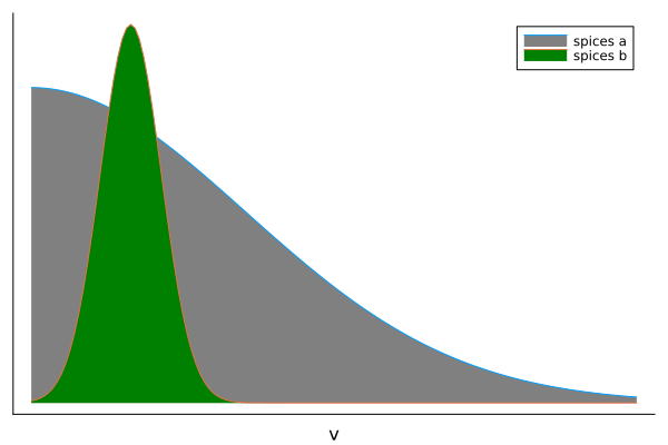
Figure 1: Illustration of the velocity distribution functions for disparate thermal velocities.

We normalize the velocity-space quantities with the local thermal velocity $v_{ath}$ for species $a$:

$$\hat{\boldsymbol{v}}=\boldsymbol{v}/v_{ath}\leavevmode\nobreak\ .$$ (9)

Moreover, the mass, time, charge, thermal velocity, number density $n_{a}$, temperature $T_{a}$ and permittivity are normalized by the proton mass $m_{p}$, characteristic time $\tau_{0}$, elementary charge $e$, vacuum speed of light $c_{0}$, reference number density $n_{20}=10^{-20}\mathrm{m}^{-3}$, practical unit $T_{k}=\mathrm{keV}$ and permittivity of vacuum $\varepsilon_{0}$ respectively. The corresponding dimensionless forms of other quantities are given according to the relationship between them and the above quantities. Thus $\nabla_{\hat{\boldsymbol{v}}}=v_{ath}\nabla_{\boldsymbol{v}}$ and the distribution function could be normalized as the following form:

$$\hat{f}\left(\hat{\boldsymbol{v}},t\right) = n_{a}^{-1}v_{ath}^{3}f\left(\boldsymbol{v},t\right)\leavevmode\nobreak\ .$$ (10)

Hence, the normalized backgroud distribution function and normalized Rosenbluth potentials can be written as:

$$\hat{F}\left(\hat{\boldsymbol{v}}_{b},t\right) = n_{b}^{-1}v_{bth}^{3}F\left(\boldsymbol{v}_{b},t\right)$$ (11)

and

$$\hat{H}(\hat{\boldsymbol{v}}_{ab}) = \frac{v_{bth}}{n_{b}}H(\boldsymbol{v})\ =\ \int\frac{1}{\hat{\boldsymbol{v}}_{ab}-\hat{\boldsymbol{v}}_{b}}\hat{F}\left(\hat{\boldsymbol{v}}_{b},t\right)\mathrm{d}\hat{\boldsymbol{v}}_{b},$$ (12)

$$\hat{G}(\hat{\boldsymbol{v}}_{ab}) = \frac{1}{n_{b}v_{bth}}G(\boldsymbol{v})\ =\ \int\left(\hat{\boldsymbol{v}}_{ab}-\hat{\boldsymbol{v}}_{b}\right)\hat{F}\left(\hat{\boldsymbol{v}}_{b},t\right)\mathrm{d}\hat{\boldsymbol{v}}_{b},$$ (13)

where $\hat{\boldsymbol{v}}_{b}=\boldsymbol{v}_{b}/v_{bth}$ and $\hat{\boldsymbol{v}}_{ab}=\boldsymbol{v}/v_{bth}$. Therefore, the normalized FRPS collision operator (give in Eq. (2)) of species $a$ can be expressed as:

$$\hat{\mathfrak{C}}\left(\hat{\boldsymbol{v}},t\right) = n_{a}^{-1}v_{ath}^{3}\mathfrak{C}=\sum{{}_{b=1}^{N_{s}}}\frac{n_{b}}{v_{bth}^{3}}\hat{\Gamma}_{ab}\hat{\mathfrak{C}}_{ab}$$ (14)

where

$$\hat{\Gamma}_{ab}\left(t\right) = C_{\Gamma}\times 4\pi\left(\frac{Z_{a}Z_{b}}{4\pi m_{a}}\right)^{2}\ln{\Lambda_{ab}},$$ (15)

$$\hat{\mathfrak{C}}_{ab}\left(\hat{\boldsymbol{v}},t\right) = C_{\hat{F}}\hat{F}(\hat{\boldsymbol{v}}_{ab},t)\hat{f}+C_{\hat{H}}\nabla_{\hat{\boldsymbol{v}}_{ab}}\hat{H}\cdot\nabla_{\hat{\boldsymbol{v}}}\hat{f}+C_{\hat{G}}\nabla_{\hat{\boldsymbol{v}}_{ab}}\nabla_{\hat{\boldsymbol{v}}_{ab}}\hat{G}:\nabla_{\hat{\boldsymbol{v}}}\nabla_{\hat{\boldsymbol{v}}}\hat{f}\leavevmode\nobreak\ .$$ (16)

Here, $\nabla_{\hat{\boldsymbol{v}}}$ and $\nabla_{\hat{\boldsymbol{v}}_{ab}}$ are gradients in normalized velocity space $\hat{\boldsymbol{v}}$ and $\hat{\boldsymbol{v}}_{ab}$ respectively, $Z_{a}$ and $Z_{b}$ are the ionization state of species $a$ and $b$, the constant coefficient $C_{\Gamma}={\tau_{0}\omega_{p_{0}}^{4}}/{(n_{20}c_{0}^{3})}$ where $\omega_{p_{0}}=\sqrt{n_{20}e^{2}/(m_{p}\varepsilon_{0})}$. The coefficients in Eq. (16) are:

$$C_{\hat{F}}=4\pi m_{M},\quad C_{\hat{H}}=\left(1-m_{M}\right)v_{bth}/v_{ath},\quad C_{\hat{G}}=\left(v_{bth}/v_{ath}\right)^{2}/2\leavevmode\nobreak\ .$$ (17)

The normalized like-particle collision operator can be obtained from Eq. (16) by replacing $\hat{F}$ and $\hat{\boldsymbol{v}}_{ab}$ by $\hat{f}$ and $\hat{\boldsymbol{v}}$ respectively, reads:

$$\hat{\mathfrak{C}}_{aa}\left(\hat{\boldsymbol{v}},t\right)=4\pi\hat{f}\hat{f}+\frac{1}{2}\nabla_{\hat{\boldsymbol{v}}}\nabla_{\hat{\boldsymbol{v}}}\hat{G}:\nabla_{\hat{\boldsymbol{v}}}\nabla_{\hat{\boldsymbol{v}}}\hat{f}\leavevmode\nobreak\ .$$ (18)

After applying Eq. (14), the FRPS collision equation (1) can be rewritten as:

$$\frac{\partial}{\partial t}f\left(\hat{\boldsymbol{v}},t\right) = \frac{n_{a}}{v_{ath}^{3}}\hat{\mathfrak{C}}\leavevmode\nobreak\ .$$ (19)

To construct a meshfree algorithm, we assume the distribution function, $f(\hat{\boldsymbol{v}},t)$, is a smooth function in the velocity space. It is reasonable that the Coulomb collision always tends to eliminate the fine structures of the distribution functionBell et al. (2006) .

III Discretization of the nonlinear FRPS collision equation

In this work, we consider a meshfree approach (backgroud grids are required) to discretize the 0D-2V axisymmetric FRPS collision operator. SPEJohnston (1960); Robson and Ness (1986) approach is used to discretize the angular components of the normalized FRPS collision operator (given in Eq. (16)). King function expansion method will be used in the velocity axis direction.

III.1 Angular discretization

We choose the SPEJohnston (1960); Robson and Ness (1986) approach (Legendre polynomial expansionsRosenbluth et al. (1957); Matte and Virmont (1982); Shkarofsky et al. (1992); Sunahara et al. (2003); Alouani-Bibi et al. (2004); Zhao et al. (2018) when the system is axisymmetric) to analytically adapt the velocity-space mesh in angular dimensions. Unlike previous studiesBell et al. (2006); Tzoufras et al. (2013); Joglekar et al. (2018) using the semi-anisotropic model, we will retain the full nonlinearity of the FRPS collision operator for all species.

III.1.1 Legendre polynomial expansions

The normalized distribution function of species $a$ can be described by the real function $\hat{f}(\hat{v},\theta,t)$ when system is axisymmetric, which can be expanded based on Legendre polynomials in normalized velocity space $\hat{\boldsymbol{v}}(\hat{v},\theta)$, reads:

$$\hat{f}\left(\hat{v},\mu,t\right) = \sum_{l=0}^{\infty}\hat{f}_{l}^{0}\left(\hat{v},t\right)\mathrm{P}_{l}^{0}\left(\mu\right)\leavevmode\nobreak\ .$$ (20)

Here, $\hat{v}=|\boldsymbol{v}|/v_{ath}$, $\mu=\cos{\theta}$ and $0\leq\theta<\pi$ when choosing the symmetric axis to be the direction $z$ with base vector $\mathbf{e}_{z}$. Function $\mathrm{P}_{l}^{0}(\mu)$ are the $l^{th}$-order Legendre polynomials. Series in Eq. (20) can be truncated with a maximum order, $l_{M}\in\mathbb{N}$ under a specified condition $max|\hat{f}_{l}^{0}(\hat{v},t)|\leq Atol_{df}$. For species $b$, $l_{M}$ will be replaced by $L_{M}$. The convergence of SPE for drift-Maxwellian distribution is depicted in Fig. 2. As we can see, $L_{M}$ as a function of $\hat{u}$ when $\hat{u}\leq 0.5$. For example, $\hat{u}_{a}\leq 2.2\times 10^{-3}$ and $Atol_{df}=10^{-10}$ leads to $L_{M}\leq 3$.

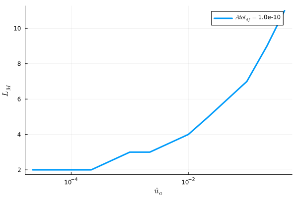
Figure 2: Convergence of SPE for drift-Maxwellian distribution: $L_{M}$ as a function of $\hat{u}_{a}$ when $Atol_{df}=10^{-10}$.

That is owing to the fact that the $l^{th}$-order amplitude will decay exponentially at a rate proportion to $l(l+1)/2$Bell et al. (2006) , which allows a natural termination to the expansions. Hence, function $\hat{f}(\hat{v},\mu,t)$ is represented by a set of amplitudes $\hat{f}_{l}^{0}\left(\hat{v},t\right)$, which are functions of time $t$ and magnitude of normalized velocity $\hat{v}\equiv|\hat{\boldsymbol{v}}|$. The $l^{th}$-order normalized amplitude $\hat{f}_{l}^{0}\left(\hat{v},t\right)$ can be calculated by the inverse transformation of Eq. (20), reads:

$$\hat{f}_{l}^{0}\left(\hat{v},t\right) = \int_{-1}^{1}\hat{f}\left(\hat{v},\mu,t\right)\mathrm{P}_{l}^{0}(\mu)\mathrm{d}\mu\leavevmode\nobreak\ .$$ (21)

Defining Gaussian quadraturePress et al. (2007) :

$$\left<\phi_{n}(x_{i})|y(x_{i})\right>_{G} = \sum_{i=1}^{N_{1}}w_{i}\phi_{n}(x_{i})y(x_{i}),$$ (22)

where the subscript $G$ represents Gaussian, $x_{i}$ and $w_{i}$ are the abscissas and weights of Gaussian quadrature with orthogonal basis function $\phi_{n}(x)$, $N_{1}$ is the number of roots of $\phi_{n}(x)$. Then Eq. (21) can be expressed as:

$$\hat{f}_{l}^{0}\left(\hat{v},t\right)=\sum_{\beta=1}^{l_{M_{1}}}w_{{\mu}_{\beta}}\mathrm{P}_{l}^{0}({\mu}_{\beta})\hat{f}\left(\hat{v},{\mu}_{\beta},t\right)+\mathscr{O}(Atol_{df}),\quad l=0,1,2,\cdots,l_{M}\leavevmode\nobreak\ ,$$ (23)

where

$$l_{M_{1}} = l_{M}+1\leavevmode\nobreak\ .$$ (24)

Gauss-Legendre abscissas will serve as the background mesh grids on the polar angle direction $\mu$. The node ${\mu}_{\beta}$ represents the $\beta^{th}$ one of the total $l_{M_{1}}$ roots of the Legendre polynomial $\mathrm{P}_{l}^{0}(\mu)$, while the associated weight $w_{{\mu}_{\beta}}$ can be computed using the algorithm proposed by Fornberg Fornberg (1998) .

III.1.2 Rosenbluth potentials

Similarly, Rosenbluth potentials of species $a$ due to background species $b$ can be expanded as:

$$\hat{H}\left(\hat{v}_{ab},\mu,t\right) = 4\pi\sum_{L=0}^{\infty}\hat{H}_{L}^{0}\left(\hat{v}_{ab},t\right)\mathrm{P}_{L}^{0}\left(\mu\right),$$ (25)

$$\hat{G}\left(\hat{v}_{ab},\mu,t\right) = 4\pi\sum_{L=0}^{\infty}\hat{G}_{L}^{0}\left(\hat{v}_{ab},t\right)\mathrm{P}_{L}^{0}\left(\mu\right)\leavevmode\nobreak\ .$$ (26)

Here, $\hat{v}_{ab}=|\boldsymbol{v}|/v_{bth}$. The $L^{th}$-order amplitudes of $\hat{H}$ and $\hat{G}$ can be computed in the following integral form:

$$\hat{H}_{L}^{0}\left(\hat{v}_{ab},t\right) = \frac{1}{2L+1}\frac{1}{\hat{v}_{ab}}\left(I_{L,L}^{0}+J_{L+1,L}^{0}\right),$$ (27)

$$\hat{G}_{L}^{0}\left(\hat{v}_{ab},t\right) = \frac{1}{2L+1}\frac{1}{\hat{v}_{ab}}\left(\frac{I_{L+2,L}^{0}+J_{L+1,L}^{0}}{2L+3}-\frac{I_{L,L}^{0}+J_{L-1,L}^{0}}{2L-1}\right)\leavevmode\nobreak\ .$$ (28)

Functions $I_{j,L}^{0}$ and $J_{j,L}^{0}$ are integrals of the normalized background distribution function $\hat{F}_{L}^{0}\left(\hat{v}_{b},t\right)$, similar to Shkarofsky et. al.Shkarofsky et al. (1967); Shkarofsky (1997) , reads:

$$I_{j,L}^{0}\left(\hat{v}_{ab},t\right) = I_{j}\left(\hat{F}_{L}^{0}\right)\ =\ \frac{1}{(\hat{v}_{ab})^{j}}\int_{0}^{\hat{v}_{ab}}(\hat{v}_{b})^{j+2}\hat{F}_{L}^{0}\left(\hat{v}_{b},t\right)\mathrm{d}\hat{v}_{b},$$ (29)

$$J_{j,L}^{0}\left(\hat{v}_{ab},t\right) = J_{j}\left(\hat{F}_{L}^{0}\right)\ =\ (\hat{v}_{ab})^{j}\int_{\hat{v}_{ab}}^{\infty}\frac{\hat{v}_{b}^{2}}{(\hat{v}_{b})^{j}}\hat{F}_{L}^{0}\left(\hat{v}_{b},t\right)\mathrm{d}\hat{v}_{b}\leavevmode\nobreak\ .$$ (30)

The normalized distribution function of the background species $b$, similar to equation (20), can be expressed as:

$$\hat{F}_{L}^{0}\left(\hat{v}_{b},t\right)=\sum_{\beta=1}^{L_{M_{1}}}w_{{\mu}_{\beta}}\mathrm{P}_{L}^{0}({\mu}_{\beta})\hat{F}\left(\hat{v}_{b},{\mu}_{\beta},t\right)+\mathscr{O}(Atol_{df})\leavevmode\nobreak\ .$$ (31)

Here, $L_{M_{1}}=L_{M}+1$.

The partial derivatives of the amplitude of normalized Rosenbluth potential functions with respect to the direction of velocity axis in axisymmetric velocity space are:

$$\frac{\partial}{\partial\hat{v}_{ab}}\hat{H}_{L}^{0}\left(\hat{v}_{ab},t\right) = \frac{1}{2L+1}\frac{1}{\hat{v}_{ab}^{2}}\left[-(L+1)I_{L,L}^{0}+(L)J_{L+1,L}^{0}\right]$$ (32)

and

$$\frac{\partial}{\partial\hat{v}_{ab}}\hat{G}_{L}^{0}\left(\hat{v}_{ab},t\right) = \frac{(L-1)I_{L,L}^{0}-(L)J_{L-1,L}^{0}}{(2L-1)(2L+1)}-\frac{(L+1)I_{L+2,L}^{0}-(L+2)J_{L+1,L}^{0}}{(2L+1)(2L+3)}\leavevmode\nobreak\ .$$ (33)

Similarly, the partial derivative of $\hat{G}_{L}^{0}$ with respect to $\hat{v}_{ab}$ is:

$$\frac{\partial^{2}}{\partial{\hat{\mathscr{v}}}^{2}}\hat{G}_{L}^{0}\left(\hat{v}_{ab},t\right) = {C_{G}^{n2}}_{L}\left(I_{L,L}^{0}+J_{L-1,L}^{0}\right)+{C_{G}^{p2}}_{L}\left(I_{L+2,L}^{0}+J_{L+1,L}^{0}\right)\leavevmode\nobreak\ .$$ (34)

Here, the coefficients ${C_{G}^{n2}}_{L}$ and ${C_{G}^{p2}}_{L}$ are

$${C_{G}^{n2}}_{L} = -\frac{L(L-1)}{(2L-1)(2L+1)},$$ (35)

$${C_{G}^{p2}}_{L} = \frac{(L+1)(L+2)}{(2L+1)(2L+3)}\leavevmode\nobreak\ .$$ (36)

III.1.3 Weak form of FRPS collision equation

Similar to $\hat{f}(\hat{\boldsymbol{v}}$) (give in Eq. (20)), the normalized FRPS collision operator (give in Eq. (14)) can be expanded based on the Legendre polynomials as:

$$\hat{\mathfrak{C}}\left(\hat{\boldsymbol{v}},t\right) = \sum_{l=0}^{\infty}{\hat{\mathfrak{C}}{{}_{l}^{0}}}\left(\hat{v},t\right)\mathrm{P}_{l}^{0}\left(\mu\right)\leavevmode\nobreak\ .$$ (37)

where the $l^{th}$-order amplitude of the normalized multi-species nonlinear FRPS operator is:

$${\hat{\mathfrak{C}}{{}_{l}^{0}}}\left(\hat{v},t\right) = \sum_{b=1}^{N_{s}}\frac{n_{b}}{v_{bth}^{3}}\hat{\Gamma}_{ab}{\hat{\mathfrak{C}}{{}_{l}^{0}}}_{ab}\leavevmode\nobreak\ .$$ (38)

Function ${\hat{\mathfrak{C}}{{}_{l}^{0}}}_{ab}$ is the $l^{th}$-order amplitude of normalized FRPS collision operator for species $a$ colliding with species $b$, which can be expressed as:

$${\hat{\mathfrak{C}}{{}_{l}^{0}}}_{ab}\left(\hat{v},t\right)=\sum_{\beta=1}^{l_{M_{1}}}w_{{\mu}_{\beta}}\mathrm{P}_{l}^{0}({\mu}_{\beta})\hat{\mathfrak{C}}_{ab}\left(\hat{v},{\mu}_{\beta},t\right)+\mathscr{O}(l_{M})\leavevmode\nobreak\ .$$ (39)

The truncation error $\mathscr{O}(l_{M})$ is a small quantity which is a function of $l_{M}$.

Substituting Eq. (20) and (37) into Eq. (19), one can obtain:

$$\frac{\partial}{\partial t}f_{l}^{0}\left(\hat{v},t\right) = \frac{n_{a}}{v_{ath}^{3}}{\hat{\mathfrak{C}}{{}_{l}^{0}}}\leavevmode\nobreak\ .$$ (40)

Multiply both sides of equation (40) by $4\pi m_{a}v^{j+2}\mathrm{d}v$ and integrate over the semi-infinite interval $v=\left[0,\infty\right)$ yields the $(j,l)^{th}$-order FRPS collision equation in weak form, reads:

$$\frac{\partial}{\partial t}\left[4\pi m_{a}n_{a}(v_{ath})^{j}\int_{0}^{\infty}(\hat{v})^{j+2}\hat{f}_{l}^{0}(\hat{v},t)\mathrm{d}\hat{v}\right] = 4\pi m_{a}n_{a}(v_{ath})^{j}\int_{0}^{\infty}(\hat{v})^{j+2}{\hat{\mathfrak{C}}{{}_{l}^{0}}}(\hat{v},t)\mathrm{d}\hat{v}\leavevmode\nobreak\ .$$ (41)

III.1.4 Moment constraints

Generally, defining the $(j,l)^{th}$-order normalized kinetic moment as:

$${\hat{\mathcal{M}}}{{}_{j,l}^{0}}\left(t\right)\ =\ \hat{\mathcal{M}}_{j}\left(\hat{f}_{l}^{0}\right)\ =\ 4\pi\int_{0}^{\infty}(\hat{v})^{j+2}\hat{f}_{l}^{0}\left(\hat{v},t\right)\mathrm{d}\hat{v}\leavevmode\nobreak\ .$$ (42)

Specially, the first few orders relative to the conserved moments are:

$$\hat{n}_{a}\left(t\right) = \hat{\mathcal{M}}_{0,0}^{0}$$ (43)

and

$$\hat{I}_{a}\left(t\right) = \frac{I_{a}}{m_{a}n_{a}v_{ath}}\ =\ \frac{1}{3}\hat{\mathcal{M}}_{1,1}^{0},$$ (44)

$$\hat{K}_{a}\left(t\right) = \frac{K_{a}}{n_{a}T_{a}}\ =\ \hat{\mathcal{M}}_{2,0}^{0}\leavevmode\nobreak\ .$$ (45)

Theoretically, $\hat{n}_{a}(t)\equiv 1$ which is conserved. Momentum $I_{a}(t)=m_{a}n_{a}\boldsymbol{u}_{a}\cdot\mathbf{e}_{z}$ where average velocity $\boldsymbol{u}_{a}(t)=n_{a}^{-1}\int\boldsymbol{v}f\left(\boldsymbol{v},t\right)\mathrm{d}\boldsymbol{v}$, total energy $K_{a}(t)=\frac{m_{a}}{2}\int\boldsymbol{v}^{2}f\left(\boldsymbol{v},t\right)\mathrm{d}\boldsymbol{v}$ and temperature $T_{a}(t)=m_{a}v_{ath}^{2}/2$. The normalized average velocity, $\hat{u}_{a}(t)=\boldsymbol{u}_{a}\cdot\mathbf{e}_{z}/v_{ath}$, which is equivalent to $\hat{I}_{a}$.

Similar to Eq. (42), we give the following definition:

$${\hat{\mathcal{R}}}{{}_{j,l}^{0}}\left(t\right)\ =\ \hat{\mathcal{R}}_{j}\left({\hat{\mathfrak{C}}{{}_{l}^{0}}}\right)\ =\ 4\pi\int_{0}^{\infty}(\hat{v})^{j+2}{\hat{\mathfrak{C}}{{}_{l}^{0}}}\left(\hat{v},t\right)\mathrm{d}\hat{v}\leavevmode\nobreak\ .$$ (46)

Especially, the first few orders of ${\hat{\mathcal{R}}}{{}_{j,l}^{0}}$ related to the conserved qualities can be expressed as:

$$\delta_{t}\hat{n}_{a}\left(t\right) = \frac{\partial_{t}n_{a}}{n_{a}}\ =\ \hat{\mathcal{R}}_{0,0}^{0},$$ (47)

$$\delta_{t}\hat{I}_{a}\left(t\right) = \frac{\partial_{t}I_{a}}{m_{a}n_{a}v_{ath}}\ =\ \frac{1}{3}\hat{\mathcal{R}}_{1,1}^{0},$$ (48)

$$\delta_{t}\hat{K}_{a}\left(t\right) = \frac{\partial_{t}K_{a}}{n_{a}T_{a}}\ =\ \frac{3}{2}\hat{\mathcal{R}}_{2,0}^{0}\leavevmode\nobreak\ .$$ (49)

Applying Eqs. (47)-(49), one can find out the following relation:

$$\delta_{t}\hat{T}_{a}\left(t\right) = \delta_{t}\hat{K}_{a}\left[2\hat{I}_{a}\left(\delta_{t}\hat{I}_{a}-\hat{I}_{a}\frac{1}{v_{ath}}\frac{\mathrm{\partial}v_{ath}}{\mathrm{\partial}t}\right)+\hat{K}_{a}\frac{1}{v_{ath}}\frac{\mathrm{\partial}v_{ath}}{\mathrm{\partial}t}\right]\ \equiv\ 0\leavevmode\nobreak\ .$$ (50)

The above equation can be used as a convergence criterion of our meshfree algorithm for FRPS collision equation (41).

Mass, momentum and energy conservation (6)-(8) in theory based on ${\hat{\mathfrak{C}}{{}_{l}^{0}}}$ can be rewritten as:

$$\left<1,{\hat{\mathfrak{C}}{{}_{0}^{0}}}_{ab}\right>_{\hat{v}} = \left<1,{\hat{\mathfrak{C}}{{}_{0}^{0}}}_{ba}\right>_{\hat{v}_{b}}\quad=\quad 0,$$ (51)

$$m_{a}n_{a}v_{ath}\left<\hat{v},{\hat{\mathfrak{C}}{{}_{1}^{0}}}_{ab}\right>_{\hat{v}} = -m_{b}n_{b}v_{bth}\left<\hat{v}_{b},{\hat{\mathfrak{C}}{{}_{1}^{0}}}_{ba}\right>_{\hat{v}_{b}},$$ (52)

$$\frac{m_{a}n_{a}v_{ath}^{2}}{2}\left<\hat{v}^{2},{\hat{\mathfrak{C}}{{}_{0}^{0}}}_{ab}\right>_{\hat{v}} = -\frac{m_{b}n_{b}v_{bth}^{2}}{2}\left<\hat{v}_{b}^{2},{\hat{\mathfrak{C}}{{}_{0}^{0}}}_{ba}\right>_{\hat{v}_{b}},$$ (53)

where $\left<\hat{v}^{j},g\right>_{\hat{v}}$ denotes the integral of $4\pi(\hat{v})^{j+2}\cdot g$ with respect to $\hat{v}$. These conservation constraints are activated when enforcing discrete conservation (details provided in Sec. IV.1) of the normalized FRPS collision operator  (give in Eq. (16)). Otherwise, they serve as indicators to evaluate the performance of our meshfree algorithm.

III.2 Velocity axis direction

Under the assumption that the function, $f(v,\mu)$ is a smooth function in the velocity space, all the amplitudes, $\hat{f}_{l}^{0}(\hat{v})$ are continuously differentiable. We also assume that the evolution of the system over time is continuous. In contrast to previous work based on the multi-quadric radial basis function Askari and Adibi (2015) , a new function named King (detial in Appendix A) will be used in the velocity axis direction to develop a meshfree algorithm.

III.2.1 King function expansion method

Defining the King function, which is related to the first class of modified Bessel functions, as:

$$\mathcal{K}_{l}\left(v;\iota,\sigma\right)=\frac{(l+1/2)}{\sigma^{2}\sqrt{2\left|\iota\right|v}}\left(\frac{\left|\iota\right|}{\iota}\right)^{l}\mathrm{e}^{-\sigma^{-2}\left(v^{2}+\iota^{2}\right)}\mathrm{Besseli}\left(\frac{2l+1}{2},2\frac{\left|\iota\right|}{\sigma^{2}}v\right)\leavevmode\nobreak\ .$$ (54)

Here, the independent variable $v\in[0,\mathbb{R}^{+}]$ and the parameter $l\in\mathbb{N}$ which is the order of the King function, parameters $\iota$ and $\sigma$ are the characteristic parameters of the King function which satisfy $\sigma\in\mathbb{R}^{+}$ and $\iota\in\mathbb{R}$ respectively. When two groups of characteristic parameters $\left(\iota_{1},\sigma_{1}\right)$ and $\left(\iota_{2},\sigma_{2}\right)$, with weights $\hat{n}_{a_{1}}$ and $\hat{n}_{a_{2}}$ satisfy

$$\left|\frac{\sigma_{1}}{\sigma_{2}}-1\right|+\left|\frac{\iota_{1}}{\iota_{2}}-1\right| \leq rtol,$$ (55)

where $rtol$ is a given relative tolerance with a default value $rtol=10^{-10}$ in this paper, we call $\mathcal{K}_{l}\left(v;\iota_{1},\sigma_{1}\right)$ and $\mathcal{K}_{l}\left(v;\iota_{2},\sigma_{2}\right)$ are identical, $\mathcal{K}_{l}\left(v;\iota_{0},\sigma_{0}\right)$ with weight $\hat{n}_{a_{0}}=\hat{n}_{a_{1}}+\hat{n}_{a_{2}}$. Eq. (55) is the indistinguishable condition for the King function.

The $l^{th}$-order King function, $\mathcal{K}_{l}\left(\hat{v};\hat{u}_{a},\hat{v}_{ath}\right)$ (give in Eq. (54)) has the same asymptotic behaviour (detial in Appendix A) as the $l^{th}$-order amplitude of the normalized distribution function, $\hat{f}_{l}^{0}(\hat{v},t)$ (give in Eq. (23)). Hence, we can effectively approximate $\hat{f}_{l}^{0}(\hat{v},t)$ based on the King function, reads:

$$\hat{f}_{l}^{0}\left(\hat{v},t\right) = C_{3}\sum{{}_{s=1}^{N_{K}}}\left[\hat{n}_{a_{s}}\mathcal{K}_{l}\left(\hat{v};\hat{u}_{a_{s}},\hat{v}_{{ath}_{s}}\right)\right]\leavevmode\nobreak\ .$$ (56)

Similar for the $l^{th}$-order amplitude of the normalized distribution function of the background species $b$, $\hat{F}_{L}^{0}\left(\hat{v}_{b},t\right)$. Here, the constant coefficient $C_{3}=\sqrt{2\pi}/{\pi^{3/2}}$, $N_{K}\in\mathbb{N}^{+}$ is the number of the components, which is a given number at the first step and will be decided by L01jd2NK scheme later (Sec. in III.2.2).

The King method (56) is a moment convergence algorithm (demonstrated in Sec. V.1). In this paper we assume that parameters $\hat{n}_{a_{s}}$, $\hat{u}_{a_{s}}$ and $\hat{v}_{{ath}_{s}}$ are independent on $l$, which means that normalized function $\hat{f}\left(\hat{v},\mu,t\right)$ can be approximated by $N_{K}$ Gaussian functions, reads $\hat{f}\left(\hat{v},\mu,t\right)=\sum_{s=1}^{N_{K}}\frac{1}{\pi^{3/2}}\frac{\hat{n}_{a_{s}}}{\hat{v}_{{ath}_{s}}^{3}}\mathrm{e}^{-\left(\hat{\boldsymbol{v}}-\hat{u}_{a_{s}}\mathbf{e}_{z}\right)^{2}}.$ This is reasonable and efficient especially when every sub-component $\mathcal{K}_{l}$ is not far from thermal equilibrium state, $|\hat{u}_{a_{s}}|\ll 1$.

Multiplying both sides of equation (56) by $4\pi\hat{v}^{j+2}\mathrm{d}\hat{v}$ and integrating over the semi-infinite interval $\hat{v}=\left[0,\infty\right)$ yields:

$${\mathcal{M}}{{}_{j,l}^{0}}\left(t\right)\ =\ \left\{\begin{aligned} &{C_{M}}_{j}^{l}\sum_{s=1}^{N_{K}}\hat{n}_{a_{s}}(\hat{v}_{{ath}_{s}})^{j}\left[1+\sum_{k=1}^{j/2}C_{j,l}^{k}\left(\frac{\hat{u}_{a_{s}}}{\hat{v}_{{ath}_{s}}}\right)^{2k}\right],\quad l\in 2\mathbb{N},\\ &{C_{M}}_{j}^{l}\sum_{s=1}^{N_{K}}\hat{n}_{a_{s}}(\hat{v}_{{ath}_{s}})^{j}\left(\frac{\hat{u}_{a_{s}}}{\hat{v}_{{ath}_{s}}}\right)^{l}\left[1+\sum_{k=1}^{(j-1)/2}C_{j,l}^{k}\left(\frac{\hat{u}_{a_{s}}}{\hat{v}_{{ath}_{s}}}\right)^{2k}\right],\quad l\in 2\mathbb{N}+1\leavevmode\nobreak\ .\\ \end{aligned}\right.$$ (57)

Regard above equations as characteristic parameter equations. Here, coefficients $C_{j,l}^{k}$ and ${C_{M}}_{j}^{l}$ are:

$$C_{j,l}^{k} = 2^{k}\frac{(2l+1)!!C_{(j-l)/2}^{k}}{(2l+2k+1)!!}$$ (58)

and

$${C_{M}}_{j}^{l} = \frac{1}{2^{(j-l)/2}}\frac{(l+j+1)!!}{(2l-1)!!}\leavevmode\nobreak\ .$$ (59)

Especially, when all $\hat{u}_{a_{s}}$ are zeros, the characteristic parameter equations will be:

$${\hat{\mathcal{M}}}{{}_{j,l}^{0}}(t) = {C_{M}}_{j}^{l}\sum_{s=1}^{N_{K}}\hat{n}_{a_{s}}(\hat{v}_{{ath}_{s}})^{j},\quad l\in 2\mathbb{N}\leavevmode\nobreak\ .$$ (60)

Note that ${\hat{\mathcal{M}}}{{}_{j,l}^{0}}$ represents the normalized kinetic moment (give in Eq. (42)) computed from the amplitude of distribution function before being smoothed by King method. Parameters $\hat{n}_{a_{s}}$, $\hat{u}_{a_{s}}$ and $\hat{v}_{{ath}_{s}}$ can be calculated by solving any $3N_{K}$ different orders $(j,l)$ characteristic parameter constraint equations  (57). To solve the characteristic parameter constraint equations, the following section provides two specific algorithms which are convergent for higher-order moments.

III.2.2 L01jd2NK scheme for parameters $\hat{n}_{a_{s}}$, $\hat{u}_{a_{s}}$ and $\hat{v}_{{ath}_{s}}$

Generally, any $3N_{K}$ normalized kinetic moments, ${\hat{\mathcal{M}}}{{}_{j,l}^{0}}$ could be used in Eq. (57) to determine parameters $\hat{n}_{a_{s}}$, $\hat{u}_{a_{s}}$ and $\hat{v}_{{ath}_{s}}$. Due to the rapid damping of the higher-order harmonics, the first few harmonics in the expression (20) contain much of the most important physics for many plasma physical problems of interest. Hence, with the assumption that parameters $\hat{n}_{a_{s}}$, $\hat{u}_{a_{s}}$ and $\hat{v}_{{ath}_{s}}$ are independent on $l$, we propose the following scheme by choosing the kinetic moments of the first two amplitudes of normalized distribution function with

$$(j,l)\in\left\{(2j_{p}+l,l)|j_{p}\in\mathbb{N},0\leq l\leq 1,0\leq 2j_{p}+l<3N_{K}\right\}\leavevmode\nobreak\ .$$ (61)

which will be regarded as the L01jd2nh scheme. Especially, when $(j,l)=(1,1)$, Eq. (57) gives:

$$\sum_{s=1}^{N_{K}}\hat{n}_{a_{s}}\hat{u}_{a_{s}} = {\hat{\mathcal{M}}}{{}_{1,1}^{0}}/3\ =\ \hat{u}_{a}\leavevmode\nobreak\ .$$ (62)

When $(j,l)=(0,0)$ and $(j,l)=(2,0)$, Eq. (57) gives:

$$\sum{{}_{s=1}^{N_{K}}}\hat{n}_{a_{s}} = {\hat{\mathcal{M}}}{{}_{0,0}^{0}}\ =\ \hat{n}_{a},$$ (63)

$$\sum{{}_{s=1}^{N_{K}}}\hat{n}_{a_{s}}\left(\frac{3}{2}\hat{v}_{{ath}_{s}}^{2}+\hat{u}_{a_{s}}^{2}\right) = \hat{\mathcal{M}}_{2,0}^{0}\ =\ \frac{3}{2}+\left(\hat{u}_{a}\right)^{2}\leavevmode\nobreak\ .$$ (64)

This implies that when $N_{K}\geq 1$, the L01jd2nh (similar to L01jd2) scheme can ensure mass, momentum and energy convergence during the optimization process.

After computing the normalized kinetic moments ${\hat{\mathcal{M}}}{{}_{j,l}^{0}}$ from Eq. (72), parameters $\hat{n}_{a_{s}}$, $\hat{u}_{a_{s}}$ and $\hat{v}_{{ath}_{s}}$ can be solved from Eq. (57) by using a least squares methodFong and Saunders (2011) (LSM), named Levenberg-MarquardtWright and Holt (1985); Kanzow et al. (2004) method. To enclose the nonlinear FRPS collision equation (41), high-order amplitudes of normalized distribution function when $l\geq 2$ can be approximated by Eq. (56). Then, the first two derivatives of $\hat{f}_{l}^{0}(\hat{v},t)$ with respect to $\hat{v}$ can be given analytically based on Eq. (56). The number of King function at the $(k+1)^{th}$ time step will be:

$$N_{K}(t_{k+1}) = N_{K}(t_{k})-dN_{K}(t_{k})$$ (65)

where

$$dN_{K}(t_{k})=\begin{aligned} \left\{\begin{array}[]{cc}0,&Eq.\leavevmode\nobreak\ (\ref{Dvhths})==false,\\ 1,&Eq.\leavevmode\nobreak\ (\ref{Dvhths})==true\leavevmode\nobreak\ .\end{array}\right.\end{aligned}$$ (66)

When parameters $\hat{n}_{a_{s}}$ of species $a$ are all nearly to be constants, a more effective scheme named as L01jd2, instead of L01jd2nh, can be used. Here, by assuming $\hat{n}_{a_{s}}$ are constants and any $2N_{K}$ normalized kinetic moments, ${\hat{\mathcal{M}}}{{}_{j,l}^{0}}$ could be used in Eq. (57) to give parameters $\hat{u}_{a_{s}}$ and $\hat{v}_{{ath}_{s}}$. In L01jd2 scheme,

$$(j,l)\in\left\{(2j_{p}-l,l)|j_{p}\in\mathbb{N}^{+},0\leq l\leq 1,1\leq j_{p}<N_{K}\right\}\leavevmode\nobreak\ .$$ (67)

L01jd2NK scheme is given by integrating L01jd2nh scheme and L01jd2 scheme with the following criterion,

$$\delta\hat{n}_{a_{s}}\ =\ \left|\hat{n}_{a_{s}}(t_{k+1})-\hat{n}_{a_{s}}(t_{k})\right|/\hat{n}_{a_{s}}(t_{k})\leavevmode\nobreak\ .$$ (68)

When parameters $\hat{n}_{a_{s}}$ of species $a$ satisfy $\delta\hat{n}_{a_{s}}\ \leq\ rtol_{nhC},s=1,2,\cdots,N_{K}$ where $rtol_{nhC}$ is a given relative tolerance, L01jd2 scheme will be performed. Or else, L01jd2nh scheme will be performed in L01jd2NK scheme. In this paper, parameter $rtol_{nhC}=0.1$ unless otherwise stated.

Especially, when parameters $\hat{u}_{a_{s}}$ are all zeros, the L01jd2nh scheme reduces to:

$$(j,l)\in\left\{(2j_{p}-2,l)|j_{p}\in\mathbb{N}^{+},1\leq j_{p}\leq 2N_{K},l=0\right\},$$ (69)

and L01jd2 scheme will be:

$$(j,l)\in\left\{(2j_{p},l)|j_{p}\in\mathbb{N}^{+},1\leq j_{p}\leq N_{K},l=0\right\}\leavevmode\nobreak\ .$$ (70)

In theory when $\hat{u}_{a_{s}}$ are all zeros, enforcing Eqs. (62)-(64) gives:

$$\hat{\mathcal{M}}_{1,1}^{0}=0,\quad{\hat{\mathcal{M}}}{{}_{0,0}^{0}}\ =\ \frac{2}{3}\hat{\mathcal{M}}_{2,0}^{0}=1\leavevmode\nobreak\ .$$ (71)

Eq. (69) and Eq. (70) show that if $N_{K}$ increases by one, the convergent order $j$ increases by two in the L01jd2 scheme and by four in the L01jd2nh scheme when $N_{K}\geq 2$.

It is important to note that the L01jd2NK scheme is effective only when the assumption that parameters $\hat{n}_{a_{s}}$, $\hat{u}_{a_{s}}$, and $\hat{v}_{{ath}_{s}}$ are independent of $l$ is satisfied. A self-adaptive scheme based on the general normalized kinetic moments ${\hat{\mathcal{M}}}{{}_{j,l}^{0}}$, which is effective for the general situation when parameters $\hat{n}_{a_{s}}$, $\hat{u}_{a_{s}}$, and $\hat{v}_{{ath}_{s}}$ are dependent on $l$, will be developed in future studies.

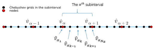
Figure 3: The uniform background nodes and the Chebyshev grids in the subinterval.

III.2.3 Discretization of the velocity axis

To compute the normalized kinetic moments ${\hat{\mathcal{M}}}{{}_{j,l}^{0}}$ (42) in Eq. (57) and the Shkarofsky’s integrals (give in Eqs. (29)-(30)), a set of background meshgrids in velocity axis direction are needed. Applying uniform background nodes $[v_{\alpha}]$ with number $N_{n}=2^{n_{2}}+1$ and normalized velocity axis domain $[0,\hat{v}_{M}]$, the grid spacing is $\mathrm{\Delta}\hat{v}_{\alpha}=\hat{v}_{M}/2^{n_{2}}$ where $n_{2}\in\mathbb{N}^{+}$. The default value of parameters $\hat{v}_{M}$ and $n_{2}$ are $\hat{v}_{M}=10$ and $n_{2}=7$. Hence, the default number of nodes, $N_{n}=129$ unless otherwise stated.

The normalized kinetic moments ${\hat{\mathcal{M}}}{{}_{j,l}^{0}}$ (42) will be calculated by Romberg integralBauer (1961) . For convenience, the value of integration and its relative error can be expressed as:

$${\hat{\mathcal{M}}}{{}_{j,l}^{0}}(t),Error\left({\hat{\mathcal{M}}}{{}_{j,l}^{0}}\right) = \left<(\hat{v}_{\alpha})^{j}|\hat{f}_{l}^{0}(\hat{v}_{\alpha},t)\right>_{R}\leavevmode\nobreak\ .$$ (72)

Here, $\left<(\hat{v})^{j}|\hat{f}_{l}^{0}(\hat{v})\right>_{R}$ denotes Romberg integral of function $(\hat{v})^{j+2}\hat{f}_{l}^{0}(\hat{v})$ and function $Error\left({\hat{\mathcal{M}}}{{}_{j,l}^{0}}\right)$ is estimated upper bound of integral error of ${\hat{\mathcal{M}}}{{}_{j,l}^{0}}$. Similarly, Eq. (46) also will be computed by Romberg integral, reads:

$${\hat{\mathcal{R}}}{{}_{j,l}^{0}}(t),Error\left({\hat{\mathcal{R}}}{{}_{j,l}^{0}}\right) = \left<(\hat{v}_{\alpha})^{j}|{\hat{\mathfrak{C}}{{}_{l}^{0}}}(\hat{v}_{\alpha},t)\right>_{R}\leavevmode\nobreak\ .$$ (73)

The relative errors, $Error\left({\hat{\mathcal{M}}}{{}_{j,l}^{0}}\right)$ and $Error\left({\hat{\mathcal{R}}}{{}_{j,l}^{0}}\right)$ can be used as indicators to evaluate the quality of backgroud meshgrids. These indicators could be used to construct a self-adaptive algorithm which will be developed in the future.

The Shkarofsky’s integrals (given in Eqs. (29)-(30)) involve variable upper/lower bound integration, which can be computed on a set of refined grids. We add $N_{\alpha}-2$ auxiliary grids in the inner interval $[\hat{v}_{\alpha},\hat{v}_{\alpha+1}]$ to create the $\alpha^{th}$ subinterval $[\hat{v}_{{\alpha}k}],k=1,2,\cdots,N_{\alpha}$, as showed in Fig. 3. For the background species $b$, we define $\hat{v}_{ab_{\alpha_{k}}}=(v_{ath}/v_{bth})\hat{v}_{{\alpha}_{k}}$. Hence, the Shkarofsky’s integrals (given in Eqs. (29)-(30)) can be calculated by a parallel Clenshaw-Curtis (CC) quadraturePress et al. (2007), which is a type of Gauss-Chebyshev quadrature. This method reads:

$$I_{j,L}^{0}\left(\hat{v}_{ab_{\alpha}},t\right) = \begin{aligned} \left\{\begin{array}[]{cc}0,&\alpha=1,\\ \frac{1}{(\hat{v}_{ab_{\alpha}})^{j}}\sum_{s=2}^{\alpha}\left<\left(\hat{v}_{ab_{s_{k}}}\right)^{j}|\hat{F}_{L}^{0}(\hat{v}_{ab_{s_{k}}},t)\right>_{CC},&2\leq\alpha\leq 2^{n_{2}}+1,\end{array}\right.\end{aligned}$$ (74)

$$J_{j,L}^{0}\left(\hat{v}_{ab_{\alpha}},t\right) = \begin{aligned} \left\{\begin{array}[]{cc}0,&\alpha=2^{n_{2}}+1,\\ (\hat{v}_{ab_{\alpha}})^{j}\sum_{s=\alpha}^{2^{n_{2}}}\left<\left(\hat{v}_{ab_{s_{k}}}\right)^{-j}|\hat{F}_{L}^{0}(\hat{v}_{ab_{s_{k}}},t)\right>_{CC},&1\leq\alpha\leq 2^{n_{2}}\leavevmode\nobreak\ .\end{array}\right.\end{aligned}$$ (75)

Function $\hat{F}_{L}^{0}\left(\hat{v}_{ab},t\right)$ is the background distribution function on the velocity space of species $a$, which can be obtained easily from the analytic function $\hat{F}_{L}^{0}\left(\hat{v}_{b},t\right)$ (56). Clenshaw-Curtis quadrature can be expressed as:

$$\left<(x_{k})^{j}|g(x_{k})\right>_{CC} = \sum_{k=1}^{N_{\alpha}}w_{k}(x_{k})^{j+2}g(x_{k})\leavevmode\nobreak\ .$$ (76)

The corresponding integral weight $w_{k}$ is calculated according to the algorithm in Ref.Fornberg (1998) .

In this paper, the number of subintervals $N_{\alpha}$ is set to a given constant $N_{0}$. Thus, the total number of background meshgrids in the velocity axis direction is $N_{v}=(N_{0}-1)(N_{n}-2)+N_{0}$ and $N_{v2}=l_{M_{1}}\times N_{v}$ for the total velocity space. Given the default value $N_{0}=7$ unless otherwise stated, we have $N_{v}=769$. It is important to note that $N_{v}$ and $N_{v2}$ are used primarily in the Rosenbluth potentials step (Sec. III.1.2), otherwise the maximum number of background meshgrids in the velocity space is determined by number of nodes, $N_{n}$. It is worth mentioning that the King function serves as a smoothing step in our meshfree algorithm, similar to the MG method in Taitano’s FVM approachTaitano et al. (2015a) . Together with the following implicit scheme in time discretization (Sec. IV), our algorithm overcomes the classical CFL condition limit.

IV Time integration

The weak form of FRPS collision equation (41) in discrete form can be expressed as:

$$\frac{\partial}{\partial t}\left[4\pi m_{a}n_{a}(v_{ath})^{j}\left<(\hat{v}_{\alpha})^{j}|\hat{f}_{l}^{0}(\hat{v}_{\alpha},t)\right>_{R}\right]=4\pi m_{a}n_{a}(v_{ath})^{j}\left<(\hat{v}_{\alpha})^{j}|{\hat{\mathfrak{C}}{{}_{l}^{0}}}(\hat{v}_{\alpha},t)\right>_{R}\leavevmode\nobreak\ .$$ (77)

When integrals (72)-(73) are convergent and accurate, the above equation represents the $(j,l)^{th}$-order kinetic moment evolution equation, which reads:

$$\frac{\partial}{\partial t}\left[m_{a}n_{a}(v_{ath})^{j}{\hat{\mathcal{M}}}{{}_{j,l}^{0}}\right] = m_{a}n_{a}(v_{ath})^{j}{\hat{\mathcal{R}}}{{}_{j,l}^{0}}\leavevmode\nobreak\ .$$ (78)

The first few orders related to conserved moments can be expressed as:

$$\frac{\partial}{\partial t}n_{a} = n_{a}{\hat{\mathcal{R}}}{{}_{0,0}^{0}},$$ (79)

$$\frac{\partial}{\partial t}I_{a} = \frac{1}{3}m_{a}n_{a}v_{ath}{\hat{\mathcal{R}}}{{}_{1,1}^{0}},$$ (80)

$$\frac{\partial}{\partial t}K_{a} = \frac{3}{4}m_{a}n_{a}v_{ath}^{2}\hat{\mathcal{R}}_{2,0}^{0}\leavevmode\nobreak\ .$$ (81)

Thermal velocity, $v_{ath}$ is a function of $m_{a},n_{a},I_{a}$ and $K_{a}$, reads:

$$v_{ath} = \sqrt{\frac{2}{3}\left(\frac{2K_{a}}{m_{a}n_{a}}-\left(\frac{I_{a}}{m_{a}n_{a}}\right)^{2}\right)}\leavevmode\nobreak\ .$$ (82)

The above equations (77), (79)-(82) along with Eqs. (16), (38), (39) and (56)-(72) constitute the final semi-discrete scheme of the nonlinear FRPS collision equations with constraint Eqs. (50)-(53). A standard trapezoidalRackauckas and Nie (2017) scheme, which is a second-order implicit Range-Kutta method, will be used for integration in time. The inner iteration during every timestep will be terminated when $|v_{ath}(t_{k_{i}})/v_{ath}(t_{k_{i-1}})-1|\leq 10^{-6}$, where $v_{ath}(t_{k_{i}})$ is thermal velocity of species $a$ at the $i^{th}$ stage of the $k^{th}$ timestep. The main procedure is given in the following pseudo-code (Algorithm 1), which is implemented in Julia language.

1 From inputs $\left[f_{0}(\boldsymbol{v},t_{0}),f_{1}(\boldsymbol{v},t_{0}),\cdots,f_{s}(\boldsymbol{v},t_{0})\right]$ with total number $N_{K_{0}}$:

2Initial $n_{a}$, $u_{a}$ $v_{ath}$ and $\hat{f}_{l}^{0}(\hat{v}_{\alpha},t_{0})$ (23) with parameter $l_{M_{1}}$ for all species

3Initial ${\hat{\mathcal{M}}}{{}_{0,0}^{0}}$, ${\hat{\mathcal{M}}}{{}_{1,1}^{0}}$ and $\hat{\mathcal{M}}{{}_{2,0}^{0}}$ according to Eq. (72) for all species

4For $a=1,2,\cdots,N_{s}$

5 1 Compute normalized kinetic moments ${\hat{\mathcal{M}}}{{}_{j,l}^{0}}$ (72), except for ${\hat{\mathcal{M}}}{{}_{0,0}^{0}}$, ${\hat{\mathcal{M}}}{{}_{1,1}^{0}}$ and $\hat{\mathcal{M}}{{}_{2,0}^{0}}$

6 2 Solve equations (57) to give parameters $\hat{n}_{a_{s}}$, $\hat{u}_{a_{s}}$, $\hat{v}_{{ath}_{s}}$ and update $\hat{f}_{l}^{0}(\hat{v}_{\alpha},t)$ (56)

7For $b=1,2,\cdots,N_{s}$

8 3 Evaluate $\frac{\partial}{\partial\hat{v}}\hat{f}_{l}^{0}(\hat{v},t)$, $\frac{\partial^{2}}{\partial{\hat{v}}^{2}}\hat{f}_{l}^{0}(\hat{v},t)$ and $\hat{F}_{L}^{0}(\hat{v}v_{ath}/v_{bth},t)$ according to Eq. (56)

9 4 Calculate the Shkarofsky’s integrals (29)-(30) in the scheme (74)-(75)

10 5 Calculate Eqs. (27)-(28) and Eqs. (31)-(34) to give the amplitudes of Rosenbluth potentials and its related derivatives

11 6 Compute the normalized FRPS collision operator $\hat{\mathfrak{C}}_{ab}(\hat{v}_{\alpha},t)$ by solving Eqs. (16)

12 7 Compute the amplitudes of FRPS collision operator ${\hat{\mathfrak{C}}{{}_{l}^{0}}}_{ab}(\hat{v}_{\alpha},t)$ by Eqs. (39)

13 8 Evaluate ${\hat{\mathcal{R}}}{{}_{j,l}^{0}}$ and $Error\left({\hat{\mathcal{R}}}{{}_{j,l}^{0}}\right)$ by computing the Romberg integrals (73)

14 If Conservation enforcing $==$ True

15  9A Update $\frac{\partial}{\partial t}n_{a}$, $\frac{\partial}{\partial t}I_{a}$, $\frac{\partial}{\partial t}K_{a}$ according to conservation enforcing algorithm 2.

16 Else

17  9B Update $\frac{\partial}{\partial t}n_{a}$, $\frac{\partial}{\partial t}I_{a}$, $\frac{\partial}{\partial t}K_{a}$ according to Eqs. (79)-(81)

18 End

19End

20End

2110 Compute $\hat{f}_{l}^{0}(v_{\alpha},t)$ and $n_{a}$, $I_{a}$, $K_{a}$ by solving Eqs. (77), (79)-(81) with trapezoidal method

2211 Update $u_{a}$ (88), $v_{ath}$ (89), ${\hat{\mathcal{M}}}{{}_{0,0}^{0}}$ (90), ${\hat{\mathcal{M}}}{{}_{1,1}^{0}}$ (91) and $\hat{\mathcal{M}}{{}_{2,0}^{0}}$ (92)

12 Update parameters $l_{M_{1}}$ (24), $N_{K}$ (65) at the new timestep

Algorithm 1 Meshfree algorithm for FRPS collision equation with conservation constrains

IV.1 Conservation enforcing

Integrals (47)-(49) will be accurate at least for one species during two-species collision processes (detial in Sec.V.1). Convergence criterion for conservation with high accuracy in two-species collision processes can be expressed as:

$$\mathrm{min}(\delta_{t}\hat{C}_{a},\delta_{t}\hat{C}_{b}) \ll 1,$$ (83)

where

$$\delta_{t}\hat{C_{a}} = \left|Error(\delta_{t}\hat{n}_{a})\right|+\left|Error(\delta_{t}\hat{I_{a}})\right|+\left|Error(\delta_{t}\hat{K}_{a})\right|$$ (84)

and similar for $\delta_{t}\hat{C_{b}}$.

From manifold theoryE. et al. (2006) , post-step projection to manifolds maintains consistent convergence rate, and conservation properties can be preserved if the local solution errors remain sufficiently small. Consequently, adding a conservation strategy into our meshfree algorithm becomes feasible. This strategy enforces discrete conservation equations  (51)-(53) based on the integrals  (47)-(49) of species $b$, which offer more accurate representations during two-species collision processes. This conservation strategy will convergence when criterion (give in Eq. (83)) is satisfied.

According to the conservation constraint Eqs. (52)-(53), rates of momentum and energy change of species $a$ with respect to time at the $k^{th}$ timestep can be expressed as:

$$\frac{\partial}{\partial t}{I_{a}}_{k} = -\frac{\partial}{\partial t}{I_{b}}_{k},$$ (85)

$$\frac{\partial}{\partial t}{K_{a}}_{k} = -\frac{\partial}{\partial t}{K_{b}}_{k}\leavevmode\nobreak\ .$$ (86)

All the rates of density number change will be zeros when enforcing conservation:

$${n_{a}}_{k+1} = {n_{a}}_{k}.$$ (87)

In the implicit method, ${I_{a}}_{k+1}={I_{a}}_{k}+{\Delta}_{t_{k}}\frac{\partial}{\partial t}{I_{a}}_{k+1}^{*}$ and ${K_{a}}_{k+1}={K_{a}}_{k}+{\Delta}_{t_{k}}\frac{\partial}{\partial t}{K_{a}}_{k+1}^{*}$, where $A_{k+1}^{*}$ denotes the value of $A$ at the last iterative stage of $(k+1)^{th}$ step. Consequently, the average velocity and thermal velocity of species $a$ at the $(k+1)^{th}$ timestep are:

$${u_{a}}_{k+1} = \frac{{I_{a}}_{k+1}}{m_{a}{n_{a}}_{k+1}},$$ (88)

$${v_{ath}}_{k+1} = \sqrt{\frac{2}{3}\left[\frac{2{K_{a}}_{k+1}}{m_{a}{n_{a}}_{k+1}}-\left({u_{a}}_{k+1}\right)^{2}\right]}\leavevmode\nobreak\ .$$ (89)

Thus, the normalized average velocity of species $a$ will be ${\hat{u}_{a}}{{}_{k+1}}={u_{a}}_{k+1}/{v_{ath}}_{k+1}$. Applying Eqs. (62)-(64) gives:

$${\hat{\mathcal{M}}}{{}_{0,0}^{0}}(t_{k+1}) \equiv 1,$$ (90)

$${\hat{\mathcal{M}}}{{}_{1,1}^{0}}(t_{k+1}) = 3{\hat{u}_{a}}{{}_{k+1}},$$ (91)

$$\hat{\mathcal{M}}{{}_{2,0}^{0}}(t_{k+1}) = 3/2+\left({\hat{u}_{a}}{{}_{k+1}}\right)^{2}\leavevmode\nobreak\ .$$ (92)

Conservation enforcing algorithm will be given in the following pseudo-code (Algorithm 2).

1 From inputs ${\hat{\mathcal{R}}}{{}_{j,l}^{0}}$ and $Error\left({\hat{\mathcal{R}}}{{}_{j,l}^{0}}\right)$ of species $a$ and species $b$:

2Initial $\frac{\partial}{\partial t}n$, $\frac{\partial}{\partial t}I$, $\frac{\partial}{\partial t}K$ for species $a$ and species $b$, according to Eqs. (79)-(81)

31 Evaluate whether $\mathrm{min}(\delta_{t}\hat{C}_{a},\delta_{t}\hat{C}_{b})\ll 1$ (give in Eq. (83))

4If $\delta_{t}\hat{C}_{a}\geq\delta_{t}\hat{C}_{b}$

5 2A $\frac{\partial}{\partial t}I_{a}=-\frac{\partial}{\partial t}I_{b}$, $\quad\frac{\partial}{\partial t}K_{a}=-\frac{\partial}{\partial t}K_{b}$

6Else

7 2B $\frac{\partial}{\partial t}I_{b}=-\frac{\partial}{\partial t}I_{a}$, $\quad\frac{\partial}{\partial t}K_{b}=-\frac{\partial}{\partial t}K_{a}$

8End

93 $\frac{\partial}{\partial t}n=0$ for all species

104 Output $\frac{\partial}{\partial t}n$, $\frac{\partial}{\partial t}I$, $\frac{\partial}{\partial t}K$ for all species.

Algorithm 2 Algorithm for enforcing conservation during two-species collision processes

Applying the above conservation enforcing scheme, the accuracy of the conservation (51)-(53) will be determined by the precision of the more accurate species, rather than the less precise species. It is worth noting that small local solution errors of $\delta_{t}\hat{n}$, $\delta_{t}\hat{I}$ and $\delta_{t}\hat{K}$ for at least one species during two-species Coulomb collision process are necessary condition for convergence. This condition (give in Eq. (83)) will be checked at every timestep in our meshfree algorithm.

IV.2 Timestep

The Coulomb collision process encompasses multiple dynamical times-scales (such as inter-species time-scale, self-collision time-scale, relaxation time-scale of conserved moments, et al.), and is therefore stiff. In this paper, a timestep of $\Delta t=2^{-5}$ (unless otherwise stated) will be employed for fixed timestep cases. Self-adaptive timestep will be utilized (unless otherwise stated) to improve the algorithm performances, which is given by the following algorithm:

$${\Delta}_{t_{k+1}} = \mathrm{min}\left(ratio_{dt_{k}}\times{\Delta}_{t_{k}},ratio_{M_{j}}\times\left|\frac{\partial_{t}{y_{k}}}{y_{k}}\right|\right).$$ (93)

Here, the subscripts $k$ denote the time level and $y$ represents momentum $I$ and total energy $K$ for all species. $\Delta_{t_{k}}=1$ at the initial timestep. Parameters $ratio_{dt_{k}}$ and $ratio_{M_{j}}$ are given constants, with default values of $ratio_{dt_{k}}=1.1$ and $ratio_{M_{j}}=0.01$ in this paper. For cases utilizing self-adaptive timestep, nearly all timesteps satisfy $10^{-3}\leq\Delta t\leq 0.1$.

As a contrast, the explicit timestep size decided by the CFL conditionTaitano et al. (2015a) is computed as:

$${\Delta}_{t}^{Exp} = R_{CFL}\times\underset{l=0,1,\cdots,l_{M}\atop a,b=1,2,\cdots,N_{s}}{\mathrm{min}}\left\{\frac{\mathrm{\Delta}\hat{v}}{A_{l}^{0}{{}_{ab}}},\frac{(\mathrm{\Delta}\hat{v})^{2}}{D_{l}^{0}{{}_{ab}}}\right\}.$$ (94)

Here, the parameter $R_{CFL}=0.1$ is used in explicit method for long-term stability, $A_{l}^{0}{{}_{ab}}$ and $D_{l}^{0}{{}_{ab}}$ are the transport coefficients in the FRPS collision operator (give in Eq. (3)), defined as:

$$A_{l}^{0}{{}_{ab}} = \frac{n_{a}}{v_{ath}^{3}}\frac{n_{b}}{v_{bth}^{3}}\times C_{\hat{H}}\hat{\Gamma}_{ab}\frac{\partial}{\partial\hat{v}_{ab}}\hat{H}_{L}^{0},$$ (95)

and

$$D_{l}^{0}{{}_{ab}} = \frac{n_{a}}{v_{ath}^{3}}\frac{n_{b}}{v_{bth}^{3}}\times C_{\hat{G}}\hat{\Gamma}_{ab}\frac{\partial^{2}}{\partial{\hat{\mathscr{v}}}^{2}}\hat{G}_{L}^{0}\leavevmode\nobreak\ .$$ (96)

For large mass disparity situation where $\mathrm{min}(m_{M},1/m_{M})\ll 1$, the explicit timestep size will be decided by the first-order effect terms stem from $A_{l}^{0}{{}_{ab}}$, or else decided by the second-order effect terms stem from $D_{l}^{0}{{}_{ab}}$.

V Numerical results

To demonstrate the convergence and effectiveness of our meshfree method for solving the Fokker-Planck collision equation (19), we will assess the performance of our algorithm with various examples of varying degrees of complexity.

In the benchmarks conducted in this session, the initial distribution functions for particles at $t=0$ are drifting Maxwellian distributions with a specified density $n_{a}$, average velocity $u_{a}$ and temperature $T_{a}$, which can be written as:

$$f(\boldsymbol{v},t) = \frac{n_{a}}{v_{ath}^{3}}\hat{f}(\hat{v},\mu,t)\ =\ \frac{1}{\pi^{3/2}}\frac{n_{a}}{(v_{ath})^{3}}\sum_{s=1}^{N_{K_{0}}}\left[\frac{\hat{n}_{a_{s}}}{(\hat{v}_{{ath}_{s}})^{3}}\mathrm{e}^{-\left(\hat{\boldsymbol{v}}-\hat{u}_{a_{s}}\mathbf{e}_{z}\right)^{2}}\right],$$ (97)

For all cases, all the parameters are normalized values with units defined in Sec.II.2. Unless otherwise specified, the number of King functions $N_{K_{0}}=1$ at the initial timestep. Hence, the default values of parameters, $\hat{n}_{a_{s}}=\hat{v}_{{ath}_{s}}=1$ and $\hat{u}_{a_{s}}=\hat{u}_{a}$. For L01jd2 scheme, the number of King function, $N_{K}$ during time evolution will remain equivalent to $N_{K_{0}}$, while a maximum value of $N_{K}$ will be specified in L01jd2NK and L01jd2nh schemes. In this paper, the default solver is L01jd2NK scheme when $max(m_{M},1/m_{M})\sim 1$, and L01jd2 scheme when $max(m_{M},1/m_{M})\gg 1$.

V.1 Two-species thermal equilibration

In this case, we demonstrate the convergence performance of our meshfree algorithm on two-species thermal equilibration, which is a commonly used benchmark to evaluate schemes for solving the Fokker-Planck collision equation. The parameters are $m_{a}=2$, $m_{b}=3$, $Z_{a}=Z_{b}=1$, $n_{a}=n_{b}=1$, $u_{a}=u_{b}=0$, $T_{a}=10$ and $T_{b}=20$ in this case. Theoretically values for the temperature and momentum when the system reaches the equilibrium state can be obtained using the momentum and energy conservation equations:

$${I_{s}}_{k} = \sum_{a}\left(m_{a}{n_{a}}_{k}{u_{a}}_{k}\right)\ \equiv\ \sum_{a}\left(m_{a}{n_{a}}_{0}{u_{a}}_{0}\right),$$ (98)

$${K_{s}}_{k} = \frac{1}{2}\sum_{a}\left[3{n_{a}}_{k}{T_{a}}_{k}+m_{a}{n_{a}}_{k}({u_{a}}_{k})^{2}\right]\ \equiv\ \frac{1}{2}\sum_{a}\left[3n_{a}{T_{a}}_{0}+m_{a}{n_{a}}_{0}({u_{a}}_{0})^{2}\right]\leavevmode\nobreak\ .$$ (99)

The initial total momentum and energy are ${I_{s}}_{0}=0$ and ${K_{s}}_{0}=45$, respectively. From the conservation Eqs. (98)-(99), the finial average velocity and temperatures of the thermal equilibrium state should be $u_{\infty}=0$ and $T_{\infty}=15$, respectively.

The two-species thermal equilibration model, as described given by BraginskiiBraginskii (1958) , provides a semianalytical asymptotic temperature evolution equation can be expressed as:

$$\frac{\partial}{\partial t}T_{a} = \nu_{T}^{ab}\left(T_{a}-T_{b}\right)\leavevmode\nobreak\ .$$ (100)

Here the characteristic collision rate $\nu_{T}^{ab}$ is Huba (2011) :

$$\nu_{T}^{ab} \approx 441.72\times\frac{\sqrt{m_{a}m_{b}}\left(Z_{a}Z_{b}\right)^{2}n_{b}}{\left(m_{a}T_{b}+m_{b}T_{a}\right)^{3/2}}\ln{\Lambda_{ab}}\leavevmode\nobreak\ .$$ (101)

The temperature relaxation time is $\tau_{T}^{ab}=1/\nu_{T}^{ab}$. The characteristic time $\tau_{0}$ will be equivalent to the initial temperature relaxation time unless otherwise specified.

The semianalytical equation (100) is solved by using the standard explicit Runge-KuttaRackauckas and Nie (2017) method of order 4, and the results are plotted in Fig. 4. The temperatures are plotted as functions of time and compared against the numerical solution of our kinetic model with a fixed timestep of $\Delta t=2^{-5}$ and L01jd2NK scheme with the maximum number of King function $N_{K}=2$. Fig. 4 illustrates good agreement between our fully kinetic model and the semianalytical solution. Moreover, upon comparing the results of L01jd2 and L01jd2NK ($N_{K}=2$) with the semianalytical solution, we observe that the temperature decay rate of L01jd2NK is a slightly faster than that of Braginskii’s within the initial time interval ($t<0.58$ in this case), but this trend reverses when $t\geq 0.58$ (Similar to the behavior observed in the FVM’s approach as shown in the Fig.14 of Ref.Taitano et al. (2015a)). However, the results of L01jd2 scheme is strictly adhere to the semianalytical solution, as shown in the lower subplot of Fig. 4.

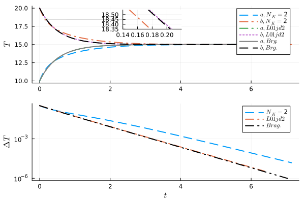
Figure 4: Two-species temperature equilibration with fixed timestep, $\Delta t=2^{-5}$: Temperatures (upper) and their relative disparity of temperatures (lower), $\Delta T=\left|{T_{a}}_{k}-{T_{b}}_{k}\right|/\left({T_{a}}_{k}+{T_{b}}_{k}\right)$ as functions of time. The color lines represent the numerical solution while the gray and black lines represent the Braginskii’s values.

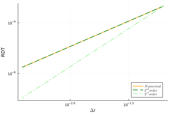
Figure 5: Two-species temperature equilibration with fixed timestep, $\Delta t$: Demonstration of second-order convergence of the time discretization scheme.

Solid lines in Fig. 5 depict the relative deviation of temperature between our kinetic model and an reference values $T_{ref}$, $RDT=\left|T_{kin}-T_{ref}\right|/T_{ref}$ at $t=0.5$ as functions of the fixed timestep, $\Delta t$. The reference value, $T_{ref}$ is computed with a small enough timestep, $\Delta t=2^{-11}$, in our kinetic model. The results indicate that our meshfree algorithm exhibits $2^{nd}$-order convergence in time discretization.

The time histories of the errors in the conserved quantities, namely, discrete number density (or mass), momentum, energy conservation,

$$\Delta n_{s} = (N_{s})^{-1}\sum_{a}\left|{n_{a}}_{k}/{n_{a}}_{0}-1\right|,$$ (102)

$$\Delta I_{s} = \left|{I_{s}}_{k}/{I_{s}}_{0}-1\right|,$$ (103)

$$\Delta K_{s} = \left|{K_{s}}_{k}/{K_{s}}_{0}-1\right|,$$ (104)

and entropy conservation,

$$\Delta s_{s} = \frac{1}{{s_{s}}_{k}}\frac{\partial}{\partial t}{s_{s}}_{k},$$ (105)

are shown in Fig. 6 for varying number of background meshgrids, $(n_{2},N_{0})$.

The discrete mass conservation can be achieved with high precision for all given $(n_{2},N_{0})$ even without enforcing conservation. The discrete momentum conservation and H-theorem are preserved all the time. The discrete error of the energy conservation rapidly decreases with an increase of number of backgroud meshgrids and reaches the level of round-off error when $(n_{2},N_{0})=(8,8)$, corresponding to a total number of nodes $N_{n}=257$. Since $l_{M_{1}}=1$ for two-species temperature equilibration, the total number of background meshgrids is $N_{v2}=l_{M_{1}}\times N_{v}=1793$ for Rosenbluth potentials step III.1.2. The results of $\Delta K_{s}$ in Fig. 6 indicate that the convergence order of the velocity-space discretization scheme is about 16. The convergence orderFornberg (1996) of a discrete algorithm is evaluated using:

$$order = \frac{\log(\epsilon_{n_{2}-1}/\epsilon_{n_{2}})}{\log(2)}\leavevmode\nobreak\ .$$ (106)

Here, we assume that $\epsilon_{n_{2}}=\mathscr{O}[(h_{n_{2}})^{order}]$ where $h_{n_{2}}$ is the grid size when grid number is $2^{n_{2}}$. The number of time steps in this case is $N_{t}=122$, determined by the termination condition $\Delta s_{s}\leq 10^{-10}$.

Figure 6: Two-species temperature equilibration without enforcing conservation: Discrete conservation errors as functions of time and number of background meshgrids, $(n_{2},N_{0})$.

The relative errors of Romberg integrals for the first few orders of $\hat{\mathcal{R}}_{j,l}^{0}$ (46), $\delta_{t}\hat{n}_{a}$ (47), $\delta_{t}\hat{I}_{a}$ (48), $\delta_{t}\hat{K}_{a}$ (49) and convergence criterion $\delta_{t}\hat{T}_{a}$ (50) during two-species Coulomb collisions are plotted in Fig. 7 when $(n_{2},N_{0})=(7,7)$. We can observe that all the relative errors are at the level of round-off error. The maximal errors occur at the initial moment and decay to be the level of round-off error during a collision time scale. Convergence criterion $\delta_{t}\hat{T}_{a}$ is equal to the theoretical value all the time means that our meshfree algorithm can be well convergent.

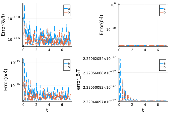
Figure 7: Two-species temperature equilibration without enforcing conservation: Romberg integral errors of $\delta_{t}\hat{n}$, $\delta_{t}\hat{I}$, $\delta_{t}\hat{K}$ and convergence criterion $\delta_{t}\hat{T}$ respect to time $t$ when $(n_{2},N_{0})=(7,7)$.

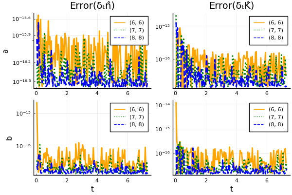
Figure 8: Two-species temperature equilibration without enforcing conservation: Romberg integral errors of $\delta_{t}\hat{n}$ and $\delta_{t}\hat{K}$ respect to time for collision species $a$ and $b$ with various $(n_{2},N_{0})$.

The relation between relative errors and orders $(n_{2},N_{0})$ is shown in Fig. 8. In all cases, the relative errors are all significantly smaller that one, which means that condition (give in Eq. (83)) is satisfied all the time. Particularly, the relative errors of species $a$ are at the level of round-off error all the time. However, the orange solid line representing species $b$ in Fig. 8 shows that both the relative errors of $\delta_{t}\hat{n}_{b}$ and $\delta_{t}\hat{K}_{b}$ are two orders of magnitude larger than the round-off error when $(n_{2},N_{0})=(6,6)$ at the initial moments. This discrepancy can lead to significant discrete errors in energy conservation (see Fig. 6). Furthermore, Fig. 8 also indicates that as the number of grids $(n_{2},N_{0})$ increases, the errors of species $b$ rapidly decrease to the level of round-off error. This suggests that integrals (47)-(49) will be accurate at least for one species during two-species collision process and the integration accuracy of the poor one can be improved by refining the background meshgrids.

Figure 9: Two-species temperature equilibration with enforcing conservation: Discrete conservation errors as functions of time and number of background meshgrids, $(n_{2},N_{0})$.

When applying the conservation enforcing algorithm 2, the time histories of the related conservation errors, $\Delta n_{s}$ and $\Delta K_{s}$ are plotted in Fig. 9 for varying number of background meshgrids, $(n_{2},N_{0})$. As expected, all the discrete conservation can be achieved with a high precision for all given $(n_{2},N_{0})$.

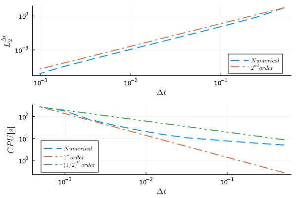
Figure 10: Two-species temperature equilibration with fixed timestep, $\Delta t$: Demonstration of second-order convergence of the time discretization scheme in $L_{2}$-norm (upper) and the CPU time as function of timestep, $\Delta t$.

We can also demonstrate second-order time convergence of the trapezoidal scheme by computing the $L_{2}$-norm of relative difference in solution against a reference solution,

$$L_{2}^{{\Delta}_{t}} = \sqrt{\left<f_{l}^{0}{{}^{\Delta t}}/f_{l}^{0}{{}^{\Delta t_{ref}}}-1,f_{l}^{0}{{}^{\Delta t}}/f_{l}^{0}{{}^{\Delta t_{ref}}}-1\right>}\leavevmode\nobreak\ .$$ (107)

Here, $f_{l}^{0}{{}^{\Delta t_{ref}}}$ is the solution obtained using a reference timestep size, $\Delta t_{ref}=2^{-11}$; refer to Fig. 10 (upper) when $(n_{2},N_{0})=(7,7)$. As expected, second-order convergence is realized with the refinement of ${\Delta}_{t}$. The CPU time as function of $\Delta t$ when $(n_{2},N_{0})=(7,7)$ is also plotted in the lower subplot of Fig. 10. The total solution time scales approximately as $\mathscr{O}(1/\Delta t)$. Compared to the explicit timestep with $\Delta_{t}^{Exp}\approx 1.5\times 10^{-3}$ (estimated by Eq. (94)) in this case, a timestep greater than two order of magnitude can be used in our meshfree algorithm with acceptable precision.

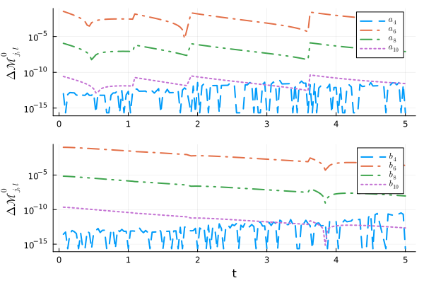
Figure 11: Two-species temperature equilibration without enforcing conservation: Time discretization errors of the non-conserved moments as functions of time with various $j$ when $\Delta t=2^{-5}$, $N_{K}=2$ and $(n_{2},N_{0})=(7,7)$.

Fig. 11 illustrates the time discretization errors of the non-conserved moments, $\Delta{\hat{\mathcal{M}}}{{}_{j,l}^{0}}$ as functions of time with various $j$ when $j\geq 4$, $\Delta t=2^{-5}$, $N_{K}=2$ and $(n_{2},N_{0})=(7,7)$. Here,

$$\Delta{\hat{\mathcal{M}}}{{}_{j,l}^{0}} = \left|M_{j,l}^{0}(t_{k+1})-{\hat{\mathcal{M}}}{{}_{j,l}^{0}}(t_{k+1})\right|/\left|{\hat{\mathcal{M}}}{{}_{j,l}^{0}}(t_{k+1})-M_{j,l}^{0}(t_{k})\right|$$ (108)

which estimates the relative error produced by velocity discretization. By applying Eqs. (62)-(64) in L01jd2NK scheme, the time discretization errors of the conserved moments (give in Eq. (108)) for all species will be exactly zero. Moreover, when $\Delta{\hat{\mathcal{M}}}{{}_{j,l}^{0}}\leq rtol_{NK}$ where $rtol_{NK}$ is a given relative tolerance, we say that the optimization of $(j,l)^{th}$-order normalized kinetic moments is convergent. In this paper, parameter $rtol_{NK}$ is set to $10^{-11}$ unless otherwise stated. As observed in Fig. 11, the moment with order $j=6$ exhibites the maximum deviation when $N_{K}=2$, which is no more than $6.6\%$ for all species in this case. The time discretization errors of the convergent order, $j=4$, are generally no more than $10^{-11}$.

The high-order moment convergence property of the present method is further investigated. Time discretization errors of the non-conserved moments, $\Delta{\hat{\mathcal{M}}}{{}_{j,l}^{0}}$, when $t_{k}\approx 0.47$ as functions of $N_{K}$ with various $j$ are depicted in Fig. 12. A refined timestep and background meshgrids, $\Delta t=2^{-6}$ and $(n_{2},N_{0})=(8,8)$ will be used in this test. As shown in Fig. 12, all the discretization errors of the non-conserved moments, $\Delta{\hat{\mathcal{M}}}{{}_{j,l}^{0}}$, decrease with the increase of $N_{K}$. Moreover, the highest convergent order is $j=2$ when $N_{K}=1$, $j=4$ when $N_{K}=2$ and $j=6$ when $N_{K}=3$. Hence, we demonstrate that King method (Sec. III.2.1) is a moment convergence algorithm.

Figure 12: Two-species temperature equilibration without enforcing conservation: Time discretization errors of the non-conserved moments as functions of $N_{K}$ with various $j$ when $\Delta t=2^{-6}$, $t_{k}\approx 0.47$ and $(n_{2},N_{0})=(8,8)$.

Figure 13: Two-species temperature equilibration with temperatures, $T_{a}=10$, $T_{b}=100$ and fixed timestep, $\Delta t=2^{-5}$ when $N_{K}=2$ and $(n_{2},N_{0})=(9,7)$.

In situations with large thermal velocity disparity where $v_{th_{f}}/v_{th_{s}}\gg 1$, to achieve the same precision without self-adaptive in velocity axis direction requires a refined backgroud meshgrids by increase $n_{2}$. Here, $n_{2}$ is directly proportional to the maximum ratio of thermal velocity, $v_{th_{f}}/v_{th_{s}}$. For example, when $T_{a}=10$, $T_{b}=100$ and the other parameters are the same as above case, the temperatures solved by L01jd2NK scheme with a fixed timestep $\Delta t=2^{-5}$, $N_{K}=2$ and $(n_{2},N_{0})=(9,7)$ are plotted as functions of time in Fig. 13. As expected, the results show good agreement between our fully kinetic model and the semianalytical solution.

V.2 Electron-Deuterium thermal equilibration

To verify the convergence for situations with large mass disparity, we consider $e$-$D$ temperature equilibration with parameters $m_{e}=1/1836$, $m_{D}=2$, $-Z_{e}=Z_{D}=1$, $n_{e}=n_{D}=1$, $\hat{u}_{e}=\hat{u}_{D}=0$, $T_{e}=1$ and $T_{D}=10$ in this case. The final average velocity and temperatures of the thermal equilibrium state should be $u_{\infty}=0$ and $T_{\infty}=5.5$, respectively. This case is solved by the L01jd2 scheme with a self-adaptive timestep and the number of timestep, $N_{t}=792$ when the termination condition is $\Delta s_{s}\leq 10^{-8}$. We will demonstrate that L01jd2 scheme is a good approximation of the fully kinetic mode for the situation with large mass disparity.

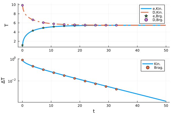
Figure 14: $e$-$D$ thermal equilibration with enforcing conservation when solved by L01jd2 with fixed timestep, $\Delta t=2^{-5}$: Average velocities and temperatures as function of time $t$ when $(n_{2},N_{0})=(7,7)$.

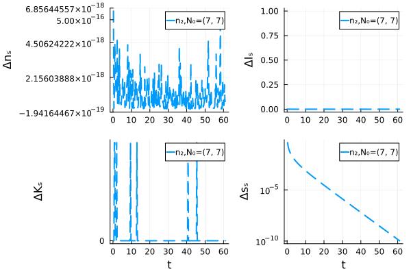
Figure 15: $e$-$D$ thermal equilibration with enforcing conservation when solved by L01jd2 with fixed timestep, $\Delta t=2^{-5}$: Discrete conservation errors as functions of time when $(n_{2},N_{0})=(7,7)$.

Temperatures of species $e$ and $D$ are plotted as function of time $t$ in Fig. 14, which shows that correct equilibrium values are reached. The time histories of the errors in discrete number density, momentum, energy conservation (102)-(104) and entropy conservation are depicted in Fig. 15. The local relative errors, $Error(\delta_{t}\hat{n})$ and $Error(\delta_{t}\hat{K})$ of species $e$ and $D$ are plotted in Fig. 16 when enforcing conservation. As can be seen, all the errors of species $D$ are at the level of round-off errors and errors of $e$ are acceptably small, which conforms to the convergence criterion for conservation (give in Eq. (83)).

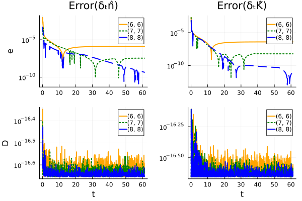
Figure 16: $e$-$D$ thermal equilibration with enforcing conservation when solved by L01jd2 with fixed timestep, $\Delta t=2^{-5}$: Local errors of $\delta_{t}\hat{n}$ and $\delta_{t}\hat{K}$ as functions of time with various $(n_{2},N_{0})$.

To verify the effectiveness of L01jd2 for situations with large mass disparity, we verify its convergence with the following criterion:

$$\Delta_{0}f_{l}^{0}(\hat{v}_{\alpha},t_{k+1}) = \left|f_{l}^{0}{{}^{*}}(\hat{v}_{\alpha},t_{k+1})-f_{l}^{0}(\hat{v}_{\alpha},t_{k+1})\right|/\left|f_{l}^{0}{{}^{*}}(\hat{v}_{\alpha},t_{k+1})-f_{l}^{0}(\hat{v}_{\alpha},t_{k})\right|=C_{0}\leavevmode\nobreak\ .$$ (109)

and

$$\Delta_{2}f_{l}^{0}=\left({N_{v}}\right)^{-1}\sum{{}_{\alpha=1}^{N_{v}}}\delta f_{l}^{0}(\hat{v}_{\alpha},t_{k+1})\leavevmode\nobreak\ .$$ (110)

Here,

$$\delta f_{l}^{0}(\hat{v}_{\alpha},t_{k+1}) = \left|f_{l}^{0}{{}^{*}}(\hat{v}_{\alpha},t_{k+1})-f_{l}^{0}(\hat{v}_{\alpha},t_{k+1})\right|/\left|\Delta t\times f_{l}^{0}{{}^{*}}(\hat{v}_{\alpha},t_{k+1})\right|=C_{2}(\Delta t)^{2}\leavevmode\nobreak\ .$$ (111)

Functions $f_{l}^{0}{{}^{*}}(\hat{v},t_{k+1})$ and $f_{l}^{0}(\hat{v},t_{k+1})$ are the values of the $l^{th}$-order amplitude of distribution function before and after smoothed by the King method at the $(k+1)^{th}$ timestep for species $a$, respectively.

The convergence of function $\Delta_{2}f_{l}^{0}$ is illustrated in Fig. 17, where the finial time is consistently set to $t_{k+1}=0.5$. The right-lower subplot in Fig. 17 provides clear evidence of the convergence of King method with second-order accuracy as $\Delta t$ is refined. With a sufficiently small timestep, such as $\Delta t=0.01$, the maximum relative disparity of the distribution function before and after being smoothed by the King method does not exceed $11\%$ for species $e$ and $10^{-5}$ for species $D$ in this scenario. This can be observed from the distribution function at $k^{th}$ and $(k+1)^{th}$ time steps for species $e$ and $D$ in Fig. 17 (upper). The detail of the relative disparity as function of $\hat{v}$ is plotted in the lower-left subplot of Fig. 17 when $\Delta t=2^{-5}$.

Similarly, the convergence of function $\Delta_{0}f_{l}^{0}$ at the grid point $v_{\alpha}=1.68\times 10^{-2}$ is illustrated in Fig. 18. The lower subplots exhibit that the parameter $C_{0}$ tends to stabilize as a constant with the refinement of $\Delta t$ at single velocity axis node, i.e. $\hat{v}_{\alpha}=0.0338$ for species $e$ and $\hat{v}_{\alpha}=0.0583$ for species $D$. As we can see, for species $D$, which exhibits a higher precision of distribution function, $\Delta_{0}f_{l}^{0}(\hat{v}_{\alpha}=0.0583)$ remains bellows $0.1$ for all provided timesteps and does not exceed $1\%$ when $\Delta t=2^{-5}$. Considering the high precision of conservation in discrete and acceptable timestep $\Delta t=2^{-5}$, the L01jd2 scheme is a good approximation of the full kinetic mode for situation with large mass disparity.

Figure 17: e-D temperature equilibration with enforcing conservation when solved by L01jd2 with fixed timestep, $\Delta t=2^{-5}$: Criterion $C_{2}$ for situation with large mass disparity.

Figure 18: e-D temperature equilibration with enforcing conservation when solved by L01jd2 with fixed timestep, $\Delta t=2^{-5}$: Criterion $C_{0}$ for situation with large mass disparity.

V.3 Electron-Deuterium temperature and momentum equilibration

We consider $e$-$D$ temperature and momentum equilibration with parameters $m_{e}=1/1836$, $m_{D}=2$, $-Z_{e}=Z_{D}=1$, $n_{e}=n_{D}=1$, $\hat{u}_{e}=0.1$, $\hat{u}_{D}=-3.162\times 10^{-2}$, $T_{e}=1$ and $T_{D}=100$ when $(n_{2},N_{0})=(7,7)$. The initial value of $l_{M_{1}}=13$, $v_{eth}\approx 0.063$ and $v_{Dth}\approx 0.010$. The finial average velocity and temperatures are expected to be $u_{\infty}\approx-9.769\times 10^{-2}$ and $T_{\infty}\approx 50.504$, respectively. This case will also be solved by the L01jd2 scheme with a self-adaptive timestep and the number of timestep is set to $N_{t}=4877$. In theory, electron and deuterium will reach momentum equilibration first and then achieve the temperature equilibration state.

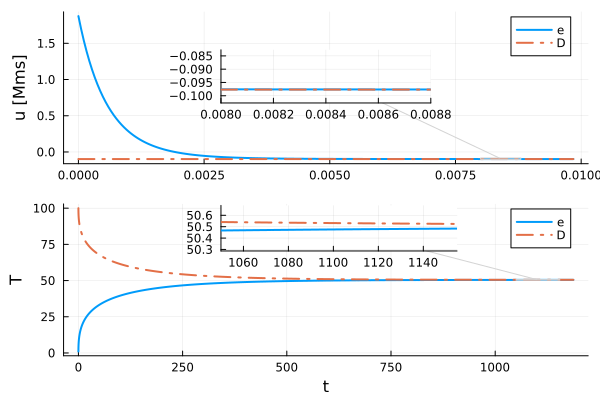
Figure 19: $e$-$D$ thermal and momentum equilibration with enforcing conservation: Average velocities and temperatures as function of time $t$ when $(n_{2},N_{0})=(7,7)$.

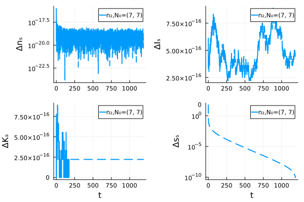
Figure 20: $e$-$D$ thermal and momentum equilibration with enforcing conservation when $T_{e}=1$ and $T_{D}=100$: Discrete conservation errors as functions of time when $(n_{2},N_{0})=(7,7)$.

Average velocities and temperatures of species $e$ and $D$ are plotted as function of time $t$ in Fig. 19. The zoomed in subplots in Fig. 19 show that correct equilibrium values of momentum and temperature are reached. As expected, the characteristic time of momentum relaxation time is significantly shorter than the characteristic time of temperature relaxation during electron-deuterium temperature and momentum equilibration process.

The time histories of the errors in discrete number density, momentum, energy conservation and entropy conservation are depicted in Fig. 20. As before, mass, momentum and energy conservation (102)-(104) are enforcing to the level of round-off error and H-theorem are preserved all the time, as demonstrated in Fig. 20. Fig. 21 illustrates that the local relative errors, $Error(\delta_{t}\hat{n})$, $Error(\delta_{t}\hat{I})$, and $Error(\delta_{t}\hat{K})$, during $e$-$D$ collision when $(n_{2},N_{0})=(7,7)$ are sufficiently small to satisfy the convergence criterion for conservation (83). As expected, the local relative errors of species $D$, with its larger mass, are smaller than those of species $e$. The convergence criterion $\delta_{t}\hat{T}$ (displayed in Eq. (50)) is approximately validity with a quite high precision, especially when $t\geq 10^{-2}$.

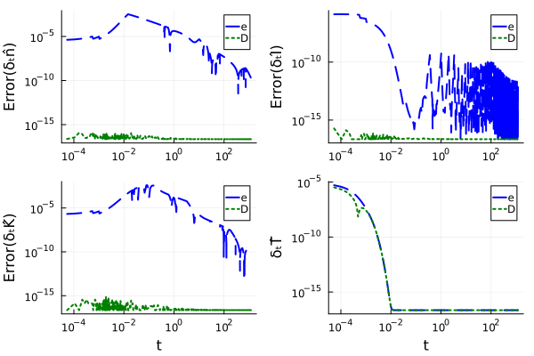
Figure 21: $e$-$D$ thermal and momentum equilibration with enforcing conservation when $T_{e}=1$ and $T_{D}=100$: Local errors of $\delta_{t}\hat{n}$, $\delta_{t}\hat{I}$, $\delta_{t}\hat{K}$ and convergence criterion $\delta_{t}\hat{T}$ as functions of time when $(n_{2},N_{0})=(7,7)$.

V.4 Three-species (e-D-alpha) thermal equilibration

Last test case is the three-species ($e$-$D$-$\alpha$) thermal equilibration which is an important problem in fusion plasma. In theory, the hot $\alpha$ particles in burning plasma will first exchange energy with electrons (of comparable $v_{th}$) and later thermalize with $D$ particles.

The simulation parameters are $m_{e}=1/1836$, $m_{D}=2$, $m_{\alpha}=4$, $-Z_{e}=Z_{D}=1$, $Z_{\alpha}=2$, $n_{e}=3$, $n_{D}=1$, $n_{\alpha}=1$. Initially $\hat{u}_{e}=\hat{u}_{D}=\hat{u}_{\alpha}=0$, $T_{e}=T_{D}=1$ and $T_{\alpha}=1750$, we choose $(n_{2},N_{0})=(7,7)$. In this case, $v_{eth}\approx 6.256\times 10^{-2}$, $v_{Dth}\approx 1.036\times 10^{-3}$ and $v_{\alpha th}\approx 3.065\times 10^{-2}$. The characteristic time $\tau_{0}$ is equivalent to the initial temperature relaxation time between $e$ and $D$, $\tau_{0}=1/\nu_{T}^{eD}$ where

$$\nu_{T}^{eD} \approx 441.72\times\frac{\sqrt{m_{e}m_{D}}\left(Z_{e}Z_{D}\right)^{2}n_{D}}{\left(m_{e}T_{D}+m_{D}T_{e}\right)^{3/2}}\ln{\Lambda_{eD}}\leavevmode\nobreak\ .$$ (112)

The maximum thermal velocity ratio, $v_{eth}/v_{Dth}\sim 60$. This case is solved with a self-adaptive timesteps and the number of timestep $N_{t}=710$.

Temperatures of all species as functions of time $t$ are plotted in Fig. 22. As anticipated, electrons heat up more rapidly than $D$ particles at early time when $t\leq 8$ (lower figure in Fig. 22). The $D$-$\alpha$ collision process can be observed for $t<300$ and finally, for $300<t<2000$, we can see that $\alpha$ and $D$ particles cool down while $e$ particles heat up. All the three species eventually reach the expected equilibrium temperature of $T_{\infty}=350.08$ (upper figure in Fig. 22).

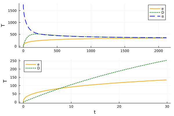
Figure 22: $e$-$D$-$\alpha$ thermal equilibration with enforcing conservation when $T_{e}=T_{D}=1$ and $T_{\alpha}=1750$: Temperature of the three species as functions of time (upper) and of $e$ and $D$ at the early time (lower) when $(n_{2},N_{0})=(7,7)$.

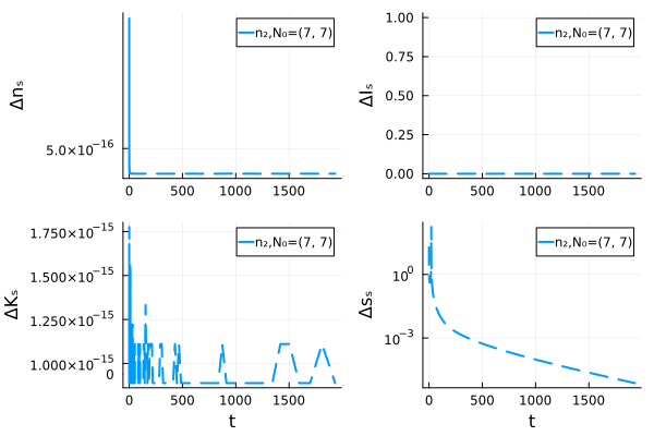
Figure 23: $e$-$D$-$\alpha$ thermal equilibration with enforcing conservation when $T_{e}=T_{D}=1$ and $T_{\alpha}=1750$: Discrete conservation errors as functions of time when $(n_{2},N_{0})=(7,7)$.

The time histories of the local errors in discrete number density, momentum, energy conservation and entropy conservation are plotted in Fig. 23. As expected, mass, momentum and energy conservation (102)-(104) are enforced to the level of round-off error, and H-theorem is preserved all the time, as shown in Fig. 23. The total local relative errors of $\delta_{t}\hat{n}$ and $\delta_{t}\hat{K}$ for all species as functions of time $t$ are plotted in Fig. 24. As we can see, the convergence criterion for conservation denoted by Eq. (83) is also satisfied for all sub-processes which are two-species collision.

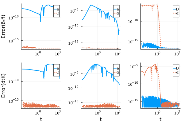
Figure 24: $e$-$D$-$\alpha$ thermal equilibration with enforcing conservation when $T_{e}=T_{D}=1$ and $T_{\alpha}=1750$: Local relative errors of $\delta_{t}\hat{n}$ and $\delta_{t}\hat{K}$ during all the two-species collision processes as functions of time when $(n_{2},N_{0})=(7,7)$.

VI Conclusion

In this study, we have developed an implicit meshfree algorithm for solving the multi-species nonlinear 0D-2V axisymmetric Fokker-Planck-Rosenbluth collision equation based on the Shkarofsky’s formula. The algorithm ensures mass, momentum, energy conservation and satisfies the H-theorem for general mass, temperature when average velocities are moderate. We construct an efficient meshfree algorithm based on the nonlinear Shkarofsky’s formula of FRP collision operator. Legendre polynomial expansion is employed in the angular direction which converges exponentially with the increment of number of the polynomials. King function expansion, a moment convergence method is utilized in the velocity axis. The kinetic moments will be computed by Romberg integration with high precision. Post-step projection to manifold method is used to enforce the conservations of the collision operators exactly.

The high accuracy of our algorithm is demonstrated by solving several typical problems in various non-equilibrium configurations. To handle the strong stiffness caused by the arbitrary disparity of mass and temperature, we implement interpolation between the different background meshgrids, which is also based on the King function. The fast convergence and high efficiency for various challenging problems have demonstrated the potential of our approach for multi-scale simulation of plasmas.

In order to fully realize the potential of the proposed approach for nonlinear, multi-scale plasma systems, we have extended the approach with self-adaptive background meshgrids, which will be discussed in a future publication. We finally remark that the present approach is efficient only for the system with no distinguishing asymmetries in the velocity space, for example, $\hat{u}_{a}\ll 1$. The first reason for this limitation is that the convergence rate of the Legendre polynomial expansions drops as the ratio of average velocity to thermal velocity increases. For example, $l=11$ when $\hat{u}_{a}=0.44$ while $l=3$ when $\hat{u}_{a}\leq 2.2\times 10^{-3}$. The second reason is that parameter $\hat{n}_{a_{s}}$, $\hat{u}_{a_{s}}$ and $\hat{v}_{{ath}_{s}}$ in the King function (54) may be dependent on $l$ when $\hat{u}_{a}\sim 1$, which is also under the development.

VII Acknowledgments

We would like to thank Peifeng Fan and Bojing Zhu for useful discussions. This work is supported by the GuangHe Foundation (ghfund202202018672), Collaborative Innovation Program of Hefei Science Center, CAS, (2021HSC-CIP019), National Magnetic Confinement Fusion Program of China (2019YFE03060000), Director Funding of Hefei Institutes of Physical Science from Chinese Academy of Sciences (Grant Nos. E25D0GZ5), and Geo-Algorithmic Plasma Simulator (GAPS) Project.

Appendix A King Function

When the velocity space is axisymmetric with $\hat{\boldsymbol{u}}_{a}=\hat{u}_{a}\mathbf{e}_{z}$, the Gaussian function will be:

$$\mathscr{G}\left(\hat{v},\mu\right)=\frac{\hat{n}_{a}}{\hat{v}_{ath}^{3}}\mathrm{e}^{-\left[\left(\hat{\boldsymbol{v}}-\hat{u}_{a}\mathbf{e}_{z}\right)/\hat{v}_{ath}\right]^{2}}.$$ (113)

The Gaussian function can be expanded based on Legendre polynomials as:

$$\mathscr{G}\left(\hat{v},\mu\right) = \sum_{l=0}^{\infty}\mathscr{G}_{l}^{0}\left(\hat{v}\right)\mathrm{P}_{l}^{0}\left(\mu\right)\leavevmode\nobreak\ .$$ (114)

The $l^{th}$-order amplitude, $\mathscr{G}_{l}^{0}\left(\hat{v}\right)$ can be calculated by the inverse transformation of Eq. (114), reads:

$$\mathscr{G}_{l}^{0}\left(\hat{v}\right) = \int_{-1}^{1}\mathscr{G}\left(\hat{v},\mu\right)\mathrm{P}_{l}^{0}(\mu)\mathrm{d}\mu,\quad l\in 0,1,\cdots,l_{M}\leavevmode\nobreak\ .$$ (115)

Substitute Eq. (113) into above equation, and after a tedious derivation process, one can obtain:

$$\mathscr{G}_{l}^{0}\left(\hat{v}\right) = \frac{\hat{n}_{a}}{(\hat{v}_{ath})^{3}}\sum_{m=0}^{l}C_{G_{l}}\frac{1}{\hat{\xi}_{a}^{m+1}}\left[(-1)^{m}\mathrm{e}^{-\left(\frac{\hat{v}-\hat{u}_{a}}{\hat{v}_{ath}}\right)^{2}}-(-1)^{l}\mathrm{e}^{-\left(\frac{\hat{v}+\hat{u}_{a}}{\hat{v}_{ath}}\right)^{2}}\right]\leavevmode\nobreak\ .$$ (116)

Here, $\hat{\xi}_{a}=2\hat{v}\hat{u}_{a}/\hat{v}_{ath}^{2}$ and

$$C_{G_{l}} = \frac{2l+1}{2}\frac{1}{2^{m}m!}\frac{(l+m)!}{(l-m)!}\leavevmode\nobreak\ .$$ (117)

The $l^{th}$-order King (54) function is in direct proportion to $\mathscr{G}_{l}^{0}$, reads:

$$\mathcal{K}_{l}\left(\hat{v};\hat{u}_{a},\hat{v}_{ath}\right) = \sqrt{\frac{1}{2\pi}}\frac{1}{\hat{n}_{a}}\mathscr{G}_{l}^{0}\left(\hat{v}\right)\leavevmode\nobreak\ .$$ (118)

The King function (54) has the following properties. When $v\to\infty$, the King function will be:

$$\lim_{v\to\infty}\mathcal{K}_{l}\left(v;\iota,\sigma\right)\to 0\leavevmode\nobreak\ .$$ (119)

When $\xi=2\iota v/\sigma^{2}\to 0$, the King function has the following asymptotic behaviour:

$$\lim_{\xi\to 0}\mathcal{K}_{l}\left(v;\iota,\sigma\right)=\sqrt{\frac{1}{2\pi}}\frac{\mathrm{e}^{-\sigma^{-2}\left(v^{2}+\iota^{2}\right)}}{(2l-1)!!}\frac{\xi^{l}}{\sigma^{3}}\left[1+\sum_{k=1}^{\infty}\frac{1}{2^{l}l!}\frac{(2l-1)!!}{(2l+2k+1)!!}\xi^{2k}\right]\leavevmode\nobreak\ .$$ (120)

In particular, $\xi\equiv 0$ gives:

$$\mathcal{K}_{l}\left(v;\iota,\sigma\right)\xlongequal[]{\xi=0}\delta_{l}^{0}\sqrt{\frac{1}{2\pi}}\frac{1}{\sigma^{3}}\mathrm{e}^{-\sigma^{-2}\left(v^{2}+\iota^{2}\right)}\leavevmode\nobreak\ .$$ (121)

Here, $\delta_{l}^{0}$ is the Kronecker symbol.

Appendix B Normalized FPRS collision operator

Substituting Eqs. (20)-(21), (31) and Eqs. (27)-(34) into Eq. (16), simplifying the result by combining the like terms gives the normalized FPRS collision operator in axisymmetric velocity space, reads:

$$\hat{\mathfrak{C}}_{ab}\left(\hat{\boldsymbol{v}},t\right) = 4\pi\sum_{i=0}^{9}\hat{\mathscr{S}}_{i}\leavevmode\nobreak\ .$$ (122)

The zero-order effect term owing to $\hat{F}$ in the collision term can be expressed as:

$$\hat{\mathscr{S}}_{0} = m_{M}\sum_{L=0}^{\infty}\hat{F}_{L}^{0}(\hat{v}_{ab},t)\mathrm{P}_{L}^{0}\times\sum_{l=0}^{\infty}\hat{f}_{l}^{0}(\hat{v},t)\mathrm{P}_{l}^{0}\leavevmode\nobreak\ .$$ (123)

The first-order effect terms owing to $\hat{H}_{L}^{0}$ will be:

$$\hat{\mathscr{S}}_{1} = C_{\hat{H}}\sum_{L=0}^{\infty}\mathrm{P}_{L}^{0}\frac{\partial}{\partial\hat{v}_{ab}}\hat{H}_{L}^{0}\times\sum_{l=0}^{\infty}\mathrm{P}_{l}^{0}\frac{\partial}{\partial\hat{v}}\hat{f}_{l}^{0},$$ (124)

$$\hat{\mathscr{S}}_{2} = C_{\hat{H}}\frac{1}{\hat{v}_{ab}}\sum_{L=1}^{\infty}\hat{H}_{L}^{0}\mathrm{P}_{L}^{1}\times\frac{1}{\hat{v}}\sum_{l=1}^{\infty}\hat{f}_{l}^{0}\mathrm{P}_{l}^{1}\leavevmode\nobreak\ .$$ (125)

Another first-order effect term, $\hat{\mathscr{S}}_{3}$ will be zero due to the derivatives related to the azimuth $\phi$ is zero. Especially, when $m_{a}=m_{b}$, the coefficient $C_{\hat{H}}\equiv 0$ which yields $\hat{\mathscr{S}}_{1}=\hat{\mathscr{S}}_{2}\equiv 0$ too. Similarly, the second-order effect terms owing to $\hat{G}_{L}^{0}$ will be:

$$\hat{\mathscr{S}}_{4} = C_{\hat{G}}\sum_{L=0}^{\infty}\mathrm{P}_{L}^{0}\frac{\partial^{2}}{\partial{\hat{\mathscr{v}}}^{2}}\hat{G}_{L}^{0}\times\sum_{l=0}^{\infty}\mathrm{P}_{l}^{0}\frac{\partial^{2}}{\partial{\hat{v}}^{2}}\hat{f}_{l}^{0},$$ (126)

$$\hat{\mathscr{S}}_{5} = 2C_{\hat{G}}\frac{1}{\hat{v}_{ab}}\sum_{L=1}^{\infty}\left(\frac{\hat{G}_{L}^{0}}{\hat{v}_{ab}}-\mathrm{P}_{L}^{0}\frac{\partial}{\partial\hat{v}_{ab}}\hat{G}_{L}^{0}\right)\times\frac{1}{\hat{v}}\sum_{l=1}^{\infty}\left(\frac{\hat{f}_{l}^{0}}{\hat{v}}-\mathrm{P}_{l}^{0}\frac{\partial}{\partial\hat{v}}\hat{f}_{l}^{0}\right)\mathrm{P}_{l}^{1},$$ (127)

$$\hat{\mathscr{S}}_{7} = C_{\hat{G}}\frac{1}{\hat{v}_{ab}}\sum_{L=0}^{\infty}\left(\mathrm{P}_{L}^{1,2}\frac{\hat{G}_{L}^{0}}{\hat{v}_{ab}}+\mathrm{P}_{L}^{0}\frac{\mathrm{\partial}\hat{G}_{L}^{0}}{\mathrm{\partial}\hat{\mathscr{v}}}\right)\times\frac{1}{\hat{v}}\sum_{l=0}^{\infty}\left(\mathrm{P}_{l}^{1,2}\frac{\hat{f}_{l}^{0}}{\hat{v}}+\mathrm{P}_{l}^{0}\frac{\mathrm{\partial}\hat{f}_{l}^{0}}{\mathrm{\partial}\hat{v}}\right),$$ (128)

$$\hat{\mathscr{S}}_{9} = C_{\hat{G}}\sum_{L=0}^{\infty}\left(\mathrm{P}_{L}^{1,\mu}\frac{\hat{G}_{L}^{0}}{\hat{v}_{ab}^{2}}+\mathrm{P}_{L}^{0}\frac{1}{\hat{v}_{ab}}\frac{\mathrm{\partial}\hat{G}_{L}^{0}}{\mathrm{\partial}\hat{\mathscr{v}}}\right)\times\sum_{l=0}^{\infty}\left(\mathrm{P}_{l}^{1,\mu}\frac{\hat{f}_{l}^{0}}{\hat{v}^{2}}+\mathrm{P}_{l}^{0}\frac{1}{\hat{v}}\frac{\mathrm{\partial}\hat{f}_{l}^{0}}{\mathrm{\partial}\hat{v}}\right)$$ (129)

where

$$\mathrm{P}_{l}^{1,\mu} = \frac{\mu}{\sqrt{1-\mu^{2}}}\mathrm{P}_{l}^{1},$$ (130)

$$\mathrm{P}_{l}^{1,2} = \mathrm{P}_{l}^{2}+\mathrm{P}_{l}^{1,\mu}\leavevmode\nobreak\ .$$ (131)

The rest second-order effect terms are zeros, $\hat{\mathscr{S}}_{6}=\hat{\mathscr{S}}_{8}=0$. As the above equations show, the FPRS collision operator (give in Eq. (122)) is a nonlinear model generally.

In particular, when the system is spherical symmetric in velocity space, the collision effect is independent on the angular direction of velocity space. Hence, the normalized FPRS collision operator (give in Eq. (122)) will be:

$$\hat{\mathscr{S}}_{0}\left(\hat{\boldsymbol{v}},t\right) = m_{M}\hat{F}{{}_{0}^{0}}(\hat{v}_{ab},t)\times\hat{f}_{0}^{0}(\hat{v},t),$$ (132)

$$\hat{\mathscr{S}}_{1}\left(\hat{\boldsymbol{v}},t\right) = C_{\hat{H}}\frac{\partial}{\partial\hat{v}_{ab}}\hat{H}{{}_{0}^{0}}\times\frac{\partial}{\partial\hat{v}}\hat{f}_{0}^{0},$$ (133)

$$\hat{\mathscr{S}}_{4}\left(\hat{\boldsymbol{v}},t\right) = C_{\hat{G}}\frac{\partial^{2}}{\partial{\hat{\mathscr{v}}}^{2}}\hat{G}{{}_{0}^{0}}\times\frac{\partial^{2}}{\partial{\hat{v}}^{2}}\hat{f}_{0}^{0},$$ (134)

$$\hat{\mathscr{S}}_{7}\left(\hat{\boldsymbol{v}},t\right) = \hat{\mathscr{S}}_{9}=C_{\hat{G}}\frac{1}{\hat{v}_{ab}}\frac{\partial}{\partial\hat{v}_{ab}}\hat{G}{{}_{0}^{0}}\times\frac{1}{\hat{v}}\frac{\partial}{\partial\hat{v}}\hat{f}_{0}^{0}\leavevmode\nobreak\ .$$ (135)

The remaining first-order effect terms and second-order effect terms will be zeros, $\hat{\mathscr{S}}_{2}=\hat{\mathscr{S}}_{3}=\hat{\mathscr{S}}_{5}=\hat{\mathscr{S}}_{6}=\hat{\mathscr{S}}_{8}=0$.

For self-collision process where $m_{M}=1$, the coefficients (give in Eq. (17)) will be consts, reads:

$$C_{\hat{F}}=4\pi,\quad C_{\hat{H}}=0,\quad C_{\hat{G}}=1/2\leavevmode\nobreak\ .$$ (136)

The normalized FPRS collision operator (give in Eqs. (122)-(135)) will further simplify to be a self-collision operator by substituting $\hat{F}_{L}^{0}$ and $\hat{v}_{ab}$ by $\hat{f}_{l}^{0}$ and $\hat{v}$ respectively.

Appendix C Convergence of King method

In backward Euler scheme, the first-order derivative, $\frac{\partial}{\partial t}f_{l}^{0}$ will be approximate as:

$$\frac{\partial}{\partial t}f_{l}^{0}{{}^{*}}(\hat{v}_{\alpha},t_{k}) = \frac{f_{l}^{0}{{}^{*}}(\hat{v}_{\alpha},t_{k+1})-f_{l}^{0}(\hat{v}_{\alpha},t_{k})}{\Delta t}+C{{}^{*}}\mathscr{O}(\Delta t^{2}),$$ (137)

$$\frac{\partial}{\partial t}f_{l}^{0}(\hat{v}_{\alpha},t_{k}) = \frac{f_{l}^{0}(\hat{v}_{\alpha},t_{k+1})-f_{l}^{0}(\hat{v}_{\alpha},t_{k})}{\Delta t}+C_{K}\mathscr{O}(\Delta t^{n}),\quad n\in\mathbb{Z}\leavevmode\nobreak\ .$$ (138)

Here, parameters $C^{*}$ and $C_{K}$ are constants. Substituting above equations into Eqs. (110)-(109) gives:

$$C_{2} = \frac{f_{l}^{0}{{}^{*}}(\hat{v}_{\alpha},t_{k+1})-f_{l}^{0}(\hat{v}_{\alpha},t_{k})+f_{l}^{0}(\hat{v}_{\alpha},t_{k})-f_{l}^{0}(\hat{v}_{\alpha},t_{k+1})}{\Delta t^{3}\times f_{l}^{0}{{}^{*}}(\hat{v}_{\alpha},t_{k+1})},$$ (139)

$$C_{0} = \frac{1}{\Delta t}\frac{f_{l}^{0}{{}^{*}}(\hat{v}_{\alpha},t_{k+1})-f_{l}^{0}(\hat{v}_{\alpha},t_{k})+f_{l}^{0}(\hat{v}_{\alpha},t_{k})-f_{l}^{0}(\hat{v}_{\alpha},t_{k+1})}{\frac{\partial}{\partial t}f_{l}^{0}{{}^{*}}(\hat{v}_{\alpha},t_{k})-C^{*}\mathscr{O}(\Delta t^{2})}\leavevmode\nobreak\ .$$ (140)

That is:

$$C_{2} = \frac{\frac{\partial}{\partial t}f_{l}^{0}{{}^{*}}(\hat{v}_{\alpha},t_{k})-\frac{\partial}{\partial t}f_{l}^{0}(\hat{v}_{\alpha},t_{k})+C_{K}\mathscr{O}(\Delta t^{n})-C^{*}\mathscr{O}(\Delta t^{2})}{\Delta t^{2}\times f_{l}^{0}{{}^{*}}(\hat{v}_{\alpha},t_{k+1})},$$ (141)

$$C_{0} = 1-\frac{\frac{\partial}{\partial t}f_{l}^{0}(\hat{v}_{\alpha},t_{k})-C_{K}\mathscr{O}(\Delta t^{n})}{\frac{\partial}{\partial t}f_{l}^{0}{{}^{*}}(\hat{v}_{\alpha},t_{k})-C^{*}\mathscr{O}(\Delta t^{2})}\leavevmode\nobreak\ .$$ (142)

With assumption $\frac{\partial}{\partial t}f_{l}^{0}(\hat{v}_{\alpha},t_{k})=C_{v}(\hat{v}_{\alpha})\frac{\partial}{\partial t}f_{l}^{0}{{}^{*}}(\hat{v}_{\alpha},t_{k})$ where $C_{v}(\hat{v}_{\alpha})$ is a constant, we obtain:

$$C_{2} = \frac{(1-C_{v})\frac{\partial}{\partial t}f_{l}^{0}{{}^{*}}(\hat{v}_{\alpha},t_{k})+C_{K}\mathscr{O}(\Delta t^{n})-C^{*}\mathscr{O}(\Delta t^{2})}{\Delta t^{2}\times f_{l}^{0}{{}^{*}}(\hat{v}_{\alpha},t_{k+1})},$$ (143)

$$C_{0} = 1-\frac{C_{v}\frac{\partial}{\partial t}f_{l}^{0}{{}^{*}}(\hat{v}_{\alpha},t_{k})-C_{K}\mathscr{O}(\Delta t^{n})}{\frac{\partial}{\partial t}f_{l}^{0}{{}^{*}}(\hat{v}_{\alpha},t_{k})-C^{*}\mathscr{O}(\Delta t^{2})}\leavevmode\nobreak\ .$$ (144)

Substituting $\frac{\partial}{\partial t}f_{l}^{0}{{}^{*}}=C_{0}{{}^{*}}+C{{}^{*}}\mathscr{O}(\Delta t^{2})$ into above two equations leads to:

$$C_{2} = \frac{(1-C_{v})C_{0}{{}^{*}}+C_{K}\mathscr{O}(\Delta t^{n})-C_{v}C^{*}\mathscr{O}(\Delta t^{2})}{\Delta t^{2}\times f_{l}^{0}{{}^{*}}(\hat{v}_{\alpha},t_{k+1})},$$ (145)

$$C_{0} = (1-C_{v})-\frac{C_{v}C{{}^{*}}\mathscr{O}(\Delta t^{2})-C_{K}\mathscr{O}(\Delta t^{n})}{C_{0}{{}^{*}}}\leavevmode\nobreak\ .$$ (146)

Eq. (146) denotes parameter $C_{0}$ is a constant at single node of velocity axis.

References

- Rosenbluth et al. (1957) M. N. Rosenbluth, W. M. MacDonald, and D. L. Judd, Physical Review 107, 1 (1957).
- Taitano et al. (2015a) W. T. Taitano, L. Chacón, A. N. Simakov, and K. Molvig, Journal of Computational Physics 297, 357 (2015a).
- Shkarofsky (1963) I. P. Shkarofsky, Canadian Journal of Physics 41, 1753 (1963).
- Shkarofsky et al. (1967) I. P. Shkarofsky, T. W. Johnston, M. P. Bachynski, and J. L. Hirshfield, American Journal of Physics 35, 551 (1967).
- Landau (1937) L. D. Landau, Zh. Eksper. i Theoret. Fiz. 7 (2) (1937).
- Vlasov (1968) A. A. Vlasov, Soviet Physics Uspekhi 10, 721 (1968).
- Boltzmann (1872) V. L. Boltzmann, Wissenschaftliche Abhandlungen (1872).
- Chang and Cooper (1970) J. Chang and G. Cooper, Journal of Computational Physics 6, 1 (1970).
- Taitano et al. (2016) W. T. Taitano, L. Chacón, and A. N. Simakov, Journal of Computational Physics 318, 391 (2016).
- Thomas et al. (2012) A. G. Thomas, M. Tzoufras, A. P. Robinson, R. J. Kingham, C. P. Ridgers, M. Sherlock, and A. R. Bell, Journal of Computational Physics 231, 1051 (2012).
- Bell et al. (2006) A. R. Bell, A. P. Robinson, M. Sherlock, R. J. Kingham, and W. Rozmus, Plasma Physics and Controlled Fusion 48 (2006), 10.1088/0741-3335/48/3/R01.
- Johnston (1960) T. W. Johnston, Physical Review 120, 1103 (1960).
- Shkarofsky (1997) I. P. Shkarofsky, Physics of Plasmas 4, 2464 (1997).
- Kingham and Bell (2004) R. J. Kingham and A. R. Bell, Journal of Computational Physics 194, 1 (2004).
- Thomas et al. (2009) A. G. Thomas, R. J. Kingham, and C. P. Ridgers, New Journal of Physics 11 (2009), 10.1088/1367-2630/11/3/033001.
- Robinson et al. (2008) A. P. Robinson, M. Sherlock, and P. A. Norreys, Physical Review Letters 100, 1 (2008).
- Tzoufras et al. (2011) M. Tzoufras, A. R. Bell, P. A. Norreys, and F. S. Tsung, Journal of Computational Physics 230, 6475 (2011).
- Tzoufras et al. (2013) M. Tzoufras, A. Tableman, F. S. Tsung, W. B. Mori, and A. R. Bell, Physics of Plasmas 20 (2013), 10.1063/1.4801750.
- Wu et al. (2013) S. Z. Wu, H. Zhang, C. T. Zhou, S. P. Zhu, and X. T. He, in EPJ Web of Conferences, Vol. 59 (2013).
- Mijin et al. (2020) S. Mijin, F. Militello, S. Newton, J. Omotani, and R. J. Kingham, Plasma Physics and Controlled Fusion 62 (2020), 10.1088/1361-6587/ab9b39.
- Krook and Wu (1977) M. Krook and T. T. Wu, Physics of Fluids 20, 1589 (1977).
- Bell et al. (1981) A. R. Bell, R. G. Evans, and D. J. Nicholas, Physical Review Letters 46, 243 (1981).
- Matte and Virmont (1982) J. P. Matte and J. Virmont, Physical Review Letters 49, 1936 (1982).
- Shkarofsky et al. (1992) I. P. Shkarofsky, M. M. Shoucri, and V. Fuchs, Computer Physics Communications 71, 269 (1992).
- Alouani-Bibi et al. (2004) F. Alouani-Bibi, M. M. Shoucri, and J. P. Matte, Computer Physics Communications 164, 60 (2004).
- Zhao et al. (2018) B. Zhao, G. Y. Hu, J. Zheng, and Y. Ding, High Energy Density Physics 28, 1 (2018).
- Wu et al. (2011) S. Wu, C. Zhou, S. Zhu, H. Zhang, and X. He, Physics of Plasmas 18 (2011), 10.1063/1.3553452.
- Pareschi et al. (2000) L. Pareschi, G. Russo, and G. Toscani, Journal of Computational Physics 165, 216 (2000).
- Filbet and Pareschi (2002) F. Filbet and L. Pareschi, Journal of Computational Physics 179, 1 (2002).
- Pataki and Greengard (2011) A. Pataki and L. Greengard, Journal of Computational Physics 230, 7840 (2011).
- Askari and Adibi (2015) M. Askari and H. Adibi, Ain Shams Engineering Journal 6, 1211 (2015).
- Morton K. W. and Mayyers David (2005) Morton K. W. and Mayyers David, Cambridge University Press, Vol. 54 (Cambridge University Press, 2005) p. 293.
- Li et al. (2021) R. Li, Y. Ren, and Y. Wang, Journal of Computational Physics 434 (2021), 10.1016/j.jcp.2021.110235.
- Press et al. (2007) W. H. Press, S. A. Teukolsky, W. T. Verrerlling, and F. B. P., Numerical Recipes (Cambridge University Press, 2007) p. 1262.
- Taitano et al. (2015b) W. T. Taitano, D. A. Knoll, and L. Chacón, Journal of Computational Physics 284, 737 (2015b).
- Taitano et al. (2017) W. T. Taitano, L. Chacón, and A. N. Simakov, Journal of Computational Physics 339, 453 (2017).
- Daniel et al. (2020) D. Daniel, W. T. Taitano, and L. Chacón, Computer Physics Communications 254, 107361 (2020).
- Saad (2003) Y. Saad, Iterative Methods for Sparse Linear Systems, Second Edition (2003) p. 528.
- Courant et al. (1986) R. Courant, K. Friedrichs, and H. Lewy, “Über die partiellen differenzengleichungen der mathematischen physik,” (Birkhäuser Boston, 1986) pp. 53–95.
- Larroche (2003) O. Larroche, The European Physical Journal D - Atomic, Molecular and Optical Physics 27, 131 (2003).
- E. et al. (2006) H. E., W. G., and L. C., Geometric Numerical Integration, Vol. 31 (Springer-Verlag, 2006) pp. 805–882.
- Moore and Reich (2003) B. Moore and S. Reich, Numerische Mathematik 95, 625 (2003).
- Reich (1999) S. Reich, SIAM Journal on Numerical Analysis 36, 1549 (1999).
- Rackauckas and Nie (2017) C. Rackauckas and Q. Nie, Journal of Open Research Software 5, 15 (2017).
- Bauer (1961) F. L. Bauer, Communications of the ACM 4, 255 (1961).
- Hairer (1999) E. Hairer, Numerische Mathematik 84, 199 (1999).
- Huba (2011) J. D. Huba, NRL PLASMA FORMULARY (NRL, 2011) pp. 1–71.
- Braginskii (1965) S. Braginskii, Reviews of Plasma Physics 1, 205 (1965).
- Robson and Ness (1986) R. E. Robson and K. F. Ness, Physical Review A 33, 2068 (1986).
- Sunahara et al. (2003) A. Sunahara, J. A. Delettrez, C. Stoeckl, R. W. Short, and S. Skupsky, Physical Review Letters 91, 1 (2003).
- Joglekar et al. (2018) A. S. Joglekar, B. J. Winjum, A. Tableman, H. Wen, M. Tzoufras, and W. B. Mori, Plasma Physics and Controlled Fusion 60 (2018), 10.1088/1361-6587/aab978.
- Fornberg (1998) B. Fornberg, SIAM Review 40, 685 (1998).
- Fong and Saunders (2011) D. C.-L. Fong and M. Saunders, SIAM Journal on Scientific Computing 33, 2950 (2011).
- Wright and Holt (1985) S. J. Wright and J. N. Holt, The Journal of the Australian Mathematical Society. Series B. Applied Mathematics 26, 387 (1985).
- Kanzow et al. (2004) C. Kanzow, N. Yamashita, and M. Fukushima, Journal of Computational and Applied Mathematics 172, 375 (2004).
- Braginskii (1958) S. I. Braginskii, J. Exptl. Theoret. Phys. (U.S.S.R.) 6, 459 (1958).
- Fornberg (1996) B. Fornberg, A Practical Guide to Pseudospectral Methods (Cambridge University Press, 1996).