FIVB ranking: Misstep in the right direction

Abstract

This work uses a statistical framework to present and evaluate the ranking algorithm that has been used by Fédération Internationale de Volleyball (FIVB) since 2020. The salient feature of the FIVB ranking is the use of the probabilistic model, which explicitly calculates the probabilities of the games to come. This explicit modeling is new in the context of official ranking, and we study the optimality of its parameters as well as its relationship with the ranking algorithm as such. The analysis is carried out using both analytical and numerical methods. We conclude that, from the modeling perspective, the use of the home-field advantage (HFA)would be beneficial and that the weighting of the game results is counterproductive. Regarding the algorithm itself, we explain the rationale beyond the approximations currently used and explain how to find new parameters which improve the performance. Finally, we propose a new model that drastically simplifies both the implementation and interpretation of the resulting algorithm.

1 Introduction

The ranking of teams/players is one of the fundamental problems in competitive sports and is used, for example, to declare the champion or to promote and relegate the teams between leagues. In general terms, the ranking is meant to reflect the relative strength of the teams/players, and should have some forecasting capabilities, i.e., to allow one to predict the game results which may be useful for organizing well-balanced tournaments (Csató, 2024).

In this work, we present and evaluate the ranking algorithm, used by the Fédération Internationale de Volleyball (FIVB). Our study is motivated by the modern approach adopted by the FIVB, where six outcomes of the volleyball games have explicit probabilistic models defined in FIVB (2024). To our best knowledge, this is the first officially adopted ranking algorithm to use such an approach and, merely due to this fact, deserves attention in sport analytics. Of course, international volleyball is also a popular sport, and understanding its rating strategy is interesting on its own merit.

The FIVB ranking adopted in 2020 can be classified as power-ranking, where teams are assigned a real-valued parameter called skills (also known as strength or power) and the teams are ranked (ordered) by sorting the skills. This approach departs from the more conventional ranking based on counting of the points associated with the results of the games, and is often considered to be more “fair”.

The power-ranking approach was already adopted by the Fédération Internationale de Football Association (FIFA) to rank the Men’s and Women’s teams, and the analysis made by Szczecinski and Roatis (2022) revealed its strength and showed possible improvements. One of the criticisms of the FIFA ranking made in Szczecinski and Roatis (2022) is that, being based on the Elo rating Elo (2008), it inherits its main drawback, i.e., the lack of an explicit probabilistic model of the game outcomes Szczecinski and Djebbi (2020). From a statistical perspective, this lack of forecasting capability is, indeed, a significant drawback which makes it difficult to evaluate the ranking objectively.

In this regard, the FIVB ranking proposes a radical and modern approach: each of the six outcomes of the volleyball game is assigned a probability that is calculated from the skills (known before the game) using the so-called Cumulative Link (CL) model (Tutz, 2012, Ch. 9.1).

The objective of this work is to present the FIVB ranking in a statistical framework, propose the evaluation methodology, and analyze the optimality of the algorithm’s parameters. Since there are many sports whose games end with multiple outcomes (i.e., more than two), understanding how ranking algorithms may be constructed in such cases will be useful beyond the context of the FIVB ranking.

This work is organized as follows: in Sec. 2, we cast the ranking in the inference context, where the goal is to estimate the skills from the outcomes of the games. This allows us to understand the relationship between the probabilistic model and the ranking algorithm as such. The parameters of the model are assessed in Sec. 3, where, both the analytical and numerical approaches are applied to evaluate the importance of the thresholds in the CL model, the numerical scores used in the FIVB algorithms, the role of the home-field advantage (HFA), and the utility of weights associated with games’ categories. In Sec. 4 we show that, using a logistic function in the CL model (instead of the Gaussian cumulative density function (CDF), currently defined in the FIVB ranking) produces a new, easy to interpret ranking algorithm which, moreover, does not need auxiliary numerical scores which are required in the current FIVB ranking.

We terminate the work in Sec. 6 summarizing the finding and showing the recommended changes to the FIVB ranking algorithm. Overall, we conclude that, from the statistical perspective, using an explicit probabilistic model to build a ranking algorithm is a step in the right direction. On the other hand, we qualify it as misstep because many approximations lead to sub-optimality, which might have been easily avoided.

2 Model and ranking

Consider the scenario, where, of the $M$ teams, two are selected to face each other in a game. The games are indexed with $t=1,2,\ldots,T$. Teams are indexed with a pair $(i_{t},j_{t})$, where $i_{t},j_{t}\in\{1,\ldots,M\}$. The team $i_{t}$ is called the home-team, and the team $j_{t}$ - the away-team. We keep this naming convention even when a game is played on a neutral venue.

The outcome of the $t$-th game $y_{t}\in\mathcal{Y}$ is ordinal in nature, with meaning such as “significance”, which has no numerical value but may be ordered, and, for convenience, we index it with natural numbers $\mathcal{Y}=\{0,\ldots,L-1\}$ in decreasing significance order, i.e., the outcome $y=0$ is the most important and $y=L-1$ is the least important one, where the significance is evaluated from the point of view of the home team $i_{t}$. Quite naturally, the most significant outcome for the home team is the least significant for the away team.

In particular, volleyball games, which we will be interested in, produce $L=6$ possible outcomes “3-0”, “3-1”, “3-2”, “2-3”, “1-3”, “0-3”, where “$k$-$l$” means that the home team won $k$ sets and the away team won $l$ sets; i.e., the first three results mean that the home team won. For the purpose of the derivations, we use indices $y\in\mathcal{Y}$, but it is easier to understand the meaning of the explicit results in the form “$k$-$l$”; i.e., the result $y_{t}=0$ corresponds to the outcome “3-0”, $y_{t}=1$ – to “3-1”, and $y_{t}=5$ – to “0-3”. We will use both and it should not lead to any confusion.

2.1 Rating as statistical inference

The goal of the ranking is to order the teams and, to this end, we assume that they are characterized by intrinsic parameters called “skills” $\theta_{m}\in\mathbb{R},m=1,\ldots,M$. Then, by inferring the skills $\boldsymbol{\theta}=[\theta_{1},\ldots,\theta_{M}]^{\mathsf{T}}$ from the observed outcomes of the games $\boldsymbol{y}=[y_{1},\ldots,y_{T}]^{\mathsf{T}}$, and ordering them, the ranking is naturally obtained.

Arguably the most popular probabilistic model of the relationship between the skills $\boldsymbol{\theta}$, and the random variable $Y_{t}$ (which models $y_{t}$) links the latter to the difference between the skills of the home and away teams:

$$\Pr\left\{Y_{t}=y|\boldsymbol{\theta},\boldsymbol{x}_{t}\right\} =\mathsf{P}_{y}(z_{t}),$$ (1)

$$z_{t} =\boldsymbol{x}_{t}^{\mathsf{T}}\boldsymbol{\theta},$$ (2)

where $\mathsf{P}_{y}(z)$ is defined to strike balance between the complexity of the inference procedure and the modeling flexibility (that is, ability of the model (1) to fit the observations). Also, for compactness of notation, we introduce the scheduling vector

$$\boldsymbol{x}_{t}=[x_{1,t},\ldots,x_{M,t}]^{\mathsf{T}},$$ (3)

where $x_{i_{t},t}=1$, $x_{j_{t},t}=-1$, and $x_{m,t}=0$ for $m\notin\{i_{t},j_{t}\}$.

With the model defined, we may use conventional estimation strategies. For example, the maximum a posteriori (MAP) estimate of $\boldsymbol{\theta}$ is obtained solving

$$\hat{\boldsymbol{\theta}} =\mathop{\mathrm{argmax}}_{\boldsymbol{\theta}}\log f\Big{(}\boldsymbol{\theta}\big{|}\{y_{t},\boldsymbol{x}_{t}\}_{t=1}^{T}\Big{)}$$ (4)

$$=\mathop{\mathrm{argmin}}_{\boldsymbol{\theta}}\sum_{t=1}^{T}\ell_{y_{t}}(z_{t})+\rho(\boldsymbol{\theta}),$$ (5)

where we use the common assumption that $Y_{t},t=1,\ldots,T$ are independent when conditioned on $\boldsymbol{x}_{t}$ and $\boldsymbol{\theta}$, the negated log-score

$$\ell_{y}(z) =-\log\mathsf{P}_{y}(z),$$ (6)

is a convenient representation of probability in log domain, and the prior distribution of the skills is defined via $\rho(\boldsymbol{\theta})=-\log f(\boldsymbol{\theta})$.

For example, in the simple case of binary win/loss games $y_{t}\in\{0,1\}$, we may adopt the logistic model,

$$\mathsf{P}_{y}(z) =\mathcal{L}\big{(}(-1)^{y}z\big{)},\quad y=0,1$$ (7)

$$\mathcal{L}(z) =\frac{1}{1+\mathrm{e}^{-z}},$$ (8)

and use the Gaussian prior for $\theta_{m}$,

$$f(\theta_{m}) =\mathcal{N}\Big{(}\theta;0,\frac{1}{\gamma}\Big{)}$$ (9)

where

$$\mathcal{N}(z;\mu,v)=\frac{1}{\sqrt{2\pi v}}\exp\Big{(}-\frac{1}{2v}(z-\mu)^{2}\Big{)}$$ (10)

is the Gaussian probability density function (PDF). Then,

$$\rho(\boldsymbol{\theta}) =\frac{1}{2}\gamma\|\boldsymbol{\theta}\|^{2}+{\textnormal{Const.}},$$ (11)

and, by finding $\hat{\boldsymbol{\theta}}$ in (4) we implement a logistic regression with $L_{2}$ regularization.

A more general formulation is obtained by rewriting (5) as

$$\hat{\boldsymbol{\theta}} =\mathop{\mathrm{argmin}}_{\boldsymbol{\theta}}J(\boldsymbol{\theta})$$ (12)

$$J(\boldsymbol{\theta}) =\sum_{t=1}^{T}\ell^{{\textnormal{loss}}}_{y_{t}}(\boldsymbol{x}^{\mathsf{T}}_{t}\boldsymbol{\theta})+\rho(\boldsymbol{\theta}),$$ (13)

where we use the “loss function” $\ell^{{\textnormal{loss}}}_{y}(z)$ which may, but does not need to, be the same as the log-score $\ell_{y}(z)$ in (6). As we shall see, to simplify calculations, the loss function may be a proxy of the log-score. In this “machine learning” formulation, $\rho(\boldsymbol{\theta})$ is called a regularization function.

Stochastic gradient rating

While (12) provides a conceptual reference framework to analyze the models used for rating and can be applied with a moderate value of $T$ (when it is reasonable to assume that the skills do not change significantly), the online (real-time) rating, where the skills are updated after each game, is more common in practice.

To obtain such a rating algorithm from the previous formulation, it enough to set $\rho(\boldsymbol{\theta})=0$, and solve (12) using the stochastic gradient (SG) algorithm, defined as follows:

$$\hat{\boldsymbol{\theta}}_{t+1} =\hat{\boldsymbol{\theta}}_{t}-\mu\big{[}\nabla_{\boldsymbol{\theta}}\ell^{{\textnormal{loss}}}_{y_{t}}(\boldsymbol{x}_{t}^{\mathsf{T}}\boldsymbol{\theta})\big{]}_{\boldsymbol{\theta}=\hat{\boldsymbol{\theta}}_{t}}$$ (14)

$$=\hat{\boldsymbol{\theta}}_{t}-\mu\boldsymbol{x}_{t}\dot{\ell}^{{\textnormal{loss}}}_{y_{t}}(\boldsymbol{x}_{t}^{\mathsf{T}}\hat{\boldsymbol{\theta}}_{t}),$$ (15)

where $\mu$ is the adaptation step, and

$$\dot{\ell}^{{\textnormal{loss}}}_{y}(z) =\frac{\,\mathrm{d}}{\,\mathrm{d}z}\ell^{{\textnormal{loss}}}_{y}(z).$$ (16)

The algorithm is initialized with $\boldsymbol{\theta}_{0}$, e.g., with $\boldsymbol{\theta}_{0}=[0,\ldots,0]^{\mathsf{T}}$.

When $\ell^{{\textnormal{loss}}}_{y}(z)$ is convex in $z$, for sufficiently large $t$ and appropriately chosen $\mu$, the solution of (15) approximates “well” $\hat{\boldsymbol{\theta}}$. The adaptation step, $\mu$, trades off the convergence speed (which tells how quickly, with $t$, $\hat{\boldsymbol{\theta}}_{t}$ approaches $\hat{\boldsymbol{\theta}}$) against the accuracy (which measures how far $\hat{\boldsymbol{\theta}}_{t}$ is from $\hat{\boldsymbol{\theta}}$). Although this is, admittedly, a vague statement, the precise analysis of the SG solution is not trivial even if some light is shed on this issue, e.g., in Aldous (2017), Jabin and Junca (2015), Szczecinski and Roatis (2022), Gomes de Pinho Zanco et al. (2024). In fact, (Szczecinski and Roatis, 2022, Sec. 3.3) shows that (15) may be seen as an approximation of a nonlinear Kalman filter, which estimates skills at time $t$ from previous observations $y_{1},\ldots,y_{t-1}$.

In this perspective, the skills $\hat{\boldsymbol{\theta}}_{t}$ are approximate solutions to the maximum likelihood (ML) estimation of the skills $\boldsymbol{\theta}$: the approximation is due to the use of the stochastic gradient and due to the use of the loss function, which may approximate the log-score.

Scale

It turns out that the skills estimates, $\hat{\theta}_{m}$ ($\hat{\theta}_{m,t}$ in case of the SG algorithm (15)), may be quite small and therefore, to place them in a comfortable range (e.g., for visual interpretation by the users), we may multiply them by an arbitrarily chosen scale $s>0$, i.e., making the change of variables $\boldsymbol{\theta}^{\prime}=s\boldsymbol{\theta}$. This scale change can be made directly on the final solutions in (12), as $\hat{\boldsymbol{\theta}}^{\prime}=s\hat{\boldsymbol{\theta}}$ or in (15), as $\hat{\boldsymbol{\theta}}^{\prime}_{t}=s\hat{\boldsymbol{\theta}}_{t}$. In fact, the latter can be integrated into the recursive equation yielding

$$\hat{\boldsymbol{\theta}}^{\prime}_{t+1} =\hat{\boldsymbol{\theta}}^{\prime}_{t}-\mu s\boldsymbol{x}_{t}\dot{\ell}^{{\textnormal{loss}}}_{y_{t}}(\boldsymbol{x}_{t}^{\mathsf{T}}\hat{\boldsymbol{\theta}}^{\prime}_{t}/s).$$ (17)

Home-field advantage (HFA)and weighting
We assumed that the probabilistic model (1) depends only on $z_{t}=\boldsymbol{x}^{\mathsf{T}}_{t}\boldsymbol{\theta}$ and the outcome $y_{t}$. However, a more general approach may be used in which other exogenous variables affect the model.

For example, we may want to take into account the HFA using a binary variable $h_{t}\in\{0,1\}$ that indicates whether the game $t$ is played on the home venue, i.e., in the country of the team $i_{t}$, (then $h_{t}=1$), or is played in the neutral venue (when $h_{t}=0$). The popular model relies on boosting the skills of the home team, or, equivalently, on increasing the values of $z_{t}$ by the HFA parameter $\eta$, i.e.,

$$\ell^{{\textnormal{loss}}}_{y_{t},h_{t}}(z_{t})=\ell^{{\textnormal{loss}}}_{y_{t}}(z_{t}+h_{t}\eta);$$ (18)

the exogenous variable $h_{t}$ is shown as a subscript, and $\eta$ is a part of the model.

Using the same notation, we may modify the loss function via heuristics, such as weighting

$$\ell^{{\textnormal{loss}}}_{y_{t},v_{t}}(z_{t}) =\xi_{v_{t}}\ell^{{\textnormal{loss}}}_{y_{t}}(z_{t})$$ (19)

where $v_{t}$ is a categorical variable associated with game $t$, $v_{t}\in\{0,\ldots,K-1\}$, and the weight $\xi_{v}\geq 0$ allows us to modulate the relative importance of the term $\ell^{{\textnormal{loss}}}_{y}(z)$: the smaller $\xi_{v_{t}}$ is, the less impact the pair $(z_{t},y_{t})$ will have on the solution $\hat{\boldsymbol{\theta}}$.

In the rating context, $v_{t}$ is called the “prestige” of the game (in the FIVB ranking) or its “importance” (in the FIFA ranking).

The weights $\boldsymbol{\xi}=[\xi_{0},\ldots,\xi_{K-1}]$ are then subjectively defined by experts. Note that, multiplying all the terms under optimization (12) by a positive constant does not change the optimization results, therefore, without loss of generality, we may set $\xi_{0}=1$.

Although subjective weighting is not uncommon in statistical literature, see e.g., Hu and Zidek (2001), Ley et al. (2019), it is possible to evaluate the weighting objectively. For example, Szczecinski and Roatis (2022) concluded that the use of weighting is counterproductive in the FIFA ranking.

2.2 FIVB rating algorithm

The FIVB ranking defines (1)

$$\mathsf{P}^{{\textnormal{FIVB}}}_{y}(z) =\mathsf{P}_{y}(z;\boldsymbol{c}^{{\textnormal{FIVB}}})$$ (20)

using the so-called CL model (Tutz, 2012, Ch. 9.1)

$$\mathsf{P}_{y}(z;\boldsymbol{c}) =\Phi(z+c_{y})-\Phi(z+c_{y-1}),\quad y=0,\ldots,L-1,$$ (21)

where $\Phi(z)=\frac{1}{\sqrt{2\pi}}\int_{-\infty}^{z}\exp(-0.5v^{2})\,\mathrm{d}v$ is the CDF of a zero-mean, unit-variance Gaussian distribution. The model is parameterized with thresholds $\boldsymbol{c}=[c_{-1},c_{0},\ldots,c_{L-1}]$, which are monotonically increasing with $l$, and, to simplify the discussion, may also be assumed symmetric, i.e.,

$$c_{l}=-c_{L-2-l},$$ (22)

and always set the first, and the last thresholds as $c_{-1}=-c_{L-1}=-\infty$.

The FIVB ranking defined the thresholds as follows:

$$c^{{\textnormal{FIVB}}}_{0}=-c^{{\textnormal{FIVB}}}_{4}=-1.06, c^{{\textnormal{FIVB}}}_{1}=-c^{{\textnormal{FIVB}}}_{3}=-0.394, c^{{\textnormal{FIVB}}}_{3}=0.$$ (23)

The symmetry of the thresholds $c^{{\textnormal{FIVB}}}_{y}=-c^{{\textnormal{FIVB}}}_{L-2-y}$, and of the CDF, $\Phi(z)=1-\Phi(-z)$, yields the symmetric forms $\mathsf{P}^{{\textnormal{FIVB}}}_{y}(z)=\mathsf{P}^{{\textnormal{FIVB}}}_{L-1-y}(-z)$, as can be appreciated in Fig. 1. One of the properties of the CL model is that the probability of the outcome “not less important than $y$” is calculated as

$$\Pr\left\{Y\leq y|z\right\}=\sum_{l=0}^{y}\mathsf{P}^{{\textnormal{FIVB}}}_{l}(z)=\Phi(z+c^{{\textnormal{FIVB}}}_{y}).$$ (24)

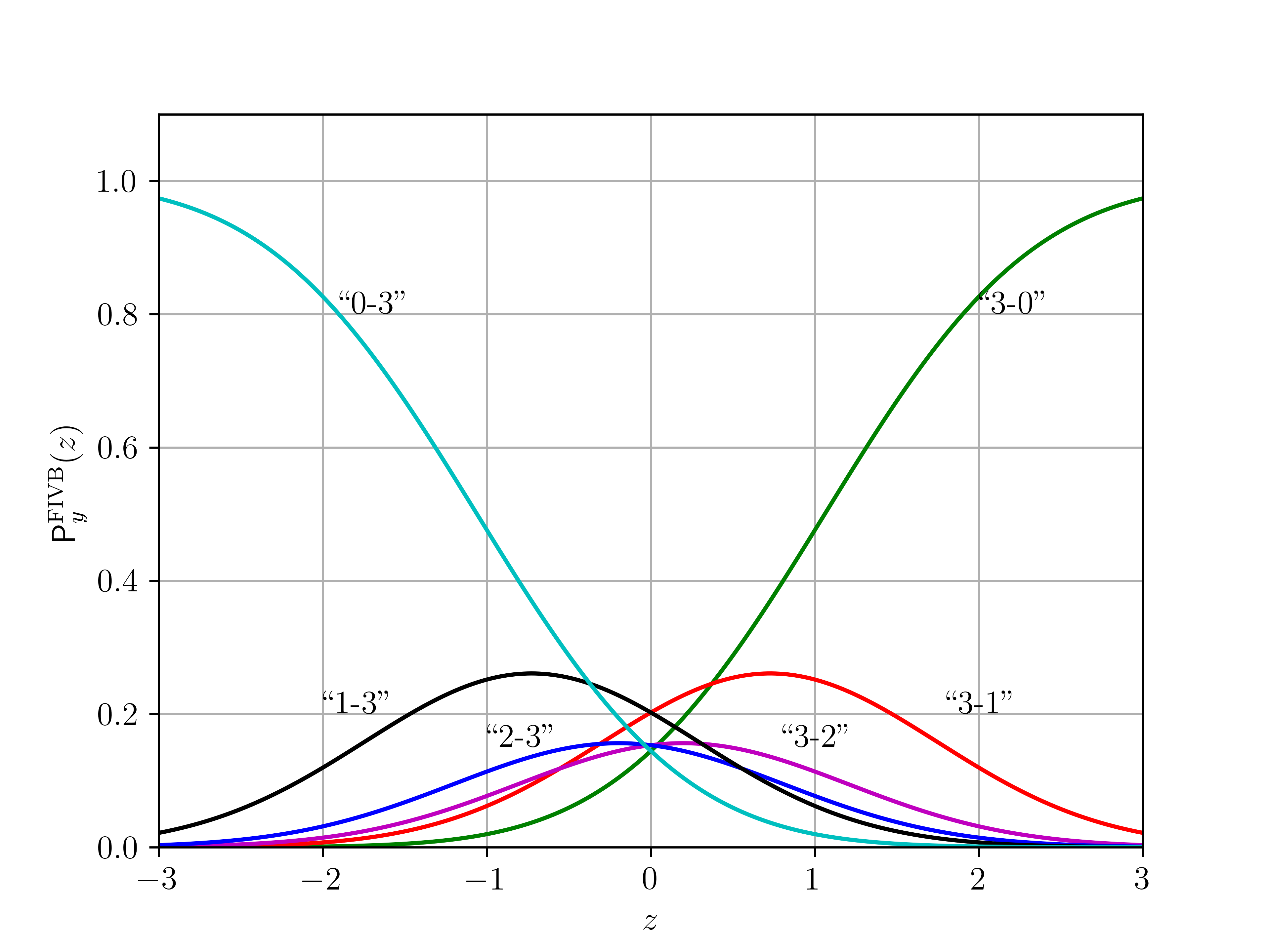
Figure 1: Functions $\mathsf{P}^{{\textnormal{FIVB}}}_{y}(z)$ in the FIVB rating algorithm, where $y=0$ corresponds to the result “3-0”, $y=1$ to “3-1”, etc.

With the model defined, the FIVB ranking algorithm estimates the skills as follows,(FIVB, 2024):

$$\boldsymbol{\theta}_{t+1} =\boldsymbol{\theta}_{t}-\mu s\xi_{v_{t}}\boldsymbol{x}_{t}g^{{\textnormal{FIVB}}}_{y_{t}}(z_{t}/s),$$ (25)

$$g^{\textnormal{FIVB}}_{y}(z) =\check{r}(z)-r^{\textnormal{FIVB}}_{y},$$ (26)

where the adaptation step is $\mu=0.01$, the scale is $s=125$, the weights $\xi_{v}$ are defined in Table 1, and $r^{\textnormal{FIVB}}_{y}$ is the numerical score assigned to the outcome $y$, see Table 2. It may be surprising because, as we emphasized previously, ordinal outcomes have no numerical value. This is still true: in fact, as we will see in Sec. 2.4, variables $r^{\textnormal{FIVB}}_{y}$ are merely auxiliary parameters defining the loss function $\ell^{{\textnormal{loss}}}_{y}(z)$, which is not the same as the log-score (6).

The probabilistic model (21) is used to calculate the expected value of $r^{\textnormal{FIVB}}_{Y}$ (for a given $z$):

$$\check{r}(z) =\mathds{E}_{Y|z}[r^{\textnormal{FIVB}}_{Y}]=\sum_{y\in\mathcal{Y}}r^{\textnormal{FIVB}}_{y}\mathsf{P}^{{\textnormal{FIVB}}}_{y}(z)$$ (27)

$$=\sum_{y=0}^{L-2}(r^{\textnormal{FIVB}}_{y}-r^{\textnormal{FIVB}}_{y+1})\Phi(z+c^{{\textnormal{FIVB}}}_{y})+r^{\textnormal{FIVB}}_{L-1}.$$ (28)

$v$	$\xi_{v}$	Description
$0$	$1.00$	Official events of Continental Confederations
$1$	$1.75$	Confederations’ Championship qualifying
$2$	$2.00$	FIVB Challenger Cup
$3$	$3.50$	Olympic Games qualifying,
		Confederations’ Championship
$4$	$4.00$	FIVB Nations League
$5$	$4.50$	FIVB World Championship
$6$	$5.00$	Olympic Games

Table 1: The weighting coefficients adopted from the FIVB ranking. Note that we normalize $\xi_{v}$ by using $\xi_{v}=1.0$.

$y$	“3-0”	“3-1”	“3-2”	“2-3”	“1-3”	“0-3”
$r^{\textnormal{FIVB}}_{y}$	2.0	1.5	1.0	-1.0	-1.5	-2.0

Table 2: Numerical values $r^{\textnormal{FIVB}}_{y}$ assigned to the outcomes $y$ in the FIVB rating algorithm.

The above presentation of the FIVB algorithm is meant to be compatible with the formulation in (17) but, of course, the official FIVB presentation in FIVB (2024) uses a different notation, as we explain in Appendix A. For example, instead of defining the step, the scale and the weights, their product $\mu s\xi_{v}$, used in (25) is defined.

The FIVB ranking has an additional rule which imposes a decrease of the rating by 50 points, $\theta_{m,t}\leftarrow\theta_{m,t}-50$, at the end of the year for each team $m$ that did not participate in any competition. The objective is to incentivize teams to play and discourage game avoidance, which might be a strategy used to preserve ranking points. But these are heuristics that cannot be easily put in the statistical framework, and thus we do not model them.

2.3 Data

To evaluate the FIVB ranking algorithm, we use the games played by the men’s national teams and published on the FIVB website FIVB (2024). We only consider the games since January 1, 2021, as, before that date, due to the Covid-19 pandemic, many games were eliminated and some had the weighting $\xi_{v}$ incompatible with the official description. The results were collected till the end of December 2023 (with no games after October 2023).

Since the FIVB website publishes the result of the game and the change in the value of skills, $\theta_{m,t+1}-\theta_{m,t}$, we can find the value of $\xi_{v}$ and infer the category of the game from Table 1. To establish the venue of the game, we relied on Wikipedia pages describing the international volleyball events, and matched them with the games from the FIVB website.

Moreover, we remove

• The games in which, the FIVB ranking displays increments with small absolute value $|\theta_{m,t+1}-\theta_{m,t}|\in\{0,0.01\}$. This may happen, e.g., when players could not obtain visas, and sometimes it is explained on the FIVB website (e.g., in the case of the Iranian team playing in the USA in 2023) but, in other cases, the non-standard values of $\xi$ are left unexplained. Since these games do not contribute to the change in the rating, excluding them from considerations is consistent with the spirit of the FIVB ranking.

• The forfeited games we could identify, even if the FIVB treats them as a “$3-0$” win: because the forfeited games do not reflect on the strength of the team, and thus we do no use them as information for rating.

Thus, we have a total of $M=102$ teams and $T=1151$ games. To characterize the results, we count games with result $y_{t}=y$, played on the neutral- and home-venues

$$k^{{\textnormal{ntr}}}_{y} =\frac{1}{2}\sum_{t=1}^{T}\big{(}\mathds{I}\big{[}{y_{t}=y,h_{t}=0}\big{]}+\mathds{I}\big{[}{y_{t}=L-1-y,h_{t}=0}\big{]}\big{)},$$ (29)

$$k^{{\textnormal{hfa}}}_{y} =\sum_{t=1}^{T}\mathds{I}\big{[}{y_{t}=y,h_{t}=1}\big{]}$$ (30)

and show them in Table 3.

Note that in neutral-venue games, there is no distinction between the home/away teams, so the number of results “$k-l$” (denoted as $y$) and “$l-k$” (denoted as $L-1-y$) should be equal: this is why we count all these results in (29). Although this produces a fractional value $k^{{\textnormal{ntr}}}_{y}$, this formalism simplifies the notation, and we guarantee that $k^{{\textnormal{ntr}}}_{y}=k^{{\textnormal{ntr}}}_{L-1-y}$.

$y$	“3-0”	“3-2”	“3-1”	“1-3”	“2-3”	“0-3”	Total
$k^{{\textnormal{ntr}}}_{y}$	203.5	117.5	59.5	59.5	117.5	203.5	761
$k^{{\textnormal{hfa}}}_{y}$	135	64	29	33	45	84	390

Table 3: Numbers of the FIVB games with outcomes $y\in\mathcal{Y}$, played on the neutral- and home- venues, and their totals.

2.4 Implicit loss function

Knowing the probabilistic model, we can derive the SG algorithm setting $\ell_{y}^{{\textnormal{loss}}}(z)=\ell_{y}(z)$, i.e., using the log-score as a loss function with

$$\ell_{y}(z) =-\log\big{(}\Phi(z+c_{y})-\Phi(z+c_{y-1})\big{)},$$ (31)

and finding the derivative of the latter

$$\dot{\ell}_{y}(z) =-\frac{\mathcal{N}(z+c_{y})-\mathcal{N}(z+c_{y-1})}{\Phi(z+c_{y})-\Phi(z+c_{y-1})}.$$ (32)

Quite obviously, plugging $\dot{\ell}_{y}(z)$ shown in (32), into the SG algorithm (17), does not produce the FIVB ranking (25). Thus, the FIVB ranking does not solve the ML or MAP problem.

To understand what problem it does solve, we note that, since the FIVB still has the structure of the SG optimization, we may treat the function $g^{{\textnormal{FIVB}}}_{y}(z)$ used by (25) as a derivative of an implicit (that is, not explicitly defined) loss function $\ell^{{\textnormal{FIVB}}}_{y}(z)$, i.e., $g^{{\textnormal{FIVB}}}_{y}(z)=\dot{\ell}^{{\textnormal{FIVB}}}_{y}(z)$, and, the latter can be unveiled through the integration of $g^{{\textnormal{FIVB}}}_{y}(z)$, i.e.,

$$\ell^{{\textnormal{FIVB}}}_{y}(z) =\int_{-\infty}^{z}g^{{\textnormal{FIVB}}}_{y}(u)\,\mathrm{d}u=\int_{-\infty}^{z}\big{[}\check{r}(u)-r^{\textnormal{FIVB}}_{y}\big{]}\,\mathrm{d}u,$$ (33)

$$=\sum_{l=0}^{L-2}(r^{{\textnormal{FIVB}}}_{l}-r^{{\textnormal{FIVB}}}_{l+1})\psi(z+c^{{\textnormal{FIVB}}}_{l})+(r^{\textnormal{FIVB}}_{L-1}-r^{\textnormal{FIVB}}_{y})z+{\textnormal{Const.}}$$ (34)

where (34) is obtained from (28) and

$$\psi(z) =\int_{-\infty}^{z}\Phi(u)\,\mathrm{d}u=\Phi(z)z+\mathcal{N}(z).$$ (35)

To understand why the FIVB ranking algorithm does not use directly the log-score (31), two issues with (32) should be considered.

The first is of numerical nature, because, for large $|z|$, both the numerator and the denominator in (32) tend to zero which requires a careful implementation.

The second problem is that (32) has a relatively complicated form without obvious interpretation. In that regard, (26) has the advantage: the skills are updated by the difference between the observed and expected numerical scores, and we note that this is also the usual interpretation of the well-known Elo algorithm Elo (2008).

We therefore conjecture that the FIVB rating algorithm was designed to be simple and understandable. The potential drawback is the sub-optimality of the rating results, which we will evaluate in this work.

Convergence

A minor point is to obtain a guarantee that, for a sufficiently small $\mu$, the FIVB algorithm (25) converges, for which we need the following:

Lemma 1.

The implicit loss function, $\ell^{{\textnormal{FIVB}}}_{y}(z)$ is convex in $z$.
Proof:
The second derivative of the implicit loss $\ell^{{\textnormal{FIVB}}}_{y}(z)$ is positive if the first derivative $g^{{\textnormal{FIVB}}}_{y}(z)=\check{r}(z)-r^{\textnormal{FIVB}}_{y}$ increases monotonically in $z$. The latter holds because (28) is monotonically increasing if $r^{\textnormal{FIVB}}_{y+1}<r^{\textnormal{FIVB}}_{y}$, which is true from Table 2.

We note that condition $r^{\textnormal{FIVB}}_{y+1}<r^{\textnormal{FIVB}}_{y}$ is sufficient but not necessary, i.e., it can be violated, and yet we can still obtain a convex function $\ell^{{\textnormal{FIVB}}}_{y}(z)$. The fact that this is possible only reinforces the idea that numerical scores are auxiliary parameters and should not be thought of as a value of the game outcome (because the latter, simply, do not exist).

3 Model identification

In this part of the work, we assume that

• The probabilistic model (21) is predefined, and we need to define the thresholds $\boldsymbol{c}$ and, eventually, the HFA coefficient $\eta$.

• The loss function is defined via $\ell^{{\textnormal{FIVB}}}_{y}(z)$ in (34), and we need to define the suitable numerical scores $\boldsymbol{r}=[r_{0},\ldots,r_{L-1}]$ which are attributed to the outcomes, and

• The weights $\boldsymbol{\xi}$ are used in the algorithm via (19), and we want to assess their usefulness.

In order to assess and/or optimize the parameters of the model, we need a well-defined criterion.

3.1 Model identification via cross-validation

The inference (12) may be done if we define (the form of) the loss and the regularization functions, as well as, if we find their parameters $\boldsymbol{p}$ (also called hyper-parameters, in the machine learning language) which affect all the functions describing the models, i.e., we can write $\ell^{{\textnormal{loss}}}(z)\equiv\ell^{{\textnormal{loss}}}_{y}(z;\boldsymbol{p})$, $\ell_{y}(z)\equiv\ell_{y}(z;\boldsymbol{p})$ and $\rho(\boldsymbol{\theta})\equiv\rho(\boldsymbol{\theta};\boldsymbol{p})$.

A well-known approach to finding the hyper-parameters, particularly suitable for relatively small data sets, relies on cross-validation, where we split the data into multiple training and validation sets (Barber, 2012, Ch. 13.2.2), and we verify how well the results (12) match the validation data using a metric $\ell^{{\textnormal{val}}}_{y}(\boldsymbol{x}^{\mathsf{T}}\hat{\boldsymbol{\theta}})$.

If we know the model (1), and especially if we use the log-score as the loss function, i.e., in $\ell^{{\textnormal{loss}}}_{y}(z)=\ell_{y}(z)$, the validation metric used in practice is also the log-score

$$\ell^{{\textnormal{val}}}_{y}(z) =\ell_{y}(z);$$ (37)

this is the metric we use here as well.

We will use the leave-one-out (LOO) cross-validation, where the validation sets contain only one sample and thus, we can consider all possible $T$ validation/testing splits, (Hastie et al., 2009, Ch. 2.9)

$$\hat{\boldsymbol{p}} =\mathop{\mathrm{argmin}}_{\boldsymbol{p}}U(\boldsymbol{p})$$ (38)

$$U(\boldsymbol{p}) =\frac{1}{T}\sum_{t=1}^{T}\ell_{y_{t}}^{{\textnormal{val}}}(\hat{z}_{t,\backslash{t}};\boldsymbol{p})$$ (39)

$$\hat{z}_{t,\backslash{t}} =\boldsymbol{x}^{\mathsf{T}}_{t}\hat{\boldsymbol{\theta}}_{\backslash{t}}$$ (40)

$$\hat{\boldsymbol{\theta}}_{\backslash{\tau}} =\mathop{\mathrm{argmin}}_{\boldsymbol{\theta}}\big{[}J(\boldsymbol{\theta})-\ell^{{\textnormal{loss}}}_{y_{\tau}}(\boldsymbol{x}^{\mathsf{T}}_{\tau}\boldsymbol{\theta};\boldsymbol{p})\big{]}.$$ (41)

We note that (39) can be transformed as follows:

$$V(\boldsymbol{p})=\mathrm{e}^{-U(\boldsymbol{p})}=\Big{[}\prod_{t=1}^{T}\mathsf{P}_{y_{t}}(\hat{z}_{t,\backslash{t}};\boldsymbol{p}))\Big{]}^{\frac{1}{T}},$$ (42)

which is the geometric mean of the probabilities of observing $Y_{t}=y_{t}$, calculated from $\hat{\boldsymbol{\theta}}_{\backslash{t}}$. Thus, $V(\boldsymbol{p})$ is potentially easier to interpret than $U(\boldsymbol{p})$; and, with linearization, for small $U(\boldsymbol{p})$, e.g., $U(\boldsymbol{p})<0.1$, we have $V(\boldsymbol{p})\approx 1-U(\boldsymbol{p})$.

Although using the LOO strategy eliminates the ambiguity of how the validation sets are selected (we test all, $T$ possible testing/validations splits), solving $T$ times the optimization problem (41) becomes computationally demanding.

Thus, instead, we use the approximate leave-one-out (ALO) approach (Beirami et al., 2017, Rad and Maleki, 2020, Burn, 2020): we solve (12) once to find $\hat{\boldsymbol{\theta}}\equiv\hat{\boldsymbol{\theta}}(\boldsymbol{p})$ (this is where most of the computational complexity lies), and make a quadratic approximation of the function $J(\boldsymbol{\theta})$ around $\hat{\boldsymbol{\theta}}$, which allows us to find the closed-form approximation of (40) as follows:

$$\hat{z}_{t,\backslash{t}} \approx\hat{z}_{t}+\frac{\dot{\ell}^{{\textnormal{loss}}}_{y_{t}}(\hat{z}_{t};\boldsymbol{p})a_{t}}{1-\ddot{\ell}^{{\textnormal{loss}}}_{y_{t}}(\hat{z}_{t};\boldsymbol{p})a_{t}},$$ (43)

where $a_{t}=\boldsymbol{x}^{\mathsf{T}}_{t}\hat{{\textnormal{{H}}}}^{-1}\boldsymbol{x}_{t}$, $\hat{{\textnormal{{H}}}}=\nabla^{2}_{\boldsymbol{\theta}}J(\boldsymbol{\theta})|_{\boldsymbol{\theta}=\hat{\boldsymbol{\theta}}}$ is the Hessian of the function $J(\boldsymbol{\theta})$ under minimization in (12), $\ddot{\ell}^{{\textnormal{loss}}}_{y}(z;\boldsymbol{p})=\frac{\,\mathrm{d}}{\,\mathrm{d}z}\dot{\ell}^{{\textnormal{loss}}}_{y}(z;\boldsymbol{p})$, and $\hat{z}_{t}=\boldsymbol{x}^{\mathsf{T}}_{t}\hat{\boldsymbol{\theta}}(\boldsymbol{p})$. Details of the derivation can be found in (Burn, 2020, Sec. 3) or (Szczecinski and Roatis, 2022, Appendix. 2).

We may use, of course, $\ell_{y_{t},v_{t}}^{{\textnormal{loss}}}(z_{t};\boldsymbol{p})$ or $\ell_{y_{t},h_{t}}^{{\textnormal{loss}}}(z_{t};\boldsymbol{p})$ defined in (18) or (19), and then the first/second derivatives used in (43) should be calculated as

$$\dot{\ell}_{y_{t},v_{t}}^{{\textnormal{loss}}}(z_{t};\boldsymbol{p}) =\xi_{v_{t}}\dot{\ell}_{y_{t}}^{{\textnormal{loss}}}(z_{t};\boldsymbol{p}),$$ (44)

$$\ddot{\ell}_{y_{t},v_{t}}^{{\textnormal{loss}}}(z_{t};\boldsymbol{p}) =\xi_{v_{t}}\ddot{\ell}_{y_{t}}^{{\textnormal{loss}}}(z_{t};\boldsymbol{p}),$$ (45)

$$\dot{\ell}_{y_{t},h_{t}}^{{\textnormal{loss}}}(z_{t};\boldsymbol{p}) =\dot{\ell}_{y_{t}}^{{\textnormal{loss}}}(z_{t}+h_{t}\eta;\boldsymbol{p}),$$ (46)

$$\ddot{\ell}_{y_{t},h_{t}}^{{\textnormal{loss}}}(z_{t};\boldsymbol{p}) =\ddot{\ell}_{y_{t}}^{{\textnormal{loss}}}(z_{t}+h_{t}\eta;\boldsymbol{p}).$$ (47)

If we predefine candidate hyperparameters in the set $\mathcal{P}=\{\boldsymbol{p}_{{\textnormal{a}}},\boldsymbol{p}_{{\textnormal{b}}},\boldsymbol{p}_{{\textnormal{c}}},\ldots\}$, e.g., using those specified in the existing ranking, or modifying them using a particular insight into the ranking problem, the optimization is simple:

$$\hat{\boldsymbol{p}}=\mathop{\mathrm{argmin}}_{\boldsymbol{p}\in\mathcal{P}}U(\boldsymbol{p})$$ (48)

and is essentially done by comparing the value of $U(\boldsymbol{p})$ for all candidates in $\mathcal{P}$.

On the other hand, optimizing the value of the hyperparameters $\boldsymbol{p}$ as suggested by (38) is more difficult but can be done with appropriate numerical tools, as we explain in Appendix B.

Empirical entropy as a comparison baseline

Model identification results can be compared to a simple baseline, where we assume that the prediction of the game result $Y_{t}$ is based on the empirical frequency of the results observed in all other games, i.e.,

$$\tilde{\ell}^{{\textnormal{val}}}_{y_{t}}=-\log\frac{k_{y_{t}}-1}{T-1},$$ (49)

where

$$k_{l}=k^{{\textnormal{ntr}}}_{l}+k^{{\textnormal{hfa}}}_{l},$$ (50)

is the venue-independent game count.

Then, the frequency-based performance baseline (39) is found as

$$\tilde{U} =-\frac{1}{T}\sum_{t=1}^{T}\log\frac{k_{y_{t}}-1}{T-1}$$ (51)

$$=-\sum_{l=0}^{L-1}\frac{k_{l}}{T}\log\frac{k_{l}-1}{T-1}=H(\boldsymbol{q},T)$$ (52)

where $\boldsymbol{q}=[q_{0},\ldots,q_{L-1}]$, $q_{l}=k_{l}/T$ is the empirical frequency of events $Y_{t}=l$, and

$$H(\boldsymbol{q},T)=-\sum_{l=0}^{L-1}q_{l}\log\frac{q_{l}-1/T}{1-1/T};$$ (53)

for large $T$, (53) tends to the entropy $H(\boldsymbol{q})$ of the source which generates the outcomes $Y_{t}$ with probabilities defined in the vector $\boldsymbol{q}$.

If we take into account the HFA, (51) becomes

$$\tilde{U} =\frac{1}{T}\Big{[}T^{{\textnormal{ntr}}}\tilde{U}^{{\textnormal{ntr}}}+T^{{\textnormal{hfa}}}\tilde{U}^{{\textnormal{hfa}}}\Big{]}$$ (54)

$$\tilde{U}^{{\textnormal{ntr}}} =H(\boldsymbol{q}^{{\textnormal{ntr}}},T^{{\textnormal{ntr}}})$$ (55)

$$\tilde{U}^{{\textnormal{ntr}}} =H(\boldsymbol{q}^{{\textnormal{hfa}}},T^{{\textnormal{hfa}}})$$ (56)

where, $T^{{\textnormal{ntr}}}=\sum_{l=0}^{L-1}k^{{\textnormal{ntr}}}_{l}$, $T^{{\textnormal{hfa}}}=\sum_{l=0}^{L-1}k^{{\textnormal{hfa}}}_{l}$, $\boldsymbol{q}^{{\textnormal{ntr}}}=[k^{{\textnormal{ntr}}}_{0}/T^{{\textnormal{ntr}}},\ldots,k^{{\textnormal{ntr}}}_{L-1}/T^{{\textnormal{ntr}}}]$, and $\boldsymbol{q}^{{\textnormal{hfa}}}=[k^{{\textnormal{hfa}}}_{0}/T^{{\textnormal{hfa}}},\ldots,k^{{\textnormal{hfa}}}_{L-1}/T^{{\textnormal{hfa}}}]$.

These entropy-like metrics, shown in Table 4, are performance upper bounds in the sense that any well-designed rating strategy, which uses $\hat{\boldsymbol{\theta}}_{\backslash{t}}$ as a basis for predicting the outcomes, should provide the cross-validation metric $U(\boldsymbol{p})$ that is smaller than the value $\tilde{U}$ shown in Table 4a, and larger than the corresponding average probabilities $\tilde{V}$ shown in Table 4b.

$\tilde{U}$	$\tilde{U}^{{\textnormal{ntr}}}$	$\tilde{U}^{{\textnormal{hfa}}}$
1.68	1.69	1.66

a)
$\tilde{V}$ $\tilde{V}^{{\textnormal{ntr}}}$ $\tilde{V}^{{\textnormal{hfa}}}$ 0.19 0.18 0.19
b)

Table 4: Empirical entropy defined in (54), (55), and (56), calculated for the games FIVB, as well as their transformation via (42).

Similarly, the reference metrics $\tilde{U}^{{\textnormal{ntr}}}$ and $\tilde{U}^{{\textnormal{hfa}}}$ should be treated as trivial upper bounds on the cross-validation results conditioned on the game venue

$$U^{{\textnormal{ntr}}}(\boldsymbol{p}) =\frac{1}{T^{{\textnormal{ntr}}}}\sum_{\begin{subarray}{c}t=1\\ h_{t}=0\end{subarray}}^{T}\ell^{{\textnormal{val}}}(\hat{z}_{t,\backslash{t}};\boldsymbol{p})$$ (57)

$$U^{{\textnormal{hfa}}}(\boldsymbol{p}) =\frac{1}{T^{{\textnormal{hfa}}}}\sum_{\begin{subarray}{c}t=1\\ h_{t}=1\end{subarray}}^{T}\ell^{{\textnormal{val}}}(\hat{z}_{t,\backslash{t}};\boldsymbol{p}),$$ (58)

Of course, we can recover (39) as $U(\boldsymbol{p})=[T^{{\textnormal{ntr}}}U^{{\textnormal{ntr}}}(\boldsymbol{p})+T^{{\textnormal{hfa}}}U^{{\textnormal{hfa}}}(\boldsymbol{p})]/T$, see also (54).

3.2 Finding thresholds $c$ and HFA parameter $\eta$

To assess the role of the thresholds $\boldsymbol{c}^{{\textnormal{FIVB}}}$ used in the CL model (21) and of the HFA parameter $\eta$, we start with $\ell^{{\textnormal{loss}}}_{y}(z)=\ell_{y}(z)$ and consider four cases:

1. We use $\boldsymbol{c}=\boldsymbol{c}^{{\textnormal{FIVB}}}$ given by (23) and $\eta=0$; in other words, no optimization is performed.

2. We find $\hat{\boldsymbol{c}}$ by optimizing $U(\boldsymbol{p})$ in (38) but we set $\eta=0$, i.e.,

   $$\hat{\boldsymbol{c}}=\mathop{\mathrm{argmin}}_{\boldsymbol{c},\eta=0}U(\boldsymbol{c}).$$ (59)

3. We use $\boldsymbol{c}^{{\textnormal{FIVB}}}$ and optimize the HFA parameter, i.e., use

   $$\hat{\eta}=\mathop{\mathrm{argmin}}_{\eta,\boldsymbol{c}=\boldsymbol{c}^{{\textnormal{FIVB}}}}U(\eta);$$ (60)

4. We find both $\hat{\boldsymbol{c}}$ and $\hat{\eta}$ through optimization,

   $$\hat{\boldsymbol{c}},\hat{\eta}=\mathop{\mathrm{argmin}}_{\boldsymbol{c},\eta}U(\boldsymbol{c},\eta),$$ (61)

   and they are shown in Fig. 2.

In the above, we slightly abuse the notation and write e.g., $U(\boldsymbol{c})$ to indicate that we optimize only the parameter $\boldsymbol{c}$ and all other hyperparameters in $\boldsymbol{p}$ are kept constant (as we also explicitly indicate, when relevant, under the $\mathop{\mathrm{argmin}}$ operator); similarly, the notation $U(\boldsymbol{c},\eta)$ means that both $\boldsymbol{c}$ and $\eta$ are optimized.

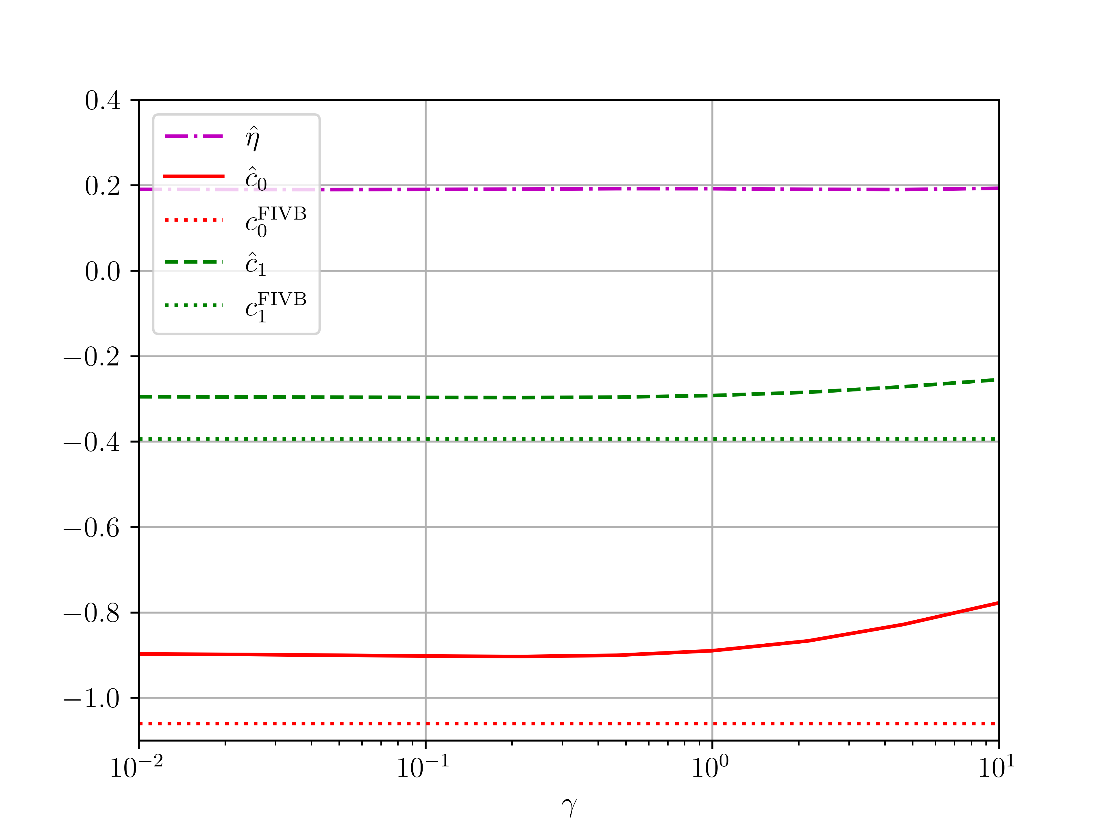
Figure 2: Results of optimization in (61): thresholds $\hat{c}_{0}$, $\hat{c}_{1}$ and the HFA $\hat{\eta}$. The horizontal dotted lines are drawn for the values $c^{{\textnormal{FIVB}}}_{0}=-1.06$ and $c^{{\textnormal{FIVB}}}_{1}=-0.394$ used by the FIVB ranking, see (23).

We show, in Fig. 3, cross-validation results $U^{{\textnormal{ntr}}}(\boldsymbol{p})$ and $U^{{\textnormal{hfa}}}(\boldsymbol{p})$ defined in (57) and (58) as functions of the regularization parameter $\gamma$, where $\boldsymbol{p}$ contains all parameters, including $\gamma$ and others that are optimized according to the cases we explain above. The right-hand axis in Fig. 3 shows the metric $V(\boldsymbol{p})$ as a transformation of $U(\boldsymbol{p})$ through (42).

Figure 3: Validation metrics $U^{{\textnormal{ntr}}}$ (hollow markers) and $U^{{\textnormal{hfa}}}$ (colored markers) given by (57)-(58) shown as a function of $\gamma$ using the loss function $\ell_{y}(z)$ defined in (6).

Main observations

• The FIVB thresholds $\boldsymbol{c}^{{\textnormal{FIVB}}}$ are close, but not identical to, those obtained via optimization. This discrepancy should be attributed to the difference in the data sets from which the thresholds were inferred, but also due to the procedure described by the FIVB ranking, which defined $\boldsymbol{c}$ from the games of the “teams with similar skills”.

  In our approach, we used all the games, which may explain some improvement in the average validation metric $U(\boldsymbol{p})$.

• The decomposition into the games played on the neutral and home venues indicates that, by including the HFA into the model via $\eta>0$, we can improve the prediction for the home games, and, rather unsurprisingly, this modification has practically no impact on the neutral-venue games.

• Attention should be paid to the metric $V(\boldsymbol{p})$ shown in the right axis, where we see that the improvements are at the order of fraction of a percent. For example, the most significant improvement appears for home-games, where, incorporation of $\eta>0$ and optimization of the thresholds, improve the results, by $\sim 1\%$; i.e., from $V\approx 25.8\%$ to $V\approx 26.8\%$. This can be compared to the performance of the empirical entropy shown in Table 4, which is notably worse.

3.3 Finding numerical score $r$

To discuss the role of the numerical scores $\boldsymbol{r}$ used in the FIVB algorithm, we will first, in Sec. 3.3.1, analyze the implicit loss functions used by the algorithm while a purely numerical analysis / optimization is carried out in Sec. 3.3.2.

3.3.1 From thresholds to numerical scores

We show, in Fig. 4, the logarithmic loss functions $\ell_{y}(z)$, as well as, the scaled and vertically-shifted versions of the implicit loss functions $a\ell^{{\textnormal{FIVB}}}_{y}(z;\boldsymbol{r})+b_{y}$, where we find $a$ by matching the first derivatives of the loss function $\ell_{0}(z_{{\textnormal{o}}})$ for $z=z_{{\textnormal{o}}}=0$

$$\dot{\ell}_{0}(z_{{\textnormal{o}}}) =ag^{{\textnormal{FIVB}}}_{0}(z_{{\textnormal{o}}};\boldsymbol{r}),$$ (62)

which, from $g^{{\textnormal{FIVB}}}_{y}(z_{{\textnormal{o}}};\boldsymbol{r})=\check{r}(z_{{\textnormal{o}}})-r_{y}=-r_{y}$, yields

$$a =-\frac{\dot{\ell}_{0}(z_{{\textnormal{o}}})}{r_{0}}.$$ (63)

Similarly, the shifts $b_{y}$ are calculated to match the values of the loss functions at $z_{{\textnormal{o}}}$, i.e., to satisfy $\ell_{y}(z_{{\textnormal{o}}})=a\ell^{{\textnormal{FIVB}}}_{y}(z_{{\textnormal{o}}};\boldsymbol{r})+b_{y}$. This means that $b_{y}=\ell_{y}(z_{{\textnormal{o}}})-a\ell^{{\textnormal{FIVB}}}_{y}(z_{{\textnormal{o}}};\boldsymbol{r})$.

This scaling/shifting transformation is irrelevant from the optimization point of view, but allows us to visually appreciate the difference between the loss functions in the vicinity of the target value $z_{{\textnormal{o}}}=0$. Note that assuming that $z_{t}$ will be mostly observed close to $z_{{\textnormal{o}}}$ is compatible with $z$ being a zero-mean Gaussian variable, which is the modeling assumption we used in Sec. 3.2.

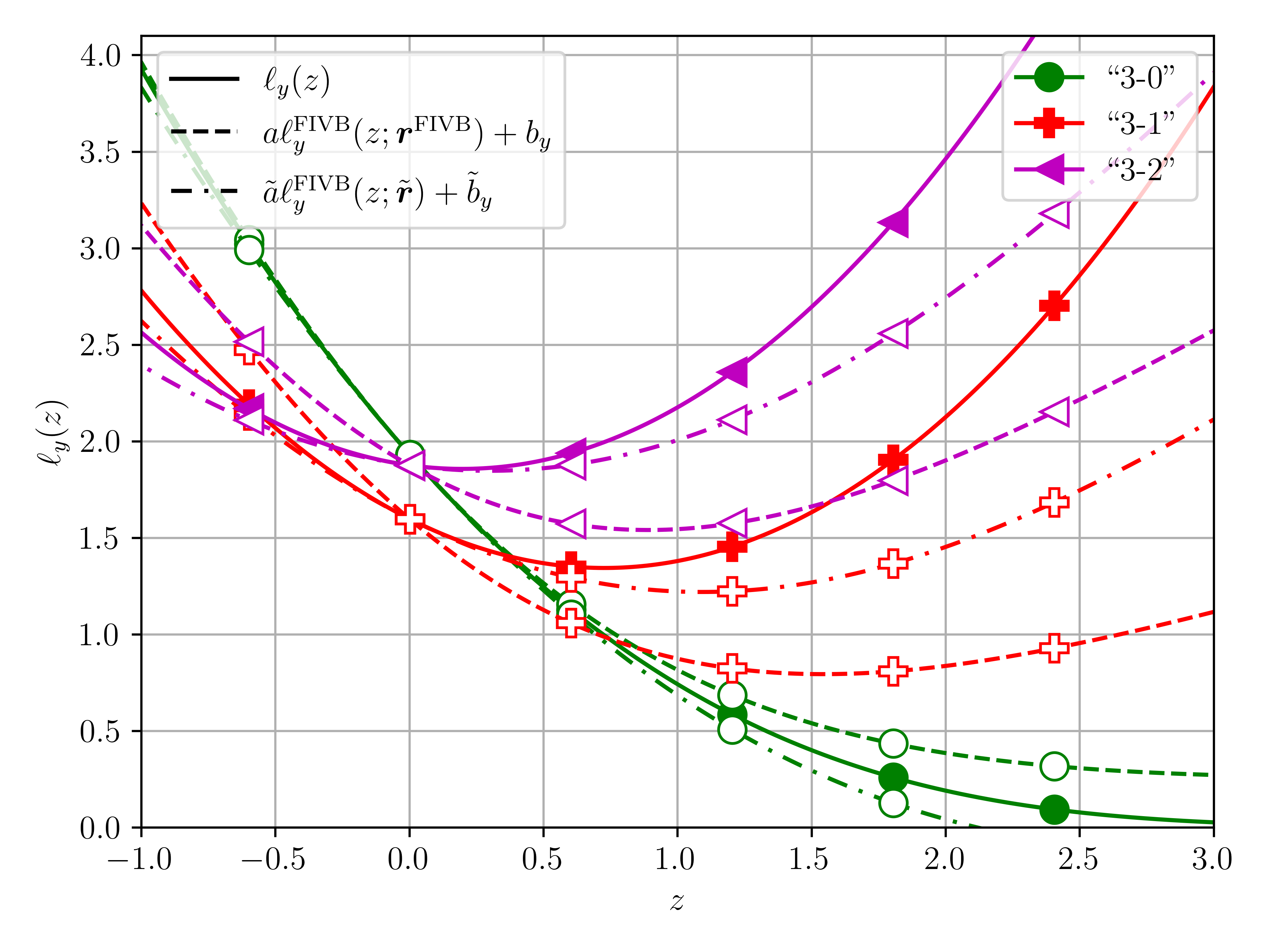
Figure 4: Loss functions: log-score $\ell_{y}(z)$ (solid line) and rescaled/shifted implicit loss function $a\ell^{{\textnormal{FIVB}}}_{y}(z;\boldsymbol{r})+b_{y}$ (dashed line) for $y=0,1,2$ corresponding, respectively, to the outcomes “3-0”, “3-1”, and “3-2”.

Indeed, Fig. 4 indicates that an almost perfect match is obtained for $\ell_{0}(z)$, i.e., the logarithmic loss is practically indistinguishable from the scaled/shifted implicit loss. However, the loss functions are not matched for $y=1,2$, and we want to find the numerical score $\tilde{\boldsymbol{r}}=[\tilde{r}_{0},\ldots,\tilde{r}_{L-1}]$, which satisfies a generalized version of (62), i.e., we want the latter to hold for all $y\in\mathcal{Y}$, that is

$$\dot{\ell}_{y}(z_{{\textnormal{o}}})=ag_{y}^{{\textnormal{FIVB}}}(z_{{\textnormal{o}}};\tilde{\boldsymbol{r}}),\quad y\in\mathcal{Y}.$$ (64)

Since $\dot{\ell}_{y}(z_{0})=g_{y}^{{\textnormal{FIVB}}}(z_{{\textnormal{o}}};\tilde{\boldsymbol{r}})=-\tilde{r}_{y}$, (64) is solved by

$$\tilde{r}_{y}\equiv\tilde{r}_{y}(\boldsymbol{c}) =-\tilde{r}_{0}\frac{\dot{\ell}_{y}(z_{{\textnormal{o}}})}{\dot{\ell}_{0}(z_{{\textnormal{o}}})}=\tilde{r}_{0}\frac{\Phi(c_{0})\big{(}\mathcal{N}(c_{y})-\mathcal{N}(c_{y-1})\big{)}}{\mathcal{N}(c_{0})\big{(}\Phi(c_{y})-\Phi(c_{y-1})\big{)}},\quad y\in\mathcal{Y},$$ (65)

where we used (32) and (63); the notation $\tilde{r}_{y}(\boldsymbol{c})$ emphasizes the dependence of $\tilde{\boldsymbol{r}}$ on the thresholds $\boldsymbol{c}$ which define the CL model. Note also that $\tilde{r}_{y}$ is not uniquely defined, as $\tilde{r}_{0}$ can be arbitrarily fixed, and, for comparison with the FIVB ranking, we set $\tilde{r}_{0}\equiv r^{{\textnormal{FIVB}}}_{0}=2.0$.

Using $\boldsymbol{c}=\boldsymbol{c}^{{\textnormal{FIVB}}}$ in (65) yields

$$\tilde{r}_{0} =-\tilde{r}_{5}\equiv 2.0,$$ (66)

$$\tilde{r}_{1}(\boldsymbol{c}^{{\textnormal{FIVB}}}) =-\tilde{r}_{4}(\boldsymbol{c}^{{\textnormal{FIVB}}})=0.89,$$ (67)

$$\tilde{r}_{2}(\boldsymbol{c}^{{\textnormal{FIVB}}}) =-\tilde{r}_{3}(\boldsymbol{c}^{{\textnormal{FIVB}}})=0.25.$$ (68)

These values are rather different from those shown in Table 2 and, more importantly, when we use them to calculate the implicit loss functions $\ell^{{\textnormal{FIVB}}}_{y}(z;\tilde{\boldsymbol{r}}),y=0,1,2$ (shown, scaled with $\tilde{a}$ and shifted with $\tilde{b}$, in Fig. 4 with dashed-dotted lines), the latter are indistinguishable from $\ell_{y}(z)$ in the vicinity of $z_{{\textnormal{o}}}=0$.

3.3.2 Numerical optimization

Instead of the analytical approach, shown in the previous section, the numerical optimization of $\boldsymbol{r}$, takes into account the actual outcomes of the games.

To analyze the optimality of $\boldsymbol{r}^{{\textnormal{FIVB}}}$, the loss function $\ell^{{\textnormal{loss}}}_{y}(z)$ is set to $\ell^{{\textnormal{FIVB}}}_{y}(z)$, and we consider the following cases:

1. We use $\boldsymbol{c}^{\textnormal{FIVB}}$ and $\boldsymbol{r}^{\textnormal{FIVB}}$ specified by the FIVB ranking, and given, respectively, in (23) and Table 2, and we set $\eta=0$. This is the reference, currently used by the FIVB.

2. We optimize $\boldsymbol{r}$, $\eta$ for a given $\boldsymbol{c}$

   $$\hat{\boldsymbol{r}}(\boldsymbol{c}),\hat{\eta}(\boldsymbol{c})=\mathop{\mathrm{argmin}}_{\boldsymbol{r},\eta}U(\boldsymbol{r},\eta,\boldsymbol{c},\boldsymbol{p}_{\backslash\{\boldsymbol{r},\eta,\boldsymbol{c}\}}),$$ (69)

   where we consider $\boldsymbol{c}=\boldsymbol{c}^{\textnormal{FIVB}}$ and $\boldsymbol{c}=\hat{\boldsymbol{c}}$, with the latter obtained via (61).

3. We calculate the numerical score $\tilde{\boldsymbol{r}}=\tilde{\boldsymbol{r}}\big{(}\boldsymbol{c}\big{)}$ using the formula shown in (65), and set $\eta=0.2$ (which is a rounded value of $\hat{\eta}$ obtained through optimization; see Fig. 2). As before, this is done for $\boldsymbol{c}=\boldsymbol{c}^{\textnormal{FIVB}}$ and $\boldsymbol{c}=\hat{\boldsymbol{c}}$.

Figure 5: Validation metrics $U^{{\textnormal{ntr}}}$ (hollow markers) and $U^{{\textnormal{hfa}}}$ (colored markers) given by (57)-(58) shown as a function of $\gamma$ for the loss function $\ell^{{\textnormal{loss}}}_{y}(z)=\ell^{{\textnormal{FIVB}}}_{y}(z)$ defined in (34) using parameters which may be: predefined ($\boldsymbol{r}^{{\textnormal{FIVB}}}$), analyticaly calculated ($\tilde{\boldsymbol{r}}\big{(}\boldsymbol{c}^{{\textnormal{FIVB}}}\big{)}$), or, numerically optimized ($\hat{\boldsymbol{r}}$).

The ALO metrics are shown in Fig. 5, where we observe:

• The ALO metric obtained with optimized numerical scores $\hat{\boldsymbol{r}}$ and with the calculated ones $\tilde{\boldsymbol{r}}(\boldsymbol{c})$ are practically identical, which supports our analysis in Sec. 3.3.1.

• By comparing the results from Fig. 5 with those shown in Fig. 4 we see that, using the implicit FIVB loss functions, $\ell^{{\textnormal{FIVB}}}_{y}(z)$, and provided the numerical scores $\boldsymbol{r}$ are adequately set (i.e., optimized via (69) or calculated via (65)), a negligible loss of performance is incurred when comparing to the log-score $\ell_{y}(z)$. This justifies the choice made in the FIVB ranking which avoids the exact, but complicated derivative of the loss function shown in (32).

• The numerical scores $\boldsymbol{r}^{{\textnormal{FIVB}}}$ currently used in the FIVB ranking, lead to the observable performance loss.

The numerical score $\boldsymbol{r}^{{\textnormal{FIVB}}}$ used currently in the ranking is compared, in Fig. 6, to $\hat{\boldsymbol{r}}(\boldsymbol{c}^{{\textnormal{FIVB}}})$ which is obtained by optimization (69) and to $\tilde{\boldsymbol{r}}(\boldsymbol{c}^{{\textnormal{FIVB}}})$ – calculated from (65); since $\boldsymbol{r}^{{\textnormal{FIVB}}}$ and $\tilde{\boldsymbol{r}}(\boldsymbol{c}^{{\textnormal{FIVB}}})$ do not depend on the regularization parameter $\gamma$, they are shown as horizontal lines. Also note that $r_{0}^{{\textnormal{FIVB}}}=\tilde{r}_{0}(\boldsymbol{c}^{{\textnormal{FIVB}}})=\hat{r}_{0}(\boldsymbol{c}^{{\textnormal{FIVB}}})=2$.

The optimized numerical scores $\hat{\boldsymbol{r}}$ change with $\gamma$, but have no incidence on the prediction capacity of the model, as shown already in Fig. 5. In fact, for $\gamma\approx 0.5$, which minimizes the total loss function, we get $\tilde{r}_{1}(\boldsymbol{c}^{{\textnormal{FIVB}}})\approx\hat{r}_{1}(\boldsymbol{c}^{{\textnormal{FIVB}}})$.

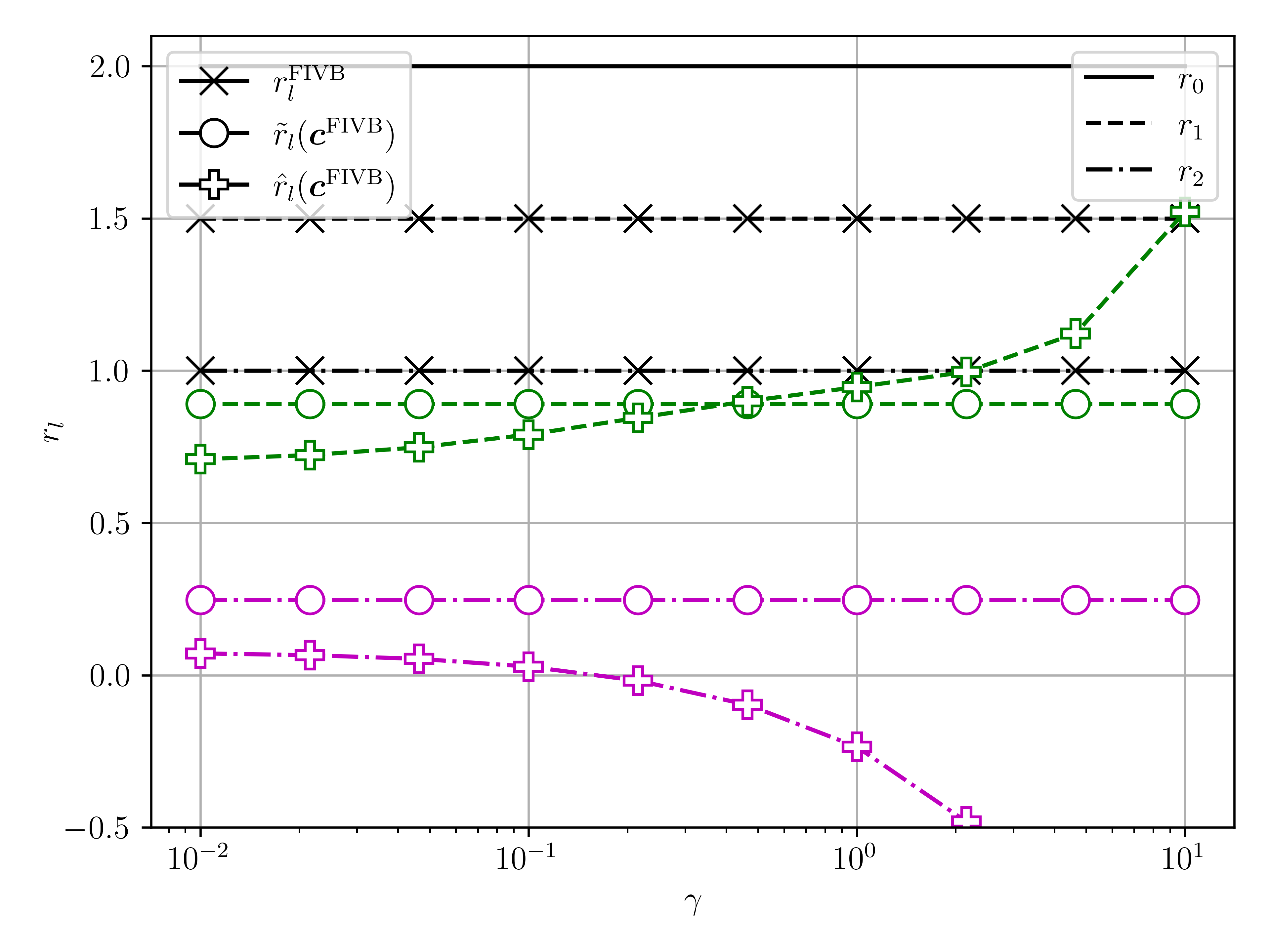
Figure 6: Numerical scores: $r_{l}^{{\textnormal{FIVB}}}$ given by the FIVB ranking, $\tilde{r}_{l}(\boldsymbol{c}^{{\textnormal{FIVB}}})$ calculated via (65), and $\hat{r}_{l}(\boldsymbol{c}^{{\textnormal{FIVB}}})$ optimized in (69).

On the other hand, $\hat{r}_{2}(\boldsymbol{c}^{{\textnormal{FIVB}}})$ becomes negative. For example, using the results for $\gamma\approx 0.5$ implies using,

$$\hat{r}_{0} =2.0,\quad\hat{r}_{1}\approx 0.9,\quad\hat{r}_{2}\approx-0.1,\quad\hat{r}_{3}\approx 0.1,\quad\hat{r}_{4}\approx-0.9,\quad\hat{r}_{4}=-2,$$ (70)

i.e., the numerical score does not decrease monotonically with the outcomes index, $y$.

This may appear surprising and counterintuitive, but only if we interpret the numerical score as related to the order of the outcomes. We should remember that ordinal variables do not have intrinsic numerical values, and numerical scores are parameters that allow us to adjust the form of the implicit loss function $\ell^{\text{FIVB}}_{y}(z)$. With such a perspective, the non-monotonic behavior of $r_{y}$ is allowed.

We also note that we always obtain more “conventional” (monotonic in $y$) behavior of $\tilde{r}_{y}(\boldsymbol{c})$. Since the optimized scores, $\hat{\boldsymbol{r}}$, and the calculated ones, $\tilde{\boldsymbol{r}}$, do not change the performance, it may be preferable to use the latter.

Immediate conclusion is that, the numerical score $\boldsymbol{r}^{{\textnormal{FIVB}}}$ is inadequately set in the current version of the FIVB ranking. However, it can be easily modified, e.g., using rounded values, $\tilde{r}_{1}=1.0$ and $\tilde{r}_{2}=0.25$.

Thus, it appears that the numerical scores $\boldsymbol{r}^{{\textnormal{FIVB}}}$ were not formally optimized — a conjecture supported by the fact that their origin is not explained in FIVB (2024).

We speculate that the numerical scores $\boldsymbol{r}$ are defined to be similar to the points in the volleyball leagues, where winning “$3-0$” grants $3$ points to the winner, winning “$3-1$” grants $2$ points, and winning “$3-2$” grants $1$ point. Multiplying these points by $2/3$, this scoring rule would be equivalent to granting $2.0$, $1.33$, and $0.66$ points – values somewhat similar to $r^{{\textnormal{FIVB}}}_{0}=2.0$, $r^{{\textnormal{FIVB}}}_{1}=1.5$, and $r^{{\textnormal{FIVB}}}_{2}=1.0$.

Regardless of the origin of $\boldsymbol{r}^{{\textnormal{FIVB}}}$, it is more sound to see the numerical score $\boldsymbol{r}$ as free parameters which allow us to make the implicit loss function $\ell^{{\textnormal{FIVB}}}_{y}(z;\boldsymbol{r})$ “behave” similarly to the optimal logarithmic loss $\ell_{y}(z)$.

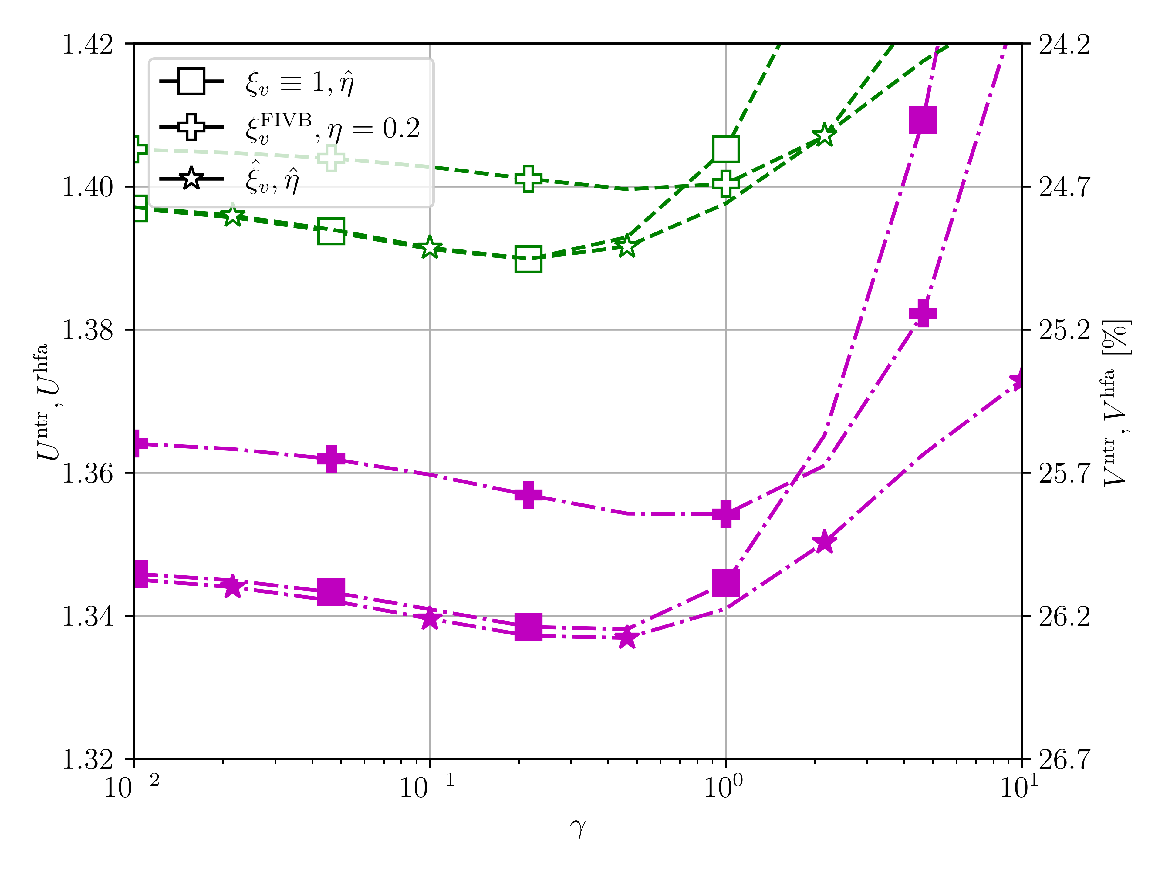
Figure 7: Validation metrics $U^{{\textnormal{ntr}}}$ (hollow markers) and $U^{{\textnormal{hfa}}}$ (colored markers) given by (57)-(58) shown as a function of $\gamma$ using the loss function $\ell_{y}(z)$ defined in (19) and different strategies of fixing the weights $\xi_{v}$ which depend on the games’ categories, including equal weights $\xi_{v}\equiv 1$, $\xi^{{\textnormal{FIVB}}}_{v}$ specified in Table 1, and $\hat{\xi}_{v}$, optimized via (71).

3.4 Weights

The weights $\boldsymbol{\xi}$ are optimized as follows:

$$\hat{\boldsymbol{\xi}},\hat{\eta}=\mathop{\mathrm{argmin}}_{\boldsymbol{r},\eta}U(\boldsymbol{r},\eta,\boldsymbol{p}_{\backslash\{\boldsymbol{r},\eta\}}),$$ (71)

where we use the thresholds $\boldsymbol{c}^{{\textnormal{FIVB}}}$ and the log-score function $\ell^{{\textnormal{loss}}}_{y}(z)=\ell_{y}(z)$. The starting point for optimization is $\boldsymbol{\xi}=[1,\ldots,1]$.

The results are shown in Fig. 7, and the conclusion is straightforward: using the weights $\xi_{v}$ specified by the FIVB ranking and given in Table 1, is detrimental to the prediction capacity of the model. The optimization is also practically useless, and, in fact, the optimized weights were quite similar. That is, for $\gamma<0.5$, we obtained $\hat{\xi}_{v}\in(0.9,1.5)$ (not shown here).

4 Alternative model: CL model with logistic distribution

We conjectured in Sec. 2.2, that the main reason for not directly using the derivative of the log-score is due to the cumbersome formula (32), which not only lacks simple interpretation, but is numerically unstable.

We can now explore an alternative CL model which is simple to implement and also yields an easy-to-interpret SG algorithm. The model is obtained by replacing the Gaussian CDF with the logistic one, i.e., (1) is defined as

$$\mathsf{P}^{\mathcal{L}}_{y}(z)=\mathcal{L}(z+c_{y})-\mathcal{L}(z+c_{y-1}),$$ (72)

where $\mathcal{L}(z)$ is defined in (8), and the log-score is calculated plugging (72) in (6)

$$\ell^{\mathcal{L}}_{y}(z) =-\log\mathsf{P}^{\mathcal{L}}_{y}(z)$$ (73)

$$=z-\log(\mathrm{e}^{-c_{y-1}}-\mathrm{e}^{-c_{y}})-\log\mathcal{L}(z+c_{y})-\log\mathcal{L}(z+c_{y-1}).$$ (74)

Before passing to the numerical optimization, we want to point out the fact that, to find the thresholds $\boldsymbol{c}$, we may reuse the FIVB thresholds $\boldsymbol{c}^{{\textnormal{FIVB}}}$, by exploiting the similarity of the CDF s obtained via scaling

$$\Phi(z)\approx\mathcal{L}(z/\sigma),$$ (75)

where $\sigma$ is an appropriately chosen scaling. For example, by equating the derivatives of both CDF s at $z_{\textnormal{o}}=0$, i.e.,

$$\Phi^{\prime}(z)|_{z=z_{{\textnormal{o}}}} =\frac{1}{\sigma}\mathcal{L}^{\prime}(z/\sigma)|_{z=z_{{\textnormal{o}}}},$$ (76)

yields

$$\sigma =\sqrt{\pi/8}\approx 0.63.$$ (77)

The approximate equivalence of the models (21) and (72), is obtained with the following substitution

$$\Phi\big{(}z+\eta+c\big{)} \approx\mathcal{L}\big{(}z/\sigma+\eta/\sigma+c/\sigma\big{)},$$ (78)

that is, if $\boldsymbol{c}$ and $\eta$ are the parameters of the model (21), then the logistic CL model (72) should use $\boldsymbol{c}/\sigma$ and $\eta/\sigma$, and the scale $s=\sigma$, see comments on the scale in Sec. 2.

To appreciate the similarity of the models, Fig. 8 shows the functions $\mathsf{P}_{y}(z)$ and $\mathsf{P}^{\mathcal{L}}_{y}(z/\sigma)$ defined respectively in (21) and in (72). Note that, for $\mathsf{P}_{y}(z)$, we use the FIVB parameters $\boldsymbol{c}^{{\textnormal{FIVB}}}$, while in $\mathsf{P}^{\mathcal{L}}_{y}(z/\sigma)$, we use their scaled version $\boldsymbol{c}^{{\textnormal{FIVB}}}/\sigma$.

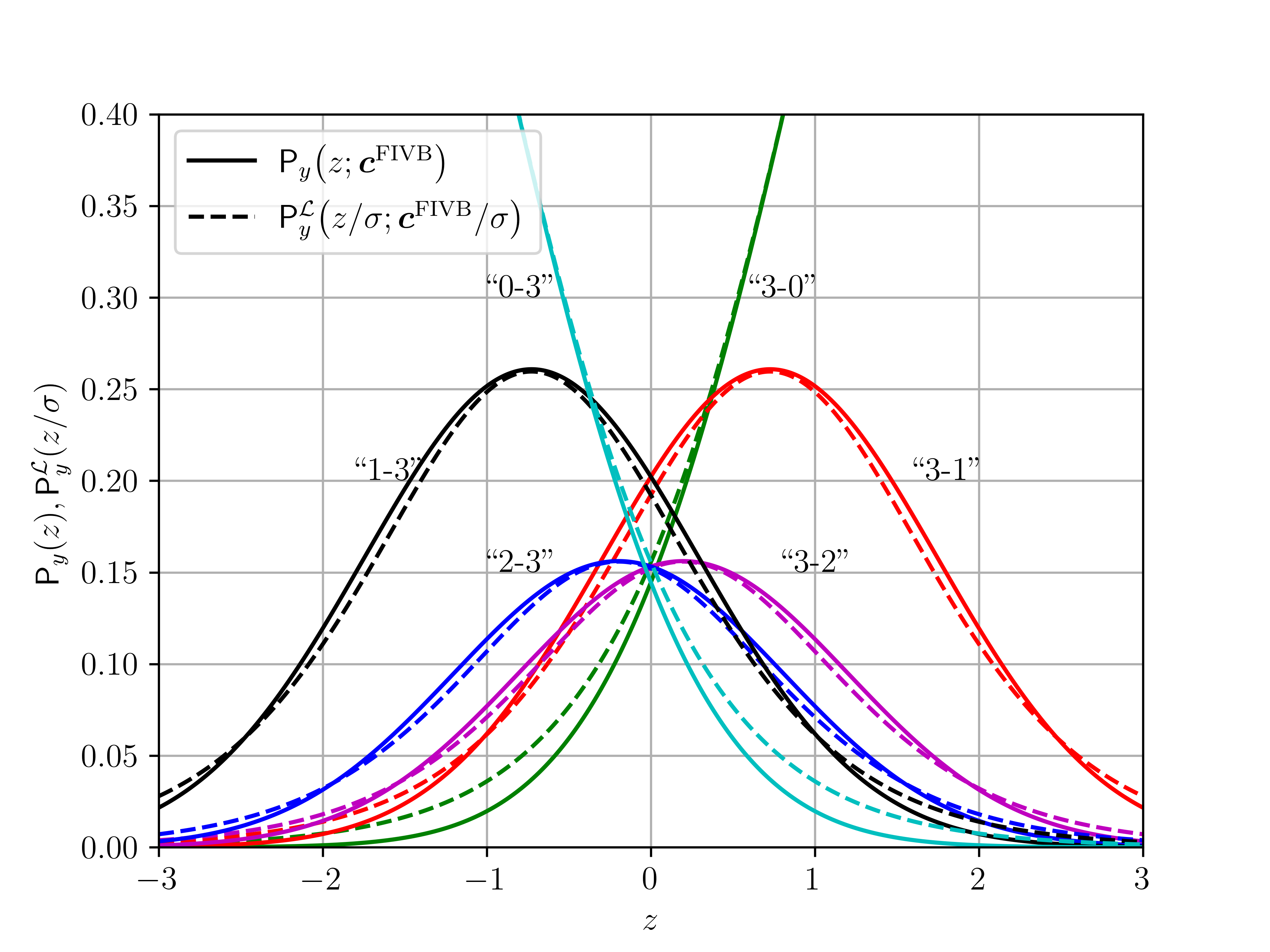
Figure 8: Models $\mathsf{P}_{y}(z;\boldsymbol{c})$ and $\mathsf{P}^{\mathcal{L}}_{y}(z/\sigma;\boldsymbol{c})$ defined respectively in (21) and (72), obtained from the Gaussian and the logistic CDF s; note the scaling by $\sigma$ applied in the latter.

To assess the CL model (72), we proceed as before, via optimization:

$$\hat{\boldsymbol{c}}^{\mathcal{L}},\hat{\eta}^{\mathcal{L}}=\mathop{\mathrm{argmin}}_{\boldsymbol{c},\eta}U(\boldsymbol{c},\eta,\boldsymbol{p}_{\backslash\{\boldsymbol{c},\eta\}}),$$ (79)

where the superscript $(\cdot)^{\mathcal{L}}$ is used to denote the parameters used in (72).

The ALO metrics are shown in Fig. 9, where the legend distinguishes the models (21) and (72) by indicating the CDF they use, i.e., $\Phi$ or $\mathcal{L}$. The results obtained using Gaussian CDF (i.e., $\Phi$) are reproduced from Fig. 3.

The main observations are the following:

• The CL logistic model, with the scaled version of the FIVB thresholds, $\boldsymbol{c}^{{\textnormal{FIVB}}}/\sigma$, outperforms the FIVB model. This is a notable result, obtained without any numerical optimization of the model parameters.

• Moreover, this choice of parameters is near-optimal. In fact, both the Gaussian and logistic CL models, yield similar performance after optimization.

The above observations indicate that, compared to the FIVB model, the CL logistic model is less sensitive to the imperfect parameter estimation which may be explained by heavier distribution tails of the logistic model; see Fig. 8.

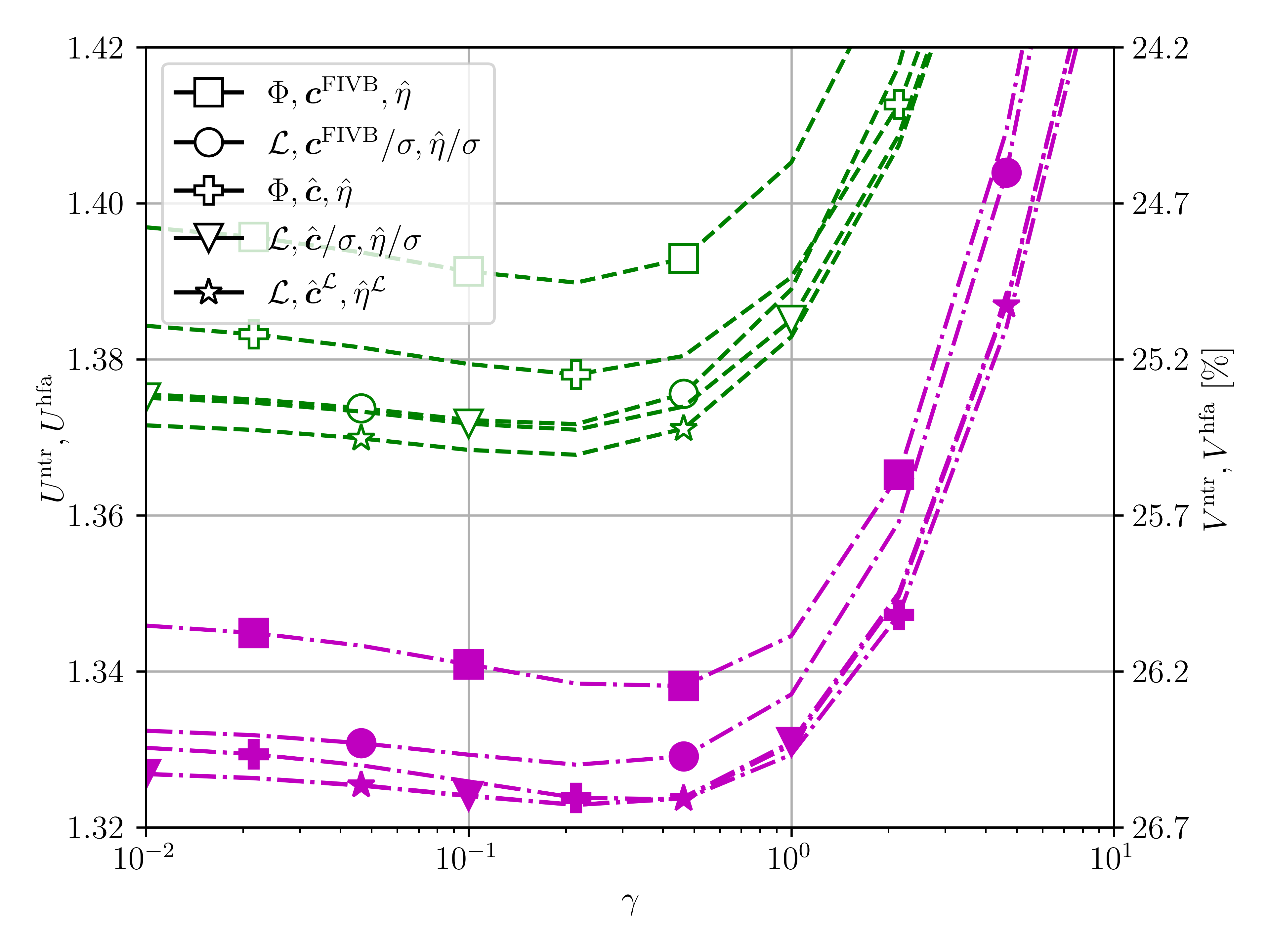
Figure 9: Validation metrics $U^{{\textnormal{ntr}}}$ (hollow markers) and $U^{{\textnormal{hfa}}}$ (colored markers) given by (57)-(58), shown as a function of $\gamma$ for the logistic CL model, (72) (and indicated with $\mathcal{L}$) are compared with the metrics obtained using the Gaussian CL model, (21) (and indicated with $\Phi$).

4.1 SG algorithm

The SG algorithm is obtained by finding the derivative of (73)

$$g^{\mathcal{L}}_{y}(z) =\dot{\ell}^{\mathcal{L}}_{y}(z)=\mathcal{L}(z+c_{y})+\mathcal{L}(z+c_{y-1})-1$$ (80)

$$=\mathcal{L}(z+c_{y-1})-\mathcal{L}(-z-c_{y}).$$ (81)

Since the implementation of (81) is straightforward, the SG rating algorithm

$$\hat{\boldsymbol{\theta}}_{t+1} \leftarrow\hat{\boldsymbol{\theta}}_{t}-\mu\boldsymbol{x}_{t}g^{\mathcal{L}}_{y_{t}}(\boldsymbol{x}_{t}^{\mathsf{T}}\hat{\boldsymbol{\theta}}_{t})$$ (82)

may be used directly without any numerical issues, and we note that it does not make any reference to the numerical scores, i.e., we do not need to assign any value to the observed outputs. This is exactly what we repeatedly said in this paper: ordinal results $y_{t}$, indeed, do not have any intrinsic value.

The interpretation of (82) is quite interesting. Namely, from (24), we know that $\Pr\left\{Y\leq y|z\right\}=\mathcal{L}(z+c_{y})$, and thus,

$$\mathcal{L}(z+c_{y-1})=\Pr\left\{Y<y|z\right\}$$ (83)

$$1-\mathcal{L}(z+c_{y})=\Pr\left\{Y>y|z\right\}$$ (84)

so, (81) becomes

$$g^{\mathcal{L}}_{y}(z) =\Pr\left\{Y<y|z\right\}-\Pr\left\{Y>y|z\right\}$$ (85)

$$=\Pr\left\{Y\leq y|z\right\}-\Pr\left\{Y\geq y|z\right\}.$$ (86)

Therefore, the algorithm (82) is driven by the difference between the right- and left-hand side distribution tails. Note that, the derivative $g^{\mathcal{L}}_{y_{t}}(z_{t})$ becomes null if the conditional distribution $\Pr\left\{Y_{t}|z_{t}\right\}$ has equal tails, or, equivalently, if $y_{t}$ is a perfect median of $Y_{t}$ (conditioned on $z_{t}$).

5 Real-time ranking

In previous sections, model evaluation relied on comparing analytically deduced parameters with those obtained through optimization. Our objective now is to directly use the model obtained thanks to analytical insights and to evaluate the performance of the real-time ranking based on the resulting SG algorithm.

We will thus keep the FIVB model defined by the threshold parameters $\boldsymbol{c}^{{\textnormal{FIVB}}}$ and evaluate i) the choice of the numerical score $\boldsymbol{r}$ used in the implicit loss function $\ell^{{\textnormal{FIVB}}}$, and specified in (66), ii) the values of the weights $\boldsymbol{\xi}$, see Sec. 3.4, and iii) the choice of the threshold parameters in the logistic CL model, see Sec. 4. Simply put, we do not carry out any explicit optimization of the model parameters when using the real-time ranking but, rather, rely on the parameters obtained from analysis. In this way, we avoid the contentious issue of choosing the model parameters from the data. The only exception is the choice of the HFA parameter which we set as $\eta=0.2$.

To initialize the SG algorithm (15), we use the skills $\theta_{m,0},m=1,\ldots,M$, where $\theta_{m,0}$ is read from the official FIVB ranking of the team $m$ at the time of their first game after 2020. By initializing the skills with those provided by the official ranking allows us to deal with the practical aspect of switching from one ranking (here, the official one) to another (the one we propose).

In order to switch the model from the Gaussian to the logistic CDF, we need to change the scaling, but this is also handled analytically: to obtain a quasi-equivalence of the model, the logistic model (72) needs to employ scaling $s^{\mathcal{L}}=\sigma s\approx 80$ (where $s=125$, see (21)) and use $\eta^{\mathcal{L}}=s/\sigma\approx 0.12$. Note that a similar strategy for adjusting the scales to avoid convergence problems is also discussed in (Szczecinski and Roatis, 2022, Sec. 5.1), but it is based on numerical results, while we do it analytically.

We calculate the validation metrics

$$\overline{U} =\frac{1}{T}\sum_{t=1}^{T}\ell^{{\textnormal{val}}}_{y_{t}}(\boldsymbol{x}_{t}^{\mathsf{T}}\hat{\boldsymbol{\theta}}_{t})$$ (87)

$$\overline{U}^{{\textnormal{ntr}}} =\frac{1}{T^{{\textnormal{ntr}}}}\sum_{\begin{subarray}{c}t=1\\ h_{t}=0\end{subarray}}^{T}\ell^{{\textnormal{val}}}_{y_{t}}(\boldsymbol{x}_{t}^{\mathsf{T}}\hat{\boldsymbol{\theta}}_{t})$$ (88)

$$\overline{U}^{{\textnormal{hfa}}} =\frac{1}{T^{{\textnormal{hfa}}}}\sum_{\begin{subarray}{c}t=1\\ h_{t}=1\end{subarray}}^{T}\ell^{{\textnormal{val}}}_{y_{t}}(\boldsymbol{x}_{t}^{\mathsf{T}}\hat{\boldsymbol{\theta}}_{t}).$$ (89)

These metrics are, in essence, equivalent to those shown in (57)-(58), which we have shown in the figures. The difference is that now skills $\hat{\boldsymbol{\theta}}_{t}$ are estimated using the SG algorithm.

The results obtained are shown in Table 5, where we indicate the loss function used (which determines the gradient used in the SG algorithm) and the parameters of the underlying model.

loss	parameters	$\mu$	$\overline{U}$	$\overline{U}^{{\textnormal{ntr}}}$	$\overline{U}^{{\textnormal{hfa}}}$	$\overline{\rho}$
$\ell^{{\textnormal{FIVB}}}$	$\boldsymbol{c}^{{\textnormal{FIVB}}},\boldsymbol{r}^{{\textnormal{FIVB}}},\boldsymbol{\xi}^{{\textnormal{FIVB}}},\eta=0$	0.01	1.52	1.51	1.53	0.94
		0.03	1.49	1.49	1.49	0.89
$\ell^{{\textnormal{FIVB}}}$	$\boldsymbol{c}^{{\textnormal{FIVB}}},\boldsymbol{r}^{{\textnormal{FIVB}}},\boldsymbol{\xi}^{{\textnormal{FIVB}}},\eta=0.2$	0.01	1.52	1.51	1.52	0.94
		0.03	1.48	1.49	1.47	0.89
$\ell^{{\textnormal{FIVB}}}$	$\boldsymbol{c}^{{\textnormal{FIVB}}},\tilde{\boldsymbol{r}},\boldsymbol{\xi}^{{\textnormal{FIVB}}},\eta=0.2$	0.01	1.52	1.51	1.53	0.94
		0.04	1.47	1.48	1.45	0.88
$\ell^{{\textnormal{FIVB}}}$	$\boldsymbol{c}^{{\textnormal{FIVB}}},\boldsymbol{r}^{{\textnormal{FIVB}}},\xi_{v}=1,\eta=0.2$	0.10	1.48	1.49	1.45	0.87
$\ell^{{\textnormal{FIVB}}}$	$\boldsymbol{c}^{{\textnormal{FIVB}}},\tilde{\boldsymbol{r}},\xi_{v}=1,\eta=0.2$	0.10	1.47	1.48	1.44	0.88
$\ell$	$\boldsymbol{c}^{{\textnormal{FIVB}}},\xi_{v}=1,\eta=0.2$	0.20	1.46	1.48	1.43	0.85
$\ell^{\mathcal{L}}$	$\boldsymbol{c}^{{\textnormal{FIVB}}}/\sigma,\xi_{v}=1,\eta=0.12,s=80$	0.40	1.45	1.46	1.42	0.88

Table 5: The metrics (87)-(89) obtained using the SG algorithm using different loss functions and parameters. We always show the results with the step $\hat{\mu}$ obtained via (90), except in the first three cases where we also show the results obtained using $\mu=0.01$ which is defined in the FIVB ranking.

For the algorithms based on the FIVB implicit loss function and the weighting with $\boldsymbol{\xi}^{{\textnormal{FIVB}}}$, we evaluate the performance using the nominal adaptation step $\mu=0.01$, and, for each algorithm, we also search for the adaptation step which minimizes the validation metric overall

$$\hat{\mu} =\mathop{\mathrm{argmin}}_{\mu}\overline{U}(\mu),$$ (90)

where $\overline{U}(\mu)=\overline{U}$ shown in (87).

To indicate how much the new algorithms change the ranking when comparing to the official FIVB ranking, we calculate the average Spearman correlation coefficient

$$\overline{\rho} =\frac{1}{T}\sum_{t=1}^{T}\rho(\boldsymbol{\theta}_{t}^{{\textnormal{FIVB}}},\hat{\boldsymbol{\theta}}_{t}),$$ (91)

where $\rho(\boldsymbol{\theta},\boldsymbol{\theta}^{\prime})$ is the Spearman correlation between the skill vectors $\boldsymbol{\theta}$ and $\boldsymbol{\theta}^{\prime}$.

Note that even using exactly the same parameters as the FIVB ranking (the first line in Table 5), our ranking is not the same as the official one because we discarded the forfeited games.

The results validate the observations we made analyzing the models. Namely, i) an improvement in performance is obtained using the parameter HFA $\eta=0.2$ and the numerical scores $\tilde{r}_{y}(\boldsymbol{c}^{{\textnormal{FIVB}}})$, see (65), and ii) the weighting with $\xi_{v}>1$ is counterproductive.

Regarding the choice of the adaptation step, we observe that

• The adaptation step $\mu=0.01$ used by the FIVB ranking seems too small and, by increasing it three- or four-fold, performance improves. This can be explained using the interpretation of the SG algorithm as a simplified Kalman filter (Szczecinski and Tihon, 2023, Sec. 3.3), where the adaptation step in the SG algorithm has a meaning of the posterior variance of the skills. In simple terms, the FIVB is over-optimistic about the uncertainty (variance) in the estimation of the skills.

• Since the weighting may also be interpreted as a variable step size, by removing it, i.e., using $\xi_{v}\equiv 1$, we have to explicitly increase the step size; this explains the large value of $\mu$ for each configuration in which we use $\xi_{v}=1$.

6 Conclusions

In this work, the online ranking algorithm used by the FIVB is presented in the statistical learning framework. To our best knowledge, the FIVB ranking is the first to adopt an explicit probabilistic model (here, the Cumulative Link (CL)model) of the multi-level ordinal outcomes, and, from the statistical perspective, this is a step in the right direction. On the other hand, the algorithms adopt simplifications which we demonstrate to be suboptimal, but we show how these may be easily corrected.

To analyze the algorithm, we use two approaches: i) the analytical, where the approximations and simplifications allow us to draw conclusions about the properties of the model, as well as to optimize its parameters, and ii) the numerical, where we explicitly optimize the parameters of the model from the outcomes of the international volleyball games used in the FIVB ranking.

The analytical approach is easily reproducible, while the numerical optimization which relies on the cross-validation strategy allows us to validate the insights obtained analytically.

The understanding of the FIVB ranking algorithm may be summarized as follows:

• The FIVB algorithm should be seen as the approximate ML inference of the skills from the ordinal game outcomes. The approximations are due to the use of the SG to solve the optimization problem, and, more importantly, due to the use of the loss functions, which are proxies for the log-likelihood of the ML approach. We explain the rationale for using such proxy loss functions.

• Although the form of loss functions is not explicitly mentioned in the description of the FIVB algorithm, they can be inferred from the equations, and we show how they depend on the numerical scores that are attributed to the ordinal game outcomes in the FIVB algorithm. This is interesting because in this way we explain the meaning of the numerical scores, as, from the modeling perspective, the ordinal variables do not have numerical values.

Regarding the model underlying the current FIVB algorithm, we studied its important elements:

• CL model thresholds $\boldsymbol{c}^{{\textnormal{FIVB}}}$, see (23), which define the probabilistic ordinal model of the data. They fit relatively well the data we analyzed (FIVB games from 2021-2023), see Sec. 3.2.

• Numerical scores $\boldsymbol{r}^{{\textnormal{FIVB}}}$, see Table 2, which define the algorithm. These are shown, both analytically and numerically, to be inadequately set, see Sec. 3.3.

• Importance weights $\boldsymbol{\xi}$, see Table 1, which change the contribution of the outcome of the game depending on the game type. These are shown to be irrelevant from an statistical point of view, see Sec. 3.4.

• Home-field advantage (HFA) which deals with the games played on the home venues by artificially boosting the skills of the home-team. Here, contrary to the statements in the FIVB descriptions, we found that the HFA is a relevant parameter that improves the prediction performance.

• CDF function, which defines the CL model, see (21). Replacing the Gaussian CDF used currently by the FIVB ranking with the logistic CDF, see (72), produces multiple benefits: i) the resulting algorithm is very simple, see (82) and (81), ii) it makes the concept of the numerical score superfluous, and iii) its thresholds $\boldsymbol{c}^{\mathcal{L}}$ can be obtained though a simple transformation of the thresholds $\boldsymbol{c}^{{\textnormal{FIVB}}}$ currently used in the FIVB ranking, see (78).

Recommendations

Since the FIVB explicitly says that its algorithm may be updated, if this is to happen, our recommendations are the following:

1. Introduce the HFA to the algorithm. This is a simple and low-cost modification, yielding an improvement in the prediction of the games played on the home-venue.

2. Change the numerical score $\boldsymbol{r}^{{\textnormal{FIVB}}}$ to be similar to those suggested in (66)-(68).

3. Remove the weighting of the games with $\xi^{{\textnormal{FIVB}}}_{v}$. Or, if its use is motivated by some extra-statistical reasons, decrease the differences between the possible values of $\xi_{v}^{{\textnormal{FIVB}}}$.

4. Use the logistic CDF in the CL model, as this removes the need for auxiliary numerical scores (thus making the recommendation #2 void) and yields a simple, and easily interpretable algorithm.

Appendix A Notation in FIVB ranking

We show in Table 6, the relationship between our notation and the one used in the FIVB ranking description FIVB (2024), where the following abbreviations are used

• WRS: World ranking score (here, we call it skills $\boldsymbol{\theta}_{m,t}$)

• SSV: Set score variant (we call it numerical score $r_{y}$)

• EMR: Expected match result (here, the expected score $\check{r}(z)$, see (27))

• MWF: Match weighting factor (here, it corresponds to $10\xi_{v_{t}}$)

• Scaled difference between scores $\Delta=8({\textnormal{WRS1}}-{\textnormal{WRS2}})/1000$

Our notation	FIVB notation
$\theta_{m,t},\theta_{n,t}$	WRS1, WRS2
$c_{0}^{{\textnormal{FIVB}}},\ldots,c_{4}^{{\textnormal{FIVB}}}$	C1, …, C5
$z_{t}/s=(\theta_{m,t}-\theta_{n,t})/s$	$\Delta=8({\textnormal{WRS1}}-{\textnormal{WRS2}})/1000$
$s$	1000/8=125
$\mathsf{P}_{0}(z_{t}),\ldots,\mathsf{P}_{5}(z_{t})$	P1, …, P5
$\Phi(z)$	$\sim N(0,1)(z)$
$r_{y_{t}}^{{\textnormal{FIVB}}}$	SSV
$\check{r}(z_{t}/s)$	EMR
$10\xi_{v_{t}}$	MWF
$-g^{{\textnormal{FIVB}}}(z_{t}/s)=r_{y_{t}}^{{\textnormal{FIVB}}}-\check{r}(z_{t}/s)$	WR value
$\theta_{m,t+1}-\theta_{m,t}=-10\xi_{v_{t}}g^{{\textnormal{FIVB}}}(z_{t}/s)$	WR points = WR values * MWF /8

Table 6: Equivalence of this work’s notation and the one used in the description of the FIVB ranking.

With this notation, the update formula is given by

$$\text{WRS1}\leftarrow\text{WRS1}+\text{WR points}$$ (92)

and corresponds to (25) which, focusing on the update of the skills of the home team $m$, may be written as

$$\theta_{m,t+1} =\theta_{m,t}-\mu s\xi_{v_{t}}g^{{\textnormal{FIVB}}}_{y_{t}}(z_{t}/s).$$ (93)

Appendix B Optimization of the cross-validation metric

The simplest optimization of the cross-validation metric $U(\boldsymbol{p})$ may be done via the steepest descent

$$\hat{\boldsymbol{p}}\leftarrow\hat{\boldsymbol{p}}-\kappa\nabla_{\boldsymbol{p}}U(\boldsymbol{p}),$$ (94)

where, $\kappa$ is the step-size, and to calculate the gradient $\nabla_{\boldsymbol{p}}U(\boldsymbol{p})$, we have to calculate derivatives of $U(\boldsymbol{p})$ with respect to a parameter $q\in\boldsymbol{p}$. This can be done as follows:

$$\frac{\partial}{\partial q}U(\boldsymbol{p}) =\frac{1}{T}\sum_{t=1}^{T}\frac{\partial}{\partial q}\ell^{{\textnormal{val}}}_{y_{t}}(\hat{z}_{t,\backslash{t}},\boldsymbol{p})$$ (95)

$$\frac{\partial}{\partial q}\ell^{{\textnormal{val}}}_{y_{t}}(\hat{z}_{t,\backslash{t}}) =\frac{\partial\hat{z}_{t,\backslash{t}}}{\partial q}\dot{\ell}^{{\textnormal{val}}}(\hat{z}_{t,\backslash{t}},\boldsymbol{p})+\frac{\partial}{\partial q}\ell^{{\textnormal{val}}}_{y_{t}}(\hat{z}_{t,\backslash{t}},\boldsymbol{p})$$ (96)

$$\frac{\partial\hat{z}_{t,\backslash{t}}}{\partial q} =\frac{\partial\hat{z}_{t}}{\partial q}+\frac{\partial}{\partial q}\left[\frac{\xi_{v_{t}}\dot{\ell}_{y_{t}}(\hat{z}_{t},\boldsymbol{p})a_{t}}{1-\xi_{v_{t}}\ddot{\ell}_{y_{t}}(\hat{z}_{t},\boldsymbol{p})a_{t}}\right].$$ (97)

In (97), we will need

$$\frac{\partial\hat{z}_{t}}{\partial q} =\boldsymbol{x}^{\mathsf{T}}_{t}\frac{\partial\hat{\boldsymbol{\theta}}}{\partial q}$$ (98)

$$\frac{\partial a_{t}}{\partial q} =\boldsymbol{x}^{\mathsf{T}}_{t}\frac{\partial\hat{{\textnormal{{H}}}}^{-1}}{\partial q}\boldsymbol{x}_{t}=-\boldsymbol{x}^{\mathsf{T}}_{t}\hat{{\textnormal{{H}}}}^{-1}\frac{\partial\hat{{\textnormal{{H}}}}}{\partial q}\hat{{\textnormal{{H}}}}^{-1}\boldsymbol{x}_{t}$$ (99)

$$\frac{\partial\hat{\textnormal{{H}}}}{\partial q} =\sum_{t=1}^{T}\boldsymbol{x}_{t}\frac{\partial}{\partial q}\big{[}\xi_{v_{t}}\ddot{\ell}_{y_{t}}(\hat{z}_{t},\boldsymbol{p})\big{]}\boldsymbol{x}^{\mathsf{T}}_{t}+\mathds{I}\big{[}{q=\gamma}\big{]}{\textnormal{{I}}}$$ (100)

$$\frac{\partial}{\partial q}\dot{\ell}_{y_{t}}(\hat{z}_{t},\boldsymbol{p}) =\frac{\partial\hat{z}_{t}}{\partial q}\ddot{\ell}_{y_{t}}(\hat{z}_{t},\boldsymbol{p})+\frac{\partial}{\partial q}\dot{\ell}_{y_{t}}(\hat{z}_{t},\boldsymbol{p})$$ (101)

$$\frac{\partial}{\partial q}\ddot{\ell}_{y_{t}}(\hat{z}_{t},\boldsymbol{p}) =\frac{\partial\hat{z}_{t}}{\partial q}\dddot{\ell}_{y_{t}}(\hat{z}_{t},\boldsymbol{p})+\frac{\partial}{\partial q}\ddot{\ell}_{y_{t}}(\hat{z}_{t},\boldsymbol{p})$$ (102)

where, in (99) we used (Petersen and Pedersen, 2012, Eq. (40)), and $\dddot{\ell}_{y}(z,\boldsymbol{p})=\frac{\partial^{3}}{\partial z^{3}}\ell_{y}(z,\boldsymbol{p})$.

From implicit function theorem, see (Lorraine et al., 2019, Th. 1), using $\hat{\boldsymbol{\theta}}\equiv\hat{\boldsymbol{\theta}}(\boldsymbol{p})$

$$\boldsymbol{0} =\frac{\partial}{\partial q}\Big{[}\nabla_{\boldsymbol{\theta}}J(\hat{\boldsymbol{\theta}}(\boldsymbol{p}),\boldsymbol{p})\Big{]}$$ (103)

$$\boldsymbol{0} =\nabla^{2}_{\boldsymbol{\theta}}J(\hat{\boldsymbol{\theta}}(\boldsymbol{p}),\boldsymbol{p})\frac{\partial\hat{\boldsymbol{\theta}}(p)}{\partial q}+\frac{\partial}{\partial q}\nabla_{\boldsymbol{\theta}}J(\hat{\boldsymbol{\theta}},\boldsymbol{p})$$ (104)

$$\frac{\partial\hat{\boldsymbol{\theta}}}{\partial q} =-\hat{{\textnormal{{H}}}}^{-1}\frac{\partial}{\partial q}\nabla_{\boldsymbol{\theta}}J(\hat{\boldsymbol{\theta}},\boldsymbol{p})$$ (105)

$$\frac{\partial}{\partial q}\nabla_{\boldsymbol{\theta}}J(\hat{\boldsymbol{\theta}},\boldsymbol{p}) =\sum_{t=1}^{T}\frac{\partial}{\partial q}\big{[}\xi_{v_{t}}\dot{\ell}_{y_{t}}(\boldsymbol{x}_{t}^{\mathsf{T}}\hat{\boldsymbol{\theta}},\boldsymbol{p})\big{]}\boldsymbol{x}_{t}+\mathds{I}\big{[}{\gamma=q}\big{]}\hat{\boldsymbol{\theta}}.$$ (106)

By plugging $\hat{z}_{t,\backslash{t}}(\boldsymbol{p})$ into (39) we obtain the function $U(\boldsymbol{p})$ which depends on $\boldsymbol{p}$ and we can calculate the gradient $\nabla_{\boldsymbol{p}}U(\boldsymbol{p})$.

Similarly, we can use the Newton method

$$\hat{\boldsymbol{p}}\leftarrow\hat{\boldsymbol{p}}-[\nabla^{2}_{\boldsymbol{p}}U(\boldsymbol{p})]^{-1}\nabla_{\boldsymbol{p}}U(\boldsymbol{p})$$ (107)

where, to calculate the Hessian, $\nabla^{2}_{\boldsymbol{p}}U(\boldsymbol{p})$ we need second order derivatives.

However, the expressions for the gradient and, especially, the Hessian, quickly become cumbersome; see Burn (2020). Thus, instead of explicit differentiation, we use the automatic differentiation available in JAX and JAXopt python-compliant packages Bradbury et al. (2018), Blondel et al. (2021) with a particularly interesting feature of implicit differentiation required to find the derivative of $\hat{\boldsymbol{\theta}}$ with respect to hyperparameters in $\boldsymbol{p}$ as specified by (105).

We do not show more details to not overcomplicate the presentation, especially that they are not really required because the numerical optimization is used to confirm the observation we made using the analytical insight. In fact, the performance of the online algorithm shown in Sec. 5 uses the parameters (shown in Table 5) which are explicitly defined prior to the application of the algorithms.

References

- Aldous (2017) Aldous, D. (2017): “Elo ratings and the sports model: A neglected topic in applied probability?” Statist. Sci., 32, 616–629, URL https://doi.org/10.1214/17-STS628.
- Barber (2012) Barber, D. (2012): Bayesian reasoning and Machine Learning, Cambridge University Press.
- Beirami et al. (2017) Beirami, A., M. Razaviyayn, S. Shahrampour, and V. Tarokh (2017): “On optimal generalizability in parametric learning,” in Proceedings of the 31st International Conference on Neural Information Processing Systems, NIPS’17, Red Hook, NY, USA: Curran Associates Inc., 3458–3468.
- Blondel et al. (2021) Blondel, M., Q. Berthet, M. Cuturi, R. Frostig, S. Hoyer, F. Llinares-López, F. Pedregosa, and J.-P. Vert (2021): “Efficient and modular implicit differentiation,” arXiv preprint arXiv:2105.15183.
- Bradbury et al. (2018) Bradbury, J., R. Frostig, P. Hawkins, M. J. Johnson, C. Leary, D. Maclaurin, G. Necula, A. Paszke, J. VanderPlas, S. Wanderman-Milne, and Q. Zhang (2018): “JAX: composable transformations of Python+NumPy programs,” URL http://github.com/google/jax.
- Burn (2020) Burn, R. (2020): “Optimizing approximate leave-one-out cross-validation to tune hyperparameters,” ArXiv, abs/2011.10218, URL http://arxiv.org/abs/2011.10218.
- Csató (2024) Csató, L. (2024): “Club coefficients in the UEFA champions league: Time for shift to an Elo-based formula,” International Journal of Performance Analysis in Sport, 24, 119–134, URL https://doi.org/10.1080/24748668.2023.2274221.
- Elo (2008) Elo, A. E. (2008): The Rating of Chess Players, Past and Present, Ishi Press International.
- FIVB (2024) FIVB (2024): “Fivb volleyball world ranking,” URL https://en.volleyballworld.com/volleyball/world-ranking/ranking-explained.
- Gomes de Pinho Zanco et al. (2024) Gomes de Pinho Zanco, D., L. Szczecinski, E. Vinicius Kuhn, and R. Seara (2024): “Stochastic analysis of the Elo rating algorithm in round-robin tournaments,” Digital Signal Processing, 145, 104313, URL https://www.sciencedirect.com/science/article/pii/S1051200423004086.
- Hastie et al. (2009) Hastie, T., R. Tibshirani, and J. Friedman (2009): The Elements of Statistical Learning, Springer Series in Statiscs.
- Hu and Zidek (2001) Hu, F. and J. V. Zidek (2001): The Relevance Weighted Likelihood With Applications, New York, NY: Springer New York, 211–235, URL https://doi.org/10.1007/978-1-4613-0141-7_13.
- Jabin and Junca (2015) Jabin, P.-E. and S. Junca (2015): “A continuous model for ratings,” SIAM J. Appl. Math, 2, 420–442, URL https://doi.org/10.1137/140969324.
- Ley et al. (2019) Ley, C., T. Van de Wiele, and H. Van Eetvelde (2019): “Ranking soccer teams on the basis of their current strength: A comparison of maximum likelihood approaches,” Statistical Modelling, 19, 55–73, URL https://doi.org/10.1177/1471082X18817650.
- Lorraine et al. (2019) Lorraine, J., P. Vicol, and D. Duvenaud (2019): “Optimizing millions of hyperparameters by implicit differentiation,” CoRR, abs/1911.02590, URL http://arxiv.org/abs/1911.02590.
- Petersen and Pedersen (2012) Petersen, K. B. and M. S. Pedersen (2012): “The matrix cookbook,” URL http://www2.compute.dtu.dk/pubdb/pubs/3274-full.html, version 20121115.
- Rad and Maleki (2020) Rad, K. R. and A. Maleki (2020): “A scalable estimate of the out-of-sample prediction error via approximate leave-one-out cross-validation,” Journal of the Royal Statistical Society: Series B (Statistical Methodology), 82, 965–996, URL https://rss.onlinelibrary.wiley.com/doi/abs/10.1111/rssb.12374.
- Szczecinski and Djebbi (2020) Szczecinski, L. and A. Djebbi (2020): “Understanding draws in Elo rating algorithm,” URL https://www.degruyter.com/document/doi/10.1515/jqas-2019-0102/html.
- Szczecinski and Roatis (2022) Szczecinski, L. and I.-I. Roatis (2022): “FIFA ranking: Evaluation and path forward,” Journal of Sports Analytics, 8, 231–250, URL https://content.iospress.com/articles/journal-of-sports-analytics/jsa200619.
- Szczecinski and Tihon (2023) Szczecinski, L. and R. Tihon (2023): “Simplified Kalman filter for online rating: one-fits-all approach,” Journal of Quantitative Analysis in Sports, URL http://arxiv.org/abs/2104.14012,https://doi.org/10.1515/jqas-2021-0061.
- Tutz (2012) Tutz, G. (2012): Regression for categorical data, Cambridge University Press.