Physics-Informed Geometry-Aware Neural Operator

Abstract

Engineering design problems often involve solving parametric Partial Differential Equations (PDEs) under variable PDE parameters and domain geometry. Recently, neural operators have shown promise in learning PDE operators and quickly predicting the PDE solutions. However, training these neural operators typically requires large datasets, the acquisition of which can be prohibitively expensive. To overcome this, physics-informed training offers an alternative way of building neural operators, eliminating the high computational costs associated with Finite Element generation of training data. Nevertheless, current physics-informed neural operators struggle with limitations, either in handling varying domain geometries or varying PDE parameters. In this research, we introduce a novel method, the Physics-Informed Geometry-Aware Neural Operator (PI-GANO), designed to simultaneously generalize across both PDE parameters and domain geometries. We adopt a geometry encoder to capture the domain geometry features, and design a novel pipeline to integrate this component within the existing DCON architecture. Numerical results demonstrate the accuracy and efficiency of the proposed method.

Keywords Physics-informed deep learning, Neural operator, Geometry generalization

1 Introduction

Numerical solution of partial differential equations (PDEs) has been a very active field of research in the last recent, when in particular Finite Element Method (FEM) was primarily studied. FEM involves discretizing a continuous function space using a discrete mesh and solving high-dimensional a linear system, which can be computationally demanding Dhatt et al. (2012). This computational cost becomes particularly substantial in tasks requiring repetitive solutions. An example of such tasks is engineering design which necessitates solving parameterized PDEs over a wide range of PDE parameters and domain geometries for design evaluation Almasri et al. (2024).

Recently, machine learning techniques have been introduced to accelerate the process of solving PDEs by learning a neural operator as a mapping from variable PDE parameters and/or domain geometry to the PDE solution Lu et al. (2021). Once a neural operator model is successfully trained on a dataset, it can generalize to new, unseen parameters and domain geometries. This is done by a single forward pass through the trained neural network, with minimal computational cost.

Research on neural operators initially was focused on developing various neural operator architectures for operator learning of parametric PDEs in a data-driven way Lu et al. (2021); Li et al. (2020a); Kovachki et al. (2021); Li et al. (2020b). As the first neural operator architecture, Deep Operator Networks (DeepONet) Lu et al. (2021) utilize the universal approximation theorem for operators, introducing an architecture that approximates nonlinear operators through learning a collection of basis functions and coefficients. The Fourier Neural Operator (FNO) Li et al. (2020a) leverages the Fourier transform to model mappings in the spectral domain, capturing global dependencies and showing superior performance in square domain shapes. Geo-FNO Li et al. (2023) extends FNO to irregular meshes by learning a mapping from an irregular mesh to a uniform mesh. Inspired by FNO, Wavelet Neural Operator (WNO) Tripura and Chakraborty (2022) is also proposed by using wavelet transform instead of Fourier transform to better handle signals with discontinuity and spikes in an irregular domain geometry. While each of these methods has demonstrated potential in specific applications, a common limitation is that each trained model is restricted to a specific domain geometry.

To overcome the limitations of these “geometry-specific" methods, a number of “geometry aware" methods have been developed. The Graph Neural Operator (GNO) Li et al. (2020b) employs graph neural networks (GNNs) for operator learning by treating inputs and outputs as graphs, enabling generalization across different domain geometries. Similarly, PointNet Wang et al. (2024) facilitates PDE operator learning across diverse geometries by using a set of collocation points to represent the domain geometry. As an extension of FNO, geometry-aware FNO Li et al. (2024) was proposed for PDE solution prediction using a signed distance function (SDF) and point-cloud representations of the geometry. Diffeomorphism Neural Operator Zhao et al. (2024) combines harmonic mapping approach and the FNO to offer geometry generalization ability to FNO. Additionally, the General Neural Operator Transformer (GNOT) Hao et al. (2023) encodes the PDE parameters and domain geometries into tokens and adopt the architecture of Transformer Vaswani et al. (2017) for PDE solution predictions. Using the same idea of GNOT, other transformer-based methods Wu et al. (2024); Hemmasian and Farimani (2024); Lee and Oh (2024) were also proposed to address PDEs in varying geometrical settings.

Even though these methods offer the ability of generalizing to various PDE parameters and geometries, they all are data-intensive Wang et al. (2021). To bypass the need for training datasets, which are typically expensive to obtain, physics-informed neural operators, which are inspired by physics-informed neural networks (PINNs) Raissi et al. (2019), have emerged as an effective approach. This approach integrates the governing PDEs directly into the training process, making it possible to develop a neural operator without any training data obtained from high fidelity simulations, such as FEM. Among these methods, Physics-informed DeepONet (PI-DeepONet) Wang et al. (2021) extends the original DeepONet framework by embedding physical laws directly into the loss function with automatic differentiation Van Merriënboer et al. (2018) during training, which can only be applied on a specific mesh. Physics-informed Fourier Neural Operator (PI-FNO) Li et al. (2021) builds upon the original FNO framework, offering generalization across different PDE parameter representations in a square domain while also incorporating physics-informed training methods. Similarly, physics-informed Wavelet Neural Operator (PI-WNO) Navaneeth et al. (2024) is also proposed based on the architecture of WNO, implementing physics-informed training for WNO Tripura and Chakraborty (2022) using stochastic projection. Physics-informed Deep Compositional Operator Network (PI-DCON) Zhong and Meidani (2024) adopts a pooling layer to capture the global features of the variable PDE parameters, which enable the learning the PDE operator on any given irregular domain geometry. However, all these physics-informed methods struggle with generalization to varying geometries. A significant advancement to address this limitation is the Physics-informed PointNet (PI-PointNet) Kashefi and Mukerji (2022), which integrates a physics-informed training algorithm into PointNet. Nonetheless, PI-PointNet lacks the capability to generalize across PDE parameters, which limits its application in tackling complex problems in engineering design which also involves varying boundary conditions, etc.

In this study, we tackle the aforementioned challenges by introducing an innovative framework, called Physics-informed Geometry-aware Neural Operator (PI-GANO). This model is inspired by PI-DCON and PI-PointNet and is capable of generalizing across different PDE parameter representations and domain geometry representations simultaneously, including those in irregular domain shapes. The differences between our proposed model versus other existing works are summarized in Table LABEL:table.archi_compare. To the best of our knowledge, our proposed model is the first attempt to develop a neural operator that can simultaneously handle varying PDE parameters and domain geometries without need for any training data.

Table 1: Differences of Physics-informed Geometry-aware Neural Operator versus other existing models.

	Data-free	Generalize across PDE parameter representations	Generalize across geometries
DeepONet	✗	✗	✗
FNO, WNO ,LRNO geo-FNO	✗	✔	✗
GNO , GNOT, GA-FNO, Diff-NO	✗	✔	✔
PI-DeepONet	✔	✗	✗
PI-FNO, PI-WNO, PI-DCON	✔	✔	✗
PI-PointNet	✔	✗	✔
PI-GANO	✔	✔	✔

The remainder of this paper is organized as follows. In Section 2, we briefly introduce the problem settings and technical backgrounds for PI-DeepONet and PI-PointNet. Section 3 introduces our model architecture and explains the key points about it. Finally, numerical experiments and detailed performance evaluation of the proposed methods and conclusions are included in Sections 4 and 5.

2 Technical background

2.1 Problem Setting

Our goal is to develop an efficient machine learning-based solver for parametric PDEs which are formulated by:

$$\mathcal{N}_{\bm{x}}[u(\bm{x}),k(\bm{x})] =0,\quad \bm{x}\in\Omega,$$ (1)

$$\mathcal{B}_{\bm{x}}[u(\bm{x})] =g(\bm{x}),\quad \bm{x}\in\partial\Omega,$$

where $\Omega$ is a physical domain in $R^{d}$, $\bm{x}$ is a $d$-dimensional vector of spatial coordinates, $\mathcal{N}_{\bm{x}}$ is a general differential operator, and $\mathcal{B}_{\bm{x}}$ is a boundary conditiond operator acting on the domain boundary $\partial\Omega$. Also, $k(\bm{x})$ refers to the parameters of the PDE, which can include the coefficients and forcing terms in the governing equation, $g(\bm{x})$ denotes the boundary conditions, and $u(\bm{x})$ is the solution of this PDE for a given set of parameters and boundary conditions.

We seek to solve this PDE across different parameters and geometries. Let $\bm{\Omega}=\{\Omega_{1},\Omega_{2},...,\Omega_{n}\}$ denote the set of variable geometries. For each geometry $\Omega_{i}$, we have a corresponding set of PDE parameters, i.e. coefficients denoted by $k_{i}(\bm{x})$ and boundary conditions denoted by $g_{i}(\bm{x})$. Therefore, we employ a neural network model to approximate the operator $\mathcal{M}$ defined by:

$$\mathcal{M}:\{k_{i}(\bm{x}),g_{i}(\bm{x}),\Omega_{i}\}\rightarrow u_{i}(\bm{x}),\quad\bm{x}\in\Omega_{i},\quad\Omega_{i}\in\bm{\Omega},$$ (2)

where the inputs to the operator include information on both PDE parameters and domain geometries. Existing physics-informed neural operators primarily focus on learning the PDE operator with variations in either the PDE parameters or geometry. Our proposed framework handles both of these variation types. This is done by using two model ingredients: (1) one based on PI-DeepONet to handle varying PDE parameters and (2) one inspired by PI-PointNet to encode varying domain geometries. In the next two sections, we present the background for PI-DeepONet and PI-PointNet.

2.2 Parameter encoding with physics-informed DeepONet

DeepONet was proposed to solve parametric PDEs by approximating a domain-specific operator $\mathcal{M}$ given by

$$\mathcal{M}:\{k_{i}(\bm{x}),g_{i}(\bm{x})\}\rightarrow u_{i}(\bm{x}),\quad\bm{x}\in\Omega$$ (3)

where $\Omega$ is a given domain geometry. Specifically, DeepONet approximates $\mathcal{M}$ by a neural network model $\mathcal{U}_{\theta}(\bm{x},k(\bm{x}^{\prime}),g(\bm{x}^{\prime\prime}))$, where $\bm{x}$ denotes the coordinates at which the solution $u$ is to be calculated, and $\bm{x}^{\prime}$ and $\bm{x}^{\prime\prime}$ denote the coordinates at which the values of coefficients and boundary conditions, respectively, are available.

As shown in Figure  1, the architecture of DeepONet is composed of two separate neural networks referred to as the “branch net" and “trunk net", respectively. Both the branch net and trunk net are simply multilayer perceptrons (MLP). The DeepONet prediction is given by

$$\mathcal{U}_{\theta}(\bm{x},k(\bm{x}^{\prime}),g(\bm{x}^{\prime\prime}))=\sum_{i}^{q}b_{i}t_{i}.$$ (4)

where the $q$-dimensional features embedding $\bm{b}=[b_{1},b_{2},...,b_{q}]$ is the output of the branch net, and the $q$-dimensional coordinate embedding $\bm{t}=[t_{1},t_{2},...,t_{q}]$ is the output of the trunk neural networks. To calculate $\bm{t}$, the trunk net takes the coordinates of a collocation point, $\bm{x}$, as input. To calculate $\bm{b}$, the branch net takes $[k(\bm{x}^{\prime}_{1}),k(\bm{x}^{\prime}_{2}),...,k(\bm{x}^{\prime}_{l}),g(\bm{x}^{\prime\prime}_{1}),g(\bm{x}^{\prime\prime}_{2}),\cdots,g(\bm{x}^{\prime\prime}_{m})]$ as input. This input is the parameter function $k(\bm{x}^{\prime})$ evaluated at a collection of sampled locations $\{\bm{x}^{\prime}_{j}\}_{j=1}^{l}$ and the boundary function $g(\bm{x}^{\prime\prime})$ evaluated at a generally different collection of sampled locations $\{\bm{x}^{\prime\prime}_{j}\}_{j=1}^{m}$.

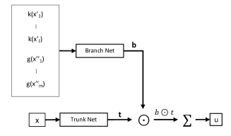
Figure 1: The architecture of the DeepONet is shown.

In order to set up the training loss for the model training, we first obtain $N$ realizations of branch net input, where each realization is parameter function $k(\cdot)$ obtained at locations $\bm{x}^{\prime}$ and BC function $g(\cdot)$ obtained at locations $\bm{x}^{\prime\prime}$. Then the physics-informed training loss of the neural operator $\mathcal{L}_{\text{PINO}}$ is given by:

$$\mathcal{L}_{\text{PINO}}=\mathcal{L}_{\text{PDE}}+\alpha\mathcal{L}_{\text{BC}}$$ (5)

where

$$\mathcal{L}_{\text{PDE}} =\frac{1}{N}\sum_{i}^{N}(\mathcal{N}_{\bm{x}}[\mathcal{U}_{\theta}(\bm{x},k_{i}(\bm{x}^{\prime}),g_{i}(\bm{x}^{\prime\prime})),k_{i}(\bm{x}^{\prime})])^{2},\quad \bm{x}\in\Omega,$$ (6)

$$\mathcal{L}_{\text{BC}} =\frac{1}{N}\sum_{i}^{N}(\mathcal{B}_{\bm{x}}[\mathcal{U}_{\theta}(\bm{x},k_{i}(\bm{x}^{\prime}),g_{i}(\bm{x}^{\prime\prime}))]-g_{i}(\bm{x}^{\prime\prime}))^{2},\quad \bm{x}\in\partial\Omega,$$

where $\alpha$ is the trade-off coefficient between the PDE residual loss term and the initial and boundary condition loss term. The optimal neural network parameters $\theta$ are found by minimizing the total training loss $\mathcal{L}_{\text{PINO}}$ with exact derivatives computed using automatic differentiation Van Merriënboer et al. (2018). After the model training, for any new realization of the parameters, the well-trained DeepONet can predict the corresponding solution directly in a specific domain geometry $\Omega$. To ensure the efficiency of model training, we implement stochastic gradient descent algorithm to update model parameters by random sampling of collocation points in each epoch.

2.3 Geometry encoding with physics-informed PointNet

PI-PointNet focus on approximating the PDE operator across a set of domain geometries. In its original form, it does not handle varying PDE parameters. Specifically, let the operator $\mathcal{M}$ be given by

$$\mathcal{M}:\{\Omega_{i}\}\rightarrow u_{i}(\bm{x}),\quad\bm{x}\in\Omega_{i},\quad\Omega_{i}\in\bm{\Omega}.$$ (7)

Each domain geometry $\Omega_{i}$ is represented by a set of $s_{i}$ collocation points inside the domain, denoted by $\{\bm{x}_{j}\}_{j=1}^{s_{i}}$. PI-PointNet takes these coordinates as input, and predicts the PDE solution on the input collocation points $\{u(\bm{x}_{i})\}_{i=1}^{s_{i}}$. The model parameters are estimated in a physics-informed training using the same loss function shown in Equation 5.

The architecture of the PointNet consists of two multilayer perceptrons $\mathcal{U}_{1}(\cdot,\theta_{1})$ and $\mathcal{U}_{2}(\cdot,\theta_{2})$, where $\theta_{1}$ and $\theta_{2}$ are trainable parameters. For each geometry input $\Omega_{i}$, it first generates the hidden embeddings $\bm{h}$ of the input collocation points by:

$$\{\bm{h}_{j}\}_{j=1}^{s_{i}}=\{\mathcal{U}_{1}(\bm{x}_{j},\theta_{1})\}_{j=1}^{s_{i}}.$$ (8)

Then a Maxpooling layer Gholamalinezhad and Khosravi (2020) is applied to hidden embeddings to obtain a global feature $\bm{G}^{i}$ of the $i$-th geometry:

$$\bm{G}^{i}=\text{Maxpool}(\{\bm{h}_{j}\}_{j=1}^{s_{i}}),$$ (9)

where Maxpool refers to the max-pooling operation which calculates the maximum value in each embedding dimension over all the $s_{i}$ points. The global feature is then concatenated to each of the hidden embeddings, providing a unique embedding $\bm{H}^{i}_{j}$ of coordinate $\bm{x}_{j}$ in the $i$-th geometry by

$$\bm{H}^{i}_{j}=[\bm{h}_{j}\|{g}^{i}].$$ (10)

The final PDE solution over the whole domain $\{u(\bm{x}_{i})\}_{i=1}^{s_{i}}$ is computed by

$$\{u_{i}(\bm{x}_{j})\}_{j=1}^{s_{i}}=\{\mathcal{U}_{2}(\bm{H}^{i}_{j},\theta_{2})\}_{j=1}^{s_{i}}.$$ (11)

3 Methodology

In this section, we introduce our proposed Physics-informed Geometry-aware Neural Operator (PI-GANO) for PDE operator learning. Our approach is primarily based on the PI-DCON architecture and draws inspiration from PI-PointNet. We will first explain the architecture of DCON in Section 3.1, followed by a detailed discussion of our inspiration and methodological innovations in Section 3.2. In Section 3.3, we will also highlight the main novelties of our method by comparing it with PI-PointNet.

3.1 Deep Compositional Operator Network

Our model is built upon on the architecture of Deep Compositional Operator Network Zhong and Meidani (2024). Without loss of generality, let us consider a simplistic case where the variability is only in one parameter, here denoted by $g(\bm{x})$. Our goal is then to find an approximation for the following operator,

$$\mathcal{M}:\{g(\bm{x}),\Omega\}\rightarrow u(\bm{x}),\quad\bm{x}\in\Omega.$$ (12)

We can approximate this PDE operator with the architecture of Deep Compositional Operator Network (DCON). Using DCON, the PDE parameters are represented in a discrete form by evaluating function $g$ on a finite number of sampled coordinates $[\bm{x}^{\prime}_{1},\bm{x}^{\prime}_{2},...,\bm{x}^{\prime}_{m}]$, i.e. $\bm{g}=[g(\bm{x}^{\prime}_{1}),g(\bm{x}^{\prime}_{2}),\cdots,g(\bm{x}^{\prime}_{m})]$. A multi-layer perceptron, $\mathcal{U}_{b}(\cdot,\theta_{b})$, is applied to it with a Max-pooling layer to derive the low-dimensional feature embedding $\bm{b}$ by:

$$\bm{b}=\text{Maxpool}(\{\mathcal{U}_{b}(g(\bm{x}^{\prime}_{j}),\theta_{b})\}_{j=1}^{m}),$$ (13)

where $\theta_{b}$ are trainable parameters. After computing the parameter embedding $\bm{b}$, the PDE operator $\mathcal{M}$ is approximated by a compositional version of DeepONet Lu et al. (2021) with multiple stacked operator layers $\{\mathcal{O}_{j}\}$

$$\mathcal{M}\approx\mathcal{M}_{\theta}=\text{sum}\{\bm{b}\odot...\ \mathcal{O}_{2}(\bm{b}\odot\mathcal{O}_{1}(\bm{b}\odot\bm{t}(\bm{x})))\},$$ (14)

where $\theta$ denotes all the trainable parameters of the operator layers, described later, $\odot$ refers to component-wise multiplication, $\bm{t}:\mathbb{R}^{d}\rightarrow\mathbb{R}^{q}$ is a learnable nonlinear mapping from coordinates to hidden embedding, $\mathcal{O}:\mathbb{R}^{q}\rightarrow\mathbb{R}^{q}$ is a learnable nonlinear mapping of the operator layers, and $\text{sum}(\cdot)$ returns the summation of the components of a vector. In this work, we use a single linear layer with an activation function as the mapping $\mathcal{O}$, leading to the following operator approximation

$$\mathcal{M}\approx\mathcal{M}_{\theta}=\text{sum}\{\bm{b}\odot...(\bm{b}\odot(W^{2}_{O}\ \sigma(\bm{b}\odot(W^{1}_{O}\ \sigma(W_{\bm{t}}\bm{x}+B_{\bm{t}})+B^{1}_{O}))+B^{2}_{O}))\},$$ (15)

where $\sigma(\cdot)$ represents the nonlinear activation function, $W_{\bm{t}}\in R^{q\times d},B_{\bm{t}}\in R^{q}$ are trainable parameters (weights and biases) of the mapping $\bm{t}(\cdot)$, and $W^{j}_{O}\in R^{q\times q},B^{j}_{O}\in R^{q}$ are trainable parameters of the $j$-th operator layer, $\mathcal{O}_{j}$.

It should be noted that this operator is expected to have limitation in handling variation in domain geometry. That is, for a problem with the same parameter function $g(\bm{x})$ but two different domains $\Omega_{1}$ and $\Omega_{2}$, the predictions at a given coordinate $\bm{x}$, that falls within both domains, will be identical, i.e.

$$\mathcal{M}_{\theta}(g(\bm{x}),\Omega_{1})=\mathcal{M}_{\theta}(g(\bm{x}),\Omega_{2}).$$ (16)

This shows that while DCON can still predict solution for any collocation points in a varied or unseen domain, it fails to produce unique predictions for distinct domains. This suggests that the model may exhibit poor performance especially when changes in domain geometry is substantial.

3.2 Proposed model architecture

We seek to develop a model that make a different prediction at the same spatial coordinate when the domain geometry is modified. To encode the domain geometry into the existing architecture of DCON, we introduce PI-GANO, which is inspired by PI-PointNet. Specifically, we represent a given domain geometry, denoted by $\Omega_{i}$, using a number of collocation points, with coordinates $\{\bm{x}^{i}_{j}\}_{j=1}^{s_{i}}$. We compute the high-dimensional features of each collocation point using an MLP mapping $\mathcal{U}_{G}(\cdot,\theta_{G})$. Then, similarly to PI-PointNet, we add a pooling layer to extract the global feature of the geometry in each embedding dimension. Hence, the global features of the $i$-th domain geometry $G^{i}$ is computed by:

$$\bm{G}^{i}=\text{AvgPool}(\{\bm{h}_{j}\}_{j=1}^{s_{i}}),$$ (17)

where $\{\bm{h}_{j}\}_{j=1}^{s_{i}}=\{\mathcal{U}_{G}(\bm{x}_{j},\theta_{G})\}_{j=1}^{s_{i}}$, and $\theta_{G}$ are trainable parameters of the MLP.

We consider three options for selecting the collocation points: (1) selecting points only on the boundary segments that vary, (2) selecting points on the entire boundary, and (3) selecting points inside the entire domain. As discussed in Section 4.4, selecting points only on the variable boundary segments led to the best performance. Additionally, we select the Average-pooling layer instead of Max-pooling as it slightly enhanced the model performance in our experiments.

Next, we compute the local coordinate feature of the collocation point on which the PDE solution is to be calculated. Specifically, for $\bm{x}^{i}$ in domain geometry $\Omega_{i}$, this is done via a linear layer parameterized by $W_{t}$ and $B_{t}$ and an activation function $\sigma$:

$$\bm{h}^{i}=\sigma(W_{t}\bm{x}^{i}+B_{t}).$$ (18)

Then we concatenate the geometry global feature $G^{i}$ with each local coordinate feature $\bm{h}^{i}_{j}$ to obtain the collocation point coordinate global embedding of each geometry $\bm{H}^{i}_{j}$ by:

$$\bm{H}^{i}=[\bm{h}^{i}\|\bm{G}^{i}].$$ (19)

This combined information $\bm{H}^{i}$ will be input to a series of operator layers to produce the PDE solution. Finally, the PDE prediction of our model is given by:

$$u_{i}(\bm{x}^{i}_{j})\approx\mathcal{M}_{\theta}(\bm{x}^{i}_{j},g_{i}(\bm{x}),\Omega_{i})=\text{sum}\{\bm{b}\odot...(\bm{b}\odot(W^{2}_{O}\ \sigma(\bm{b}\odot(W^{1}_{O}[\sigma(W_{t}\bm{x}^{i}+B_{t})\|\bm{G}^{i}]+B^{1}_{O}))+B^{2}_{O}))\},$$ (20)

where $\bm{G}^{i}$ is the geometry embedding of $i$-th geometry $\Omega_{i}$ computed by Equation 17. The details about the proposed model architecture are shown in Figure 2.

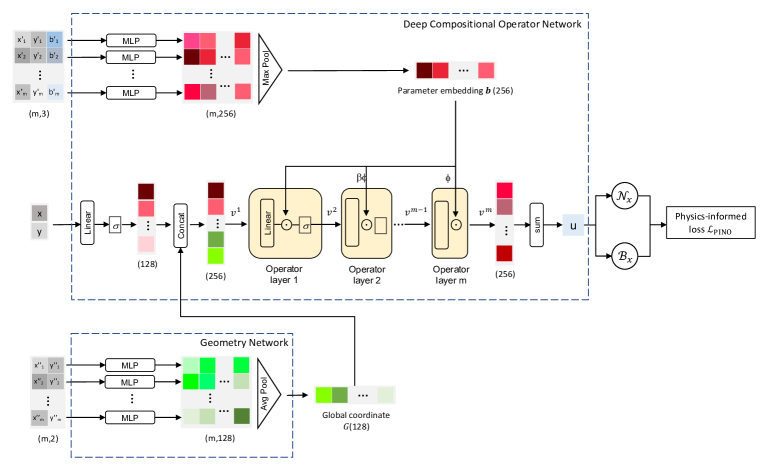
Figure 2: The architecture of the physics-informed Geometry aware Neural Operator is shown. The grey blocks represent the coordinates and the blue blocks represent the function values. The red blocks represent the hidden embeddings. The value of $b^{\prime}_{i}$ is the boundary condition value evaluated on $(x^{\prime}_{i},y^{\prime}_{i})$. The value of $u$ is the solution value evaluated on $(x,y)$. It should be noted that no activation function is included in the last operator layer.

3.3 Derivative approximation

Although our model utilizes a similar architecture to PI-PointNet for generating geometry embeddings and coupling global and local features, there are fundamental differences between our architecture and that of PI-PointNet. In the physics-informed training algorithm, we estimate the network parameters by minimizing the PDE residual. This residual in general involves spatial and temporal derivatives which means taking the derivative with respect to the input layer. Therefore, the backward propagation path for derivative calculation using auto differentiation plays a significant role in the quality of physics-informed training.

Figure 3 shows the computation graphs of PI-PointNet (top) and our model (bottom) for PDE solution in a two-dimensional domain. Solid arrows indicate the forward computation steps, and dashed arrows show the backward propagation steps for derivative calculation. If the two MLPs in our model are identical, it appears that our model and PI-PointNet would share the exact same computation path for PDE solution prediction. However, in our model, the computation of local (collocation point-based) features is independent from that for global features. This results in different computation paths for the derivatives of the model. For instance, in PI-PointNet, the first order derivative of $u_{j}$ with respect to coordinate $x_{j}$ is formulated by:

$$\frac{\partial u_{j}}{\partial x_{j}}=\frac{\partial u_{j}}{\partial H_{j}}\cdot\left[\frac{\partial H_{j}}{\partial h_{j}}\|\frac{\partial H_{j}}{\partial G}\frac{\partial G}{\partial h_{j}}\right]\cdot\frac{\partial h_{j}}{\partial x_{j}},$$ (21)

where $\|$ represents the operation of concatenation. However, the derivative approximation in our model architecture is simpler than Equation 21, which is formulated by:

$$\frac{\partial u_{j}}{\partial x_{j}}=\frac{\partial u_{j}}{\partial H_{j}}\cdot\frac{\partial H_{j}}{\partial h_{j}}\cdot\frac{\partial h_{j}}{\partial x_{j}}.$$ (22)

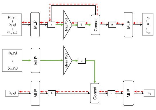
Figure 3: The differences between our model architecture and PI-PointNet are shown. The black solid arrows are forward computation path for PDE solution prediction, while the red dashed arrows are backward computation path for derivative calculation of the approximated function.

Comparing Equation 21 to Equation 22, it is evident that the differentiation process in our proposed architecture involves calculating only the derivatives of MLPs, whereas the PI-PointNet’s differentiation process also involves taking the derivative of the Max-pooling layer. Based on the Universal Approximation Theorem for neural networks Attali and Pagès (1997), an MLP can approximate any continuous function and its derivatives within certain error bounds. This is while automatic differentiation over the Max-pooling layer, negatively impacts the model’s performance. The numerical results presented in Section 4.3 will further show the differences in performance between these two backpropagation paths.

4 Numerical results

In this section, we numerically evaluate the accuracy of the proposed model for solving parametric differential equations. We compare our models with Physics-informed DCON (PI-DCON), Physics-informed PointNet (PI-PointNet). In order to add PDE parameter generalizability to PI-PointNet, we will also introduce a modified version of PI-PointNet, named PI-PointNet* (as explained in Section 4.1). This modified model, as an additional baseline model, offers a more fair comparison of effectiveness in generalization to variations in both PDE parameters and domain geometry.

In the numerical experiments, we use the following default settings unless mentioned otherwise. We use the hyperbolic tangent function (Tanh) Lau and Lim (2018) as our activation function to ensure the smoothness in high-order derivatives of the models. For PI-DCON and our model architecture, we use three operator layers of width 512. For the architecture of PI-PointNet and PI-PointNet*, we use three hidden layers of width 512. Adam is the default optimizer with the following default hyper-parameters: $\beta_{1}$ = 0.9 and $\beta_{2}$ = 0.999 Kingma and Ba (2014). Each model is trained on 70% of the sampled PDE parameters and validated on 10% of the sampled PDE parameters. Well-trained models predict the PDE solution for the remaining 20% of the sampled PDE parameters. There are two hyper-parameters used in model training: learning rate and coordinate sampling size ratio in each epoch for computing the PDE residual. We implemented grid search Bergstra and Bengio (2012) to obtain the best set of hyper-parameters and report the corresponding model performance. The possible values of learning rate are 0.001, 0.0005, 0.0002, and 0.0001, and the possible values of coordinate sampling size ratio are 0.3,0.2,0.1,0.05. Model training is performed on an NVIDIA P100 GPU using a batch size of 20. We collect the parameters of PDEs by Monte Carlo Simulation Mooney (1997) of stochastic processes Parzen (1999) and derive the solution of PDEs based on the Finite Element Method using Matlab Matlab (2012).

4.1 A modified PI-PointNet as a baseline

In its original form, PI-PointNet is not designed for generalization across different PDE parameters. Therefore, to create a baseline with this generalization capability, we have modified it to include a part which encodes PDE parameter information into the model inputs. In this modified architecture, called PI-PointNet*, if the function values of PDE parameters are available, they are concatenated with the coordinates of the collocation points as the model input. If not available, zeros are concatenated instead. This setup ensures that both the PDE parameters and the domain geometry are provided to the model, allowing the PDE solution to depend on both factors. Figure 4 shows the architecture of PI-PointNet* for the scenario where the only variable PDE parameter is the boundary conditions.

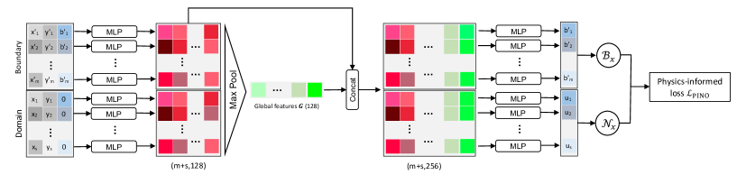
Figure 4: The architecture of the modified physics-informed PointNet (PI-PointNet*) is shown.

4.2 Experiment Setups

4.2.1 A Darcy flow problem

Let us consider a two-dimensional Darcy flow problem in a five-edge polygon. The steady state solution of the system is described by the following equation:

$$-\nabla(k(x,y)\nabla p(x,y)) =f(x,y),\quad(x,y)\in\Omega,$$ (23)

$$p(x,y) =g(x,y),\quad(x,y)\in\partial\Omega.$$

where $p(x,y)$ is the pressure, $k(x,y)$ is the permeability field, $f(x,y)$ is the source term, and $g(x,y)$ is the prescribed pressure on the domain boundaries $\partial\Omega$. Following the same setting as Lu et al. (2022), we consider $k(\bm{x})=1$ and $f(\bm{x})=10$. To create variable domain geometries, we consider an analytical expressions, where the coordinates of the five vertices of the polygon is varied. To do so, we first draw five random coordinates to be the center points for the five circles of radius of $0.25$ as shown in  5. These five center points are uniformly drawn on the perimeter of the circle, with the radius of $1$ centered at $(0,0)$. Inside each of the five circles, we will randomly generate one point to serve as a vertex of the polygon-shaped domain.

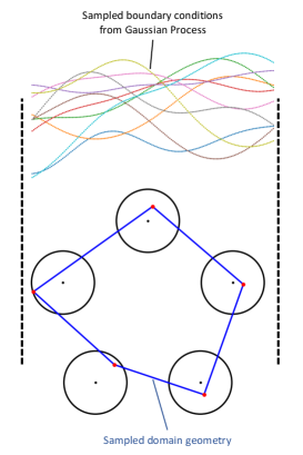
Figure 5: The boundary conditions in our Darcy flow experiment setting shown on a random geometry. The boundary conditions $g(\bm{x})$ are samples from a Gaussian process.

The boundary $\partial\Omega$ in this example is chosen to be the edges of the polygon, on which we impose the nonzero pressure function $g(x,y)$. The imposed pressure is assumed to follow a zero mean Gaussian process with a covariance kernel that is only dependent on the horizontal component of the distance, i.e.,

$$g(x,y) \sim\mathcal{GP}(0,K(x,x^{\prime})),$$ (24)

$$K(x,x^{\prime}) =\exp\left[-\frac{(x-x^{\prime})^{2}}{2l^{2}}\right],\quad l=1.$$

We employ the Gaussian process model of Eq. 24 to generate $N=1000$ different imposed pressure functions. Then, given each of these $N$ sampled functions, $\{g_{i}\}_{i=1}^{N}$, we solve the PDE using the Finite Element Method (FEM) Matlab (2012). Specifically, for the $i$-th realized domain $\Omega_{i}$ and BC function $g_{i}$, let $M_{i}$ be the number of discretization locations on $\partial\Omega_{i}$, and $\bm{X}_{\text{BC},i}$ be the coordinates of these locations, i.e.

$$\bm{X}_{\text{BC},i}=\{(x_{j}^{i},y_{j}^{i})\}_{j=1}^{M^{i}},$$ (25)

where $M^{i}$ is the size of the discretization generated for the $i$-th sampled geometry. We then collect all the boundary conditions information for the $i$-th geometry in $\bm{G}^{i}$, i.e.

$$\bm{G}_{i}=\{\bm{X}_{\text{BC},i},g_{i}(\bm{X}_{\text{BC},i})\},$$ (26)

where $g_{i}(\bm{X}_{\text{BC},i})$ is the $i$-th sampled BC function evaluated at the coordinates $\bm{X}_{\text{BC},i}$.

Given this setup, we seek to learn the nonlinear mapping $\mathcal{M}_{\text{Darcy}}$ that transforms a given boundary function $g(x,y)$ on $\partial\Omega$ to the pressure field $p(x,y)$ in the entire domain, i.e.,

$$\mathcal{M}_{\text{Darcy}}:g(x,y)\rightarrow p(x,y).$$ (27)

Specifically, for a 2D problem, the neural operator $p_{\theta}(x,y,\bm{G})$ is trained using the loss function

$$\mathcal{L}(\theta)=\mathcal{L}_{\text{PDE}}(\theta)+\alpha\mathcal{L}_{\text{BC}_{1}}(\theta),$$ (28)

where $\alpha$ is the weighing hyperparameters, set to be $\alpha=500$ to ensure similar orders of magnitude; $\mathcal{L}_{\text{PDE}}(\theta)$ and $\mathcal{L}_{\text{BC}}(\theta)$ are the PDE residual and the BC loss function, given by

$$\mathcal{L}_{\text{PDE}}(\theta) =\frac{1}{N}\sum_{i=1}^{N}\left[\frac{\partial^{2}p_{\theta}(x,y,\bm{G}_{i})}{\partial x^{2}}+\frac{\partial^{2}p_{\theta}(x,y,\bm{G}_{i})}{\partial y^{2}}+10\right]^{2}, (x,y)\in\Omega$$ (29)

$$\mathcal{L}_{\text{BC}}(\theta) =\frac{1}{N}\sum_{i=1}^{N}\left\{\frac{1}{M_{i}}\sum_{j=1}^{M_{i}}\left[p_{\theta}(x^{i}_{j},y^{i}_{j},\bm{G}_{i})-0\right]^{2}\right\}, (x^{i}_{j},y^{i}_{j})\in\bm{X}_{\text{BC},i}.$$

4.2.2 A 2D plate problem

In this example, we consider a more complex problem which involves a system of differential equations and a nonlinear mapping is to be learned between multiple parameter functions and multiple response functions. In particular, let us consider a solid mechanics problem for a two-dimensional plate with four holes. The static solution for the plate displacements is governed by the following system of partial differential equations

$$\frac{E}{1-\mu^{2}}\left[\frac{\partial^{2}u(x,y)}{\partial x^{2}}+\frac{(1-\mu)}{2}\frac{\partial^{2}u(x,y)}{\partial y^{2}}+\frac{(1+\mu)}{2}\frac{\partial^{2}v(x,y)}{\partial x\partial y}\right] =0,\quad(x,y)\in\Omega,$$ (30)

$$\frac{E}{1-\mu^{2}}\left[\frac{\partial^{2}v(x,y)}{\partial y^{2}}+\frac{(1-\mu)}{2}\frac{\partial^{2}v(x,y)}{\partial x^{2}}+\frac{(1+\mu)}{2}\frac{\partial^{2}u(x,y)}{\partial x\partial y}\right] =0,\quad(x,y)\in\Omega,$$

where $u$ and $v$ are the plate displacements in $x$ and $y$ directions, respectively, $E$ is the Young’s Modulus, and $\mu$ is the Poisson’s Ratio.

In this experiment, the plate is considered to be 20 mm $\times$ 20 mm, and the location and size of the bolts are variable. To generate variable geometries, we first consider four circles of radius of 1.5 centered at $(5,5)$, $(5,-5)$, $(-5,5)$, and $(-5,-5)$ respectively (shown by dashed lines in Figure 6). In each circle, we randomly select one point to be the center of a bolt hole. The radius of the holes are uniformly drawn from the range $[0.8,1.5]$. The edge of the holes are subjected to the “fixed" boundary condition (zero displacements). The left and right sides of the plate are subject to a prescribed imposed displacements (given as variable functions), while the top and bottom sides are assigned the “free" boundary conditions (zero strains).

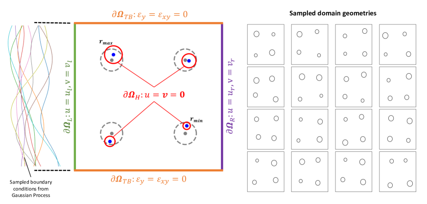
Figure 6: The boundary conditions of 2D Plate experiment, and 2D plates with largest and smallest bolt hole area are shown. The samples of Gaussian processes as the prescribed displacement on leftmost edges and rightmost edges are also shown. The dots on the curve are considered as the representation of the prescribed displacements.

The complete boundary conditions are shown in Figure  6, and are given by

$$u(x,y)=0,\quad v(x,y)=0,\quad(x,y)\in\partial\Omega_{\text{H}},$$ (31)

$$u(x,y)=u_{L}(x,y),\quad v(x,y)=v_{L}(x,y)\quad(x,y)\in\partial\Omega_{\text{L}},$$

$$u(x,y)=u_{R}(x,y),\quad v(x,y)=v_{R}(x,y)\quad(x,y)\in\partial\Omega_{\text{R}},$$

$$\frac{\partial v(x,y)}{\partial y}=0,\quad\frac{1}{2}\left[\frac{\partial u(x,y)}{\partial y}+\frac{\partial v(x,y)}{\partial x}\right]=0,\quad(x,y)\in\partial\Omega_{\text{TB}},$$

where the prescribed displacement functions $u_{L},v_{L},u_{R},v_{R}$ are the input functions to the operator. Similar to the previous example, these functions are considered to follow a Gaussian Process model. The covariance kernel is assumed to be dependent only on the vertical component of the distance, i.e.,

$$u_{l},v_{l},u_{R},v_{R} \sim\mathcal{GP}(1,K(y,y^{\prime})),$$ (32)

$$K(y,y^{\prime}) =\exp\left[-\frac{(y-y^{\prime})^{2}}{2l^{2}}\right],\quad l=5.$$

Similarly to the previous example, we draw $N=1000$ realizations of these functions, and obtain FEM solutions using meshes with different sizes. Figure 6 shows the scheme of the variable geometry generation and the boundary conditions settings. Some randomly generated geometries are also shown on the right. The boundary condition information on the left and right sides for the $i$-th realization is collected into the following four vectors

$$\bm{X}_{\text{BC}_{\text{TB}},i}=\{(x_{j}^{1,i},y_{j}^{1,i})\}_{j=1}^{M_{1,i}},$$ (33)

$$\bm{X}_{\text{BC}_{L},i}=\{(x_{j}^{2,i},y_{j}^{2,i})\}_{j=1}^{M_{2,i}},$$

$$\bm{X}_{\text{BC}_{R},i}=\{(x_{j}^{3,i},y_{j}^{3,i})\}_{j=1}^{M_{3,i}},$$

$$\bm{X}_{\text{BC}_{H},i}=\{(x_{j}^{4,i},y_{j}^{4,i})\}_{j=1}^{M_{4,i}},$$

where $\bm{X}_{\text{BC}_{1},i}$, $\bm{X}_{\text{BC}_{2},i}$, $\bm{X}_{\text{BC}_{3},i}$, $\bm{X}_{\text{BC}_{4},i}$ are the sets of boundary coordinates sampled on $\partial\Omega_{1}$, $\partial\Omega_{2}$, $\partial\Omega_{3}$, $\partial\Omega_{4}$, respectively. The discretized version of the input functions to the operator (sampled boundary values on the left and right sides) are then represented by the following matrices

$$\bm{G}_{L,i} =\{\bm{X}_{\text{BC}_{L},i},u_{L,i}(\bm{X}_{\text{BC}_{L},i}),v_{L,i}(\bm{X}_{\text{BC}_{L},i})\}$$ (34)

$$\bm{G}_{R,i} =\{\bm{X}_{\text{BC}_{R},i},u_{R,i}(\bm{X}_{\text{BC}_{R},i}),v_{R,i}(\bm{X}_{\text{BC}_{R},i})\}$$

Given this setup, we seek to learn the nonlinear mapping $\mathcal{M}_{\text{Plate}}$ that transforms the given boundary displacement functions $u_{L}(x,y),v_{L}(x,y),u_{R}(x,y),v_{R}(x,y)$ on $\partial\Omega_{2}$ and $\partial\Omega_{3}$ to the displacement field $u(x,y)$ and $v(x,y)$ in the entire domain, i.e.,

$$\mathcal{M}_{\text{Plate}}:[u_{L}(x,y),v_{L}(x,y),u_{R}(x,y),v_{R}(x,y)]\rightarrow[u(x,y),v(x,y)].$$ (35)

Based on these boundary condition settings, the training loss function $\mathcal{L}(\theta)$ for training of neural operators $u_{\theta}(x,y,\bm{G}_{L},\bm{G}_{R})$ and $v_{\theta}(x,y,\bm{G}_{L},\bm{G}_{R})$ is formulated as:

$$\mathcal{L}(\theta)=\alpha_{0}\mathcal{L}_{\text{PDE}}(\theta)+\alpha_{1}\mathcal{L}_{\text{BC}_{\text{TB}}}(\theta)+\alpha_{2}\mathcal{L}_{\text{BC}_{L}}(\theta)+\alpha_{3}\mathcal{L}_{\text{BC}_{R}}(\theta)+\alpha_{4}\mathcal{L}_{\text{BC}_{H}}(\theta),$$ (36)

where $\alpha_{0}$, $\alpha_{1}$, $\alpha_{2}$, $\alpha_{3}$, $\alpha_{4}$ are the trade-off coefficients, set to be $\alpha_{0}=0.00001,\alpha_{1}=\alpha_{2}=\alpha_{3}=\alpha_{4}=1$ to ensure similar orders of magnitude; and $\mathcal{L}_{\text{PDE}}(\theta)$ is the PDE residual given by

$$\mathcal{L}_{\text{PDE}}(\theta)=\frac{1}{N}\sum_{i=1}^{N} \left\{\frac{E}{1-\mu^{2}}\left(\frac{\partial^{2}u_{\theta}(x,y,\bm{G}_{L,i},\bm{G}_{R,i})}{\partial x^{2}}+\frac{\partial^{2}v_{\theta}(x,y,\bm{G}_{L,i},\bm{G}_{R,i})}{\partial y^{2}}\right)+\right.$$ (37)

$$\left.\frac{E}{2(1+\mu)}\left(\frac{\partial^{2}u_{\theta}(x,y,\bm{G}_{L,i},\bm{G}_{R,i})}{\partial y^{2}}+\frac{\partial^{2}v_{\theta}(x,y,\bm{G}_{L,i},\bm{G}_{R,i})}{\partial x^{2}}\right)+\right.$$

$$\left.\frac{E}{2(1-\mu)}\left(\frac{\partial^{2}v_{\theta}(x,y,\bm{G}_{L,i},\bm{G}_{R,i})}{\partial x\partial y}+\frac{\partial^{2}u_{\theta}(x,y,\bm{G}_{L,i},\bm{G}_{R,i})}{\partial x\partial y}\right)\right\},\quad(x,y)\in\Omega.$$

The BC loss terms $\mathcal{L}_{\text{BC}_{\text{TB}}}(\theta)$, $\mathcal{L}_{\text{BC}_{L}}(\theta)$, $\mathcal{L}_{\text{BC}_{R}}(\theta)$, $\mathcal{L}_{\text{BC}_{H}}(\theta)$ are given by

$$\mathcal{L}_{\text{BC}_{\text{TB}}}(\theta)=\frac{1}{N}\sum_{i=1}^{N} \left\{\frac{1}{M_{1,i}}\sum_{j=1}^{M_{1,i}}\left[u_{\theta}(x_{j}^{i},y_{j}^{i},\bm{G}_{L,i},\bm{G}_{R,i})-0\right]^{2}+\left[v_{\theta}(x_{j}^{i},y_{j}^{i},\bm{G}_{L,i},\bm{G}_{R,i})-0\right]^{2}\right\},\quad(x_{j}^{i},y_{j}^{i})\in\bm{X}_{\text{BC}_{\text{TB}},i},$$ (38)

$$\mathcal{L}_{\text{BC}_{L}}(\theta)=\frac{1}{N}\sum_{i=1}^{N} \left\{\frac{1}{M_{2,i}}\sum_{j=1}^{M_{2,i}}\left[u_{\theta}(x_{j}^{i},y_{j}^{i},\bm{G}_{L,i},\bm{G}_{R,i})-u_{L,i}(x_{j}^{i},y_{j}^{i})\right]^{2}+\left[v_{\theta}(x_{j}^{i},y_{j}^{i},\bm{G}_{L,i},\bm{G}_{R,i})-v_{L,i}(x_{j}^{i},y_{j}^{i})\right]^{2}\right\},$$

$$(x_{j}^{i},y_{j}^{i})\in\bm{X}_{\text{BC}_{L},i},$$

$$\mathcal{L}_{\text{BC}_{R}}(\theta)=\frac{1}{N}\sum_{i=1}^{N} \left\{\frac{1}{M_{3,i}}\sum_{j=1}^{M_{3,i}}\left[u_{\theta}(x_{j}^{i},y_{j}^{i},\bm{G}_{L,i},\bm{G}_{R,i})-u_{R,i}(x_{j}^{i},y_{j}^{i})\right]^{2}+\left[v_{\theta}(x_{j}^{i},y_{j}^{i},\bm{G}_{L,i},\bm{G}_{R,i})-v_{R,i}(x_{j}^{i},y_{j}^{i})\right]^{2}\right\},$$

$$(x_{j}^{i},y_{j}^{i})\in\bm{X}_{\text{BC}_{R},i},$$

$$\mathcal{L}_{\text{BC}_{H}}(\theta)=\frac{1}{N}\sum_{i=1}^{N} \left\{\frac{1}{M_{4,i}}\sum_{j=1}^{M_{4,i}}\left[\frac{\partial v_{\theta}(x_{j}^{i},y_{j}^{i},\bm{G}_{L,i},\bm{G}_{R,i})}{\partial y_{j}^{i}}-0\right]^{2}+\right.$$

$$\left.\left[\frac{1}{2}\left(\frac{\partial u_{\theta}(x_{j}^{i},y_{j}^{i},\bm{G}_{L,i},\bm{G}_{R,i})}{\partial y_{j}^{i}}+\frac{\partial v_{\theta}(x_{j}^{i},y_{j}^{i},\bm{G}_{L,i},\bm{G}_{R,i})}{\partial x_{j}^{i}}\right)-0\right]^{2}\right\},\quad(x_{j}^{i},y_{j}^{i})\in\bm{X}_{\text{BC}_{H},i}.$$

4.3 Main results

For both the Darcy flow problem and the 2D Plate problem, we will generate two datasets: one with varying geometry only, and the other one with both varying PDE parameters and varying geometry. The first dataset is used to only investigate geometry generalization and compare the performance of our proposed model with that of PI-PointNet. The second dataset is utilized to evaluate the parameter and geometry generalization abilities of our proposed model with PI-DCON and PI-PointNet*. It should be noted that for the 2D plate dataset, to properly discretize the boundary around the small holes, we employ a higher resolution compared to the Darcy problem. Typically, the meshes in the Darcy flow dataset contain approximately 1,000 nodes, whereas the meshes in 2D plate dataset has about 30,000 nodes. We use relative $L_{2}$ error Heydari and Bagheri (2012) as our error measure computed by:

$$L_{2}=\frac{\|\bm{u}_{\text{pred}}-\bm{u}_{\text{fem}}\|_{2}}{\|u_{\text{fem}}\|_{2}},$$ (39)

where $u_{\text{pred}}$ refers to a vector of neural network predictions at all the collocation points, and $u_{\text{fem}}$ is the corresponding FEM solution vector. We present the average error calculated across the entire test dataset, along with the standard deviation of the relative errors to demonstrate the model stability.

Table LABEL:table.PI_com_only_geo shows the results for the case where only geometry generalization is compared with PI-PointNet. As can be seen, our model achieved 39.1% accuracy improvement for the Darcy flow problem and 75.0% accuracy improvement for the 2D Plate problem. Figure 7, in more details, compare the two models, and show the our method in all the geometry samples offers smaller error compared to PI-PointNet.

Table 2: Accuracy and efficiency comparison between PI-GANO and PI-PointNet for the dataset of only geometry variation.

Dataset	Mean of relative error		Standard deviation of relative error		Training time (minutes)
	PI-PointNet	PI-GANO	PI-PointNet	PI-GANO	PI-PointNet	PI-GANO
Darcy flow	11.30%	6.70%	3.52%	2.09%	32	18
2D Plate	25.72%	6.41%	10.13%	2.19%	265	57

(a) Darcy flow

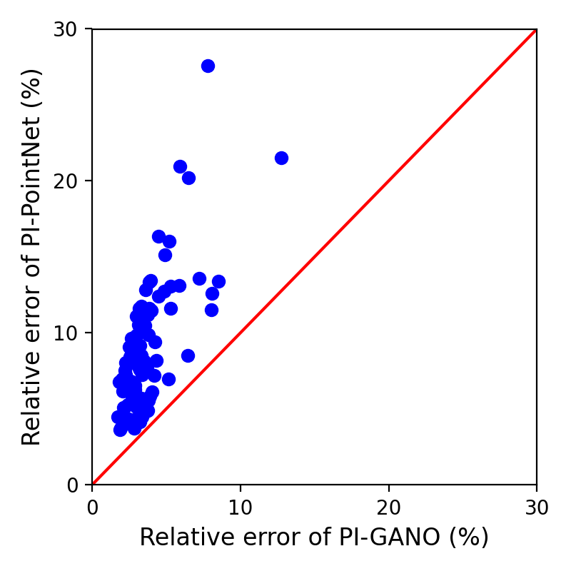
(b) 2D plate

Figure 7: Comparison between PI-GANO and PI-PointNet on the Darcy flow and 2D plate problems. It can be seen that in all the cases PI-GANO offers the smaller errors.

Comparing the training times of the two models, we demonstrate that our method surpasses PI-PointNet in terms of efficiency, especially when handling fine meshes, noting the results for the 2D plate problem. In physics-informed training, the computation of PDE residuals is required in each iteration. In our proposed model, we can sample a small subset of the collocation points, in the trunk net, for the approximation calculation of loss and an efficient update of the model parameters. This is because the trunk net, which approximate the solution at a given point, is chosen to be separate from the geometry encoder. In contrast, PI-PointNet can only handle the entire point cloud representing the entire domain. Therefore, stochastic gradient descent algorithm with a small minibatch size cannot work for this model architecture. As a result, we observe a significantly reduced training time for our model when dealing with fine meshes. To visually compare our method with PI-PointNet, the best and worst-case predictions are presented in Table 3.

Table 3: Comparison between the performance of PI-GANO and PI-PointNet. Out of all realizations of boundary conditions, the ones that causes best and worst performances of each model are shown.

		Ground Truth	PI-PointNet		PI-GANO
			Prediction	Absolute Error	Prediction	Absolute Error
Darcy flow	PI-PointNet Best case
	PI-GANO Best case
	PI-PointNet Worst case
	PI-GANO Worst case
2D Plate	PI-PointNet Best case
	PI-GANO Best case
	PI-PointNet Worst case
	PI-GANO Worst case

For cases where both PDE parameters and geometries vary, we compare our method with PI-DCON and PI-PointNet* in Table LABEL:table.PI_com. It can be seen that the PI-PointNet* struggles to achieve satisfactory accuracy, underscoring the challenge of developing a model capable of generalizing to varying PDE parameters and geometries. Our proposed model demonstrated highest accuracy in addressing both the Darcy flow problem and the 2D Plate problem. Compared to PI-DCON, our model achieved a 60% accuracy improvement for the Darcy flow problem and a 50% accuracy improvement for the 2D Plate problem, illustrating the effectiveness of the geometry encoder in our model. Figure 8 shows more detailed comparison between the errors calculated for each testing samples, and underlines the superiority of PI-GANO in all the test cases.

Table 4: Accuracy comparison between PI-GANO and PI-DCON.

	Mean of relative error			Standard deviation of relative error
Dataset	PI-PointNet*	PI-DCON	PI-GANO	PI-PointNet*	PI-DCON	PI-GANO
Darcy flow	64.3%	13.50%	8.40%	24.7%	5.88%	2.53%
2D Plate	74.3%	14.06%	7.12%	27.8%	4.81%	2.82%

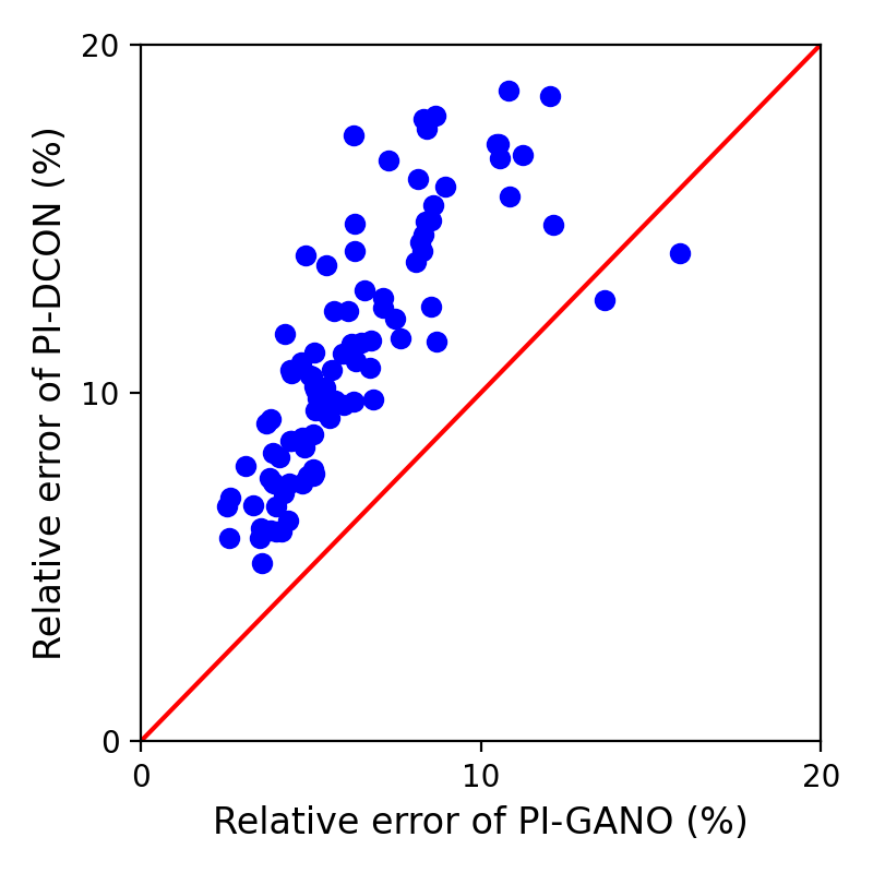
(a) Darcy flow

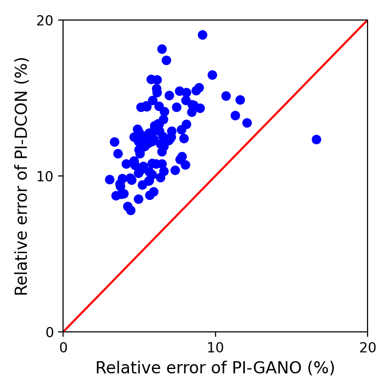
(b) 2D plate

Figure 8: Comparison between PI-GANO and PI-DCON on the Darcy flow and 2D plate problems. It can be seen that in all the cases PI-GANO offers the smaller errors.

To better illustrate the performance of our model, Table 5 shows the predictions from PI-DCON and PI-GANO and their errors compared to the FEM prediction, for various best and worst-case scenarios. Overall, our model shows higher accuracy maintaining acceptable performance even in its worst cases. Furthermore, the relatively small performance gaps between the worst and best cases underscore the robustness of our model.

Table 5: Comparison between the performance of PI-GANO and PI-DCON. Out of all realizations of boundary conditions, the ones that causes best and worst performances of each model are shown.

		Ground Truth	PI-DCON		PI-GANO
			Prediction	Absolute Error	Prediction	Absolute Error
Darcy flow	PI-DCON Best case
	PI-GANO Best case
	PI-DCON Worst case
	PI-GANO Worst case
2D Plate	PI-DCON Best case
	PI-GANO Best case
	PI-DCON Worst case
	PI-GANO Worst case

4.4 Ablation study: Different geometry embeddings

In previous experiments, we used the collocation points on the boundary to infer important features of domain geometry. These collocation points can be collected from different parts of the domain. In particular, in this section, we study four different ways to do so: (1) collecting collocation points on segments of the boundary that vary, (2) collecting collocation points on all boundary segments, (3) collecting collocation points in the entire domain. As an additional case, we also consider using directly the parametric representation of the geometry, which in our examples are available.

The parametric geometry representation of the Darcy flow problem consists of the coordinates of the five points that form the polygon, i.e. a total of 10 coordinates. Similarly, for the 2D plate problem, the parametric geometry representation contains the locations and sizes of the four holes, i.e. a total of 12 parameters. For cases where the parametric representation is used, the geometry encoder will be simply a multi-layer perceptron.

As shown in Table LABEL:table.different_geometry_embeddings, the highest model accuracy is achieved when using collocation points from varying boundaries. Although using all collocation points provides the most comprehensive information about the domain geometry, this approach results in the poorest model performance. This can be due to the fact that many interior point locations are common across different geometries, rendering them redundant in capturing distinct geometric features leading to deterioration in effective geometry encoding. Furthermore, when comparing model performance using points from varying boundaries and parametric representations, the use of varying boundary points leads to 1.7% accuracy improvement for the Darcy flow problem and 20% improvement for the 2D Plate problem, indicating that parametric representations is not necessarily always the most effective approach.

Table 6: Mean of relative error of different geometry embedding usage.

Geometry input data	Interior and boundary points	Boundary points (fixed and variable)	Parameters of parametric representation	Boundary points (variable only)
Darcy flow	11.1%	/	8.56%	8.40%
2D plate	21.17%	14.81%	9.02%	7.21%

In our proposed architecture, we used concatenation to combine the geometry embedding with the local coordinate embedding. Here, we study the performance of the model when these two embeddings are integrated using other forms. In particular, we consider the following three cases

$$\text{Multiplication}: \quad\bm{H}_{j}^{i}=\bm{h}^{i}_{j}\odot\bm{G}^{i},$$ (40)

$$\text{Addition}: \quad\bm{H}_{j}^{i}=\bm{h}^{i}_{j}+\bm{G}^{i},$$ (41)

$$\text{Concatenation}: \quad\bm{H}_{j}^{i}=[\bm{h}^{i}_{j}\|\bm{G}^{i}],$$ (42)

where $\bm{G}^{i}$ is the global feature of the $i$-th geometry, $\bm{h}^{i}_{j}$ is the local hidden embedding of the $j$-th coordinate in the $i$-th geometry, and $\bm{H}^{i}_{j}$ is the global hidden embedding of the $j$-th coordinate in the $i$-th geometry. To generate the results, we only use collocation points on the varying boundary, which was shown earlier to be the best approach. As can be seen in Table LABEL:table.different_geometry_embed_method, concatenation offers the highest accuracy.

Table 7: Mean of relative error of different geometry embedding methods.

Problem	Operations
	Multiplication	Addition	Concatenation
Darcy flow	11.13 %	10.90%	8.40%
2D plate	15.17%	13.81%	7.21%

4.5 Generalization for large geometry variation

In this section, we further explore the geometry generalization using a dataset with significantly higher geometry variation. This dataset is created under the same settings as those described in Section 4.2.2, with the exception that the holes can be of any radius and they can be placed anywhere on the plate, as long as they do not protrude beyond the outer edges. Overlapping holes are also allowed in this data generation, merely to create a more challenging generalization test. To ensure comprehensive coverage of the highly variable geometric distribution, we generate 5,000 different geometry samples. The size ratio of the training , validation and testing datasets are 70%, 10%, and 20%, respectively.

As indicated in Table LABEL:table.PI_com_high_variation, our proposed model achieves approximately a 70% accuracy improvement on this challenging dataset, underscoring its robustness in handling highly varying geometries. By visually comparing the model’s performances, Table LABEL:table.PI_com_high_variation shows that PI-GANO can offer more accurate predictions for various best and worst-case scenarios.

Table 8: Accuracy comparison between PI-GANO and PI-DCON for the dataset of high geometry variation.

Model	Mean of relative error	Standard deviation of relative error
PI-DCON	23.72%	10.91%
PI-GANO	7.29%	3.22%

Table 9: Comparison between the performance of PI-DCON and PI-DeepONet. Out of all realizations of boundary conditions, the ones that causes best and worst performances of each model are shown.

		Ground Truth	PI-DCON		PI-GANO
			Prediction	Absolute Error	Prediction	Absolute Error
2D Plate	PI-DCON Best case
	PI-GANO Best case
	PI-DCON Worst case
	PI-GANO Worst case

4.6 Comparison with data-driven neural operators

In this section, we evaluate the efficiency and accuracy of our proposed physics-informed model compared to the data-driven (supervised) versions of DCON and GANO architectures. We use the same dataset of 500 samples, as in our previous experiments, with 70% allocated for training, 10% for validation, and 20% for testing. The total time for FEM data generation is estimated based on 350 FEM computations. We report the accuracy of the two data-driven models in Table LABEL:table.data_driven_com, where the proposed GANO architecture offers superior accuracy over DCON. We also present the best model performance achieved versus the total time of building the model in Figure 9. For the data-driven models, the total time includes the data generation and training times. It can be seen that for the Darcy flow problem, PI-GANO reaches a convergence accuracy comparable to that of data-driven GANO and DCON, while requiring less time to achieve this accuracy level. This underscores the efficiency benefits of using physics-informed training to develop neural operators. Additionally, data-driven GANO and data-driven DCON exhibit similar prediction accuracy levels. We attribute this to the fact that the variable PDE parameter, which are the boundary conditions, in the Darcy flow problem, are imposed on the entire exterior boundary of the domain. This means that the PDE parameter input also inherently contains geometry information about the entire geometry. Therefore, the addition of a separate geometry encoder does not significantly enhance the model performance.

On the other hand, for the 2D plate problem, data-driven GANO achieves over a 28% accuracy improvement compared to data-driven DCON. This shows it is important to include a separate geometry encoder, because the variable parameters in this problem are only imposed on a subset of boundary segments, which do not fully characterize the entire domain. Furthermore, it can be seen in this figure that our proposed PI-GANO outperforms the data-driven version of GANO, highlighting the potential of physics-informed training to offer efficiency and also to enhance prediction accuracy when the same model architecture is used.

We also observe that, in the 2D plate problem, the best model prediction accuracy of the physics-informed models does not always decrease with more training epochs. Instead, it may remains unchanged during parts of the training process. This phenomenon can be attributed to the small size of the collocation point sampling used for PDE residual computation to handle meshes of high resolutions. Using a small set of points for PDE residual computation can cause the model to overly focus on the accuracy of a small region in the domain, at the expense of overall approximation accuracy across the entire domain. This issue highlights the need for more advanced physics-informed training algorithms to enhance the training of neural operators

Table 10: Accuracy comparison between data-driven DCON and data-driven GANO.

Dataset	Mean of relative error		Standard deviation of relative error
	Data-driven DCON	Data-driven GANO	Data-driven DCON	Data-driven GANO
Darcy flow	8.21%	8.00%	3.27%	2.93%
2D plate	13.5%	9.01%	4.56%	3.17%

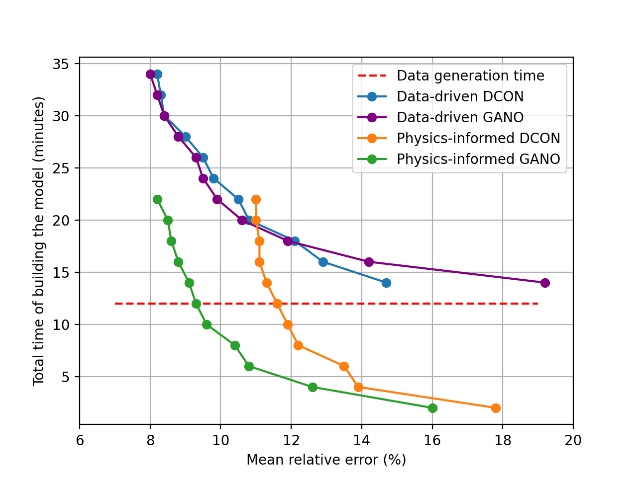
(a) Darcy flow problem

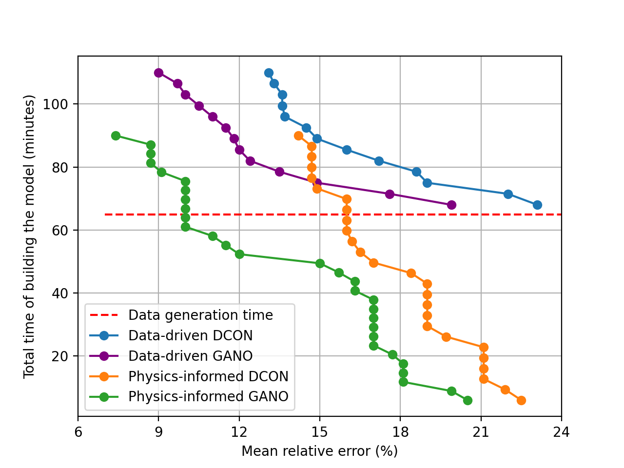
(b) 2D plate problem

Figure 9: Comparison between the total time needed to train different neural operators. For data-driven method, this time also includes the time needed to generate the training (FE simulation) data.

5 Conclusion

In this study, we introduced PI-GANO, a physics-informed neural operator inspired by PI-PointNet and PI-DCON, marking the first attempt to construct a neural operator capable of generalizing to both variable PDE parameters and variable domain geometries without the need for FEM training data or a regular meshing of domains. Our results demonstrate that PI-GANO can effectively predict PDE solutions for variable boundary conditions and domain geometries. Moreover, comparing the proposed PI-GANO with the data-driven version of our proposed architecture, we showed the potential of physics-informed training to offer efficiency and accuracy benefits in developing neural operators.

Despite these advancements, our approach has its limitations. Primarily, our evaluation focuses solely on the model’s capability to compute steady-state solutions. Further research is needed to adapt PI-GANO to handle dynamic responses, thereby enabling it to address time-dependent PDEs. Additionally, we observed instability in physics-informed training, which leads to requiring more training epochs to identify optimal model parameters. To address this, we seek to adopt a more intelligent collocation point sampling strategy, importance sampling Nabian et al. (2021), for physics-informed training. Furthermore, while our model currently relies on a basic multi-layer perceptron structure, incorporating more sophisticated architectures, such as attention mechanisms Vaswani et al. (2017), may further enhance its performance.

References

- Almasri et al. [2024] Waad Almasri, Dimitri Bettebghor, Faouzi Adjed, Florence Danglade, and Fakhreddine Ababsa. Geometrically-driven generation of mechanical designs through deep convolutional gans. Engineering Optimization, 56(1):18–35, 2024.
- Attali and Pagès [1997] Jean-Gabriel Attali and Gilles Pagès. Approximations of functions by a multilayer perceptron: a new approach. Neural networks, 10(6):1069–1081, 1997.
- Bergstra and Bengio [2012] James Bergstra and Yoshua Bengio. Random search for hyper-parameter optimization. Journal of machine learning research, 13(2), 2012.
- Dhatt et al. [2012] Gouri Dhatt, Emmanuel Lefrançois, and Gilbert Touzot. Finite element method. John Wiley & Sons, 2012.
- Gholamalinezhad and Khosravi [2020] Hossein Gholamalinezhad and Hossein Khosravi. Pooling methods in deep neural networks, a review. arXiv preprint arXiv:2009.07485, 2020.
- Hao et al. [2023] Zhongkai Hao, Zhengyi Wang, Hang Su, Chengyang Ying, Yinpeng Dong, Songming Liu, Ze Cheng, Jian Song, and Jun Zhu. Gnot: A general neural operator transformer for operator learning. In International Conference on Machine Learning, pages 12556–12569. PMLR, 2023.
- Hemmasian and Farimani [2024] AmirPouya Hemmasian and Amir Barati Farimani. Multi-scale time-stepping of partial differential equations with transformers. Computer Methods in Applied Mechanics and Engineering, 426:116983, 2024.
- Heydari and Bagheri [2012] Pooneh Heydari and Mohammad S Bagheri. Error analysis: Sources of l2 learners’ errors. Theory and practice in language studies, 2(8):1583–1589, 2012.
- Kashefi and Mukerji [2022] Ali Kashefi and Tapan Mukerji. Physics-informed pointnet: A deep learning solver for steady-state incompressible flows and thermal fields on multiple sets of irregular geometries. Journal of Computational Physics, 468:111510, 2022.
- Kingma and Ba [2014] Diederik P. Kingma and Jimmy Ba. Adam: A method for stochastic optimization, 2014. URL https://arxiv.org/abs/1412.6980.
- Kovachki et al. [2021] Nikola Kovachki, Zongyi Li, Burigede Liu, Kamyar Azizzadenesheli, Kaushik Bhattacharya, Andrew Stuart, and Anima Anandkumar. Neural operator: Learning maps between function spaces. arXiv preprint arXiv:2108.08481, 2021.
- Lau and Lim [2018] Mian Mian Lau and King Hann Lim. Review of adaptive activation function in deep neural network. In 2018 IEEE-EMBS Conference on Biomedical Engineering and Sciences (IECBES), pages 686–690. IEEE, 2018.
- Lee and Oh [2024] Seungjun Lee and Taeil Oh. Inducing point operator transformer: A flexible and scalable architecture for solving pdes. In Proceedings of the AAAI Conference on Artificial Intelligence, volume 38, pages 153–161, 2024.
- Li et al. [2020a] Zongyi Li, Nikola Kovachki, Kamyar Azizzadenesheli, Burigede Liu, Kaushik Bhattacharya, Andrew Stuart, and Anima Anandkumar. Fourier neural operator for parametric partial differential equations. arXiv preprint arXiv:2010.08895, 2020a.
- Li et al. [2020b] Zongyi Li, Nikola Kovachki, Kamyar Azizzadenesheli, Burigede Liu, Kaushik Bhattacharya, Andrew Stuart, and Anima Anandkumar. Neural operator: Graph kernel network for partial differential equations. arXiv preprint arXiv:2003.03485, 2020b.
- Li et al. [2021] Zongyi Li, Hongkai Zheng, Nikola Kovachki, David Jin, Haoxuan Chen, Burigede Liu, Kamyar Azizzadenesheli, and Anima Anandkumar. Physics-informed neural operator for learning partial differential equations. arXiv preprint arXiv:2111.03794, 2021.
- Li et al. [2023] Zongyi Li, Daniel Zhengyu Huang, Burigede Liu, and Anima Anandkumar. Fourier neural operator with learned deformations for pdes on general geometries. Journal of Machine Learning Research, 24(388):1–26, 2023.
- Li et al. [2024] Zongyi Li, Nikola Kovachki, Chris Choy, Boyi Li, Jean Kossaifi, Shourya Otta, Mohammad Amin Nabian, Maximilian Stadler, Christian Hundt, Kamyar Azizzadenesheli, et al. Geometry-informed neural operator for large-scale 3d pdes. Advances in Neural Information Processing Systems, 36, 2024.
- Lu et al. [2021] Lu Lu, Pengzhan Jin, Guofei Pang, Zhongqiang Zhang, and George Em Karniadakis. Learning nonlinear operators via deeponet based on the universal approximation theorem of operators. Nature Machine Intelligence, 3(3):218–229, March 2021. ISSN 2522-5839. doi:10.1038/s42256-021-00302-5. URL http://dx.doi.org/10.1038/s42256-021-00302-5.
- Lu et al. [2022] Lu Lu, Xuhui Meng, Shengze Cai, Zhiping Mao, Somdatta Goswami, Zhongqiang Zhang, and George Em Karniadakis. A comprehensive and fair comparison of two neural operators (with practical extensions) based on fair data. Computer Methods in Applied Mechanics and Engineering, 393:114778, 2022.
- Matlab [2012] Starting Matlab. Matlab. The MathWorks, Natick, MA, 2012.
- Mooney [1997] Christopher Z Mooney. Monte carlo simulation. Sage, 1997.
- Nabian et al. [2021] Mohammad Amin Nabian, Rini Jasmine Gladstone, and Hadi Meidani. Efficient training of physics-informed neural networks via importance sampling. Computer-Aided Civil and Infrastructure Engineering, 36(8):962–977, 2021.
- Navaneeth et al. [2024] N Navaneeth, Tapas Tripura, and Souvik Chakraborty. Physics informed wno. Computer Methods in Applied Mechanics and Engineering, 418:116546, 2024.
- Parzen [1999] Emanuel Parzen. Stochastic processes. SIAM, 1999.
- Raissi et al. [2019] Maziar Raissi, Paris Perdikaris, and George E Karniadakis. Physics-informed neural networks: A deep learning framework for solving forward and inverse problems involving nonlinear partial differential equations. Journal of Computational physics, 378:686–707, 2019.
- Tripura and Chakraborty [2022] Tapas Tripura and Souvik Chakraborty. Wavelet neural operator: a neural operator for parametric partial differential equations. arXiv preprint arXiv:2205.02191, 2022.
- Van Merriënboer et al. [2018] Bart Van Merriënboer, Olivier Breuleux, Arnaud Bergeron, and Pascal Lamblin. Automatic differentiation in ml: Where we are and where we should be going. Advances in neural information processing systems, 31, 2018.
- Vaswani et al. [2017] Ashish Vaswani, Noam Shazeer, Niki Parmar, Jakob Uszkoreit, Llion Jones, Aidan N Gomez, Łukasz Kaiser, and Illia Polosukhin. Attention is all you need. Advances in neural information processing systems, 30, 2017.
- Wang et al. [2024] Chu Wang, Jinhong Wu, Yanzhi Wang, Zhijian Zha, and Qi Zhou. Mpipn: A multi physics-informed pointnet for solving parametric acoustic-structure systems. arXiv preprint arXiv:2403.01132, 2024.
- Wang et al. [2021] Sifan Wang, Hanwen Wang, and Paris Perdikaris. Learning the solution operator of parametric partial differential equations with physics-informed deeponets. Science advances, 7(40):eabi8605, 2021.
- Wu et al. [2024] Haixu Wu, Huakun Luo, Haowen Wang, Jianmin Wang, and Mingsheng Long. Transolver: A fast transformer solver for pdes on general geometries. arXiv preprint arXiv:2402.02366, 2024.
- Zhao et al. [2024] Zhiwei Zhao, Changqing Liu, Yingguang Li, Zhibin Chen, and Xu Liu. Diffeomorphism neural operator for various domains and parameters of partial differential equations. arXiv preprint arXiv:2402.12475, 2024.
- Zhong and Meidani [2024] Weiheng Zhong and Hadi Meidani. Physics-informed mesh-independent deep compositional operator network, 2024.