On the two-dimensional harmonic oscillator with an electric field confined to a circular box

Abstract

We revisit the quantum-mechanical two-dimensional harmonic oscillator with an electric field confined to a circular box of impenetrable walls. In order to obtain the energy spectrum we resort to the Rayleigh-Ritz method with polynomial and Gaussian basis sets. We compare present results with those derived recently by other authors. We discuss the limits of large and small box radius and also do some calculations with perturbation theory.

1 Introduction

In a paper published recently Cruz et al[1] studied a model for an electron confined to a circle of radius $r_{0}$ under the effect of a harmonic interaction and a uniform electric field. They solved the Schrödinger equation by means of the linear variational method (commonly known as the Rayleigh-Rith method (RRM)[2, 3]) and studied the effect of the box size and the magnitude of the electric field on the Shannon entropy and Fisher information for some of the lowest states of the system.

In their calculation Cruz et al resorted to an incomplete trial function that is a linear combination of states sharing the same radial part. Since there are no other results that may be chosen as benchmark it was not possible to estimate the accuracy of those variational results. In this paper we repeat the calculation using a suitable basis set. Since the RRM yields increasingly accurate upper bounds to the all eigenvalues of the problem[4, 5] we can easily estimate the accuracy of the results of Cruz et al.

2 Two-dimensional harmonic oscillator confined to a circle with a constant electric field

In what follows we outline some general features of the Schrödinger equation for the model as well as the earlier calculation carried out by Cruz et al[1].

2.1 Some general features of the eigenvalue equation

The problem discussed by Cruz et al is given by the Hamiltonian operator

$$H=-\frac{\hbar^{2}}{2m}\nabla^{2}+\frac{k}{2}r^{2}+efx+V_{c}(r),$$ (1)

where $m$ is the electron mass, $e$ is the electron charge, $k$ is the oscillator force constant, $f$ is the magnitude of the electric field and $V_{c}(r)$ is a confining potential given by

$$V_{c}(r)=\left\{\begin{array}[]{l}0\mathrm{\ if\;}0\leq r<r_{0}\\ \infty\;\mathrm{if\;}r\geq r_{0}\end{array}\right.,$$ (2)

that forces the boundary condition $\psi(x,y)=0$ for all $r=\sqrt{x^{2}+y^{2}}\geq r_{0}$.

2.2 Dimensionless equations

Before discussing the solution of the Schrödinger equation with the Hamiltonian operator (1) we briefly outline some relevant features of the model. To begin with, we consider the transformation $(x,y)=(L\tilde{x},L\tilde{y})$, $\nabla^{2}=L^{-2}\tilde{\nabla}^{2}$, where $L$ is an arbitrary unit of length and $(\tilde{x},\tilde{y})$ are dimensionless cartesian coordinates. In this way we derive the dimensionless Hamiltonian operator[6] (we omit the confining potential from now on)

$$\tilde{H}=\frac{mL^{2}}{\hbar^{2}}H=-\frac{1}{2}\tilde{\nabla}^{2}+\frac{mkL^{4}}{2\hbar^{2}}\tilde{r}^{2}+\frac{mefL^{3}}{\hbar^{2}}\tilde{x}.$$ (3)

The boundary condition now becomes $\tilde{\psi}(\tilde{x},\tilde{y})=0$ for all $\tilde{r}\geq\tilde{r}_{0}$, $\tilde{r}=r/L$, $\tilde{r}_{0}=r_{0}/L$.

We first consider the case $L=r_{0}$ that leads to

$$\tilde{H}=\frac{mr_{0}^{2}}{\hbar^{2}}H=-\frac{1}{2}\tilde{\nabla}^{2}+\frac{mkr_{0}^{4}}{2\hbar^{2}}\tilde{r}^{2}+\frac{mefr_{0}^{3}}{\hbar^{2}}\tilde{x},$$ (4)

from which it follows that

$$\lim\limits_{r_{0}\rightarrow 0}\tilde{H}=-\frac{1}{2}\tilde{\nabla}^{2}.$$ (5)

That is to say, when $r_{0}\rightarrow 0$ we obtain the model of a particle in a circular box with radius $\tilde{r}_{0}=1$. We will come back to this issue later on.

Cruz et al chose $L=\sqrt{\hbar/\sqrt{mk}}=\sqrt{\hbar/m\omega}$, where $\omega=\sqrt{k/m}$, so that

$$\tilde{H}=\frac{H}{\hbar\omega}=-\frac{1}{2}\tilde{\nabla}^{2}+\frac{1}{2}\tilde{r}^{2}+\lambda\tilde{x},\;\lambda=\frac{mefL^{3}}{\hbar^{2}}.$$ (6)

Throughout this paper we will use this form of the dimensionless Hamiltonian operator and omit the tilde on the dimensionless variables.

2.3 Earlier calculations

According to the results of the preceding subsection the dimensionless Hamiltonian operator for this model can be written as

$$H=-\frac{1}{2}\nabla^{2}+\frac{1}{2}r^{2}+\lambda r\cos(\phi),$$ (7)

where $r=\sqrt{x^{2}+y^{2}}$ and $0\leq\phi<2\pi$. The eigenfunctions $\psi(r,\phi)$ satisfy the boundary condition $\psi(r_{0},\phi)=0$.

Cruz et al first solved the eigenvalue equation for $\lambda=0$ and obtained the eigenfunctions in polar coordinates $\psi_{nm}^{(0)}\left(r,\phi\right)=R_{nm}(r)\frac{e^{im\phi}}{\sqrt{2\pi}}$, where $n=0,1,\ldots$ and $m=0,\pm 1,\pm 2,\ldots$ are the radial and magnetic quantum numbers, respectively. With such solutions they proposed trial variational functions of the form

$$\Psi(r,\phi)=\sum_{m=-M}^{M}c_{m}\psi_{nm}^{(0)}(r,\phi),$$ (8)

where $\psi_{nm}^{(0)}$ are the eigenfunctions of the $2D$ confined harmonic oscillator[1, 7]. It is clear that the general trial function should be

$$\Psi(r,\phi)=\sum_{n=0}^{N}\sum_{m=-M}^{M}c_{nm}\psi_{nm}^{(0)}(r,\phi),$$ (9)

because the term $\lambda r\cos(\phi)$ clearly couples states with different values of $n$. The latter approach requires the calculation of integrals of the form

$$\int_{0}^{r_{0}}R_{nm}(r)rR_{n^{\prime}m^{\prime}}(r)r\,dr,$$ (10)

that we can avoid if we choose an alternative basis set.

Before discussing an alternative implementation of the RRM we first consider some relevant features of the solutions of the Schrödinger equation with the Hamiltonian operator (7). Since the Hamiltonian is invariant under the transformation $\phi\rightarrow-\phi$, then the eigenfunctions are either even ($\psi^{(e)}(r,-\phi)=\psi^{(e)}(r,\phi)$) or odd ($\psi^{(o)}(r,-\phi)=-\psi^{(o)}(r,\phi)$). For this reason, the solutions at $\lambda=0$ can be more conveniently written as

$$\psi_{n\nu}^{(0,e)}\left(r,\phi\right) = R_{n\nu}^{(e)}(r)\cos(\nu\phi),\;\nu=|m|=0,1,\ldots,$$

$$\psi_{n\nu}^{(0,o)}\left(r,\phi\right) = R_{n\nu}^{(o)}(r)\sin(\nu\phi),\;\nu=|m|=1,2,\ldots,$$ (11)

and we can treat them separately by means of the RRM. Note that there is no degeneracy within each set of solutions and that Cruz et al arrived at the same two sets of basis functions empirically.

The second relevant feature is given by the unitary transformation $U\phi U^{\dagger}=\phi+\pi$ that leads to $UH(\lambda)U^{\dagger}=H(-\lambda)$; therefore,

$$UH(\lambda)\psi=UH(\lambda)U^{\dagger}U\psi=H(-\lambda)U\psi=E(\lambda)U\psi.$$ (12)

Since we have removed any degeneracy within the sets of even and odd solutions we conclude that $E(\lambda)=E(-\lambda)$; that is to say, the eigenvalues are even functions of $\lambda$.

3 Rayleigh-Ritz method

Since the RRM is well known[2, 3, 4, 8], we do not discuss it here in detail. In what follows we simply describe some basis sets that, in our opinion, are suitable for a successful calculation. The procedure described in this section is motivated by a recent discussion of the RRM with a non-orthogonal basis set[8].

3.1 Polynomial basis set

The simplest basis set is undoubtedly a polynomial one. For the even and odd functions we propose the non-orthogonal basis sets

$$f_{i,j}^{(e)}(r,\phi) = r^{i}(r_{0}-r)\cos(j\phi),\;i=0,1,\ldots,\;j=0,1,\ldots,i,$$

$$f_{i,j}^{(o)}(r,\phi) = r^{i}(r_{0}-r)\sin(j\phi),\;i=1,2,\ldots,\;j=1,2,\ldots,i.$$ (13)

The calculation of the matrix elements $S_{iji^{\prime}j^{\prime}}=\left\langle f_{ij}\right|\left.f_{i^{\prime}j^{\prime}}\right\rangle$ and $H_{iji^{\prime}j^{\prime}}=\left\langle f_{ij}\right|H\left|f_{i^{\prime}j^{\prime}}\right\rangle$ is straightforward and we can easily apply the RRM[2, 3, 4, 8] after converting $S_{iji^{\prime}j^{\prime}}$ and $H_{iji^{\prime}j^{\prime}}$ into two-dimensional arrays. The main disadvantage of these basis sets is that they are not expected to be suitable for large values of $r_{0}$ because they do not exhibit the correct Gaussian behaviour when $r_{0}\rightarrow\infty$. However, they are suitable for most of our calculations.

We choose $j=0,1,\ldots,N$, $i=j,j+1,\ldots,N$ for even states and $j=1,2,\ldots,N$, $i=j,j+1,\ldots,N$ for odd ones. Consequently, the number of basis functions is $(N+1)(N+2)/2$ in the former case and $N(N+1)/2$ in the latter.

Tables 1 and 2 show the convergence of the RRM for the first four even and first four odd eigenvalues, respectively, when $r_{0}=1$ and $\lambda=0.05$. Both tables also show the eigenvalues obtained by Cruz et al. It is clear that the results of the latter authors are reasonably accurate at least for small values of $r_{0}$ and $\lambda$. Table 3 shows present results for all the values of $r_{0}$ and $\lambda$ considered by Cruz et al. The discrepancy between present eigenvalues and those in table 1 of Cruz et al[1] is noticeable for large values of $r_{0}$ and $\lambda$. The reason is that the ansatz used by those authors, shown above in equation (8), requires the contribution of basis functions $\psi_{n^{\prime}m}^{(0)}$ with $n^{\prime}\neq n$ as shown in equation (9).

The analysis carried out in subsection 2.2 predicts that

$$\lim\limits_{r_{0}\rightarrow 0}r_{0}^{2}E_{n\nu}=E_{n\nu}^{PB},$$ (14)

where $E_{n\nu}^{PB}$ is the corresponding eigenvalue of the particle in a box of radius $r_{0}=1$. Table 4 shows that $r_{0}^{2}E_{n\nu}\approx E_{n\nu}^{PB}$ for $r_{0}=0.01$.

3.2 Gaussian basis set

When $r_{0}\rightarrow\infty$ the problem is separable in cartesian coordinates, the Hamiltonian can be written as

$$H=-\frac{1}{2}\nabla^{2}+\frac{1}{2}\left(x+\lambda\right)^{2}+\frac{1}{2}y^{2}-\frac{\lambda^{2}}{2}$$ (15)

and we conclude that

$$\lim\limits_{r_{0}\rightarrow\infty}E_{n\nu}\left(r_{0},\lambda\right)=n_{1}+n_{2}+1-\frac{\lambda^{2}}{2},\;n_{1},n_{2}=0,1,\ldots$$ (16)

Note that we have decided to label the eigenvalues with the quantum numbers $n$ and $\nu$ that are natural for the unperturbed problem with $\lambda=0$. Upon solving the Schrödinger equation for $r_{0}\rightarrow\infty$ and $\lambda=0$ we realize that $n_{1}+n_{2}=2n+\nu$. The energy levels (16) depend on $n_{1}+n_{2}$ and are $\left(n_{1}+n_{2}+1\right)$-fold degenerate.

As $r_{0}$ increases, the rate of convergence of the RRM with the basis set (13) becomes slower. In order to improve the performance of the approach for large values of $r_{0}$ we can choose

$$g_{i,j}^{(e)}(r,\phi) = r^{i}(r_{0}-r)e^{-r^{2}/2}\cos(j\phi),\;i=0,1,\ldots,\;j=0,1,\ldots,i,$$

$$g_{i,j}^{(o)}(r,\phi) = r^{i}(r_{0}-r)e^{-r^{2}/2}\sin(j\phi),\;i=1,2,\ldots,\;j=1,2,\ldots,i.$$ (17)

The effect of a suitable asymptotic behaviour of the basis functions on the rate of convergence of the RRM has been discussed earlier for some anharmonic oscillators[9].

Table 5 shows $E_{00}\left(r_{0},\lambda\right)$ for increasing values of $r_{0}$ and some values of $\lambda$. It is clear that the difference $E_{00}\left(r_{0},\lambda\right)-E_{00}\left(\infty,\lambda\right)$ for a given value of $r_{0}$ increases with $\lambda$.

4 Perturbation theory

In this section we apply perturbation theory to the calculation of the energies of the model. We will discuss two alternative implementations of the approximate method.

4.1 Standard perturbation theory

In order to apply perturbation theory to the present model we define $H_{0}=-\frac{1}{2}\nabla^{2}+\frac{1}{2}r^{2}$ and $H^{\prime}=r\cos(\phi)$. Since the eigenvalues are even functions of $\lambda$ the perturbation series should be

$$E_{n\nu}=\sum_{j=0}^{\infty}E_{n\nu}^{(2j)}\lambda^{2j}.$$ (18)

The first correction is given by

$$E_{n\nu}^{(2)}=\sum_{n^{\prime}=0}^{\infty}\sum_{|\nu^{\prime}-\nu|=1}\frac{\left|\left\langle\psi_{n\nu}^{(0)}\right|r\cos(\phi)\left|\psi_{n^{\prime}\nu^{\prime}}^{(0)}\right\rangle\right|^{2}}{E_{n\nu}^{(0)}-E_{n^{\prime}\nu^{\prime}}^{(0)}}$$ (19)

where $\psi_{n\nu}^{(0)}$ and $E_{n\nu}^{(0)}$ are the eigenfunctions and eigenvalues of $H_{0}$[1, 7]. It should be taken into account that the unperturbed eigenfunctions and eigenvalues in this calculation are those indicated in equation (11) and that the even and odd states are treated separately. Since the terms in this sum decrease quite rapidly just a few of them are enough for a reasonable accuracy. For example:

$$E_{00}^{(2)}=-0.023766061092-0.0000279159-1.0265\times 10^{-6}=-0.0237950030,$$ (20)

for $r_{0}=1$. The approximate ground-state energy for this box radius is

$$E_{00}=3-0.0237950030\lambda^{2}+\mathcal{O}\left(\lambda^{4}\right).$$ (21)

In the next subsection we will derive more accurate perturbation results by means of an alternative approach and discuss the accuracy of second-order perturbation theory.

4.2 Alternative perturbation approach

Instead of the eigenfunctions and eigenvalues of $H_{0}$ derived in the way indicated by Cruz et al[1] and Montgomery et al[7] we obtained them by means of the RRM with the Gaussian basis set (17) and obtained the perturbation corrections systematically through the equations given in chapter 1 of one of the available books on perturbation theory[10]. In this way we obtained many perturbation coefficients for several states. In table 6 we show $E^{(0)}$ and $E^{(2)}$ for the first five states when $r_{0}=1$. Note that the splitting between the fourth and fifth states occurs at higher perturbation orders.

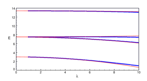
Figure 1: Eigenvalues for the first five states calculated by means of the RRM (blue points) and perturbation theory (red line)

Figure 1 shows the first five eigenvalues calculated by second-order perturbation theory and by means of the RRM. The agreement is satisfactory in a wide range of values of $\lambda$.

From the results of subsection 3.2 we conclude that

$$\lim\limits_{r_{0}\rightarrow\infty}E_{n\nu}^{(2)}=-\frac{1}{2}.$$ (22)

Table 7 shows that $E_{n\nu}^{(0)}$ tends to $2n+\nu+1$ and $E_{n\nu}^{(2)}$ to $-0.5$ as $r_{0}$ increases.

5 Conclusions

We have shown that the incomplete basis set used by Cruz et al[1] is not suitable for large values of $r_{0}$ and $\lambda$. We proposed two alternative basis sets of functions; one of them leads to simpler matrix elements but is rather inefficient for large values of the box radius. The other one leads to somewhat more complicated matrix elements but requires smaller values of $N$ in order to obtain accurate results for large values of $r_{0}$. In addition to producing quite accurate eigenvalues the RRM with these basis sets proved useful for the study of the behaviour of the spectrum of the model for very small and very large values of the box size. We also obtained reasonably accurate eigenvalues by means of second-order perturbation theory.

Table 1: Eigenvalues for the even solutions when $r_{0}=1$, $\lambda=0.05$ and $i\leq N$

$N$	$E_{1}^{(e)}$	$E_{2}^{(e)}$	$E_{3}^{(e)}$	$E_{4}^{(e)}$
$2$	$3.000033048$	$7.586264543$	$14.23335748$	$16.45868556$
$3$	$2.999983516$	$7.508025752$	$13.45385988$	$15.41429625$
$4$	$2.999940526$	$7.507311498$	$13.39694464$	$15.40025129$
$5$	$2.999940524$	$7.507179152$	$13.39164826$	$15.39159676$
$6$	$2.999940512$	$7.507178210$	$13.39154151$	$15.39154827$
$7$	$2.999940512$	$7.507178149$	$13.39153360$	$15.39153048$
$8$	$2.999940512$	$7.507178149$	$13.39153353$	$15.39153043$
$9$	$2.999940512$	$7.507178149$	$13.39153353$	$15.39153042$
$10$	$2.999940512$	$7.507178149$	$13.39153353$	$15.39153042$
Ref. [1]	$2.999940$	$7.507196$	$13.391537$

Table 2: Eigenvalues for the odd solutions when $r_{0}=1$, $\lambda=0.05$ and $i\leq N$

$N$	$E_{1}^{(o)}$	$E_{2}^{(o)}$	$E_{3}^{(o)}$	$E_{4}^{(o)}$
$3$	$7.507984721$	$13.45385988$	$22.77274842$	$25.97120953$
$4$	$7.507270472$	$13.39694464$	$20.61132495$	$24.8074732$
$5$	$7.507138138$	$13.39164826$	$20.59740341$	$24.78828653$
$6$	$7.507137196$	$13.39154151$	$20.58517127$	$24.77616193$
$7$	$7.507137135$	$13.3915336$	$20.58516517$	$24.77603555$
$8$	$7.507137134$	$13.39153353$	$20.58514439$	$24.77599977$
$9$	$7.507137134$	$13.39153353$	$20.58514439$	$24.77599951$
$10$	$7.507137134$	$13.39153353$	$20.58514438$	$24.77599947$
$11$	$7.507137134$	$13.39153353$	$20.58514438$	$24.77599947$
Ref. [1]	$7.507137$	$13.391537$

Table 3: First five eigenvalues for some values of $r_{0}$ and $\lambda$

$r_{0}=1$
$\lambda$
$0.05$	$2.999940513$	$7.507137135$	$7.507178149$	$13.39153353$	$13.39153353$
$0.50$	$2.994054784$	$7.503668344$	$7.507765819$	$13.39108541$	$13.39108591$
$1.00$	$2.976261687$	$7.493165697$	$7.509507984$	$13.38971472$	$13.38972271$
$1.50$	$2.946746472$	$7.475690676$	$7.512284352$	$13.38738763$	$13.38742819$
$2.00$	$2.905712640$	$7.451286862$	$7.515910615$	$13.38404044$	$13.38416912$
$2.50$	$2.853432944$	$7.420014281$	$7.520141153$	$13.37958431$	$13.37989994$
$3.00$	$2.790238712$	$7.381948462$	$7.524679955$	$13.37390580$	$13.37456372$
$3.50$	$2.716507923$	$7.337179290$	$7.529192808$	$13.36686757$	$13.36809331$
$4.00$	$2.632652970$	$7.285809695$	$7.533319836$	$13.35830959$	$13.36041264$
$4.50$	$2.539108909$	$7.227954221$	$7.536687533$	$13.34805070$	$13.35143815$
$5.00$	$2.436322782$	$7.163737522$	$7.538919695$	$13.33589085$	$13.34108027$
$5.50$	$2.324744395$	$7.093292825$	$7.539646842$	$13.32161397$	$13.32924491$
$6.00$	$2.204818732$	$7.016760401$	$7.538513927$	$13.30499156$	$13.31583500$
$r_{0}=2$
$0.05$	$1.121533076$	$2.471308473$	$2.471677189$	$4.092484156$	$4.092484253$
$0.50$	$1.055749927$	$2.425491724$	$2.461288707$	$4.079919270$	$4.080859951$
$1.00$	$0.8676905872$	$2.290990158$	$2.423192111$	$4.029818289$	$4.043205109$
$1.50$	$0.5825348562$	$2.079035409$	$2.345604043$	$3.921386314$	$3.974310688$
$2.00$	$0.2240418306$	$1.802394297$	$2.221750826$	$3.750830242$	$3.869531452$
$2.50$	$-0.1898793720$	$1.472757021$	$2.051207036$	$3.528077680$	$3.726784048$
$3.00$	$-0.6466661902$	$1.099674893$	$1.836953799$	$3.263614113$	$3.546435112$
$3.50$	$-1.137519525$	$0.6906132774$	$1.583000466$	$2.965401619$	$3.330401976$
$4.00$	$-1.656139155$	$0.2513481407$	$1.293278752$	$2.639409865$	$3.081315858$
$4.50$	$-2.197888537$	$-0.2136268090$	$0.9712902180$	$2.290243036$	$2.801986817$
$5.00$	$-2.759263211$	$-0.7007731576$	$0.6200711870$	$1.921520387$	$2.495126178$
$5.50$	$-3.337549806$	$-1.207265044$	$0.2422612717$	$1.536106044$	$2.163228074$
$6.00$	$-3.930602471$	$-1.730813281$	$-0.1598114054$	$1.136262144$	$1.808534720$
$r_{0}=3$
$0.05$	$1.000719415$	$2.013820524$	$2.013958910$	$3.057224946$	$3.057227051$
$0.50$	$0.8810998253$	$1.901568472$	$1.916966478$	$2.965602260$	$2.977378029$
$1.00$	$0.5302449413$	$1.575816276$	$1.649888731$	$2.680883025$	$2.751206873$
$1.50$	$-0.01534172516$	$1.074370141$	$1.261029544$	$2.240275829$	$2.407990915$
$2.00$	$-0.7078968358$	$0.4396646394$	$0.7809055363$	$1.681527101$	$1.968686336$
$2.50$	$-1.505217743$	$-0.2930063285$	$0.2246424266$	$1.035590763$	$1.446909507$
$3.00$	$-2.377395710$	$-1.098385329$	$-0.3990488847$	$0.3264125547$	$0.8529729025$
$3.50$	$-3.304713209$	$-1.959183144$	$-1.084579031$	$-0.4273630821$	$0.1956863049$
$4.00$	$-4.274142731$	$-2.863493879$	$-1.828291585$	$-1.211048117$	$-0.5170228781$
$4.50$	$-5.276820708$	$-3.802913311$	$-2.626732853$	$-2.014028483$	$-1.277913746$
$5.00$	$-6.306499209$	$-4.771332759$	$-3.474706132$	$-2.830565891$	$-2.080445685$
$5.50$	$-7.358622358$	$-5.764184603$	$-4.365053586$	$-3.659193962$	$-2.918861635$
$6.00$	$-8.429766567$	$-6.777965138$	$-5.290258763$	$-4.500526982$	$-3.788232221$

Table 4: $r_{0}^{2}E$ for $r_{0}=0.01$

$r_{0}^{2}E$	$E^{PB}$
$2.891592982$	$2.891592981$
$7.340985322$	$7.340985321$
$13.18730821$	$13.18730821$
$15.23563117$	$15.23563117$

Table 5: Eigenvalue $E_{00}$ for increasing values of $r_{0}$ and some values of $\lambda$

$r_{0}$	$\lambda=1$	$\lambda=2$	$\lambda=3$	$\lambda=4$	$\lambda=5$
$1$	$2.9762616872$	$2.9057126397$	$2.7902387123$	$2.6326529698$	$2.4363227822$
$2$	$0.8676905872$	$0.2240418306$	$-0.6466661902$	$-1.6561391549$	$-2.7592632114$
$3$	$0.5302449413$	$-0.7078968358$	$-2.3773957102$	$-4.2741427314$	$-6.3064992087$
$4$	$0.5003869888$	$-0.9754437781$	$-3.2281562207$	$-5.9149227688$	$-8.8273550313$
$5$	$0.5000005484$	$-0.9996955349$	$-3.4775005103$	$-6.7378369178$	$-10.4347543324$
$6$	$0.5000000001$	$-0.9999995776$	$-3.4997274446$	$-6.97857932$	$-11.24353629$
$\infty$	$0.5$	$-1$	$-3.5$	$-7$	$-11.5\par$

Table 6: First two coefficients of the perturbation expansion for the lowest energies when $r_{0}=1$

$E^{(0)}$	$E^{(2)}$
$3.00000000000000000000000000000$	$-0.0237951331606905590236056369694$
$7.50717218045194296125597056932$	$-0.0140183043464296058590713039161$
$7.50717218045194296125597056932$	$0.00238755957790725763825593365598$
$13.3915380494648018553204940093$	$-0.00180627777546582495721462311771$
$13.3915380494648018553204940093$	$-0.00180627777546582495721462311771$

Table 7: $E_{n,\nu}^{(0)}$ and $E_{n,\nu}^{(2)}$ for increasing values of $r_{0}$

$r_{0}$	$E_{00}^{(e,0)}$	$E_{10}^{(e,0)}$	$E_{20}^{(e,0)}$	$E_{01}^{(e,0)}$	$E_{11}^{(e,0)}$	$E_{02}^{(e,0)}$
1	3.00000000	15.39153805	37.60583487	7.50717218	24.77601000	13.39153805
2	1.12220853	4.44050521	10.01698219	2.47177521	6.82577445	4.09259935
3	1.00193679	3.08886540	5.68860128	2.01496711	4.27163834	3.05805047
4	1.00000336	3.00063504	5.02056599	2.00004978	4.00395689	3.00036610
5	1.00000000	3.00000035	5.00003719	2.00000002	4.00000378	3.00000019

$r_{0}$	$E_{01}^{(o,0)}$	$E_{11}^{(o,0)}$	$E_{02}^{(o,0)}$
1	7.50717218	24.77601000	13.39153805
2	2.47177521	6.82577445	4.09259935
3	2.01496711	4.27163834	3.05805047
4	2.00004978	4.00395689	3.00036610
5	2.00000002	4.00000378	3.00000019

$r_{0}$	$E_{00}^{(e,2)}$	$E_{10}^{(e,2)}$	$E_{20}^{(e,2)}$	$E_{01}^{(e,2)}$	$E_{11}^{(e,2)}$	$E_{02}^{(e,2)}$
1	-0.02379513	-0.00304969	-0.00116231	0.00238756	0.00085352	-0.00180628
2	-0.27022732	-0.04303208	-0.01639429	-0.03917956	0.01445894	-0.04603071
3	-0.48698448	-0.27520028	-0.06592876	-0.40340299	-0.03096954	-0.32944152
4	-0.49995340	-0.49391191	-0.39406165	-0.49914014	-0.45745249	-0.49638216
5	-0.49999998	-0.49999345	-0.49945600	-0.49999951	-0.49990653	-0.49999640

$r_{0}$	$E_{01}^{(o,2)}$	$E_{11}^{(o,2)}$	$E_{02}^{(o,2)}$
1	-0.01401830	-0.00420907	-0.00180628
2	-0.18671149	-0.06215340	-0.04603071
3	-0.45868737	-0.25480400	-0.32944152
4	-0.49968212	-0.48373136	-0.49638216
5	-0.49999983	-0.49996665	-0.49999640

References

• [1] E. Cruz, N. Aquino, V. Prasad, and A. Flores-Riveros, Eur. Phys. J. D 78, 71 (2024).
• [2] F. L. Pilar, Elementary Quantum Chemistry (McGraw-Hill, New York, 1968).
• [3] A. Szabo and N. S. Ostlund, Modern Quantum Chemistry (Dover Publications, Inc., Mineola, New York, 1996).
• [4] J. K. L. MacDonald, Phys Rev. 43, 830 (1933).
• [5] F. M. Fernández, On the Rayleigh-Ritz variational method, arXiv:2206.05122 [quant-ph].
• [6] F. M. Fernández, Dimensionless equations in non-relativistic quantum mechanics, arXiv:2005.05377 [quant-ph].
• [7] H. E. Montgomery Jr., G. Campoy, and N. Aquino, Phys. Scr. 81, 045010 (2010).
• [8] F. M. Fernández, J. Math. Chem. (2024). doi.org /10.1007/s10910-024-01644-2, doi:10.20944/preprints202405.1006.v1.
• [9] F. M. Fernández and J. Garcia, Cent. Eur. J. Phys. 12, 554 (2014).
• [10] F. M. Fernández, Introduction to Perturbation Theory in Quantum Mechanics (CRC Press, Boca Raton, 2001).