Abstract

The basic equations, concepts, and modes of linear, ideal, MHD waves – slow, Alfvén and fast – are set out and generalised to gravitationally-stratified atmospheres. Particular attention is devoted to mode conversion, wherein the local behavior of a global wave changes from one mode to another in passing through particular atmospheric layers. Exact solutions are explored where available. Eikonal methods – WKBJ and ray theory – are described. Although our emphasis is on the theoretical underpinning of the subject, the solar atmospheric heating implications of fast/slow and fast/Alfvén conversions are discussed in detail.

citnum

[1]

Chapter 0 MHD Waves in Homogeneous and Continuously Stratified Atmospheres

1 Introduction

This chapter discusses the nature of waves in magnetized astrophysical fluids. Owing to its proximity and visibility, we are primarily concerned with the optically-thin solar atmosphere. However, our results and findings are widely applicable to astrophysical settings where the plasma admits a continuum or fluid-dynamical description.

The subject of magnetohydrodynamic (MHD) waves is not without its intrinsic subtleties. They result from the linearization of the fully nonlinear magnetofluid dynamics about an appropriate equilibrium state. In this sense, they obtain formally in the limit of infinitesimal amplitudes, i.e., when quadratic terms may be neglected compared to the leading-order linear terms. On the other hand, every observation is predicated upon the presence of a finite-amplitude disturbance in an astrophysical fluid. In this fashion, MHD waves are mathematical idealizations, which hopefully capture the essential behavior of small-amplitude fluctuations in actual magnetized astrophysical plasmas. The fundamental issue is which fluctuations are of sufficiently small amplitude, and which are not. Stated differently: under what conditions may the second-order quadratic terms be safely discarded?

This question must be addressed on a case-by-case basis. In turn it poses a deeper and more perplexing question: what aspects or components of a given dynamical MHD flow are to be identified with MHD waves? And to what then do we ascribe the remainder of the time-dependent flow? This is a topic of active investigation and we shall be content to simply offer a few useful insights in what follows.

The applicability of the MHD fluid description of waves is bounded in both temporal frequency and spatial wavelength, or wavenumber. At high frequencies and small wavelengths the particulate nature of the plasma must be taken into account. The plasma frequency and gyro-frequencies of the electrons and ions serve to mark this boundary between particle and collective fluid behaviors. Even collisionless plasmas may be treated as a fluid, provided care is taken in developing an accurate equation of state. Dissipative transport processes may be accommodated within the fluid picture when frequencies and wavelengths are comparable to collective relaxation times and lengths (Appendix LABEL:app:thermo). At the other extreme of low frequencies and large wavelengths, one must take care in identifying the appropriate equilibrium state. In some instances it is necessary to allow this equilibrium to evolve slowly in time or to be treated as a random medium. Such extensions of the fluid MHD wave description are beyond the scope of this chapter.

MHD waves may be modified and duly influenced by physical processes like rotation, buoyancy, and steady fluid motions, for example. The resulting menagerie of hybrid waves has spawned a vast and sometimes bewildering nomenclature. In a stellar atmosphere, the radiation field frequently exerts the dominant influence on MHD waves. It not only provides a dissipation mechanism, but in hot stars it may also modify the propagation characteristics of the waves (Appendix LABEL:app:RMHD).

1 Magneto-acoustic-gravity (MAG) Waves in the Combined Photosphere/Chromosphere

A rich variety of oscillations and waves are observed between the base of the solar corona and the surface of the Sun (00bogdan; Rut03aa; 06bogdan; 15khomenko; 16lohner; 21srivastava; JesJafKey23aa). The solar convection and its overshoot are the primary mechanical sources that generate these disturbances. Intermittent flares of all scales throughout, and above, this roughly 2 Mm-thick optically-thin atmospheric layer are also wave sources. Generally speaking, these waves are able to partially pass through the upper and lower boundaries of the combined photosphere and chromosphere. In both directions they encounter a rapid increase in the average plasma temperature and characteristic vertical (radial) density scale-height.

Indeed, what sets the combined photosphere/chromosphere apart from the neighboring corona and convection zone is its low temperatures ($T\approx 4000-6000$ K) and small scale-heights ($H_{\rho}\approx 150-200$ km). These attributes pose serious challenges to modeling magneto-acoustic-gravity (MAG) waves. Structures like granules, pores, sunspots and the magnetic network exhibit horizontal scales that are very much larger than $H_{\rho}$. This effectively breaks the translational symmetry that might otherwise permit Fourier analysis in the vertical (i.e., radial) direction. As we shall presently demonstrate, this in turn necessitates the solution of ordinary differential equations (ODEs) with non-constant coefficients.

A second complication is provided by the convective overshoot. The photosphere/chromosphere may be regarded as a solar ‘surf-zone’ where the inertia of episodic convective upflows carries them far into the overlying stable atmosphere before buoyancy breaking eventually halts their progress (95carlsson; 11uitenbroek; 13criscuoli). Spicules and umbral flashes are familiar observational signatures of these processes. Mass balance ensures a gradual subsidence of the dense material back to the convection zone. Therefore, the photosphere/chromosphere is dynamic in a chaotic sense. Flares and coronal transients are additional sources of chaotic dynamics. The photospheres and chromospheres of stars with convective envelopes must sustain similar conditions. Finally, as Lighthill, Proudman, Parker and Kulsrud have all pointed out, this chaotic dynamics will in turn generate waves and oscillations in situ (52lighthill; 52proudman; 53parker; 54lightill; 55kulsrud). See GolMurKum94aa and references therein for more recent developments.

Coherent waves and oscillations with sufficiently large wavelengths and long periods will emerge from and propagate through these optically-thin stellar surf-zones. For the Sun, the dominant temporal periods are on the order of a few minutes. Horizontal wavelengths cover a much broader range from fractions of a solar radius down to a few tenths of a second of arc (comparable to the density scale-height in the photosphere). As Dewar noted, large-scale coherent waves/oscillations sample the physical conditions in the chaotic photosphere/chromosphere surf-zone in a fashion that depends upon their individual nature and they adjust their properties accordingly (70dewar; 71dewar). The ‘wave mean’ of a physical quantity, like the (vector) magnetic field, the adiabatic compressibility, or advective flow, for example, may be distinct from simple (i.e., unweighted) spatial and temporal averages. This adds further subtlety to the analysis and complicates spectropolarimetric inversions.

We shall simply refer to periodic fluctuations detected in the solar photosphere/chromosphere as MAG waves or oscillations because the principal restoring forces are some combination of magnetic pressure/tension, plasma compressibility, and gravitational stratification/buoyancy. Except in special circumstances, radiative transfer, fluid viscosity, thermal conduction, ohmic dissipation, and solar rotation will have a lesser, or secondary, influence.

The first detection of solar MAG waves came in the late 1960s (69beckers; 74schultz). Since then, they have received a rapidly expanding amount of attention and careful study. This has been facilitated by advances in instrumentation – larger telescope apertures, faster CCDs, precision spectropolarimetry, broad spectral access from space – and computational advances. Indeed, entire disciplines, such as astero- and helioseismology emerged and have now become mature areas of study. Offshoots, like the seismology of spots and coronae are flourishing.

For several reasons, attention has focused on waves and oscillations with periods between 1 and 10 minutes. These waves exhibit characteristic ridge or ring structures in traditional $k$–$\omega$ power-spectra diagrams. At both larger and smaller oscillation periods these coherent structures fade into an incoherent continuum of oscillations with random phases, amplitudes, and wavevectors. Apropos the question raised in the introduction, these power spectra contain large contributions from the turbulent convection in addition to waves.

We can do no better than simply point the reader to several current reviews on these topics (02jcdc; 16basu; 21brown). However, a few cautionary remarks will be helpful for what follows. First, there are clear differences between the periodic fluctuations detected in strong (and perhaps laminar, unipolar) magnetic fields (i.e., the umbrae of spots), and the surrounding quiet Sun. No doubt, there are ample ‘salt-and-pepper’ magnetic fields present throughout the quiet Sun. In contrast to the umbral magnetic fields, they are turbulent, bipolar, randomly-oriented, and possibly fibril (or better, intermittent) in nature. Inclined penumbrae lie somewhere between these two extremes. This observational dichotomy suggests, à la Dewar, that the waves/oscillations take rather different averages of these two extreme states of solar surface magnetism. Second, it is necessary to distinguish between the bona fide propagation of a disturbance and the sequential emergence of a disturbance’s wave-front through a particular atmospheric surface where a spectral diagnostic is formed. A good case in point is the phenomenon of running penumbral waves. Third, the theory of MAG waves invokes the mathematical limit of letting the wave amplitude tend to zero, whilst any observed fluctuation must necessarily have a finite amplitude. Chromospheric umbral flashes, for example, are most certainly nonlinear wave-trains that have steepened into shocks.

2 Overview

In this chapter we first introduce the basic equations of MHD waves and then derive their simple iconic forms (slow, Alfvén and fast) in a uniform, translationally-invariant, plasma. These iconic forms have the distinct pedagogical advantage that the governing partial differential equations (PDEs) factor into three distinct decoupled forms, or wave-modes.

We then focus primarily on what is perhaps the dominant departure from this simple picture pertaining to the low solar atmosphere: gravitational stratification in the vertical direction, giving rise to magneto-acoustic-gravity (MAG) waves which may only locally adhere to the fast-Alfvén-slow trichotomy. Indeed, the essential point is that the governing PDEs do not in general factor, or decouple, unless the equilibrium possesses one or more translational symmetries.

Instead, one may be able to identify spatial domains where one of the wave-modes is only weakly-coupled to the remainder. Globally, these MAG waves exhibit mixed characteristics at different locations. This may be conveniently regarded as the result of wave mode-conversion processes. We shall presently enumerate and illustrate the various mode-conversion processes.

In general, however, when no spatial symmetries are present in the equilibrium, the governing wave PDEs do not decouple and the characterization and classification of the resulting MAG waves is distinctly equilibrium-dependent. Such problems are of course the most germane to astrophysical situations. They are invariably treated by numerical methods.

Other chapters in this volume address important deviations from this elementary scenario, such as flux tubes (Chapter 5), partial ionization (Chapter 6) and nonlinearities (Chapter 8). All of these aspects contribute to the important topics of coronal heating (Chapter 10) and solar wind acceleration (Chapter 11).

2 MHD Equations

The single-fluid MHD equations are commonly expressed in terms of the density $\rho$, plasma velocity ${\mathbf{v}}$, magnetic induction ${\mathbf{B}}$, current density $\mathbf{j}=\mu^{-1}\mbox{\boldmath$\nabla$}{\boldsymbol{\times}}\hskip 1.5pt{\mathbf{B}}$ (current per unit area), and gravitational acceleration $\mathbf{g}$. In solar physics, ${\mathbf{B}}$ is normally called the magnetic field, though strictly, in a macroscopic medium, the magnetic field $\mathbf{H}$ is related to the magnetic induction ${\mathbf{B}}$ via a constitutive relation ${\mathbf{B}}=\mu\mathbf{H}$, but in astrophysical plasmas $\mu$ is accurately represented by its vacuum value $\mu_{0}=4\pi\times 10^{-7}$ $\rm H\,m^{-1}$ in SI units, and $\mathbf{H}$ plays no independent role.

1 Conventional Form

Mass conservation is expressed by

$$\frac{\mathrm{D}\rho}{\mathrm{D}t}+\rho\mbox{\boldmath$\nabla$}{\boldsymbol{\cdot}}\hskip 1.5pt{\bf v}=0,$$ (1)

familiar from hydrodynamics, where

$$\frac{\mathrm{D}\phantom{t}}{\mathrm{D}t}=\frac{\partial\phantom{t}}{\partial t}+{\bf v}\hskip 1.5pt{\boldsymbol{\cdot}}\mbox{\boldmath$\nabla$}$$ (2)

is the comoving derivative.

Similarly, the momentum equation also carries over from neutral fluid theory,

$$\rho\frac{\mathrm{D}{\mathbf{v}}}{\mathrm{D}t}=-\mbox{\boldmath$\nabla$}p+{\mathbf{j}\,{\boldsymbol{\times}}\,{\mathbf{B}}}+\rho\,\mathbf{g}+\eta_{v}\nabla^{2}{\bf v}+\left(\zeta+\frac{1}{3}\eta_{v}\right)\mbox{\boldmath$\nabla$}\left(\mbox{\boldmath$\nabla$}{\boldsymbol{\cdot}}\hskip 1.5pt{\bf v}\right),$$ (3)

though with the addition of the Lorentz force ${\mathbf{j}\,{\boldsymbol{\times}}\,{\mathbf{B}}}$, which may be decomposed into magnetic pressure gradient and magnetic tension components $-\mbox{\boldmath$\nabla$}(B^{2}/2\mu)+\mbox{\boldmath$\nabla$}{\boldsymbol{\cdot}}\hskip 1.5pt({\mathbf{B}}{\mathbf{B}}/\mu)$. The gravitational acceleration $\mathbf{g}=-\mbox{\boldmath$\nabla$}\phi$ is normally specified externally, but can be calculated self-consistently using the Poisson equation $\nabla^{2}\phi=4\pi G\rho$ for a self-gravitating system. For completeness, the coefficients of dynamic and bulk viscosity $\eta_{v}$ and $\zeta$ have been included, though these are negligible in most solar contexts and will be dropped hereafter. The momentum equation describes how the magnetic field affects the plasma’s motion.

Conversely, the flow of plasma also affects the magnetic field, as described by the induction equation

$$\frac{\partial{\mathbf{B}}}{\partial t}=\mbox{\boldmath$\nabla$}{\boldsymbol{\times}}\left({\mathbf{v}}\,{\boldsymbol{\times}}\,{\mathbf{B}}\right)-\mbox{\boldmath$\nabla$}{\boldsymbol{\times}}\!\left(\eta\mbox{\boldmath$\nabla$}{\boldsymbol{\times}}\hskip 1.5pt{\mathbf{B}}\right),$$ (4)

where $\eta=1/\mu\sigma$ is the magnetic diffusivity and $\sigma$ is the electrical conductivity. If $\eta$ is uniform, this is more commonly expressed in the form

$$\frac{\partial{\mathbf{B}}}{\partial t}=\mbox{\boldmath$\nabla$}{\boldsymbol{\times}}\!\left({\mathbf{v}}\,{\boldsymbol{\times}}\,{\mathbf{B}}\right)+\eta\nabla^{2}{{\mathbf{B}}},$$ (5)

from which the diffusive nature of $\eta$ is apparent. We shall also neglect the magnetic diffusivity, restricting attention to so-called ideal MHD.

2 Conservation Form

For numerical purposes, and also when deriving the jump conditions for shock waves (see Chapter 9), the MHD equations are more useful in conservation form $\partial\mbox{`density'}/\partial t+\mbox{div`flux'}=0$, where ‘density’ is some scalar or vector quantity per unit volume and ‘flux’ is a vector or dyadic generalized flux of the same quantity.

For example, the mass conservation equation for density $\rho$ takes the form

$$\frac{\partial\rho}{\partial t}+\mbox{\boldmath$\nabla$}{\boldsymbol{\cdot}}\hskip 1.5pt(\rho{\mathbf{v}})=0,$$ (6)

with $\rho{\mathbf{v}}$ being the mass flux per unit volume. Similarly, momentum conservation may be expressed as

$$\frac{\partial\rho{\mathbf{v}}}{\partial t}+\mbox{\boldmath$\nabla$}{\boldsymbol{\cdot}}\hskip 1.5pt\mathbf{T}=-\rho\mbox{\boldmath$\nabla$}\phi,$$ (7)

where $\phi$ is the gravitational potential such that $\mathbf{g}=-\mbox{\boldmath$\nabla$}\phi$, and the non-zero right hand side indicates that momentum is in fact not conserved in an external gravitational field. The dyadic

$$\mathbf{T}=\rho{\mathbf{v}}{\mathbf{v}}+\left(p+\frac{B^{2}}{2\mu}\right){\mathbf{I}}-\frac{{\mathbf{B}}{\mathbf{B}}}{\mu}$$ (8)

is the total stress tensor, where ${\mathbf{I}}$ is the $3\times 3$ identity. The ideal induction equation may also be written in conservation form,

$$\frac{\partial{\mathbf{B}}}{\partial t}+\mbox{\boldmath$\nabla$}{\boldsymbol{\cdot}}\left({\mathbf{v}}{\mathbf{B}}-{\mathbf{B}}{\mathbf{v}}\right)=0,$$ (9)

since magnetic flux is conserved. Finally, the total energy equation expresses the Eulerian time derivative of the local energy density $U={\textstyle\frac{1}{2}}\rho v^{2}+p/(\gamma-1)+B^{2}/2\mu+\rho\phi$ (kinetic+thermal+magnetic+gravitational) in terms of the divergence of the total energy flux $\mathbf{f}$

$$\frac{\partial U}{\partial t}+\mbox{\boldmath$\nabla$}{\boldsymbol{\cdot}}\hskip 1.5pt\mathbf{f}=0$$ (10)

where

$$\mathbf{f}=\left({\textstyle\frac{1}{2}}\rho\hskip 1.5ptv^{2}+\frac{\gamma}{\gamma-1}p+\rho\phi\right)\!{\mathbf{v}}-\frac{1}{\mu}({\mathbf{v}}{\boldsymbol{\times}}{\mathbf{B}}){\boldsymbol{\times}}{\mathbf{B}}~{},$$ (11)

and $\gamma$ is the ratio of specific heats. This flux corresponds to the sum of the advected kinetic, thermal and gravitational energies, the rate of working of the pressure force $p{\mathbf{v}}$, and the electromagnetic (Poynting) flux, $\mu^{-1}{\mathbf{E}}{\boldsymbol{\times}}{\mathbf{B}}$, where ${\mathbf{E}}=-{\mathbf{v}}{\boldsymbol{\times}}{\mathbf{B}}$ (in ideal MHD) is the electric field.

Often the first law of thermodynamics is invoked to provide an alternate but equivalent form of these last two equations couched in terms of conservation of specific entropy $\eta$ of the fluid,

$$\rho\,T\,\frac{\mathrm{D}\eta}{\mathrm{D}t}=-\mathcal{L},$$ (12)

where $\mathcal{L}$ is the net energy loss per unit volume (outgoing minus incoming), made up of radiation, conduction, viscous, Joule, etc. terms (Appendices LABEL:app:thermo, LABEL:app:RMHD). In the absence of heating or loss, specific entropy and energy are conserved following the motion.

3 MHD Equilibria

1 Lorentz Force and Equilibrium

Setting ${\mathbf{v}}=\mathbf{0}$ in the momentum equation (3) results in the equation of magnetohydrostatic (MHS) equilibrium,

$$\mathbf{0}=-\mbox{\boldmath$\nabla$}p+{\mathbf{j}\,{\boldsymbol{\times}}\,{\mathbf{B}}}+\rho\,\mathbf{g}.$$ (13)

In all but some very simple symmetric scenarios this equation is challenging to solve. The essential difficulty is the Lorentz force must be the gradient of a scalar (pressure) in every two-dimensional manifold perpendicular to g. This is difficult to arrange in principle (85low; 86bogdan; 99neukirch; 05low), and as Parker has demonstrated, essentially impossible to achieve in practice (94parker).

To appreciate this equation, one must understand the Lorentz force (actually a force per unit volume), ${\mathbf{F}}_{\text}{L}=\mathbf{j}\,{\boldsymbol{\times}}\,{\mathbf{B}}=\mu^{-1}(\mbox{\boldmath$\nabla$}{\boldsymbol{\times}}\hskip 1.5pt{\mathbf{B}}){\boldsymbol{\times}}\,{\mathbf{B}}$. Taking a curl and then a cross product of a known magnetic field in one’s head, especially if expressed in cartoon form, is probably beyond most of us, so how can we understand the Lorentz force for a given sketched ${\mathbf{B}}$?

Using standard vector identities, we may recast

$${\mathbf{F}}_{\text}{L}={\mathbf{B}}\,{\boldsymbol{\cdot}}\mbox{\boldmath$\nabla$}\,{\mathbf{B}}/\mu-\mbox{\boldmath$\nabla$}(B^{2}/2\mu),$$ (14)

which can be interpreted respectively as a magnetic tension force along field lines, and a magnetic pressure force $-\mbox{\boldmath$\nabla$}p_{\text}{mag}$ where $p_{\text}{mag}=B^{2}/2\mu$ is the magnetic pressure. Hence Equation (13) can be rewritten as

$$\mathbf{0}=-\mbox{\boldmath$\nabla$}\left(p+p_{\text}{mag}\right)+{\mathbf{B}}\,{\boldsymbol{\cdot}}\mbox{\boldmath$\nabla$}\,{\mathbf{B}}/\mu+\rho\,\mathbf{g},$$ (15)

making the equilibrium balance between total pressure $p+p_{\text}{mag}$, tension and gravity more intuitive. We mention in passing that $B^{2}/2\mu$ is also the magnetic energy density, and the Lorentz force can also be expressed as the divergence of the symmetric Maxwell stress tensor.

In the solar corona, magnetic energy density typically exceeds thermal energy density by an order of magnitude, so it a reasonable approximation to set ${\mathbf{F}}_{\text}{L}=\mathbf{0}$ to obtain a (near) equilibrium. Any ${\mathbf{B}}$ satisfying this condition is called a force free field, of which there are several types.

The simplest are potential fields, ${\mathbf{B}}=\mbox{\boldmath$\nabla$}\Phi$ for some harmonic scalar potential $\Phi$, i.e., where $\nabla^{2}\Phi=0$. Then $\mathbf{j}=\mu^{-1}\mbox{\boldmath$\nabla$}{\boldsymbol{\times}}\hskip 1.5pt{\mathbf{B}}=\mathbf{0}$, by the standard vector field result that the curl of a gradient always vanishes. This trivially makes the Lorentz force zero. It can be shown that a potential field in a closed volume with $B_{n}=\hat{\mathbf{n}}\,{\boldsymbol{\cdot}}\,{\mathbf{B}}$ specified on its boundary (unit normal $\hat{\mathbf{n}}$) is unique and has the minimum possible energy, making it globally stable. This is also true external to a closed surface such as the entire solar photosphere over which $B_{n}$ is prescribed if $B\to 0$ as radius $r\to\infty$ is also assumed. Another name for a potential field is a current free field.

The other way that a magnetic field can be force free is if the current is parallel to ${\mathbf{B}}$, since the cross product of parallel vectors always vanishes. Thus we may write $\mbox{\boldmath$\nabla$}{\boldsymbol{\times}}{\mathbf{B}}=\alpha\,{\mathbf{B}}$ for some scalar function of position $\alpha$. However, $\alpha$ cannot be arbitrary. Recall that $\mbox{\boldmath$\nabla$}{\boldsymbol{\cdot}}\hskip 1.5pt{\mathbf{B}}=0$ and div curl is always zero, so ${\mathbf{B}}\,{\boldsymbol{\cdot}}\,\mbox{\boldmath$\nabla$}\alpha=0$. But this is a directional derivative meaning that $\alpha$ must be constant along field lines. The particular case where all field lines have the same $\alpha$ is called a constant-$\alpha$ field, for which (by a standard vector identity) $(\nabla^{2}+\alpha^{2}){\mathbf{B}}=0$: the vector Helmholtz equation.

A simple example of a non-force-free MHS equilibrium, with gas pressure $p$ but no gravity, is the case of a non-uniform magnetic slab ${\mathbf{B}}=(0,0,B(x))$ for which total pressure $p(x)+B^{2}(x)/2\mu$ is uniform, since there are no net tension or pressure forces.

These insights can be invaluable when constructing force-free or MHS model equilibria for exploring waves. Of course, the Sun is a very dynamic place, and is certainly not in equilibrium. Nevertheless, there are large-scale magnetic structures (sunspot fields, coronal holes, systems of coronal loops, etc.) that persist for much longer than the wave-crossing times on which they might be expected to evolve. In this sense, a time-independent, static, magneto-atmosphere is a reasonable first approximation to what is at best a statistically steady equilibrium.

2 Energy, Variational Principles and Stability

Of course, a MHS equilibrium – where all forces balance – may not be stable. A marble sitting on top of a smooth hill, or even a smooth saddle, may well be in equilibrium, but it is not stable, since there are tiny perturbations that could be made to its position or velocity that would see it run away down the hill.

This may hold for MHS equilibria too. If an equilibrium is such that all allowable infinitesimal perturbations to its state subsequently move back towards the equilibrium, the system is said to be linearly stable. This is a necessary but not sufficient condition for global stability, i.e., stability to all perturbations, no matter how large.

To determine if a particular equilibrium is linearly stable, we must make a general linear perturbation to its state, for example by imposing a small non-zero velocity ${\mathbf{v}}$. This results in the Ferraro-Plumpton equation (2) for MAG waves to be derived in Section 2 from the MHD differential equations. The details do not concern us here, but the upshot is an equation of the form

$$\frac{\partial^{2}{\mathbf{v}}}{\partial t^{2}}=-{\mathbf{G}}[{\mathbf{v}}]$$ (16)

for a particular self-adjoint linear force operator ${\mathbf{G}}$ (GoePoe04aa, Section 6.2.3).

This linear perturbation equation may be Fourier transformed from the time $t$ to the frequency $\omega$ domain. In other words, we build ${{\mathbf{v}}}({\mathbf{x}},t)$ from a weighted superposition of Fourier modes

$${\mathbf{V}}(\mathbf{x},\omega)\exp\left[-i\omega t\right],$$ (17)

where it is convenient to introduce the Lagrangian displacement of a parcel of fluid from its equilibrium position defined by

$$\mbox{\boldmath$\xi$}(\mathbf{x},\omega)\equiv\frac{i}{\omega}{\mathbf{V}}(\mathbf{x},\omega)~{}.$$ (18)

The Fourier-transformed Ferraro-Plumpton equation then takes the compact form

$$\omega^{2}\mbox{\boldmath$\xi$}={\mathbf{G}}[\mbox{\boldmath$\xi$}]~{}.$$ (19)

The Energy Principle of FriRot60aa follows by taking the usual (Euclidean) dot-product of both sides of this equation with $\rho\mbox{\boldmath$\xi$}^{*}$, and integrating over $\mathbf{x}$. This yields the familiar Rayleigh-Ritz formula for the square of the frequency:

$$\omega^{2}=\frac{\langle\mbox{\boldmath$\xi$}^{*},{\mathbf{G}}[\mbox{\boldmath$\xi$}]\rangle}{\langle\mbox{\boldmath$\xi$}^{*},\mbox{\boldmath$\xi$}\rangle}~{},$$ (20)

provided any surface-integrals may be neglected. If any Lagrangian displacement can be found for which the right-side of this equation is negative, then the equilibrium (encoded in the self-adjoint operator ${\mathbf{G}}$) is unstable. Otherwise, this expression can be used to estimate the oscillation frequencies of an isolated magnetostatic equilibrium, because the right-side of this equation is second-order in the difference between the actual (usually unknown) Lagrangian displacement $\xi$, and any surrogate.

Finally, we note that the actual Lagrangian displacement is an extremum of the action,

$$S[\mbox{\boldmath$\xi$}]=\int\!d\mathbf{x}\,dt~{}\rho(\mathbf{x})\left(\frac{\partial\mbox{\boldmath$\xi$}}{\partial t}\,{\boldsymbol{\cdot}}\,\frac{\partial\mbox{\boldmath$\xi$}}{\partial t}-\mbox{\boldmath$\xi$}\,{\boldsymbol{\cdot}}\,{\mathbf{G}}[\mbox{\boldmath$\xi$}]\right)~{},$$ (21)

where here $\xi$ has not been Fourier transformed and so is real; see, for example 16ogilvie; 16keppens1; 16keppens2. The Ferraro-Plumpton equation may be found variationally by setting $\delta S=0$ (FerPlu58aa; Tho83aa).

4 What are MHD Waves?

1 Basic Equations

Waves result from the interplay of fluid inertia and restoring forces. In this chapter, we restrict attention to linear waves. Variables such as the density $\rho$ are written as $\rho_{0}+\rho_{1}+\rho_{2}+\cdots$. The subscript ‘0’ indicates the equilibrium value and the subscript ‘1’ denotes a small perturbation, $\rho_{1}\ll\rho_{0}$. Terms of quadratic or higher order in the perturbation quantities are ‘neglected’ in the sense that they usually serve as source terms which may be prescribed ab initio. If the equilibrium is stationary, then ${\mathbf{v}}={\mathbf{v}}_{1}$ is intrinsically small, so $\rho_{1}{\mathbf{v}}$ for example is dropped, or perhaps accommodated in a source term.

The existence of magnetohydrodynamic waves was first predicted from theory over 80 years ago (Alf42aa; Rus18mk). They assume their simplest form in a homogeneous ideal-gas fluid permeated by a uniform magnetic field. If this medium is perturbed from its stable equilibrium, the linearized MHD equations take the form ∂ρ1∂t+ρ_0$\nabla$⋅ v=0,
ρ_0∂v∂t=-$\nabla$p_1+1μ($\nabla$× B_1)× B_0,
∂p1∂t-c^2∂ρ1∂t = (γ-1)ρ_0 T_0 ∂η1∂t = 0,
∂B1∂t=$\nabla$×​(v × B_0),
$\nabla$⋅ B_1=0, where $c=\sqrt{\gamma p_{0}/\rho_{0}}$ is the adiabatic sound speed, $T$ is the temperature (units: Kelvins), and $\eta$ is the specific entropy (units: Joules kg^-1 Kelvin^-1). We do not explicitly write out the source terms in the conservation equations for mass, momentum, and entropy as they may assume different forms based on a given application. Without such terms or inhomogeneous initial or boundary conditions, these equation have only the trivial solution.

A very useful property of these equations is the existence of a wave-energy/flux conservation law which is quadratic in the wave amplitudes:

$$\frac{\partial U_{2}}{\partial t}+\mbox{\boldmath$\nabla$}{\boldsymbol{\cdot}}\hskip 1.5pt{{\bf f}_{2}}=0,$$ (22)

where U_2 = 12 ρ_0 v^2 + p122ρ0c2 + 12μ B_1^2 ,
f_2 = p_1 v + 1μ ( B_0 ⋅B_1 ) v - 1μ( v ⋅B_1) B_0 . The wave energy-flux, ${\bf f}_{2}$, permits one to assess the potential for MHD waves to heat a stellar atmosphere. Notice that the wave energy-density is distributed across kinetic, thermal and magnetic reservoirs. The wave-energy/flux conservation law also applies to pure acoustic waves (${\mathbf{B}}_{0}=\mathbf{0}$).

Differentiating Equation (1) with respect to time and eliminating $\rho_{1}$, $p_{1}$, and ${\mathbf{B}}_{1}$ in favour of $\bf v$ using the remaining equations, we find

$$\frac{\partial^{2}{\mathbf{v}}}{\partial t^{2}}=c^{2}\mbox{\boldmath$\nabla$}(\mbox{\boldmath$\nabla$}{\boldsymbol{\cdot}}\hskip 1.5pt{{\mathbf{v}}})+\frac{1}{\mu\rho_{0}}\left(\mbox{\boldmath$\nabla$}{\boldsymbol{\times}}\left(\mbox{\boldmath$\nabla$}{\boldsymbol{\times}}\left({{\mathbf{v}}}{\boldsymbol{\times}}{\mathbf{B}}_{0}\right)\right)\right)\!{\boldsymbol{\times}}{\mathbf{B}}_{0},$$ (23)

which is beginning to look more like the familiar wave equation, though the magnetic term is at first perplexing. It is an anisotropic, vector, wave equation.

On the other hand, the coefficients that appear in this equation are by construction all constants. The equation is invariant under translations in space and time. It is invariant under reflections in time, and arbitrary rotations about the equilibrium magnetic field. Therefore, it may be solved by standard Fourier transform methods.

The idea is to build ${{\mathbf{v}}}({\mathbf{x}},t)$ from a weighted superposition of Fourier modes

$${\mathbf{V}}(\mathbf{k},\omega)\exp\left[i({\mathbf{k}\,{\boldsymbol{\cdot}}\,\mathbf{x}}-\omega\,t)\right],$$ (24)

where $\mathbf{V}$ is a velocity amplitude vector, which satisfies the three algebraic equations

$$\begin{split}\omega^{2}{\bf V}&=c^{2}{\bf k}({\mathbf{k}\,{\boldsymbol{\cdot}}\mathbf{V}})+\frac{1}{\mu\rho_{0}}\left({\mathbf{k}}\,{\boldsymbol{\times}}\left({\mathbf{k}}\,{\boldsymbol{\times}}\left({\bf V}{\boldsymbol{\times}}{\mathbf{B}}_{0}\right)\right)\right){\boldsymbol{\times}}{\mathbf{B}}_{0}\\ &=c^{2}\mathbf{k}(\mathbf{k}{\boldsymbol{\cdot}}\mathbf{V})\\ &\qquad+\left[({\mathbf{a}}{\boldsymbol{\cdot}}\mathbf{k})^{2}\mathbf{V}-(\mathbf{k}{\boldsymbol{\cdot}}{\mathbf{a}})(\mathbf{k}{\boldsymbol{\cdot}}\mathbf{V}){\mathbf{a}}-(\mathbf{k}{\boldsymbol{\cdot}}{\mathbf{a}})({\mathbf{a}}{\boldsymbol{\cdot}}\mathbf{V})\mathbf{k}+a^{2}(\mathbf{k}{\boldsymbol{\cdot}}\mathbf{V})\mathbf{k}\right].\end{split}$$ (25)

The Alfvén velocity ${\mathbf{a}}={\mathbf{B}}_{0}/\sqrt{\mu\rho_{0}}$ and Alfvén speed $a=|{\mathbf{a}}|$ have been introduced. Again, we have omitted an inhomogeneous source vector obtained from the Fourier transform of the source terms in the original PDEs.

The latter form suggests projecting in the $\hat{\mathbf{k}}$, $\hat{\mathbf{a}}$ and $\widehat{\mathbf{k}{\boldsymbol{\times}}{\mathbf{a}}}$ directions, where the hat indicates a unit vector. This returns a matrix equation

$$\pmatrix{\omega}^{2}-(a^{2}+c^{2})k^{2}&a^{2}kk_{\scriptscriptstyle\parallel}0\\ -c^{2}kk_{\scriptscriptstyle\parallel}\omega^{2}0\\ 00\omega^{2}-a^{2}k_{\scriptscriptstyle\parallel}^{2}\pmatrix{\hat{\hfil}}\mathbf{k}\,{\boldsymbol{\cdot}}\,\mathbf{V}\\ \hat{\mathbf{a}}\,{\boldsymbol{\cdot}}\,\mathbf{V}\\ \widehat{\mathbf{k}\,{\boldsymbol{\times}}\,{\mathbf{a}}}\,{\boldsymbol{\cdot}}\mathbf{V}=\text{sources},$$ (26)

where $k_{\scriptscriptstyle\parallel}=\hat{\mathbf{a}}\,{\boldsymbol{\cdot}}\,\mathbf{k}=k\cos\alpha$ is the wavevector component parallel to the magnetic field and $\alpha$ is the angle between $\mathbf{k}$ and ${\mathbf{B}}_{0}$. The ‘sources’ on the right side of this equation is a prescribed 3-vector which generally depends upon both $\mathbf{k}$ and $\omega$. Regarding $\mathbf{k}$ and $\omega$ as 4 independent complex variables, one now inverts the $3\times 3$ matrix to solve for the three linearly-independent components of $\mathbf{V}$. This solution is then inverse Fourier transformed to find the desired ${{\mathbf{v}}}({\mathbf{x}},t)$. In the absence of sources, the $3\times 3$ matrix must be singular for there to be non-trivial solutions.

2 Dispersion Relation

An essential component of this process is computing the determinant of the $3\times 3$ matrix, which is usually called the propagator or the dispersion matrix. The integrand of the inverse Fourier transforms has singularities, usually in the form of isolated poles, where the determinant vanishes. Setting the determinant to zero yields the dispersion relation

$$\left(\omega^{2}-a^{2}k_{\scriptscriptstyle\parallel}^{2}\right)\left(\omega^{4}-(a^{2}+c^{2})k^{2}\omega^{2}+a^{2}c^{2}k^{2}k_{\scriptscriptstyle\parallel}^{2}\right)=0.$$ (27)

The zeros (simple poles) provide distinct plane-wave solutions (also called modes) with resultant phase speeds

$$\frac{\omega}{k}=\pm a\cos\alpha,$$ (28)

the Alfvén wave, and

$$\split\frac{\omega}{k}&=\pm\left[{\textstyle\frac{1}{2}}(a^{2}+c^{2})\pm{\textstyle\frac{1}{2}}\sqrt{(a^{2}+c^{2})^{2}-4a^{2}c^{2}\cos^{2}\alpha}\right]^{1/2}\\ =\pm\left[{\textstyle\frac{1}{2}}(a^{2}+c^{2})\pm{\textstyle\frac{1}{2}}\sqrt{a^{4}+c^{4}-2a^{2}c^{2}\cos 2\alpha}\right]^{1/2},$$ (29)

the fast ($+$ sign inside the square brackets) and slow ($-$ sign inside the brackets) waves. It is easily shown that $(\omega/k)_{\mbox{\scriptsize slow}}\leqslant\min(a,c)\leqslant\max(a,c)\leqslant(\omega/k)_{\mbox{\scriptsize fast}}\leqslant\sqrt{a^{2}+c^{2}}$, with the last relation being an equality only if $\cos\alpha=0$.

Notice that the dispersion relation is third order in $\omega^{2}$ and $k_{\scriptscriptstyle\parallel}^{2}$, but it is only second order in $k_{\scriptscriptstyle\!\perp}^{2}=k^{2}-k_{\scriptscriptstyle\parallel}^{2}$. This results from the anisotropy induced by the equilibrium magnetic field. It has some important consequences for horizontal magnetic fields and waves in magnetic flux tubes. Only even powers of frequencies and wavenumbers are present because of the invariance of the equations under time reflection. When dissipation is present, this symmetry is broken. Finally, it is worth remembering that the Fourier transform of the source vector may also have singularities. The presence of square-roots invariably produces branch-point singularities, which must be joined in some fashion by branch cuts to ensure that quantities are single-valued. These will contribute to the weighted superposition, via contour integrals rather than residues.

Figure 1 illustrates the differing phase speeds $\omega/k$ of the three wave types. With ${\mathbf{B}}_{0}$ oriented in the $x$-direction and $\mathbf{k}$ in the $x$–$y$ plane, the arrows are examples of $(\omega/k)\hat{\mathbf{k}}$ ending on one or other of the phase-speed loci. Their lengths indicate the phase speed of the wave type in the selected direction.

Figure 1: Magneto-acoustic polar diagram showing the phase speeds of both the fast (full curves) and slow waves (dotted) propagating at angle $\alpha$ to ${\mathbf{B}}$, which is aligned with the $x$-direction. In the left diagram we assume $c=10$ and $a=9$, i.e., $a>c$, whereas on the right $c=9$ and $a=10$. The Alfvén locus is included for comparison (dashed) in each case.

The simplest of the three wave types in the Alfvén wave, driven solely by magnetic tension, which Equation (26) shows is both incompressive $\mathbf{k}\,{\boldsymbol{\cdot}}\,\mathbf{V}=0$, i.e., $\mbox{\boldmath$\nabla$}{\boldsymbol{\cdot}}\hskip 1.5pt{\mathbf{v}}=0$, and transverse to the magnetic field, ${\mathbf{B}}_{0}\,{\boldsymbol{\cdot}}\,\mathbf{V}=0$. The fast and slow waves are driven by a combination of plasma and magnetic pressure and magnetic tension.

Letting $\mathbf{V}=(U,V,W)^{T}$ in Cartesian coordinates, with ${\mathbf{B}}_{0}$ arbitrarily aligned with the $x$-direction and $\mathbf{k}$ lying in the $x$–$y$ plane, the matrix equation can be rearranged in eigenvalue form $A\mathbf{V}=(\omega/k)^{2}\mathbf{V}$, with

$$A=\pmatrix{c}^{2}\cos^{2}\alpha&c^{2}\sin\alpha\cos\alpha 0\\ c^{2}\sin\alpha\cos\alpha a^{2}+c^{2}\sin^{2}\alpha 0\\ 00a^{2}\cos^{2}\alpha.$$ (30)

Being symmetric and positive definite, the eigenvalues $(\omega/k)^{2}$ of $A$ are necessarily real and positive, as already seen above, but also its eigenvectors $\mathbf{V}$ are orthogonal. That is, for a given direction $\alpha$ of $\mathbf{k}$, the velocity polarizations of the three wave types are mutually orthogonal.

Often we are confronted with situations in which there are great disparities between the magnitudes of the sound speed and the Alfvén speed. Cold plasmas obtain in the limit $c\rightarrow 0^{+}$. In this limit, the slow mode ceases to propagate; the fast mode propagates isotropically. The incompressive limit (i.e., $\mbox{\boldmath$\nabla$}{\boldsymbol{\cdot}}\hskip 1.5pt{\mathbf{v}}\rightarrow 0$) obtains in the opposite extreme where $c\rightarrow\infty$. The fast mode assumes unphysical phase speeds and is discarded. The slow mode remains, but it is unable to propagate perpendicular to the magnetic field. In both limits, the Alfvén mode is unaffected.

3 Phase and Group Velocities

In multiple dimensions, the phase velocity

$${\mathbf{v}}_{\text}{ph}=\frac{\omega}{k}\,\hat{\mathbf{k}},$$ (31)

where $k=|\mathbf{k}|$ is the wavenumber, indicates the speed and direction that the peaks and troughs of the wave are travelling. On the other hand, the group velocity

$${\mathbf{v}}_{\text}{gr}=\frac{\partial\omega}{\partial\mathbf{k}}=\left(\frac{\partial\omega}{\partial k_{x}},\,\frac{\partial\omega}{\partial k_{y}},\,\frac{\partial\omega}{\partial k_{z}}\right)$$ (32)

represents the speed and direction of energy propagation.

Strictly, the concept of ‘group’ velocity only makes sense in a Fourier superposition of frequencies and wavenumbers, though it even applies in nascent form with just two infinitesimally separated 1D monochromatic waves $(\omega+\Delta\omega,k+\Delta k)$ and $(\omega-\Delta\omega,k-\Delta k)$, where the envelope of their beating travels at speed $\Delta\omega/\Delta k$:

$$e^{i((k+\Delta k)x-(\omega+\Delta\omega)t)}+e^{i((k-\Delta k)x-(\omega-\Delta\omega)t)}=2e^{i(kx-\omega t)}\cos(\Delta k\,x-\Delta\omega\,t).$$

See Whi74aa for a more nuanced discussion. In practice, no MHD wave is truly monochromatic, so we will persist with loosely referring to the group velocity of a single wave.

In calculating group velocity, we differentiate the dispersion relation $\omega(\mathbf{k})=0$, either explicitly or implicitly. For the Alfvén wave $\omega^{2}=a^{2}k_{\scriptscriptstyle\parallel}^{2}$, this gives

$${\mathbf{v}}_{\text}{gr,A}=a\,\hat{\mathbf{B}}_{0}.$$ (33)

That is, irrespective of the direction the wave pattern appears to be travelling in, the wave energy is actually propagating directly along the magnetic field lines at the Alfvén speed. Alfvén wave energy does not cross field lines. This makes sense when we recall that Alfvén waves are driven by magnetic tension alone, so they are like waves on a taut string.

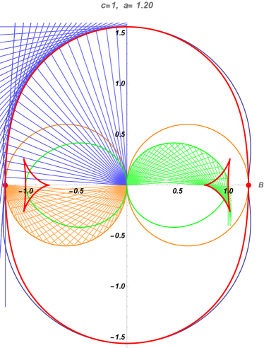
Figure 2: Left: Polar diagram illustrating the shape of fast and slow MHD pulses, evolving according to their group velocities, assuming the magnetic field is oriented in the $x$-direction. The fast wave expands in all directions, whilst the slow wave is restricted to a narrow sector about the field direction. As in the left frame of Figure 1, $c=10$, $a=9$ is assumed here, for which the cusp speed is $c_{\scriptscriptstyle T}=6.69$. Right: geometrical construction of a group speed polar diagram. See text for details.

For the magneto-acoustic waves, the group velocity is most easily calculated by introducing the notation $D(\omega,\mathbf{k})$ for their dispersion function, the second factor in Equation (27), and differentiating implicitly to get $(\partial D/\partial\omega)\,\partial\omega/\partial\mathbf{k}+\partial D/\partial\mathbf{k}=0$ by the chain rule, or

$$\frac{\partial\omega}{\partial\mathbf{k}}=-\frac{\partial D/\partial\mathbf{k}}{\partial D/\partial\omega}.$$ (34)

Specifically, the group speed parallel to the magnetic field is then

$$\frac{\partial\omega}{\partial k_{\scriptscriptstyle\parallel}}=\frac{(\omega^{4}-a^{2}c^{2}k^{4})k_{\scriptscriptstyle\parallel}}{\omega k^{2}[2\omega^{2}-(a^{2}+c^{2})k^{2}]},$$ (35)

and the perpendicular speed is

$$\frac{\partial\omega}{\partial k_{\scriptscriptstyle\!\perp}}=\frac{\omega^{3}k_{\scriptscriptstyle\!\perp}}{k^{2}[2\omega^{2}-(a^{2}+c^{2})k^{2}]},$$ (36)

where $k_{\scriptscriptstyle\!\perp}$ is the component of $\mathbf{k}$ perpendicular to ${\mathbf{B}}_{0}$. There is no energy propagation in the direction perpendicular to both ${\mathbf{B}}_{0}$ and $\mathbf{k}$.

A little algebra reveals that the group velocity of a fast wave propagating in the $\hat{\mathbf{B}}_{0}$ direction is the same as its phase velocity, $\max(a,c)\,\hat{\mathbf{B}}_{0}$, and similarly when propagating perpendicularly it is $\sqrt{a^{2}+c^{2}}\,\hat{\mathbf{k}}$. For intermediate directions, the group and phase speeds differ, as is clear from Figure 2.

The slow wave is even less isotropic. For parallel propagation its group velocity is $c_{\scriptscriptstyle T}\,\hat{\mathbf{B}}_{0}$, where $c_{\scriptscriptstyle T}=a\,c/\sqrt{a^{2}+c^{2}}$ is the so-called cusp speed, for reasons obvious from Figure 2.

Figure 2 (left panel) represents the shapes of the disturbed regions resulting from an MHD pulse emitted from the origin. The outermost wave front propagates at the group velocity. Depending on whether it was a fast wave pulse or a slow wave pulse, the two displayed shapes evolve. The shapes of these regions, especially for the slow wave, may be made clearer by geometric construction (right panel). Starting with the phase velocity polar diagram (blue for fast, orange for Alfvén, green for slow), draw a straight line from the origin to the phase locus. This is $\mathbf{k}$. From there, draw the perpendicular from that line; this represents the constant phase surfaces (perpendicular to $\mathbf{k}$). Do this for a large number of directions. You will notice, that these surfaces form envelopes. They are the group-velocity loci. The mysterious slow wave cusp is now easier to understand. Notice in particular that the lower half of the slow wave cusp is constructed from wave vectors oriented in the upward directions (green lines as drawn). That is, the phase and group velocities are directed on opposite sides of the $\hat{\mathbf{B}}_{0}$ direction, which may be verified algebraically using Equation (36) since the denominator is negative for the slow wave.

For the Alfvén wave, the group locus degenerates to a single point (the red dot) due to the well-known property of circles that an inscribed triangle with one side forming the diameter is a right-angled triangle.

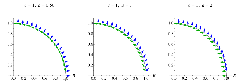
Figure 3: Velocity polarization directions of the slow (green) and fast (blue) waves for $a/c=0.5$ (left), 1 (centre) and 2 (right). The positions of the arrows correspond to the directions of the wave vector $\mathbf{k}$.

4 Wave Polarizations

It remains to emphasise the velocity polarizations of the three wave types. These are the eigenvectors $\mathbf{V}$ of the real symmetric matrix $A$ defined in Equation (30), and so they are necessarily orthogonal. The Alfvén wave is the simplest; it is polarized in the direction $\mathbf{k}{\boldsymbol{\times}}{\mathbf{B}}_{0}$, perpendicular to both $\mathbf{k}$ and ${\mathbf{B}}_{0}$. The fast and slow wave velocities therefore both lie in the plane spanned by those two vectors. Their directions are illustrated in Figure 3 for three ratios of the Alfvén to sound speeds. It is easily verified that the fast-wave polarization is longitudinal (i.e., in the $\mathbf{k}$ direction) for $a\ll c$, where it is essentially just the sound wave. The slow wave is therefore transverse to $\mathbf{k}$ in this limit. On the other hand, for $a\gg c$, the slow wave is just a field-guided sound wave restricted to have its velocity along ${\mathbf{B}}_{0}$, and so the fast wave is asymptotically transverse to the magnetic field. These considerations are very useful in understanding MHD waves in stratified atmospheres, where polarizations vary with height.

5 Waves in Stratified Atmospheres

Having introduced the basic MHD waves in a uniform plasma in Section 4, we now turn to the main topic of this chapter. How are these modified, or indeed do they even exist, in a continuously varying or stratified atmosphere like the solar chromosphere?

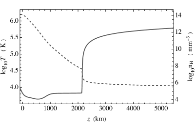
Figure 4: The temperature (full curve, left axis) and total hydrogen number density (dashed curve, right axis) plotted logarithmically as functions of height $z$ (km) in the mean quiet Sun Model C7 of AvrLoe08aa. The transition region around 2200 km presents a formidable barrier to waves attempting to enter the corona from below.

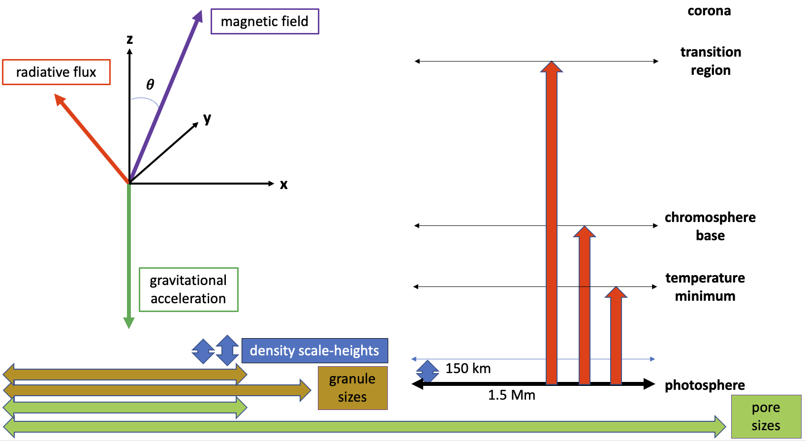
Figure 5: Schematic illustrating representative widths and heights in the solar atmosphere. The shorter and longer arrows corresponding to granules and pores indicate size ranges. The axes and arrows at top left indicate symmetry-breaking features that may cause MHD wave modes to interact.

Typically, the (mean) chromosphere is around 14 density scale-heights thick (see Figure 4), so gravitational stratification exerts a powerful influence on any waves. Figure 5 illustrates the extent to which vertical stratification dominates the low atmosphere. Even ‘tiny’ features such as pores and granules are many times wider than their density scale height at the photosphere, making gravitational stratification the dominant feature affecting wave propagation. Stratified atmospheres will be our main topic for the rest of this chapter.

1 Acoustic-Gravity Waves and the WKBJ Method

Before moving to MHD waves in stratified atmospheres, it is useful to explore the effects of stratification without the magnetic field. The two remaining restoring forces are buoyancy and gas pressure via compression.

Following DeuGou84aa, introducing $\psi=\rho^{1/2}c^{2}\mbox{\boldmath$\nabla$}{\boldsymbol{\cdot}}\hskip 1.5pt\mbox{\boldmath$\xi$}$ based on a method of Lam32aa, the linearized oscillation equations can be reduced to a single second-order normal-form ordinary differential equation (ODE) for the amplitude $\Psi(z)$, where $\psi(x,y,z,t)=\Psi(z)\exp[i(k_{x}x+k_{y}y-\omega t)]$:

$$\frac{\mathrm{d}^{2}\Psi}{\mathrm{d}z^{2}}=Q(z)\Psi,$$ (37)

where

$$Q(z)=k_{h}^{2}-\frac{\omega^{2}-\omega_{c}^{2}}{c^{2}}-\frac{N^{2}}{\omega^{2}}k_{h}^{2},$$ (38)

and

$$\omega_{c}^{2}=\frac{c^{2}}{4H^{2}}\left(1-2H^{\prime}\right)$$ (39)

is the square of the (or more properly an) acoustic cutoff frequency, $H_{\rho}=H=-\rho/\rho^{\prime}$ is the density scale height, $N^{2}=g/H-g^{2}/c^{2}$ is the square of the Brunt-Väisälä (buoyancy) frequency, and $k_{h}^{2}=k_{x}^{2}+k_{y}^{2}$ is the squared horizontal wavenumber.

Here ${}^{\prime}=d/dz$, and all equilibrium quantities may generally depend upon the vertical coordinate, $z$. The translational invariance in time and the two horizontal coordinates have been exploited to reduce the PDEs to ODEs in $z$. In place of the dispersion relation, or the inversion of a $3\times 3$ matrix, one is faced with solving a linear second-order ODE with three (possibly) complex parameters $\omega,k_{x},k_{y}$. When $\Psi$ is determined, $\psi(x,y,z,t)$ is again obtained by inverting three Fourier transforms. As before, we have for convenience suppressed a source term, which depends upon the three complex Fourier variables and $z$, in Equation (37), to avoid the trivial solution $\Psi=0$. The solution of the resulting inhomogeneous equation must necessarily include the Wronskian of the two linearly-independent solutions.

A wave-energy/flux conservation law also holds for acoustic-gravity waves. The appropriate expressions are now U_2 = 12 ρ_0 v^2 + p122ρ0c2 + ρ0N22 ( η1η0’ )^2 ,
f_2 = p_1 v. Notice that acoustic-gravity waves generally have non-zero (Eulerian) entropy fluctuations. The Lagrangian (comoving) entropy fluctuation is exactly zero. For an isentropic stratified atmosphere (i.e., $\eta_{0}^{\prime}=N^{2}=0$), the third term (thermobaric energy density) in the expression for the energy density is absent: both Lagrangian and Eulerian entropy fluctuations vanish.

In the case of an isothermal atmosphere, where $c$, $H=c^{2}/(\gamma g)$ and $N^{2}=(\gamma-1)g^{2}/c^{2}$ are all constant, Equation (37) may be solved exactly in terms of elementary functions, $\Psi_{\mbox{\scriptsize iso}}\propto\exp(\pm ik_{z}z)$, where:

$$k_{z}^{2}=\frac{\omega^{2}-\omega_{c}^{2}}{c^{2}}+\frac{N^{2}}{\omega^{2}}k_{h}^{2}-k_{h}^{2}.$$ (40)

Waves are therefore travelling vertically (or standing) if $k_{z}^{2}>0$ and evanescent if $k_{z}^{2}<0$. Arbitrarily setting $k_{y}=0$, $k_{h}=k_{x}$, Figure 6 partitions the $k_{x}$–$\omega$ plane into travelling (Region I and II) and evanescent (III and IV) regions. A dimensionless wavenumber $\kappa=k_{x}H$ and frequency $\nu=\omega H/c$ are used. The dimensionless acoustic cutoff frequency in these units is exactly ${\textstyle\frac{1}{2}}$. Region I, which is entirely above this cutoff, hosts acoustic waves somewhat modified by gravity, progressively less so as frequency increases. Region II, which is entirely below both the cutoff and Brunt-Väisälä frequencies, hosts internal gravity waves somewhat modified by acoustic effects.

A semi-infinite isothermal atmosphere provides a boundary along which an evanescent (Region III and IV) acoustic-gravity wave may propagate. The Lamb wave ($\omega^{2}=k_{h}^{2}c^{2}$) lives in an atmosphere with a rigid lower boundary, like the Earth’s atmosphere. The surface gravity wave, or f-mode ($\omega^{2}=gk_{h}$), lives in an atmosphere with a stress-free upper boundary, like a stellar convective envelope.

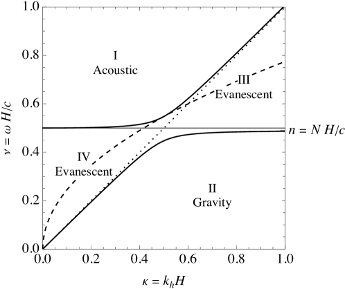
Figure 6: Regions of the $k_{x}-\omega$ plane inhabited by modified acoustic, modified gravity, and evanescent waves. This diagram is calculated for an isothermal atmosphere, but will be similar for more general cases. Region I corresponds to vertically propagating acoustic waves, Region II to propagating gravity waves, and Regions III and IV to evanescent waves. The dotted line is the Lamb wave $\nu=\kappa$ and the dashed curve is the f-mode $\nu^{2}=\kappa/\gamma$. For the case $\gamma=5/3$.

Returning to the more general (non-isothermal) case, exact solutions may, or may not, exist in terms of standard tabulated special functions. As this equation is equivalent to the standard one-dimensional time-independent Schrödinger equation with a potential $Q(z)$, there exist tabulations of $Q$s for which the equation yields familiar special functions. Their Wronskians and dispersion relations are readily computed.

The analytic properties of $Q(z)$, with $z$ taken to be a complex variable, determine the singular points of the ODE, and enable one to classify the ODE and obtain Frobenius and asymptotic expansions valid in the neighborhoods of the singular points. Numerical methods may be employed between the singular points to connect the linearly-independent solutions around the singular points.

The eikonal or WKBJ method (BenOrs78aa) yields a high-frequency asymptotic-solution. For example, if $Q(z)<0$ throughout, corresponding to Region I or II in the isothermal case, an upward ($+$ sign) or downward ($-$ sign) travelling wave would satisfy

$$\Psi\sim C\left[-Q(z)\right]^{-1/4}\exp\left[\pm i\!\int^{z}\sqrt{-Q(z^{\prime})}\,dz^{\prime}\right]$$ (41)

as $|Q|\,H^{2}\to\infty$, which in effect can mean $\omega\to\infty$ in Region I or $\omega\to 0$ in Region II. Similarly if $Q(z)>0$ throughout, the upwardly evanescent wave is represented asymptotically by

$$\Psi\sim C\,Q(z)^{-1/4}\exp\left[-\int^{z}\sqrt{Q(z^{\prime})}\,dz^{\prime}\right].$$ (42)

These eikonal asymptotic formulae do not apply near a turning point $z_{t}$ (corresponding to the boundaries of Regions I and II in figure 6) at which $Q(z)=0$ with $Q^{\prime}(z_{t})>0$. However, the distinguishing feature of the WKBJ method that elevates it beyond the simple eikonal method is that a matching across $z_{t}$ can be developed that is valid uniformly across the domain (the Langer solution; BenOrs78aa):

$$\Psi(z)\sim C\,\left(\frac{3}{2}S_{0}(z)\right)^{1/6}Q(z)^{-1/4}\mathop{\rm Ai}\nolimits\left[\left(\frac{3}{2}S_{0}(z)\right)^{2/3}\right],$$ (43)

where $S_{0}(z)=\int_{z_{t}}^{z}\sqrt{Q(z^{\prime})\,dz^{\prime}}$, $C$ is a normalization constant and $\mathop{\rm Ai}\nolimits$ is the Airy function of the first kind. This is useful in modelling the effect of the acoustic cutoff in confining low frequency ($\,\lesssim 5$ mHz) solar p-modes. (It is assumed that $z_{t}$ is a simple isolated zero of $Q$.) Care must be taken with Equation (43) because of the fractional powers and $S_{0}$ being imaginary on $z<z_{t}$. Specifically, on $z<z_{t}$ one must select $\arg S_{0}=3\pi/2$, so that $\arg S_{0}^{1/6}=\pi/4$ and $\arg S_{0}^{2/3}=\pi$. The principal real positive root applies on $z>z_{t}$.

Of course, the exact location of the turning point of a wave, identified here with $Q=0$ and hence with an inflection point $\Psi^{\prime\prime}=0$, depends crucially on the choice of dependent and independent variables used to express the wave equation. Different choices lead to different expressions for the cutoff frequency (SchFle98aa; SchFle03aa), though the Brunt-Väisälä frequency is not affected. This makes it difficult to interpret observations in terms of a height-dependent cutoff frequency. In addition, formulae such as (39) that involve higher derivatives, in this case the second $z$-derivative of the density, produce very spiky cutoff frequency profiles when applied to tabulated empirical atmosphere models such as the widely used Model C of VerAvrLoe81aa (the VAL C model). This complicates both interpretation and numerical modelling using, in particular, ray theory.

The acoustic cutoff, and how it is modified by magnetic field, plays an important role in the propagation of waves through the solar chromosphere, as explored in Section 3.

2 MAG Waves

The generalization of Section 4 to an arbitrarily-stratified stationary magneto-atmosphere is straightforward. ∂ρ1∂t+$\nabla$⋅ ρ_0 v=0,
ρ_0∂v∂t=-$\nabla$p_1+ρ_1g_0 + 1μ($\nabla$× B_0)× B_1 + 1μ($\nabla$× B_1)× B_0,
Dp1Dt-c^2Dρ1Dt= (γ-1) ρ_0 T_0 Dη1Dt = 0,
∂B1∂t=$\nabla$×(v ×B_0),
$\nabla$⋅ B_1=0. By assumption, the equilibrium quantities satisfy the three MHS constraints:

$$0=-\mbox{\boldmath$\nabla$}p_{0}+\rho_{0}\,{\mathbf{g}}_{0}+\frac{1}{\mu}\left(\mbox{\boldmath$\nabla$}{\boldsymbol{\times}}\hskip 1.5pt{\mathbf{B}}_{0}\right){\boldsymbol{\times}}\,{\mathbf{B}}_{0},$$ (44)

and $\mbox{\boldmath$\nabla$}{\boldsymbol{\cdot}}\hskip 1.5pt{\mathbf{B}}_{0}=0$.

The neglect of the term $\rho_{0}{\mathbf{g}}_{1}$ in the linearized equations is known as the Cowling approximation. It is extremely accurate in most situations. Accordingly, we may simply set ${\mathbf{g}}_{0}={\mathbf{g}}$. The adiabatic sound speed $c$ (and the Alfvén speed $a$) is also derived from the equilibrium pressure, density, and ratio of specific heats. It may depend upon all three spatial coordinates. All dissipative (i.e., non-ideal) terms have been omitted from these equations.

As before, it proves possible to reduce these to a single vector wave-equation for $\bf v$: ∂2v∂t2= 1ρ0 $\nabla$( ρ_0 c^2$\nabla$⋅ v) + $\nabla$(v⋅g) - g($\nabla$⋅ v) +1μρ0 ($\nabla$×($\nabla$×(v×B_0)))​×B_0
+ 1μρ0 $\nabla$( v⋅( $\nabla$×B_0 ) ) + 1μρ0 ( ( $\nabla$×B_0 ) ×( $\nabla$×( v×B_0 ) ) ) ≡- G[v], a result which was first derived by FerPlu58aa. This result is exact given our assumptions. It describes not only MAG waves that propagate through stable equilibria, but it will also capture the ideal instabilities (see Section 2).

A wave-energy/flux conservation law may again be deduced from this set of linearized equations. It is the obvious hybrid obtained by combining the previous results for the acoustic-gravity and MHD waves.

3 Exact 2D MHD Solutions and their Mixed Properties

Exact solutions in any form of modelling have value beyond their strict applicability to reality. They help us understand processes and possibilities, and also provide rigorous tests for numerical schemes. The combination of all three restoring forces – gas pressure, buoyancy and Lorentz force – in a non-trivial exact solution obtained by ZhuDzh84aa was therefore a most welcome, if unexpected, innovation.

Their model is of ideal MHD waves in a plane-stratified isothermal atmosphere with uniform non-horizontal magnetic field in the two-dimensional (2D) case in which the gravitational acceleration, magnetic field and direction of wave propagation are all co-planar (in the $x$–$z$ plane for example). In $(x,y,z)$ Cartesian coordinates, we set the background magnetic field to ${\mathbf{B}}_{0}=B_{0}(\sin\theta,0,\cos\theta)$, where $\theta$ is the inclination angle of the field relative to the vertical (see Figure 5).

Before describing this exact solution in the remainder of this section, we pause to make a few contextual remarks. By exact solutions for MAG waves we mean solutions where the analogous $\Psi$s are given in terms of tabulated special functions. There are many such exact solutions in the literature. Virtually all of these pertain to an equilibrium where the magnetic field is everywhere perpendicular to the gravitational acceleration and the atmospheric stratification. Such a configuration admittedly constitutes a set of measure zero when compared with all the possible directions a magnetic field may point. Moreover, this case is also singular in the sense that neither the mathematical methods nor physical outcomes follow uniformly from the $\theta\to\pi/2$ limit of the ZhuDzh84aa exact solution, where the governing differential equation reduces from fourth order to second order, with attendant perplexing introduction of horizontal critical layers. In these layers wave energy-fluxes may be discontinuous (a process unfortunately called ‘resonant absorption’) and some components of the wave motion are unbounded, or diverge as one approaches the layer from above or below. Steep gradients develop. The divergence of a wave amplitude is, of course, entirely at odds with the linearization procedure. Some authors invoke finite dissipation to limit spatial gradients, suppress divergences, and provide a physical basis for the resonant absorption. Such a ‘renormalization’ of an infinity is not unreasonable. Yet, it leaves several fundamental questions unanswered. The horizontal field case is discussed briefly in Section LABEL:sec:horiz.

The $\theta\rightarrow\pi/2$ limit of Zhugzhda and Dzhalilov’s exact solution is particularly valuable in providing the correct physical interpretation of the singular mathematical behavior of these horizontal magnetic field MAG wave solutions. This limit also answers the useful question as to just how inclined a magnetic field needs to be in order that it is effectively horizontal.

For all these reasons we devote this section to the remarkable exact solution of ZhuDzh84aa despite, as shall presently become clear, the significant amount of algebra and special-function gymnastics involved.

In terms of the component of plasma velocity $u_{\scriptscriptstyle\!\perp}$ perpendicular to the background magnetic field (lying in the $x$–$z$ plane), the linearized MHD equations may be combined into a single fourth-order ODE best couched in terms of dimensionless versions of parameters familiar from the above acoustic-gravity solution.

First, introduce the independent position variable $s=\omega H/a$ in terms of the wave circular frequency $\omega$, density scale height $H$ and Alfvén speed $a(z)=a_{0}\exp[z/2H]$; the dimensionless frequency $\nu=\omega H/c$; the dimensionless Brunt-Väisälä frequency $n=NH/c$; and the dimensionless horizontal wavenumber $\kappa=k_{x}H$. Note that $s$ increases downward, from $s=0$ at $z=+\infty$ to $s=\infty$ at $z=-\infty$. We then introduce the dimensionless vertical wavenumber from the acoustic-gravity dispersion relation Equation (40),

$$\kappa_{z}=\sqrt{\nu^{2}-\kappa^{2}+n^{2}\kappa^{2}/\nu^{2}-{\textstyle\frac{1}{4}}},$$ (45)

where it should be noted that the ${\textstyle\frac{1}{4}}$ is the square of the acoustic cutoff frequency in these units. Finally, we define $\kappa_{0}=\sqrt{\nu^{2}\sec^{2}\theta-\frac{1}{4}}$, the significance of which will become clear shortly.

The perturbed variables in the linearized MHD equations may all be eliminated in favour of $u_{\scriptscriptstyle\!\perp}$, resulting in a linear homogeneous fourth-order ODE (see ZhuDzh84aa, for both a statement of the DE and solutions in terms of Meijer G-functions) u_​⟂^(4) s ^4+4 secθ(cosθ-i κsinθ) u_​⟂^(3) s ^3
+2 sec^2θ[(2 κ_0^2+1) cos^2θ-4 i κsinθcosθ+2 (s ^2-κ^2)] u_​⟂” s ^2
+4 sec^2θ[4  i   κ^3cosθsinθ-κ^2+3 s ^2+cos^2θ(2 κ^2+κ_0^2)] u_​⟂’ s
+4 sec^2θ[4 κ^4-4  i cosθsinθ  κ^3-cos^2θ(4 κ^2+4 κ_0^2+1) κ^2+s ^2 (4 κ_z^2+1)] u_​⟂
=0. As in our previous cases, we have once again omitted writing out the explicit expression of the source term that should appear on the right side of this equation.

This equation, while daunting in appearance, is actually amenable to an analytic treatment. One begins by noting that this equation has two singular points: a regular singularity at the origin ($s=0$) and an irregular singularity at infinity ($1/s=0$). In a neighborhood of the former, the method of Frobenius may be applied to determine four linearly-independent power-series solutions. Alternatively, the fourth-order differential equation can be written in a standard form known to admit hypergeometric solutions.

Cal01aa for vertical magnetic field and HanCal09aa for the general case recognized that these four solutions may be expressed most simply in terms of the ${}_{2}F_{3}$ generalized hypergeometric function,

$${}_{2}F_{3}(a_{1},\,a_{2};\,b_{1},\,b_{2},\,b_{3};\,x)=\sum_{n=0}^{\infty}\frac{(a_{1})_{n}\,(a_{2})_{n}}{(b_{1})_{n}\,(b_{2})_{n}\,(b_{3})_{n}}\,\frac{x^{n}}{n!}\,,$$ (46)

where $(a)_{0}=1$, $(a)_{n}=a(a+1)\ldots(a+n-1)$ is the Pochhammer symbol. These functions are entire. Specifically, they found

$$\split u_{\scriptscriptstyle\!\perp}=&C_{1}\,u_{1}+C_{2}\,u_{2}+C_{3}\,u_{3}+C_{4}\,u_{4}\\ =C_{1}\,s^{-2\kappa}\,{}_{2}F_{3}\bigl{(}\textstyle{\textstyle\frac{1}{2}}-\kappa-i\kappa_{z},\,{\textstyle\frac{1}{2}}-\kappa+i\kappa_{z};\\ \qquad\quad\,1-2\kappa,\,{\textstyle\frac{1}{2}}-\kappa-{i}\kappa_{0}-{i}\kappa\tan\theta,\,{\textstyle\frac{1}{2}}-\kappa+{i}\kappa_{0}-{i}\kappa\tan\theta;\,-s^{2}\sec^{2}\theta\bigr{)}\\ +C_{2}\,s^{2\kappa}\,{}_{2}F_{3}\bigl{(}\textstyle{\textstyle\frac{1}{2}}+\kappa-i\kappa_{z},\,{\textstyle\frac{1}{2}}+\kappa+i\kappa_{z};\\ \qquad\quad\,1+2\kappa,\,{\textstyle\frac{1}{2}}+\kappa-{i}\kappa_{0}-i\kappa\tan\theta,\,{\textstyle\frac{1}{2}}+\kappa+{i}\kappa_{0}-{i}\kappa\tan\theta;\,-s^{2}\sec^{2}\theta\bigr{)}\\ +C_{3}\,s^{1-2{i}\kappa_{0}+2{i}\kappa\tan\theta}\,{}_{2}F_{3}\bigl{(}\textstyle 1-{i}\kappa_{0}-i\kappa_{z}+{i}\kappa\tan\theta,\,1-{i}\kappa_{0}+i\kappa_{z}+{i}\kappa\tan\theta;\\ \qquad\quad\,1-2i\kappa_{0},\,{\textstyle\frac{3}{2}}-{i}\kappa_{0}-\kappa+{i}\kappa\tan\theta,\,{\textstyle\frac{3}{2}}-{i}\kappa_{0}+\kappa+{i}\kappa\tan\theta;\,-s^{2}\sec^{2}\theta\bigr{)}\\ +C_{4}\,s^{1+2{i}\kappa_{0}+2{i}\kappa\tan\theta}\,{}_{2}F_{3}\bigl{(}\textstyle 1+{i}\kappa_{0}-i\kappa_{z}+i\kappa\tan\theta,\,1+{i}\kappa_{0}+i\kappa_{z}+{i}\kappa\tan\theta;\\ \qquad\quad\,1+2{i}\kappa_{0},\,{\textstyle\frac{3}{2}}+{i}\kappa_{0}-\kappa+{i}\kappa\tan\theta,\,{\textstyle\frac{3}{2}}+{i}\kappa_{0}+\kappa+{i}\kappa\tan\theta;\,-s^{2}\sec^{2}\theta\bigr{)}\,,$$ (47)

where the $C_{i}$ are four arbitrary amplitudes. As the ${}_{2}F_{3}$ power series all tend to 1 as $s\to 0$, the behavior of each solution for small $s$ is determined by the power of $s$ multiplying the hypergeometric function in each expression.

The solutions $u_{1}$ and $u_{2}$ are paired. They describe a single MAG wave mode with opposite directions of propagation (toward or away from $s=0$). Likewise, $u_{3}$ and $u_{4}$ pair to describe a second distinct MAG wave mode. These two wave modes are asymptotic to the fast and slow MHD waves, respectively, in the WKBJ limit. The direction of propagation is determined by the sign convention chosen for the Fourier transforms in $t$ and $x$. In other words, $u_{\scriptscriptstyle\!\perp}$ is multiplied by a factor $\exp[\pm i(k_{x}x\pm\omega t)]$ in calculating the inverse Fourier transform with a definite choice for each $\pm$. We adopt $\exp[i(k_{x}x-\omega t)]$ throughout. Typically, one member of each pair is dropped because it leads to an acausal or unphysical solution in the neighborhood of $s=0$.

The family of generalized hypergeometric functions, ${}_{p}F_{q}(\{a_{i}\},\{b_{j}\};x)$ includes most of the familiar special functions of mathematical physics, for example, the exponential ($p=q=0$), Bessel ($p=0,q=1$), Whittaker ($p=q=1$), and Legendre ($p=2,q=1$), functions. When $p$ is less than or equal to $q$, as obtains above, then the power series is absolutely convergent for all finite values of s. (Otherwise, $x=1$ is a third regular singularity, and the power series converge only for $|x|$ less than one.) What is especially valuable about this family of functions is that each power series may be expressed as a contour integral. This in turn may be used to determine the asymptotic behavior of the power series in the neighborhood of the irregular singular point $1/s=0$. In other words, one obtains the asymptotic behavior of a given power series as a linear combination of the four linearly-independent solutions valid in the neighborhood of the irregular singular point at infinity!

Analytic expressions for the four coefficients – expressed in terms of the coefficients $\{a_{i}\}$ and $\{b_{j}\}$ – are conveniently provided by Luk75aa. Let $U_{j}$ for $j=1,2,3,4$ be the four linearly-independent solutions in the neighborhood of $1/s=0$, then for each $i=1,2,3,4$ we have $u_{i}=a_{ji}U_{j}$ with summation convention implied, i.e.,

$$u_{i}=a_{1i}\,U_{1}+a_{2i}\,U_{2}+a_{3i}\,U_{3}+a_{4i}\,U_{4},$$ (48)

where the sixteen $a_{ji}$ are known in terms of $\kappa$, $\kappa_{0}$, $\kappa_{z}$ and $\theta$ and are independent of $s$. All sixteen are set out in Table 1 of HanCalDon16aa, and involve nothing more complicated than gamma and trigonometric functions.

Because $1/s=0$ is an irregular singular point of the ODE, the expressions for the $U_{j}$ are formally divergent infinite series which are asymptotically exact as $s\rightarrow\infty$. This behavior is entirely analogous to the asymptotic expressions for the Hankel functions $H_{\nu}^{(1)}(x)$ and $H_{\nu}^{(2)}(x)$ as $x\rightarrow\infty$, i.e.,

$$H_{\nu}^{(1,2)}(x)\sim\sqrt{\frac{2}{\pi x}}\exp\left[\pm{i}\left(x-\frac{\nu\pi}{2}-\frac{\pi}{4}\right)\right].$$ (49)

In the present circumstances each of the four hypergeometric solutions with Frobenius solutions centred at $s=0$ connects to four asymptotic behaviours (NIST:DLMF, Equation (16.11.8)) u