A stable homotopy invariant for Legendrians with generating families

Abstract.

We construct a stable homotopy type invariant for any Legendrian submanifold in a jet bundle equipped with a linear-at-infinity generating family. We show that this spectrum lifts the generating family homology groups. When the generating family extends to a generating family for an embedded Lagrangian filling, we lift the Seidel isomorphism to the spectrum level. As applications, we establish topological constraints on Lagrangian fillings arising from generating families, algebraic constraints on whether generating families admit fillings, and lower bounds on how many fiber dimensions are needed to construct a generating family for a Legendrian.

1. Introduction

A central problem in contact topology is the search for invariants of Legendrian submanifolds of contact manifolds. Given $\mathbb{R}^{2n+1}$ with its standard contact structure $\xi_{0}=\ker(dz-y\,dx)$, there are classical integer-valued invariants of a closed Legendrian $\Lambda\subset\mathbb{R}^{2n+1}$ known as the Thurston-Bennequin and rotation numbers; for definitions, see [15]. For a Legendrian with vanishing rotation number, there exist categorifications: homological invariants of the Legendrian that can recover the Thurston-Bennequin number; [7, Proposition 5.7], [15, Proposition 3.3].

Indeed, given a Legendrian $\Lambda$ with an augmentation $\epsilon$, it is possible to define linearized contact homology $LCH_{*}(\Lambda,\epsilon;R)$ [7, 14, 26] via the theory of holomorphic curves. When $\Lambda$ is equipped with a generating family $f$, building on work in [49, 51], Fuchs and Rutherford [18] defined generating family homology, $GFH_{*}(\Lambda,f;R)$. For both these homology theories $R$ denotes a ring of coefficients. It has been established [18] that for a $1$-dimensional Legendrian the existence of a linear-at-infinity $f$ implies the existence of an augmentation $\epsilon_{f}$ and an isomorphism

(1.1) $$GFH_{*+c}(\Lambda,f;\mathbb{Z}/2\mathbb{Z})\cong LCH_{*}(\Lambda,\epsilon_{f};\mathbb{Z}/2\mathbb{Z}).$$

Here, $c$ is a constant equalling either 0 or 1 depending on the convention. In this and further work, we will employ the convention that $c=1$ (see Remark 1.31 and Remark 3.10). The $c=0$ convention will only appear briefly in Section 3.4, with explicit notation indicating the convention shift.

Homological invariants can admit stable homotopy refinements. In homotopy theory, the stable homotopy type of a space is a refinement of the singular chain complex of the space. In low-dimensional topology, Lipshitz and Sarkar [30] showed that the chain complex underlying Khovanov homology has a refinement to a CW spectrum. These spectra have homology groups that recover Khovanov homology and contain more information: By studying Steenrod operations, Seed [44] found examples of smooth knots with the same Khovanov homology but nonequivalent spectra. In the realm of geometric invariants constructed from Floer theory, Floer noted in their original works [17] that stable homotopy refinements of Floer homology groups should be present. Since then, many stable homotopy types lifting Floer-type homology groups have been constructed. In symplectic geometry, Cohen-Jones-Segal outlined an approach using flow categories [10], Kragh lifted both symplectic homology and Viterbo’s transfer maps [27], and Abouzaid-Blumberg have lifted Hamiltonian Floer homology [1]. In Seiberg-Witten theory, one has Bauer-Furuta’s invariants [3] and Manolescu’s equivariant stable homotopy type [33]. Forthcoming work of Lazarev is expected to produce spectral lifts of Floer cohomology between the zero section and a Lagrangian in a cotangent bundle, via generating families.

Riding this progression of finer and finer invariants, it is natural to ask:

Question 1.1.

Are there spectral lifts of linearized contact homology or of generating family homology?

For linearized contact homology, the answer is widely expected to be yes under favorable circumstances, and the (still open) construction of such a lift falls under the purview of an active field, often called Floer homotopy theory. For generating family homology, we provide an affirmative answer in this work. More precisely, fix a smooth manifold $B$, a closed Legendrian $\Lambda\subset J^{1}B$ in the $1$-jet bundle of $B$, and a linear-at-infinity generating family

$$f:B\times\mathbb{R}^{N}\to\mathbb{R}$$

for $\Lambda$ (see Definition 2.13). From this data we define a stable homotopy type (Definition 3.1)

(1.2) $$C(\Lambda,f;\mathbb{S})$$

that we call the generating family spectrum associated to the pair $(\Lambda,f)$. We prove that our spectral lifts are invariants of the pair $(\Lambda,f)$ (Theorem 1.2) and that the spectrum recovers generating family homology (Theorem 1.4). We also establish a highly useful structural result: The Seidel isomorphism lifts to stable homotopy (Theorem 1.12).

1.1. Main results

Theorem 1.2 (Proposition 3.6 and Theorem 3.7.).

The generating family spectrum of $(\Lambda,f)$ is invariant under Legendrian isotopy and equivalence of generating families (Definition 2.4).

Remark 1.3.

$C(\Lambda,f;\mathbb{S})$ is an invariant not of $\Lambda$ alone, but of the pair $(\Lambda,f)$. One expects that the (Spanier-Whitehead duals to) the collection of spectra $\{C(\Lambda,f;\mathbb{S})\}_{f}$ form endomorphisms in a non-unital $\infty$-category associated to $\Lambda$ – see Section 1.4.

The following is proven in Section 3.4. See Definition 3.8 for the definition of $GFH$ and for an explicit description of the grading convention used in this work.

Theorem 1.4.

The generating family spectrum is a lift of generating family homology. That is, for any coefficient abelian group $A$, the generating family homology of $(\Lambda,f)$ is isomorphic to the homology of the generating family spectrum:

$$\forall k\in\mathbb{Z},\qquad H_{k}(C(\Lambda,f;\mathbb{S});A)\cong{GFH}_{k}(\Lambda,f;A).$$

Remark 1.5.

Theorem 1.4 in part explains the appearance of the sphere spectrum $\mathbb{S}$ in our notation. Indeed, the notation (1.2) is meant to evoke “generating family chains with coefficients in the sphere spectrum.” We view classical $GFH$ as a linear invariant computed using $\mathbb{Z}$-linear coefficients, while the generating family spectrum is a lift to sphere-spectrum-linear coefficients.

Generating families pose interesting geometric questions of their own. For example, given a Legendrian $\Lambda$ equipped with a linear-at-infinity generating family $f:B\times\mathbb{R}^{N}\to\mathbb{R}$, one can define the dimension of $f$, $\dim f$, to be the fiber dimension $N$, and ask to reduce $\dim f$. More precisely, let $[(\Lambda,f)]$ denote the equivalence class of $(\Lambda,f)$ generated by stabilization, fiber-wise diffeomorphism, and Legendrian isotopy (Section 2.2 and Proposition 2.28). We can ask: What is

$$N_{\min}[(\Lambda,f)]:=\min_{(\Lambda^{\prime},f^{\prime})\in[(\Lambda,f)]}\{\dim f^{\prime}\}?$$

For a fixed 1-dimensional Legendrian equipped with a graded, normal ruling, Fuchs and Rutherford gave an algorithm to construct a generating family that would induce this ruling [18, Section 3]. There is an algorithm to go from a generating family to a ruling, which can be found in [8] and [18, Section 2], and thus for a fixed pair $(\Lambda,f)$, the algorithms give an upper bound to $N_{\min}[(\Lambda,f)]$.

The next theorem shows that the generating family spectrum produces a lower bound on $N_{\min}[(\Lambda,f)]$. It is proven in Section 3.3.

Theorem 1.6.

Suppose $\Lambda\subset J^{1}B$, and let $N$ be the minimal non-negative integer for which $\Sigma^{N}C(\Lambda,f;\mathbb{S})$ is equivalent to a suspension spectrum – i.e., for which there exists a pointed space $A$ and an equivalence of spectra

$$C(\Lambda,f;\mathbb{S})\simeq\Sigma^{-N}(\Sigma^{\infty}(A)).$$

Then

$$N\leq N_{\min}[(\Lambda,f)].$$

In particular, $f$ itself cannot arise as a stabilization of an $(N-1)$-dimensional generating family.

We review the definition of suspension spectra in Definition C.11 of the Appendix.

The stable-homotopy bounds of Theorem 1.6 immediately give bounds using homology. In the following, and as we do throughout this work, we use the grading convention $c=1$ in (1.1) – i.e., the convention in Definition 3.8.

Corollary 1.7.

Fix a linear-at-infinity generating family $f$ for an $m$-dimensional connected Legendrian $\Lambda\subset J^{1}B$. Suppose, for some coefficient group, the generating family homology $GFH_{-k}(\Lambda,f)$ is non-zero for some $k\geq 0$. Suppose also that for some coefficient group (not necessarily equal to the previous coefficient group) $GFH_{\ell}(\Lambda,f)$ is non-zero for some $\ell\geq 0$. Then $N_{\min}\geq\max\{k+1,\ell-m\}$.

Proof.

Suppose $\Lambda\subset J^{1}B$ is an $m$-dimensional connected Legendrian. Because $\Lambda$ is connected, we may as well assume $B$ is connected. Given a generating family $f:B\times\mathbb{R}^{N}\to\mathbb{R}$ for $\Lambda$, the difference function has domain $B\times\mathbb{R}^{2N}$, so for any real number $\epsilon$, the associated sublevel quotient $B\times\mathbb{R}^{2N}/\{f\leq\epsilon\}$ is homotopy equivalent to some pointed CW complex $A$ with cells of dimension at most $2N+\dim B=2N+m$. By Definition 3.1, the generating family spectrum $C(\Lambda,f;\mathbb{S})$ is equivalent to $\Sigma^{-N}\Sigma^{\infty}A$ – the suspension spectrum of $A$, shifted $-N$ times (for $\epsilon$ positive and small enough). So the generating family spectrum is generated by spheres of at least degree $-N$ and at most degree $N+m$. In particular, generating family homology can only be non-zero in degrees between $-N$ and $N+m$, inclusive.

If $f$ is linear at infinity, the space $\{f\leq\epsilon\}\subset B\times\mathbb{R}^{2N}$ is non-empty. (See also Remark 2.15.) Because $\epsilon$ is a regular value of $f$ – combine Lemma 2.11, Proposition 2.21, and Choice 2.22 – it follows that the quotient space $A$ is path-connected. In particular, $A$ has reduced homology $\widetilde{H}_{0}(A)\cong 0$. Applying the shift by $-N$, we see that $GFH_{*}(\Lambda,f)\neq 0$ implies that $-N+1\leq*\leq N+m$. In particular, defining $k$ and $\ell$ as above, we see that $N\geq k+1$ and $N\geq\ell-m$. This shows $N_{\min}\geq\max\{k+1,\ell-m\}$. ∎

Remark 1.8.

If one chooses the coefficient group to be $\mathbb{Z}/2\mathbb{Z}$, then $GFH_{-k}(\Lambda,f)$ is non-zero if and only if $GFH_{m+1+k}(\Lambda,f)$ is non-zero by duality of $GFH_{*}(\Lambda,f)$ [5, Theorem 1.1]. In particular, $\ell-m=(m+1+k)-m=k+1$.

Remark 1.9.

We caution that duality does not hold for all $(\Lambda,f)$ in general with arbitrary coefficient groups for homology. For example, the statement of Theorem 6.1(1) [5] utilizes Poincaré duality for $\Lambda$, and indeed the proof relies on Lemma 7.1 of [42] which in turn utilizes Alexander/Lefschetz/Poincaré duality (which requires orientation hypotheses on $\Lambda$).

It is not hard to find a counter-example to duality if one violates orientation hypotheses. For example, take $B=\mathbb{R}P^{2n}$ and let $f:B\times\mathbb{R}\to\mathbb{R}$ be a cubic function, constant in the $B$-variable, with two critical points in each fiber of distinct critical values. Then $f$ generates a Legendrian $\Lambda\cong B\coprod B\subset J^{1}(B)$, and the generating family spectrum of $(\Lambda,f)$ is computed in Example 1.26 below. Because the homology of $\Sigma^{\infty}(B_{+})$ is the (unreduced) homology of $B$, incorporating the appropriate shifts, one finds (for any coefficient group):

$$GFH_{a}(\Lambda,f)\cong H_{a+1}(B)\qquad\forall a\in\mathbb{Z}.$$

Then over $\mathbb{Z}$ or over a finite field $\mathbb{F}_{p}$ with odd $p$, one can check that the extremal values of $k+1$ and $\ell-m$ do not agree.

Remark 1.10.

One can in fact prove Corollary 1.7 without ever knowing about generating family spectra – after all, one does not need to know about spectra to study (a shift of) the cellular chain complex. Note also that the corollary is a weaker conclusion than Theorem 1.6, since there exist spectra whose homology range behaves like a suspension spectrum’s, but which are not suspension spectra. One example is $X=\Sigma^{-1}\Sigma^{\infty}\mathbb{C}P^{N}$ for $N\geq 2$. Because the homology of $X$ is only non-zero in degrees $1,3,\ldots,2N-1$, its homology alone leaves open the possibility that $X$ is the suspension spectrum of a connected pointed CW complex – but $X$ cannot be a suspension spectrum because the Steenrod operation $Sq^{2}$ does not vanish on $H^{1}(X)\cong H^{2}(\mathbb{C}P^{N})$. This is one example of spectra harboring more information than chain complexes.

Example 1.11.

Consider the Legendrian knot $\Lambda\subset\mathbb{R}^{3}=J^{1}\mathbb{R}$ with its unique graded, normal ruling shown in Figure 1. By the algorithm in [18, Section 3], $\Lambda$ admits a generating family $f:\mathbb{R}\times\mathbb{R}^{N}\to\mathbb{R}$ with $N=9$ that will induce this ruling: for a graded ruling, assuming that the index at each switch is at least $2$, the algorithm produces a generating family with dimension equaling two greater than the maximum of the switch indices, which is $2+\max\{2,\dots,7\}=9$ in this example. Thus $N_{\min}[(\Lambda,f)]\leq 9$. Calculations of $LCH(\Lambda,\epsilon)$ from [36, Section 3] combined with (1.1) show that $GFH_{k}(\Lambda,f)$ is non-zero in degree $-4,0,6$ with our grading convention of $c=1$ – see Equation (1.1). Thus, by Corollary 1.7, $N_{\min}[(\Lambda,f)]\geq 5$. It is unknown whether this Legendrian admits a generating family $f$ with $\dim f=5$.

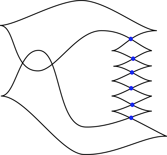
Figure 1. This Legendrian knot twist knot $\Lambda$ has a generating family $f$ corresponding to the ruling arising from switches at the $6$ marked crossings; the associated $GFH_{k}(\Lambda,f;\mathbb{Z})$ is non-zero in dimensions $-4,0$, and $6$, using our grading convention.

When a generating family $f$ for a Legendrian $\Lambda$ extends to a “tame” generating family $F$ for a Lagrangian filling $L$ of $\Lambda$ (Definition 4.7), we may apply our invariant to obstruct the topology of Lagrangian fillings of Legendrian submanifolds. In what follows, we let

$$L_{0}\subset L$$

be the complement of an open collared end of $L$. In particular, $L_{0}$ is a compact, codimension zero submanifold of $L$ with boundary diffeomorphic to $\Lambda$. We prove the following in Section 5.6.

Theorem 1.12 (The spectral Seidel isomorphism for generating families).

Let $(L,F)$ be a filling of $(\Lambda,f)$ in the sense of Definition 4.7. Then there is an equivalence of spectra

$$C(\Lambda,f;\mathbb{S})\simeq\Sigma^{\infty}(L_{0}/\Lambda),$$

where $\Sigma^{\infty}(L_{0}/\Lambda)$ denotes the suspension spectrum of the quotient $L_{0}/\Lambda$.

Remark 1.13.

One can identify the pointed space $L_{0}/\Lambda$ with the one-point compactification of $L$.

Remark 1.14.

Theorem 1.12 is a spectral lift of the the Seidel isomorphism for generating family (co)homology [42, Theorem 1.5]. This is the isomorphism between the generating family cohomology groups of the Legendrian boundary and the relative singular cohomology groups of the filling, and thus via Lefschetz duality the homology groups of the filling:

$$GFH^{k+1}(\Lambda,f;\mathbb{Z}/2\mathbb{Z})\cong H^{k+1}(L,\partial L;\mathbb{Z}/2\mathbb{Z})\cong H_{n-k}(L^{n+1};\mathbb{Z}/2\mathbb{Z}).$$

An analogous isomorphism for linearized contact homology, in line with (1.1), was established by Ekholm [13] and Dimitriglou-Rizell [11].

Remark 1.15.

For one-dimensional examples of $\Lambda$, Theorem 1.12 does not give new invariants — this is because when $L_{0}$ is two-dimensional, the suspension spectrum $\Sigma^{\infty}(L_{0}/\Lambda)$ is always a wedge sum of spheres, of dimensions that can be read off from the Betti numbers of the (possibly nodal) surface $L_{0}/\Lambda$. In particular, for connected, $1$-dimensional Legendrians, the spectrum in Theorem 1.12 carries the same information as the Thurston-Bennequin invariant of $\Lambda$ and the genus of the filling.

Theorem 1.12 gives an alternate path to prove the following previously known result:

Corollary 1.16.

For any smooth manifold $B$, there does not exist a non-empty, compact embedded Lagrangian in $T^{*}(B\times\mathbb{R}_{>0})$ admitting a linear-at-infinity generating family. In particular, for all $n\geq 1$, there is no non-empty compact embedded Lagrangian in $T^{*}\mathbb{R}^{n}\cong T^{*}(\mathbb{R}^{n-1}\times\mathbb{R}_{>0})$ admitting a linear-at-infinity generating family.

Proof of Corollary 1.16..

First observe that any non-zero linear function, $\ell$, is a generating family for $\Lambda=\emptyset$. A simple computation shows $C(\emptyset,\ell;\mathbb{S})$ is equivalent to the zero spectrum, otherwise known as the suspension spectrum of a point. On the other hand any pair $(L,F)$ of a non-empty, compact embedded Lagrangian $L=L_{0}\subset T^{*}(M\times\mathbb{R}_{0})$ with a linear-at-infinity generating family $F$ is a filling of $(\Lambda,\ell)$. Thus we can apply Theorem 1.12 to find

$$0\simeq\Sigma^{\infty}\left(L_{0}/\emptyset\right)\simeq\Sigma^{\infty}\left(L\coprod\ast\right).$$

(See Remark B.3 regarding quotients by the empty set.) But the suspension spectrum of a non-empty space given a disjoint basepoint $\ast$ is never trivial – its zeroth homology has rank equal to the number of path-connected components of the space. We conclude $L$ must be empty. ∎

Remark 1.17.

We present Corollary 1.16 and its proof mainly for the novelty of avoiding any holomorphic curve techniques. Indeed, a stronger form of the corollary is well-known to experts: For any open manifold $X$, the cotangent bundle $T^{*}X$ admits no compact exact Lagrangian. (Note any Lagrangian admitting a generating family is exact.) This stronger form follows from the fact that $T^{*}X$ is a subcritical Weinstein manifold: Any compact Lagrangian can be made close to a skeleton of $T^{*}X$ by the Liouville flow, while the skeleton (and hence a neighborhood of itself) is self-displaceable by virtue of being isotropic. On the other hand, no exact compact Lagrangian is self-displaceable. (It is this self-displaceability that is usually proven using holomorphic curve techniques. Here are the details. Following Gromov’s original arguments – see $2.3.B_{1}$ and $2.3.B_{2}$ of [21] – one deforms the moduli of constant disks via a Hamiltonian isotopy to study a moduli of solutions to a PDE with large inhomogeneous term. Concluding there must be no such solutions, one infers bubbling – which is not possible for exact Lagrangians. We note that, now-a-days, sheaf-theoretic techniques in cotangent bundles also prove non-displaceability results [47].)

Remark 1.18.

Corollary 1.16 can also be proven without a spectral lift of $GFH$ – one computes $H_{0}$ of $L_{0}/\emptyset$ (see Definition B.2 and Remark B.3) to witness a $\mathbb{Z}$ summand when $L_{0}$ is non-empty.

Theorem 1.12 also implies the following. Again, we use the $c=1$ grading convention – i.e., the grading convention in Definition 3.8 – for generating family homology.

Corollary 1.19.

If $C(\Lambda,f;\mathbb{S})$ is not equivalent to a suspension spectrum, then $(\Lambda,f)$ admits no filling $(L,F)$. In particular, if the generating family homology of $(\Lambda,f)$ does not vanish in all non-positive degrees $k\leq 0$ (for all coefficient abelian groups) then the pair $(\Lambda,f)$ does not admit a filling.

Proof.

By Theorem 1.12, a filling exhibits $C(\Lambda,f;\mathbb{S})$ as a suspension spectrum of a topological space – thus all $k^{th}$ homology groups vanish for $k<0$. We are left to prove that the $0^{th}$ homology of this particular suspension spectrum also vanishes.

By Corollary 1.16, if $L$ is a filling of $\Lambda$, it follows that every connected component of $L$ has non-empty intersection with (a collared neighborhood of) $\Lambda$. Equivalently, every connected component of $L_{0}$ has non-empty boundary. Thus $L_{0}/\Lambda$ is a path-connected topological space. In particular, its reduced 0th homology is trivial. It follows that $C(\Lambda,f;\mathbb{S})\simeq\Sigma^{\infty}(L_{0}/\Lambda)$ has trivial $0^{th}$ homology. ∎

Remark 1.20.

The homology-level statement of Corollary 1.19 was already utilized in [42] (see Example 1.6 and Theorem 1.7(2) of ibid). As explained in Remark 1.10, the spectrum-level statement in Corollary 1.19 is more powerful than the homology-level implication.

Remark 1.21.

In our definition of fillings, we demand that $L$ not only be a Lagrangian filling of $\Lambda$, but that the generating family $f$ extends to a well-behaved generating family $F$ for $L$ (Definition 4.7). This style of filling condition – not just of the manifolds $L$ and $\Lambda$, but incorporating extra structures – is already familiar from Floer theory: Such an extension is necessary if we are to compare Floer-type invariants of $\Lambda$ defined over some dga or ring spectrum $R$ to Floer-type invariants of $L$ defined over the same $R$. In the present paper, $R$ is the sphere spectrum, and we view the existence of a generating family $F$ extending $f$ as analogous to a grading or a null-homotopy of the stable Gauss map extending from $\Lambda$ to $L$. See also Remark D.6.

Utilizing the stable homotopy type, one also has “generating family homotopy groups” associated to a pair $(\Lambda,f)$:

Notation 1.22.

Given $(\Lambda,f)$, we let

$$\pi_{k}(\Lambda,f):=\pi_{k}(C(\Lambda,f;\mathbb{S}))$$

denote the homotopy groups of the generating family spectrum.

We review homotopy groups of spectra in the Section C.5 of the Appendix.

1.2. Examples

Example 1.23.

Suppose $(U^{n},f)$ is the $n$-dimensional Legendrian sphere obtained by applying the spinning procedure to the max $tb$ Legendrian unknot [5]. Then $(U^{n},f)$ admits a filling $(L,F)$ where $L$ is a Lagrangian disk. By Theorem 1.12,

$$C(U^{n},f;\mathbb{S})\simeq\Sigma^{\infty}(S^{n+1}).$$

So the homotopy groups of the generating family spectrum are computed as the stable homotopy groups $\pi^{s}$ of spheres; see Example C.17. For those unfamiliar with the beautiful and unpredictable nature of stable homotopy groups, we refer to Example C.21 where we display the first eleven values of $\pi_{k}^{s}(S^{3})\cong\pi_{k}(C(U^{2},f;\mathbb{S}))$.

Example 1.24.

Suppose $(\Lambda_{3},f)$ is the max-$tb$ positive Legendrian trefoil with generating family $f$ corresponding to the ruling in Figure 2. Then it is known that $\Lambda_{3}$ admits a generating family filling with $L\cong T^{2}\setminus D^{2}$, so by Example C.22,

$$\pi_{k}(\Lambda_{3},f)\cong\pi_{k}^{s}(T^{2})\cong\pi_{k}^{s}(S^{1}\vee S^{1}\vee S^{2})\cong\pi_{k}^{s}(S^{1})\oplus\pi_{k}^{s}(S^{1})\oplus\pi_{k}^{s}(S^{2}).$$

Remark 1.25.

We would like to both caution and intrigue the reader unfamiliar with stable homotopy groups of spheres. The intrigue: It is impossible to recover/compute the homotopy groups of a spectrum merely from its homology. The other direction is also true – homotopy groups alone cannot recover the homology groups of a spectrum. The caution: because generating family spectra are typically finite spectra, it turns out that their homotopy groups are notoriously difficult to compute. So instead of using homotopy groups, in practice, one often tries to distinguish spectra using auxiliary invariants – e.g., Steenrod operations on cohomology, and homotopy groups after applying a smashing localization. These are the invariants one hopes can hit a sweet spot between sensitivity (e.g., they are more powerful than homology groups) and computability (e.g., not as difficult to compute as homotopy groups).

Figure 2. The fillable max $tb$ Legendrian positive trefoil $\Lambda_{3}$, which has a generating family $f$ corresponding to the above ruling with all three crossing switches,  [18].

Example 1.26.

Let $f_{0}:\mathbb{R}\to\mathbb{R}$ be a cubic function with two critical points of distinct critical values. For any smooth compact manifold $B$, let

$$f:B\times\mathbb{R}\to\mathbb{R},\qquad(b,t)\mapsto f_{0}(t)$$

be the $B$-independent cubic. Because $f$ has fiber derivative with constant sign outside a compact subset of $B\times\mathbb{R}$, $f$ is linear at infinity. (See also Example 3.5.) Then $f$ is a generating family for a Legendrian $\Lambda\subset J^{1}(B)$ diffeomorphic to $B\coprod B$. One may compute its generating family spectrum in two distinct ways.

One may compute by hand the sublevel set of $\delta_{f_{0}}\leq\epsilon$ for small positive $\epsilon$ – one finds a homotopy equivalence of pairs

$$(\mathbb{R}^{2},\{\delta_{f_{0}}\leq\epsilon\})\simeq(D^{2},S^{1}).$$

As a result, we find a homotopy equivalence of pairs

$$(B\times\mathbb{R}^{2},\{\delta_{f}\leq\epsilon\})\simeq(B\times D^{2},B\times S^{1}).$$

By definition of generating family spectrum, we thus find

$$C(\Lambda,f;\mathbb{S})\simeq\Sigma^{-1}\Sigma^{\infty}(B\times D^{2})/(B\times S^{1}).$$

(Here the $-1$ is the shift of degree $\dim f=1$, which is baked into the definition of generating family spectra – see Definition 3.1.) On the other hand, the quotient $(B\times D^{2})/(B\times S^{1})$ is homotopy equivalent to the two-fold reduced suspension of $B_{+}$, where $B_{+}$ is $B$ with a disjoint basepoint. Thus

(1.3) $$C(\Lambda,f;\mathbb{S})\simeq\Sigma^{\infty}\Sigma^{1}(B_{+}).$$

The second way to compute the generating family spectrum is not note that $(\Lambda=B\coprod B,f)$ admits a Lagrangian filling $(L,F)$, compatible with $f$, and with $L$ diffeomorphic to $B\times\mathbb{R}$. By our spectral Seidel isomorphism (Theorem 1.12) we conclude

$$C(\Lambda,f;\mathbb{S})\simeq\Sigma^{\infty}(L_{0}/\Lambda).$$

On the other hand, we have homotopy equivalences of pointed spaces

$$(B\times[0,1]/B\times\{0,1\})\simeq\Sigma^{1}(B_{+}).$$

This agrees with our first computation (1.3).

Remark 1.27.

If one chooses a basepoint for $B$, then $\Sigma^{1}(B_{+})\simeq\Sigma^{1}B\vee S^{1}$. Because $\Sigma^{\infty}$ sends wedge sums of pointed spaces to direct sums of spectra, we thus find that $\Sigma^{\infty}(\Sigma^{1}(B_{+}))\simeq\Sigma^{\infty}B\oplus\mathbb{S}^{1}$, where $\mathbb{S}^{1}$ is the one-dimensional sphere spectrum (i.e., the sphere spectrum shifted by 1). Thus, up to an $\mathbb{S}^{1}$ summand, and by choosing an appropriate $B$, we see that any suspension spectrum of a compact manifold (orientable or otherwise) is realized as the generating family spectrum of some compact Legendrian.

1.3. A next step: More computations

As mentioned already, spectral invariants are often much more powerful than chain-complex or homological invariants. This is because there are many inequivalent spectra with isomorphic homology and cohomology. (For example, the suspension spectra of $\mathbb{C}P^{3}$ and of $S^{2}\times S^{4}$ have isomorphic homology and cohomology yet the spectra are inequivalent: $\Sigma^{\infty}(\mathbb{C}P^{3})$ has non-trivial Steenrod operations while $\Sigma^{\infty}(S^{2}\times S^{4})$ does not.) In the absence of spectrum-level comparison results (Section 1.6), it is thus highly desirable to produce computational techniques for generating family spectra straight from their definition.

As later work will show, for many examples, generating family spectra are highly computable because of the local-to-global (in $B$) properties inherent in the definition, reducing computations to Mayer-Vietoris type arguments for spectra. (As far as we know, this observation provides a new computational technique for generating family homology as well.)

Remark 1.28.

In fact, generating family homology can be defined not for a single generating family, but for ordered pairs $(f_{0},f_{1})$ of generating families (each $f_{i}$ may potentially generate a different Legendrian). This was exploited in [51, 25] to produce Legendrian link invariants. (In fact, the generating family homology of pairs was the first generating family homology to be constructed in the Legendrian setting.) The same techniques of this paper also lift generating family homology groups of pairs to the spectral level. Even when $B=\ast$ is a point, it seems any finite stable homotopy type can be constructed as the generating family spectrum of a pair of Legendrians in $J^{1}(\ast)\cong\mathbb{R}$ – in other words, the local classification of pairs of generating families is at least as rich as the classification of finite spectra (e.g., suspension spectra of finite CW complexes and their shifts).

1.4. A next step: An $\infty$-category of generating families

In later work, we will construct a spectrally enriched, non-unital $\infty$-category whose objects are generating families. (The spectra in the present work are, after taking Spanier-Whitehead duals, endomorphisms in this category.) The composition in this category is constructed roughly as follows: Given $f_{0},f_{1},f_{2}:B\times\mathbb{R}^{N}\to\mathbb{R}$, the diagonal embedding of spaces

(1.4) $$(B\times\mathbb{R}^{N}_{2}\times\mathbb{R}^{N}_{0})\times\mathbb{R}^{N} \to(B\times\mathbb{R}^{N}_{2}\times\mathbb{R}^{N}_{1})\times(B\times\mathbb{R}^{N}_{1}\times\mathbb{R}^{N}_{0}),$$

after an appropriate homotopy, induces a map from the spectrum associated to $(f_{0},f_{2})$ to the smash of the spectra associated to $(f_{1},f_{2})$ and $(f_{0},f_{1})$. Taking Spanier-Whitehead duals, one obtains the composition product. We claim these maps cohere to form an $\infty$-category enriched in spectra. In particular, taking $f_{0}=f_{1}=f_{2}=f$, one obtains a not-necessarily-unital, $A_{\infty}$-algebra structure on the dual of $C(\Lambda,f;\mathbb{S})$.

Remark 1.29.

By applying the singular chains functor, one obtains an $A_{\infty}$-category whose objects are generating families (and by passing to homology over a field, one obtains a category whose objects are generating families). To the best of our knowledge, this would be the first demonstration of an $A_{\infty}$-structure on generating family invariants that does not invoke an isomorphism to another invariant. We also expect this product structure to be a spectrum-level lift of the $m_{2}$ product constructed by Ziva Myer [39] at the level of homology.

Remark 1.30 (Invariants of Legendrians).

The spectrally enriched $\infty$-category of those generating families that generate $\Lambda$ is a Legendrian isotopy invariant of $\Lambda$. While it was known that “the collection of all $f$ and all $C(\Lambda,f)$” was an invariant of $\Lambda$, the compositions in the $\infty$-category give an algebraic structure to this collection. On the other hand, it is rather difficult to use just two pairs $(\Lambda,f)$ and $(\Lambda^{\prime},f^{\prime})$ to distinguish the Legendrian isotopy type of $\Lambda$ from that of $\Lambda^{\prime}$.

To ward off discouragement, let us assure the reader that this situation is completely parallel to that of Fukaya categories as a tool for distinguishing Lagrangians (see also Remark D.6). If two objects of a Fukaya category have different endomorphisms, one cannot immediately conclude that the underlying Lagrangians of the two objects must not be Hamiltonian isotopic – it may be that the two objects are simply the same Lagrangian equipped with different brane structures. And, it is already rather powerful to be able to distinguish equivalence classes of pairs $(\Lambda,f)$. (A priori, it is completely non-obvious whether $(\Lambda^{\prime},f^{\prime})$ is Legendrian isotopic to $\Lambda$ in a way relating $f$ and $f^{\prime}$ via stabilization and fiberwise diffeomorphism!)

The upshot is: If one truly wants to use linear-at-infinity generating families to distinguish Legendrian isotopy types, it seems one should understand the full subcategories of generating families consisting of those $f$ generating a single $\Lambda$, and the full subcategory of those $f^{\prime}$ generating $\Lambda^{\prime}$. By distinguishing two such subcategories, one may conclude $\Lambda$ and $\Lambda^{\prime}$ are not Legendrian isotopic.

Remark 1.31.

The existence of the above $\infty$-category is a compelling reason to use the “natural” grading of $GFH$ we use in this work – i.e., the $c=1$ grading convention in (1.1). Indeed, without the present grading convention, multiplication/composition would not be a degree zero operation.

These grading differences have appeared in previous works. The $A_{\infty}$ grading conventions in Civan-Etnyre-Koprowski-Sabloff-Walker [9] are shifted from many other works dealing with $A_{\infty}$-structures, as their $m_{2}$ product is a map of degree 1 (not degree 0). This is because the authors use the grading on $LCH$ – i.e., the grading on $GFH^{c=0}$ (see Notation 3.9). To have a product of degree 0, one must use $c=1$ grading convention for $GFH$. The $c=1$ grading convention is also used by Myer [39] to construct a product of degree zero, albeit for generating family cohomology.

As further motivation for the importance of our convention, we caution that for spectra, one cannot simply “shift the signs in a formula” to verify $A_{\infty}$-relations; instead, one must often exhibit higher and higher homotopies, and an incorrect degree may doom such efforts. Getting the “correct shift” from the outset is critical.

Remark 1.32.

We also note the natural appearance of Atiyah duality. The dual to (1.4) is naturally a Thom collapse map sensitive to the diagonal embedding of $B$ inside $B\times B$.

1.5. Future direction: Comparisons passing through sheaves

Let us organize the landscape of Legendrian invariants – wrapped Fukaya categories stopped at $\Lambda$, the Chekanov-Eliashberg dga of $\Lambda$, the linearized contact homologies of $\Lambda$, categories of sheaves with microsupport at infinity contained in $\Lambda$, and of course, generating family invariants. We will try to summarize what is known and what is, to us at least, unknown.

Remark 1.33 (Generating family spectra are computable using sheaves).

It is known that generating family cohomology (which is isomorphic to the cohomology of the generating family spectra we construct here) is isomorphic to the cohomology of morphism complexes between certain sheaves with prescribed singular supports – see for example Theorem 8 of the withdrawn work [45] (the proof of Theorem 8 is in fact correct, though the author of ibid. points out that there are other portions of the work which are not correct).

Though a fully satisfactory six-functor formalism for sheaves of spectra seems not yet in the literature, there is enough written formalism to launch off the ground the microlocal theory of sheaves with values in spectra. (See [54], and Section 2 of [24].) In particular, the same proof techniques as in Theorem 8 of [45] shows that the Spanier-Whitehead duals of generating family spectra of pairs can be computed as morphisms complexes between their induced sheaves on $B\times\mathbb{R}$. (In fact, one does not even need the full assortment of microlocal foundations for this computation!) Thus, one has at their disposal both sheaf-theoretic techniques and generating-family techniques for computing generating family spectra.

Remark 1.34 (Product structures on other invariants).

Given the isomorphism to linearized contact homology (1.1), it is natural to conjecture that the spectrum-level products for (the Spanier-Whitehead duals to) generating family spectra lift the chain-level products on other Legendrian invariants (such as LCH and microlocal invariants).

As far as we know, an endomorphism algebra for linearized contact homology manifests as an $A_{\infty}$-algebra first identifiable in work of Civan-Etnyre-Koprowski-Sabloff-Walker [9] (defined for Legendrians in $\mathbb{R}^{3}$) – see also Remark 1.31. Generalizing this structure, Bourgeois-Chantraine [4] constructed an $A_{\infty}$-category of augmentations and bimodules, where the algebra from [9] arises as endomorphisms of a single augmentation – and this was done for Legendrians in $J^{1}B$ for any dimension of $B$. A microlocal version was produced, and its subcategory of microstalk-rank-1 objects was conjectured to be equivalent to the augmentation category, in [46]. In fact, the conjecture holds for a modified version of the augmentation category, as shown in [40] when Legendrians are 1-dimensional.

We note the generating family $\infty$-category has no dimension constraints on $\Lambda$. We also note that the generating family $\infty$-category is not restricted to a single Legendrian – that is, the morphism spectrum of the pair $(f_{0},f_{1})$ can be defined even when $f_{0}$ and $f_{1}$ do not generate the same (isotopy class of) Legendrian (one need only fix the base manifold $B$ of $J^{1}B$). This diversity of Legendrians can be accommodated by sheaf categories, but we do not know if symplectic geometry has already produced a category whose objects are augmentations for potentially non-isotopic Legendrians.

Remark 1.35 (Conjectures about spectral lifts of the Chekanov-Eliashberg dga and other Fukaya-categorical invariants).

Work of Ekholm-Lekili [16] has shown that, over chains on the based loop space of $\Lambda$, Koszul duality for $A_{\infty}$-algebras and coalgebras relate the Chekanov-Eliashberg dga $CE^{*}(\Lambda)$ to an $A_{\infty}$-coalgebra structure on a kind of linearized contact homology – this coalgebra is denoted $LC_{*}=LC_{*}(\Lambda,\epsilon)$ in their work. While ibid. constructs $LC_{*}$ a posteriori from an augmentation $\epsilon$ on the Legendrian Chekanov-Eliashberg dga, the generating family spectrum theory seems to instead take (a spectral, generating-family version of) $LC_{*}$ as the starting point. Instead of an action of the based loop space $\Omega\Lambda$ on the Chekanov-Eliashberg algebra, there is naturally a comodule action of the coalgebra $\Sigma^{\infty}\Lambda$ on the generating family spectrum $C(\Lambda,f;\mathbb{S})$.

This conjecturally gives two frameworks for trying to define a generating-family, spectral analogue of the Chekanov-Eliashberg dga for $\Lambda$. One method is to construct the Koszul dual to the generating family spectrum of $(\Lambda,f)$. One would hope that the Morse filtration of a difference function (or, a filtration of the spectrum by Reeb chord lengths) will allow one to recover a version of the Chekanov-Eliashberg dga as an $A_{\infty}$-algebra completed with respect to a filtration by quantitative invariants (such as Reeb chord length), and spectrally so. Likewise, the comodule action of $\Sigma^{\infty}\Lambda$ would be Koszul dual to a module action from (a completed version of) $\Sigma^{\infty}\Omega\Lambda$. It is unclear whether, when, or why these Koszul dual algebra for a single $\Lambda$ should all be equivalent regardless of $f$.

The other framework is to consider the generating family category as a model for an infinitesimally wrapped Fukaya category, and localize with respect to positive wrappings. At a naive level, the Chekanov-Eliashberg algebra is similar to the kinds of bar constructions familiar from localizations, where words of high length contain letters representing the morphisms one seeks to invert – in this case, positive Reeb chords, which one might think of as a composition of morphisms in the infinitesimal category arising from many positive wrappings. Indeed, it is worth noting that quadratic-near-infinity generating families can lift the kinds of non-compact branes one finds in the theory of infinitesimal Fukaya categories of cotangent bundles, and generating family spectra seem to compute the correct (infinitesimal) morphisms between such objects.

1.6. Future direction: Finite-dimensional approximations and comparison with Floer theory

The present work’s generating family spectrum is the first to explicitly encode a spectral lift for generating-family invariants for Legendrians. While Floer homotopy theory has yet to produce a spectral lift of linearized contact homology, nor of infinitesimally wrapped Fukaya categories – so we cannot yet produce a rigorous comparison – it is regardless highly desirable to have a strategy of how one would compare generating family spectra to Floer-theoretic invariants. We share here a speculative analogy that may give some insight.

Given a generating family, one uses difference functions to naturally associate a pointed space to serve as an invariant of the generating family. Spectra are forced upon us when we try to prove that these spaces are invariant under Legendrian isotopies. Explicitly: When a Legendrian is isotoped, the associated generating families may naturally acquire a higher-dimensional domain (Proposition 2.28), and this accounts for the appearance of suspensions of spaces (Proposition 2.37), whence spectra emerge.

That invariance necessitates suspension seems to be a motif. Spectra emerge with an inevitable air for the same reason in Seiberg-Witten/Bauer-Furuta invariants. Thus, in the same way that finite-dimensional approximations of PDEs resulted in Bauer-Furuta’s stable homotopy lifts, one may wonder the extent to which difference functions lead to finite-dimensional approximations to holomorphic curve equations in symplectizations. Indeed, a version of finite-dimensional approximation seems to have been the original motivation for Viterbo’s work probing Hamiltonian dynamics using generating families [53].

One might hope for such a philosophy – that gradients of difference functions yield finite-dimensional approximations to holomorphic curve equations – to guide future work. However, in Seiberg-Witten theory (where the analysis is expected to be considerably simpler), the comparison between finite-dimensional approximation invariants (which are spectral in nature) and the original Seiberg-Witten Floer invariants (which, at present, are homological) involves highly non-trivial arguments as in the work of Lidman-Manolescu [29]. A direct comparison between generating family invariants and holomorphic-curve invariants remains an open problem even at the homological level.

1.7. Acknowledgements

This material is based upon work supported by the National Science Foundation under Grant No. 1440140, while the authors were in residence at SLMath in Berkeley, California, during the Floer Homotopy Theory program in Fall 2022. HLT was supported by a Sloan Research Fellowship, an NSF CAREER grant DMS-2044557, and the Texas State University Presidential Seminar Award and Valero Award. We thank Mohammed Abouzaid, Daniel Álvarez-Gavela, Denis Auroux, Roger Casals, Thomas Kragh, Oleg Lazarev, Robert Lipshitz, Lenny Ng, Dan Rutherford, Josh Sabloff, and Paul Seidel for helpful communication regarding this work.

2. Generating families and difference functions

2.1. Generating family background

We recommend [48, 51, 52, 42] for further reading. Let $B$ be a smooth manifold (not necessarily compact). Given a smooth function $f\colon B\to\mathbb{R}$, the graph of $df$ in $T^{*}B$ is a Lagrangian submanifold, and the $1$-jet of $f$ in $J^{1}B$ is a Legendrian submanifold. Generating families can further produce “non-graphical” Legendrian submanifolds by expanding the domain of the function to, for example, the trivial vector bundle $B\times\mathbb{R}^{N}$ for some potentially large $N$.

Notation 2.1 ($\eta$).

We will denote the fiber coordinates (i.e., the coordinates of $\mathbb{R}^{N}$) by $\eta=(\eta_{1},\ldots,\eta_{N})$.

Assumption 2.2 (Genericity of $f$).

Throughout this section, $f$ denotes a smooth function

$$f\colon B\times\mathbb{R}^{N}\to\mathbb{R}$$

such that $\mathbf{0}$ is a regular value of the map $\partial_{\eta}f\colon B\times\mathbb{R}^{N}\to\mathbb{R}^{N}$.

A generic $f$ yields a Legendrian as follows. The graph of $df$, $\Gamma_{df}$ is an embedded Lagrangian submanifold of $T^{*}(B\times\mathbb{R}^{N})$. A coisotropic reduction, as described in [35, Section 5.4], gives rise to an immersed, exact Lagrangian $L$ in $T^{*}B$, which lifts to a Legendrian $\Lambda$ in $J^{1}B$.

Alternatively, using the perspective of Weinstein’s category, [55], one can view $\Gamma_{df}$ as a Lagrangian correspondence (also known as a canonical relation) between $T^{*}B$ and $T^{*}\mathbb{R}^{N}$. The zero-section of $T^{*}\mathbb{R}^{N}$ can also be viewed as a Lagrangian correspondence between $T^{*}\mathbb{R}^{N}$ and the trivial space $pt$.

It is well known that a composition of a Lagrangian (Legendrian) correspondence with a transverse Lagrangian correspondence yields another Lagrangian (Legendrian). Thus, the fiber products $\Sigma_{f}$ below

are (diffeomorphic) smooth manifolds; we call $\Sigma_{f}$ the fiber critical set. Via the diffeomorphism of $\Gamma_{df}$ with $B\times\mathbb{R}^{N}$, and the fact that $\Sigma_{f}\to\Gamma_{df}$ is necessarily an embedding, we may naturally identify $\Sigma_{f}$ with the subset

(2.1) $$\{(q,\eta)\,|\,\operatorname{\partial}_{\eta}f(q,\eta)=0\}\subset B\times\mathbb{R}^{N}.$$

The maps from $\Sigma_{f}$ to $T^{*}B$ and $J^{1}B$ define an immersed Lagrangian and an immersed Legendrian, respectively; these immersions have formulas

(2.2) $$(q,\eta)\mapsto(q,\partial_{q}f(q,\eta)),\qquad(q,\eta)\mapsto(q,\partial_{q}f(q,\eta),f(q,\eta)).$$

We let $L$ denote the immersed Lagrangian and $\Lambda$ denote the immersed Legendrian. We say that $f$ generates $L$ and $\Lambda$, or that $f$ is a generating family (of functions) for $L$ and $\Lambda$.

Remark 2.3.

Sometimes the term “generating function” is used instead of “generating family”. Both terms are a shortening of the longer phrase “generating family of functions.” Due to the common use of “generating function” in physics and combinatorics, some authors prefer the term “generating family” in the present context, to avoid confusion when communicating beyond symplectic and contact topology.

2.2. Equivalent generating families

Given a generating family $f$ for a Lagrangian/Legendrian, the following two operations produce more generating families. These operations generate an equivalence relation on the collection of generating families for a fixed Lagrangian/Legendrian.

Definition 2.4.

Fix a smooth function $f:B\times\mathbb{R}^{N}\to\mathbb{R}$.

1. A rank $K$ stabilization of $f$ of index $i$ is a function

   $$f\oplus Q\colon B\times\mathbb{R}^{N}\times\mathbb{R}^{K}\to\mathbb{R},\qquad(q,\eta,\eta^{\prime})\mapsto f(q,\eta)+Q(\eta^{\prime}),$$

   where $Q\colon\mathbb{R}^{K}\to\mathbb{R}$ is a non-degenerate quadratic form of index $i$.

2. A fiber-preserving diffeomorphism is a diffeomorphism

   $$\Phi\colon B\times\mathbb{R}^{N}\to B\times\mathbb{R}^{N},\qquad(q,\eta)\mapsto(q,\phi_{q}(\eta))$$

   for some smooth family of diffeomorphisms $\phi_{q}$. Then $f\circ\Phi$ is said to be obtained from $f$ by fiber-preserving diffeomorphism.

Remark 2.5.

If $f$ generates a Lagrangian, the addition of a constant to $f$ will not change the Lagrangian generated but will change the Legendrian generated. We will later be considering generating families for Lagrangian fillings that are an “extension” of the generating family on the cylindrical end formed from the Legendrian, and so this addition of a constant will not arise. See Definition 4.7.

2.3. Difference functions

Definition 2.6.

Suppose that $f\colon B\times\mathbb{R}^{N}\to\mathbb{R}$ is a generating family for a Legendrian $\Lambda\subset J^{1}B$. The difference function of $f$ is the function

$$\delta_{f}\colon B\times\mathbb{R}^{N}\times\mathbb{R}^{N}\to\mathbb{R},\qquad\delta_{f}(q,\eta,\tilde{\eta}):=f(q,\tilde{\eta})-f(q,\eta).$$

Remark 2.7.

More generally, given generating families $f_{0},f_{1}$ that generate Legendrians $\Lambda_{0},\Lambda_{1}\subset J^{1}B$, one may assume that $f_{0}$ and $f_{1}$ have the same domain (by stabilizing if necessary). Then we may define a difference function for this pair as follows:

$$\delta_{f_{0},f_{1}}\colon B\times\mathbb{R}^{N}\times\mathbb{R}^{N}\to\mathbb{R},\qquad\delta_{f_{0},f_{1}}(q,\eta,\tilde{\eta}):=f_{1}(q,\tilde{\eta})-f_{0}(q,\eta).$$

Such a difference function was already used in [51, 25] to detect Legendrian linking phenomena between $\Lambda_{0}$ and $\Lambda_{1}$.

Difference functions are at the core of our invariants, so we take some time to explicate their properties.

Remark 2.8.

Let $f_{\pm}:B\times\mathbb{R}^{N}\times\mathbb{R}\to\mathbb{R}$ be a stabilization of $f$ by a non-degenerate quadratic form $Q_{\pm}(\eta^{\prime})=\pm(\eta^{\prime})^{2}$. Even though the indices of $Q_{+}$ and $Q_{-}$ differ, the associated difference functions $\delta_{f_{\pm}}\colon B\times\mathbb{R}^{2N+2}\to\mathbb{R}$ both differ from $\delta_{f}\colon B\times\mathbb{R}^{2N}\to\mathbb{R}$ by a stabilization by a non-degenerate quadratic form of index $1$:

$$\delta_{f_{+}}(x,\eta,\eta^{\prime},\tilde{\eta},\tilde{\eta}^{\prime}) =(f(x,\tilde{\eta})+(\tilde{\eta}^{\prime})^{2})-(f(x,\eta)+(\eta^{\prime})^{2})$$

$$=\delta_{f}(x,\eta,\tilde{\eta})+(\tilde{\eta}^{\prime})^{2}-(\eta^{\prime})^{2},$$

$$\delta_{f_{-}}(x,\eta,\eta^{\prime},\tilde{\eta},\tilde{\eta}^{\prime}) =(f(x,\tilde{\eta})-(\tilde{\eta}^{\prime})^{2})-(f(x,\eta)-(\eta^{\prime})^{2})$$

$$=\delta_{f}(x,\eta,\tilde{\eta})-(\tilde{\eta}^{\prime})^{2}+(\eta^{\prime})^{2}.$$

Moreover, $\delta_{+}$ and $\delta_{-}$ are related by a fiber-preserving diffeomorphism that swaps $\tilde{\eta}$ and $\eta$.

In the standard contact structure on the jet bundle $J^{1}B$, Reeb chords

$$\gamma\colon[a,b]\to J^{1}B$$

of a Legendrian $\Lambda$ are trajectories of $\frac{\partial}{\partial z}$ whose endpoints lie on $\Lambda$. Under the projection of the Legendrian $\Lambda\subset J^{1}B$ generated by $f$ to the immersed Lagrangian $L\subset T^{*}B$ generated by $f$ the Reeb chords of $\Lambda$ are in one-to-one correspondence with double points of $L$.

Notation 2.9 ($\ell$).

Given a Reeb chord $\gamma:[a,b]\to J^{1}B$ of an embedded Legendrian, we let $\ell(\gamma)>0$ be its length – that is, the integral $\int_{[a,b]}\gamma^{*}\theta$ where $\theta=dz-ydx$ is the standard contact 1-form on $J^{1}B$.

The following shows that the critical locus of the difference function is sensitive to the topology and some of the Reeb dynamics of $\Lambda$. See [41, Lemma 3.3] and [18].

Proposition 2.10.

Suppose $f$ is a generating family for an embedded Legendrian $\Lambda\subset J^{1}B$. Then

1. The critical locus with $\delta_{f}\equiv 0$ is the locus

   $$\left\{(q,\eta,\eta)\,:\,(q,\eta)\in\Sigma_{f}\right\}$$

   and hence is naturally diffeomorphic to the critical submanifold $\Sigma_{f}$ (and thus is diffeomorphic to $\Lambda$).

2. The critical locus with $\delta_{f}\neq 0$ is identified with a 2-to-1 cover of the set of Reeb chords of $\Lambda$. Specifically, for each Reeb chord $\gamma$ of $\Lambda$, there are two critical points $(q,\eta,\tilde{\eta})$ and $(q,\tilde{\eta},\eta)$ of $\delta_{f}$ with nonzero critical values $\pm\ell(\gamma)$.

It is convenient to consider the length spectrum of a Legendrian submanifold $\Lambda$, defined as

$$\ell(\Lambda):=\{\ell(\gamma)\mid\gamma\text{ a Reeb chord of }\Lambda\}.$$

For later discussions, it will be useful to keep in mind the following lemma, which tells us that for a $1$-parameter family of Legendrians, the length spectra will be uniformly bounded away from $0$.

Lemma 2.11.

If $\Lambda_{t}$, $t\in[0,1]$, is a 1-parameter family of compact, embedded Legendrian submanifolds in $J^{1}B$, then there exists an $\epsilon>0$ such that

$$\ell(\Lambda_{t})\cap(0,\epsilon)=\emptyset,\quad\text{ for all }t\in[0,1].$$

Proof.

Let $X=\Lambda_{0}$ and fix a smooth map $\lambda:X\times[0,1]\to J^{1}B$ such that for all $t\in[0,1]$, the map $\lambda_{t}:X\cong X\times\{t\}\to J^{1}B$ is a Legendrian embedding with image $\Lambda_{t}$. A standard exercise in symplectic geometry shows that the induced map $X\xrightarrow{\lambda_{t}}J^{1}B\xrightarrow{\pi}T^{*}B$ is an immersion for all $t$. On the other hand, every immersion is locally an embedding. Hence, for every $(x,t)\in X\times[0,1]$ there exists an open neighborhood $U\subset X$ of $x$ and an open interval $I\subset[0,1]$ containing $t$ so that, for every $t^{\prime}\in I$, the composition

$$U\subset X\cong X\times\{t^{\prime}\}\subset X\times[0,1]\xrightarrow{\lambda}J^{1}B\xrightarrow{\pi}T^{*}B$$

is a smooth embedding. Thus, for every $t$ we have produced an open cover $\mathcal{U}_{t}$ of $X$ such that $\pi\circ\lambda_{t}$ is an injection along each $U\in\mathcal{U}_{t}$. By compactness (and refining $\mathcal{U}_{t}$ if necessary) we may choose the cover $\mathcal{U}$ to be independent of $t$ (while still satisfying the property that $U\in\mathcal{U}$ implies $(\pi\circ\lambda_{t})|_{U}$ is an injection, for all $t$). On the other hand, the Reeb chords (possibly constant, possibly backward) of $\Lambda_{t}$ correspond exactly to pairs $x^{\prime},x^{\prime\prime}\in X$ having equal image in $T^{*}B$ under $\pi\circ\lambda_{t}$. So we have covered $X$ by open sets $U$ such that, for all $t$, no $U$ contains the endpoints of a non-constant Reeb chord of $\Lambda_{t}$.

In $X\times X\times[0,1]$, consider the closed (hence compact) subspace

$$T:=\{(x,x^{\prime},t)\,|\,\pi\circ\lambda_{t}(x)=\pi\circ\lambda_{t}(x^{\prime})\}.$$

Letting $\pi_{z}:J^{1}B\to\mathbb{R}$ denote the projection to the $z$ coordinate of the jet bundle, we see that the function

$$\ell:T\to\mathbb{R},\qquad(x,x^{\prime},t)\mapsto\pi_{z}(\lambda_{t}(x))-\pi_{z}(\lambda_{t}(x^{\prime}))$$

equals $0$ only along the diagonal points – i.e., along those $(x,x^{\prime},t)$ for which $x=x^{\prime}$; here, we have used that each $\lambda_{t}$ is an embedding. Note

$$T^{\geq 0}:=\ell^{-1}([0,\infty))$$

is a closed (hence compact) subspace. One identifies $T^{\geq 0}$ with the space of pairs $(\gamma,t)$ where $\gamma$ is a (possibly constant, but not backward) Reeb chord with endpoints on $\Lambda_{t}$. Now consider the closed (hence compact) subspace

$$T^{+}:=T^{\geq 0}\bigcap\left(X\times X\times[0,1]\setminus\bigcup_{U\in\mathcal{U}}U\times U\times[0,1]\right).$$

By design, $U\times U\times[0,1]$ does not contain (the end points of) any non-constant Reeb chord, while of course the union $\bigcup_{U\in\mathcal{U}}U\times U\times[0,1]$ contains the entire diagonal. So the above intersection $T^{+}$ is identified with the space of pairs $(\gamma,t)$ where $\gamma$ is a (non-constant, non-backward) Reeb chord with endpoints on $\Lambda_{t}$. By the extreme value theorem $\ell$ must attain a minimum on $T^{+}$, but because $T^{+}$ does not intersect $\ell^{-1}(0)$, this minimum $\mu$ must be a positive real number. Choosing $\epsilon$ to be any real number in the interval $(0,\mu)$, the result follows. ∎

2.4. Linearity at infinity

A generating family is defined on the non-compact space $B\times\mathbb{R}^{N}$. The family’s behavior outside a compact set must be sufficiently well-behaved in order to apply the Morse-theoretic lemmas mentioned in Section 2.7. So henceforth in this paper, we will assume that generating families for Legendrian submanifolds satisfy a “linear-at-infinity” condition, similar to that used in, for example, [18, 42].

Recall the following classical definition:

Definition 2.12 (Classical).

A function $f:B\times\mathbb{R}^{N}\to\mathbb{R}$ is called linear-at-infinity if there exists a non-zero linear functional $A:\mathbb{R}^{N}\to\mathbb{R}$ and constant $c\in\mathbb{R}$ such that, outside a compact subset of $B\times\mathbb{R}^{N}$, $f$ takes the form

$$(x,\eta)\mapsto A\eta+c.$$

Definition 2.12 is not preserved by the two natural notions of equivalence for generating families: stabilization and $B$-parametrized diffeomorphisms of $\mathbb{R}^{N}$. Some authors have often thought of linear-at-infinity to mean that after a fiber-preserving diffeomorphism the generating family takes on the classical form. To make this thought process more transparent, we introduce the following slight generalization, using the same terminology.

Definition 2.13 (For this paper).

A smooth function $f:B\times\mathbb{R}^{N}\to\mathbb{R}$ is called linear-at-infinity if there exists a diffeomorphism $\phi:B\times\mathbb{R}_{t}\times\mathbb{R}^{N-1}\to B\times\mathbb{R}^{N}$ such that

1. $\phi$ respects the projection to $B$ (meaning $\phi$ is a $B$-parametrized family of diffeomorphisms from $\mathbb{R}_{t}\times\mathbb{R}^{N-1}$ to $\mathbb{R}^{N}$), and

2. outside a compact set, $f\circ\phi=t$, where $t$ is the projection $B\times\mathbb{R}_{t}\times\mathbb{R}^{N-1}\to\mathbb{R}_{t}$.

Remark 2.14.

Note that if $f:B\times\mathbb{R}_{t}\times\mathbb{R}^{N-1}\to\mathbb{R}$ is equal to $t$ outside a compact subset, then there necessarily exists a Riemannian metric on $B\times\mathbb{R}_{t}\times\mathbb{R}^{N-1}$ for which the gradient flow of $f$ is complete.

Remark 2.15.

Definitions 2.12 and 2.13 both imply that $N$ is at least 1.

Remark 2.16.

Definition 2.13 also codifies the utility of a generating family being linear-at-infinity: One can parametrize $B\times\mathbb{R}^{N}$ so that the dynamics of the generating family (outside a compact set) is simply translation along some direction in $\mathbb{R}^{N}$.

Proposition 2.17.

If $f$ is linear-at-infinity in the classical sense (Definition 2.12), then it is linear-at-infinity in the sense of Definition 2.13. Conversely, if $f$ is linear-at-infinity in the sense of Definition 2.13, there exists a fiberwise diffeomorphism $B\times\mathbb{R}^{N}\to B\times\mathbb{R}^{N}$ transforming $f$ to a function that is linear-at-infinity in the classical sense.

Proof.

First assume that we have a generating family $f:B\times\mathbb{R}^{N}\to\mathbb{R}$ that is linear-at-infinity in the classical sense: outside a compact set $f(x,\eta)=A\eta+c$. We will construct the desired $\phi:B\times\mathbb{R}_{t}\times\mathbb{R}^{N-1}\to B\times\mathbb{R}^{N}$ so that, outside of a compact set, $f\circ\phi(x,t,\tilde{\eta})=t$. To construct $\phi$, first observe that there is a special orthogonal transformation $M$ of $\mathbb{R}_{t}\times\mathbb{R}^{N-1}$ to $\mathbb{R}^{N}$, that maps $\mathbb{R}^{N-1}$ to $\ker A$ and $\mathbb{R}_{t}\times\{0\}$ to the $1$-dimensional vector subspace perpendicular to the vector subspace $\ker A$. Applying this linear map in each fiber gives rise to a diffeomorphism

$$\phi_{M}:B\times\mathbb{R}_{t}\times\mathbb{R}^{N-1}\to B\times\mathbb{R}^{N},$$

such that, for all $x\in B$,

$$\phi_{M}\left(\{x\}\times\{t=b\}\times\mathbb{R}^{N-1}\right)=\left(\{x\}\times\{A=b\}\right).$$

Now at each $x\in B$, in each $\mathbb{R}^{N}$ we can perform translation in the direction perpendicular to $\ker A$, which defines a diffeomorphism

$$\phi_{-c}:B\times\mathbb{R}^{N}\to B\times\mathbb{R}^{N},$$

such that, for all $x\in B$,

$$\phi_{-c}\left(\{x\}\times\{A=b\}\right)=\left(\{x\}\times\{A=b-c\}\right).$$

By construction, for $\phi=\phi_{-c}\circ\phi_{M}$,

$$f\circ\phi\left(\{x\}\times\{t=b\}\times\mathbb{R}^{N-1}\right)=f\left(\{x\}\times\{A=b-c\}\right)=(b-c)+c=b,$$

thus showing that, outside of a compact set,

$$f\circ\phi(x,t,\tilde{\eta})=t,$$

as desired.

The converse is immediate from the definitions. ∎

Proposition 2.18.

A stabilization of a linear-at-infinity function is linear-at-infinity.

Proof.

Before stabilizing $f$, apply the diffeomorphism guaranteed by Definition 2.13 so that, outside a compact set, $f$ equals the function

$$B\times\mathbb{R}_{t}\times\mathbb{R}^{N-1}\to\mathbb{R},\qquad(x,t,u)\mapsto t.$$

The remainder of the proof follows from the proof of [42, Lemma 3.8]. ∎

2.5. Sublevel sets

The linear-at-infinity condition for our generating families allows us to do Morse theoretic constructions. Recall that we are restricting our attention to compact, embedded Legendrian submanifolds. Lemma 2.11 guarantees that the length spectrum of $\Lambda$ is bounded away from $0$ for either a single Legendrian or for a 1-parameter family of Legendrians.

Notation 2.19 ($\underline{\ell},\overline{\ell}$).

Let

(2.3) $$0<\underline{\ell}\leq\overline{\ell}<\infty$$

denote the minimum and maximum lengths of all the Reeb chords of $\Lambda$.

Proposition 2.10 implies that all positive critical values of $\delta_{f}:B\times\mathbb{R}^{2N}\to\mathbb{R}$ are contained in $[\underline{\ell},\overline{\ell}]$. Given the geometric importance of the critical points of $\delta_{f}$, Morse theory motivates us to study sublevel sets of $\delta_{f}$.

Notation 2.20 (Sublevel sets $\delta_{f}^{\leq a},h^{\leq a}$).

For any real number $a$, we let

$$\delta_{f}^{\leq a}:=\{p\in B\times\mathbb{R}^{N}\times\mathbb{R}^{N}:\delta_{f}(p)\in(-\infty,a]\}.$$

More generally, given any function $h$, we let $h^{\leq a}$ denote the $a$-sublevel set, (i.e., the subset of the domain along which $h$ has values in $(-\infty,a])$).

Proposition 2.21.

Fix $\overline{\ell}<\omega<\omega^{\prime}$. Then the total derivative of $\delta_{f}$ is bounded away from zero along the preimage $(\delta_{f})^{-1}[\omega,\omega^{\prime}]$. Likewise, fix $0<\epsilon<\epsilon^{\prime}<\underline{\ell}$. Then the total derivative of $\delta_{f}$ is bounded away from zero along the preimage $(\delta_{f})^{-1}[\epsilon,\epsilon^{\prime}]$.

Proof.

By the assumption that $f$ is linear-at-infinity, the $\eta$ component of the derivative of $\delta_{f}$ only approaches zero in a compact region of $B\times\mathbb{R}^{N}_{\eta}$. Likewise, the $\tilde{\eta}$ component of the derivative only approaches zero in a compact region of $B\times\mathbb{R}^{N}_{\tilde{\eta}}$. In particular, the total derivative of $\delta_{f}$ only approaches zero in a compact region of $B\times\mathbb{R}^{N}\times\mathbb{R}^{N}$. By Proposition 2.10, we know that the critical values of $\delta_{f}$ are constrained to $0$ and the intervals $[\underline{\ell},\overline{\ell}],[-\overline{\ell},-\underline{\ell}]$. ∎

Choice 2.22.

Given a generating family $f$ for $\Lambda$, we choose $\epsilon$ and $\omega$ such that

(2.4) $$0<\epsilon<\underline{\ell}\leq\overline{\ell}<\omega.$$

Lemma 2.23.

Fix a linear-at-infinity generating family $f$ for $\Lambda$, and $\epsilon,\omega$ as in Choice 2.22. The inclusion

$$i\colon\delta_{f}^{\leq\epsilon}\hookrightarrow\delta_{f}^{\leq\omega}$$

is a cofibration.

For a review of cofibrations, see Section B.3 of the Appendix.

Proof.

To simplify notation, let us write $A=\delta_{f}^{\leq\epsilon}$ and $\operatorname{\partial}A=\delta_{f}^{-1}(\epsilon)$. We likewise write $B=\delta_{f}^{\leq\omega}$. We must show that the inclusion $A\to B$ satisfies the homotopy extension property. By choice, $\epsilon$ is a regular value of $\delta_{f}$. Thus (by reparametrizing a gradient flow as necessary) there is a neighborhood $U$ of $A$ that one may write as

$$U=A\bigcup(\operatorname{\partial}A\times[0,2]),\qquad\operatorname{\partial}U:=\operatorname{\partial}A\times\{2\}\subset B,$$

where $\operatorname{\partial}U$ is meant to be suggestive notation (rather than conform to a particular definition of boundary). Suppose one is given a topological space $X$, a family of continuous maps $\{f_{t}:A\to X\}_{t\in[0,1]}$, and an extension of $f_{0}$ to a map $g_{0}:B\to X$. We will first construct a homotopy extension of $f_{t}$ to $A\cup(\partial A\times[0,2])$ such that, for all $t$, the homotopy agrees with $g_{0}$ on $\partial A\times\{2\}$. Consider the map

$$h:(\operatorname{\partial}A\times[0,2]_{s})\times[0,1]_{t}\to X,\qquad(a,s,t)\mapsto\begin{cases}g_{0}((a,{\frac{2}{2-t}}(s-t))),&s\geq t\\ f_{t-s}(a),&s\leq t.\end{cases}$$

Observe that $h$ is continuous, and $h_{t}:\partial A\times[0,2]_{s}\to X$ satisfies

1. $h_{t}(a,0)=f_{t}(a)$, for all $t\in[0,1]$,

2. $h_{t}(a,2)=g_{0}(a,2)$, for all $t\in[0,1]$, where $(a,2)\in\partial A\times\{2\}\subset B$.

Thus we see that $h$ extends, via $g_{0}$ for all $t$, to $B\times[0,1]_{t}$. This proves the inclusion $A\to B$ is a cofibration, as desired. ∎

By Lemma B.8, we have:

Corollary 2.24.

Fix a linear-at-infinity generating family $f$ for $\Lambda$ and $\epsilon,\omega$ (Choice 2.22). Then we have a natural homotopy equivalence from the mapping cone to the quotient:

$$\operatorname{Cone}\left(\delta_{f}^{\leq\epsilon}\hookrightarrow\delta_{f}^{\leq\omega}\right)\stackrel{{\scriptstyle\simeq}}{{\longrightarrow}}\delta_{f}^{\leq\omega}/\delta_{f}^{\leq\epsilon}.$$

We then see that the associated quotient sublevel sets are invariant outside of $[\underline{\ell},\overline{\ell}]$:

Proposition 2.25.

Fix $f:B\times\mathbb{R}^{N}\to\mathbb{R}$. We assume $f$ is linear-at-infinity and generates a Legendrian $\Lambda\subset J^{1}B$. Then

1. For any $\omega^{\prime}>\omega>\overline{\ell}$, the inclusion $\delta_{f}^{\leq\omega}\to\delta_{f}^{\leq\omega^{\prime}}$ is a homotopy equivalence.

2. For any $\underline{\ell}>\epsilon^{\prime}>\epsilon>0$, the inclusion $\delta_{f}^{\leq\epsilon}\to\delta_{f}^{\leq\epsilon^{\prime}}$ is a homotopy equivalence.

3. The induced map

   $$(\delta_{f}^{\leq\omega}/\delta_{f}^{\leq\epsilon})\to(\delta_{f}^{\leq\omega^{\prime}}/\delta_{f}^{\leq\epsilon^{\prime}})$$

   is a homotopy equivalence.

Proof.

The proof of (1) follows from Lemma A.1 setting $a=\omega$ and $b=\omega^{\prime}$; for (2) we set $a=\epsilon$ and $b=\epsilon^{\prime}$.

For (3), by Lemma 2.23 the inclusions in (1) and (2) are cofibrations. Thus, by Lemma B.9, the quotients are homotopy pushouts (and in particular, homotopy invariant). ∎

Remark 2.26.

Proposition 2.25(1) implies that for $\omega$ sufficiently large, the inclusion $\delta_{f}^{\leq\omega}\to B\times\mathbb{R}^{N}$ is a homotopy equivalence.

Remark 2.27.

Proposition 2.25 may be interpreted as follows. Consider the partially ordered set

(2.5) $$\{(\epsilon,\omega)\,|\,0<\epsilon<\underline{\ell}<\overline{\ell}<\omega\}\subset\mathbb{R}\times\mathbb{R}$$

ordered by $\leq$ in each factor. Then the assignment

$$(\epsilon,\omega)\mapsto\delta_{f}^{\leq\omega}/\delta_{f}^{\leq\epsilon}$$

defines a functor from this poset to the category of pointed topological spaces, and in particular to the $\infty$-category of topological spaces. By Proposition 2.25(3), this is an essentially constant functor.

2.6. Legendrian isotopies and the appearance of stabilizations

The linear-at-infinity condition survives Legendrian isotopies:

Proposition 2.28 (Path Lifting for Generating Families).

Suppose $B$ is compact. For $t\in[0,1]$, let $\Lambda_{t}\subset J^{1}B$ be an isotopy of Legendrian submanifolds. If $\Lambda_{0}$ has a linear-at-infinity generating family $f$, then there exists a smooth path of linear-at-infinity generating families $f_{t}\colon B\times\mathbb{R}^{N}\to\mathbb{R}$ for $\Lambda_{t}$ such that $f_{0}$ is a stabilization of $f$, and $f_{t}=f_{0}$ outside a compact set.

Remark 2.29.

Proposition 2.28 is the only place that stabilizing of generating families is necessary for creating an invariant. Put a different way, Proposition 2.28 illustrates that stabilization is a useful equivalence relation on generating families (aside from the obvious fact that stabilizing preserves the underlying Legendrian on the nose).

Proof.

The argument can be proved via Chekanov’s “composition formula” [6]; see, for example, [50, Appendix]. ∎

Remark 2.30.

We will often be considering generating families for compact Legendrians in $J^{1}(\mathbb{R}^{n})$ – that is, for non-compact $B$. Proposition 2.28 will still apply when $B=\mathbb{R}^{n}$, as any Legendrian isotopy in $\mathbb{R}^{n}$ automatically takes place in $J^{1}(S^{n})$.

2.7. Stabilization and suspension

We identified a constant (up to homotopy equivalence) family of pairs of spaces in Proposition 2.25. We now study the invariance of these pairs with respect to the equivalence operations of Definition 2.4.

It is clear that the fiber-preserving diffeomorphisms preserve pairs up to diffeomorphism. We will see that stabilization only preserves pairs up to homotopy equivalence and suspension. (Versions of these statements at the level of homology are proven in [41, Lemma 4.7].)

Remark 2.31.

We have seen (Proposition 2.28) that Legendrian isotopies necessitate the appearance of stabilizations of generating families. Thus, the appearance of suspensions is a hint that spectra are the “correct” category in which these invariants take values. See Section 1.6 for related remarks.

Notation 2.32 ($g_{\pm}$).

Let $V$ be any set and let $g:V\to\mathbb{R}$ be a function. We let

$$g_{+}\colon V\times\mathbb{R}\to\mathbb{R},\qquad(x,\eta)\mapsto g(x)+\eta^{2}$$

and

$$g_{-}\colon V\times\mathbb{R}\to\mathbb{R},\qquad(x,\eta)\mapsto g(x)-\eta^{2}$$

denote the stabilizations of $g$.

For every pair of real numbers $a<b$, one has the following maps of pairs:

(2.6) $$(g^{\leq b},g^{\leq a}) \xrightarrow{x\mapsto(x,0)} (g_{+}^{\leq b},g_{+}^{\leq a}),$$

(2.7) $$(g^{\leq b}\times\mathbb{R},g^{\leq a}\times\mathbb{R}\bigcup g^{\leq b}\times\{|\eta|\geq\sqrt{b-a}\}) \xrightarrow{x\mapsto x} (g_{-}^{\leq b},g_{-}^{\leq a}).$$

Lemma 2.33.

Fix a function $g:V\to\mathbb{R}$.

1. For all $a<b$, the inclusion (2.6) is a homotopy equivalence of pairs.

2. Now assume the domain of $g$ is a smooth manifold. Further assume that there exists some gradient-like vector field $X$ of $g$ for which

   1. $X$ is complete,

   2. $X$ is bounded away from zero on $g^{-1}([b,\infty))$, and

   3. $X$ is bounded away from zero on $g^{-1}(a-\varepsilon,a+\varepsilon)$, for some $\varepsilon>0$.

   Then the map (2.7) is a homotopy equivalence.

Remark 2.34.

Note that the domain of (2.7) models the reduced suspension of the pair $(g^{\leq b},g^{\leq a})$ – see Lemma B.15. In particular, Lemma 2.33 states that positive stabilization never changes the homotopy type of a sublevel set pair, while (when $b$ is sufficiently large) negative stabilization suspends the homotopy type of a sublevel set pair.

Proof of Lemma 2.33..

We first prove (1). Note that $V\times\mathbb{R}$ has a strong deformation retraction to $V\times\{0\}$, for example by the straight-line homotopy $\eta\mapsto(1-t)\eta$ in the $\mathbb{R}$ coordinate. For $t\in[0,1]$, and for any $c$, we clearly have that $(x,\eta)\in g_{+}^{\leq c}\implies(x,(1-t)\eta)\in g_{+}^{\leq c}$. This homotopy retracts the pair $(g_{+}^{\leq b},g_{+}^{\leq a})$ to the desired image; see Figure 3.

Now we prove (2). Let us first note that $V\times\mathbb{R}$ strongly deformation retracts to $g^{\leq b}\times\mathbb{R}$. Here is one construction of the retraction: By the assumption that $\nabla g$ is complete, we can flow by $-\nabla g$ in the $V$ component (while leaving the $\mathbb{R}$ component fixed), and by the assumption on critical values of $g$, any $x$ with $g(x)>b$ flows to an element $x^{\prime}$ with $g(x^{\prime})=b$. An appropriate time- and $g$-dependent flow map, glued to the constant map along $g^{\leq b}\times\mathbb{R}$, achieves the retraction. Next, we note that the space

$$g_{-}^{\leq a}\bigcap g^{\leq b}\times\mathbb{R}$$

deformation retracts to the space

$$g^{\leq a}\times\mathbb{R}\bigcup g^{\leq b}\times\{|\eta|\geq\sqrt{b-a}\}.$$

Indeed, fix some small $\epsilon>0$ – then for those $(x,\eta)$ where $g(x)\geq a+\epsilon$, one can expand the interval $[-\sqrt{g(x)-a},\sqrt{g(x)-a}]$ to the interval $[-\sqrt{b-a},\sqrt{b-a}]$; if $\epsilon$ is a priori chosen small enough so there are no critical values near $a$ (which is possible by hypothesis), we may then retract to $g^{\leq a}\times\mathbb{R}$; see Figure 4. ∎

Figure 3. A depiction of the pair $(g_{+}^{\leq b},g_{+}^{\leq a})$ – indicated by the shaded regions on the left – and of the pair $(g^{\leq b},g^{\leq a})$, indicated by the horizontal lines on the left. Note these are the images of the two pairs under the map $(g,\eta)$ to $\mathbb{R}^{2}$, and the vertical dashed lines indicate the loci where $g=a$ and $g=b$. The deformation retraction from the left image to the right image is obtained by retracting the vertical $\eta$ coordinate to zero.

Figure 4. As before, all images here take place in the $(g,\eta)$ plane. The leftmost image is an image of the pair $(g^{\leq b}_{-},g^{\leq a}_{-})$, with the darker shaded region representing $g^{\leq a}_{-}$. The middle image is the result of retracting to the locus where $g\leq b$. The rightmost image is the domain of (2.7), obtained by retracting the curved dark region of the middle image to the rectilinear dark region in the rightmost image.

Remark 2.35.

We saw that the collection of $\delta^{\leq\omega}/\delta^{\leq\epsilon}$ is constant up to homotopy equivalence in Remark 2.27. We now explore the dependency of the maps (2.6) and (2.7) on $a,b$ values. Fix $a<a^{\prime}<b<b^{\prime}$. To save space, let us write

$$C_{a,b,b^{\prime}}:=g^{\leq a}\times\mathbb{R}\bigcup g^{\leq b}\times\{|\eta|\geq\sqrt{b^{\prime}-a}\}$$

so we have natural inclusions fitting into a commutative diagram as follows:

and in particular a commuting diagram of pairs

which in turn forms the back face of the following commutative diagram of pairs:

(2.8)

As long as $a^{\prime}$ and $b^{\prime}$ are chosen from the neighborhoods of $a$ and $b$ guaranteed in Lemma 2.33 (2), every map in (2.8) is a homotopy equivalence of pairs. (The diagonal maps – from the back corners to front corners of the diagram – are equivalences by Lemma 2.33.)

Remark 2.36 (Stabilization induces suspension).

Consider $g=\delta_{f}$ and $a=\epsilon,b=\omega$ for $(\epsilon,\omega)$ satisfying (2.5). The hypotheses of Lemma 2.33 are then satisfied thanks to Proposition 2.21. Moreover, by Remark 2.8, we have that

$$\delta_{f_{+}}\qquad\text{and}\qquad\delta_{f_{-}}$$

are both rank 2 stabilizations of $\delta_{f}$ by a quadratic of index $1$. Thus, Lemma 2.33 implies that if we stabilize a generating family $f$ (positively or negatively), then for any choice of $\epsilon,\omega$ from (2.5), the map (2.7) is a homotopy equivalence of pairs. Interpreting the domain pair using Remark 2.34, we conclude that stabilization of $f$ causes the sublevel set pair of the difference function $\delta_{f}$ to undergo a suspension of pairs.

We record Remark 2.36 as follows:

Proposition 2.37.

If $f^{\prime}$ differs from $f$ by a rank $1$ stabilization, then for any compact interval of positive length,  (2.7) induces a map

(2.9) $$i^{\Lambda}:\left(\delta_{f}^{\leq\omega}\times I,\ \delta_{f}^{\leq\epsilon}\times I\cup\delta_{f}^{\leq\omega}\times\partial I\right)\to\left(\delta_{f^{\prime}}^{\leq\omega},\ \delta_{f^{\prime}}^{\leq\epsilon}\right)$$

inducing a homotopy equivalence

$$\sigma:\Sigma\left(\delta_{f}^{\leq\omega}/\delta_{f}^{\leq\epsilon}\right)\stackrel{{\scriptstyle\simeq}}{{\longrightarrow}}\delta_{f^{\prime}}^{\leq\omega}/\delta_{f^{\prime}}^{\leq\epsilon}.$$

Proof.

Combine Lemma B.15 and Lemma 2.33. ∎

Remark 2.38 (Naturality of the stabilization-suspension pathway).

Moreover, we observed in Remark 2.27 that the sublevel set pair $\delta_{f}^{\leq\omega}/\delta_{f}^{\leq\epsilon}$ is independent of choice of $\epsilon$ and $\omega$ (up to homotopy equivalence of pairs). This constant in the choice of $(\epsilon,\omega)$ is compatible with the suspension maps thanks to Remark 2.35. Indeed, note that the front rectangle of (2.8) consists of the homotopy equivalences mentioned in Remark 2.27.

3. The generating family spectrum of a Legendrian

In this section, we define the spectrum of a Legendrian submanifold equipped with a generating family, prove Theorem 1.6, which gives a lower bound on the needed fiber dimension for a legendrian and generating family within their equivalence class, and show that homology groups of a spectrum recover the previously established generating family homology groups (Theorem 1.4). Background on homotopy theory is included in Appendices B and C and referenced throughout this section.

3.1. Definition

Definition 3.1 ($C(-;\mathbb{S})$).

Given a Legendrian $\Lambda\subset J^{1}B$ with a linear-at-infinity generating family

(3.1) $$f\colon B\times\mathbb{R}^{N}\to\mathbb{R},$$

define the sequence of functions

$$\{f_{i}\colon B\times\mathbb{R}^{i}\to\mathbb{R}\}_{i\geq N}$$

where $f_{N}=f$, and $f_{i}$ is the rank $1$ stabilization of $f_{i-1}$ by $Q_{+}(\eta)=\eta^{2}$. Then for all $i\geq N$, we have spaces and homotopy equivalences as follows:

1. For all $i\geq N$, let $X_{i}=\delta_{f_{i}}^{\leq\omega}/\delta_{f_{{i}}}^{\leq\epsilon}$,

2. $\Sigma X_{i}\xrightarrow{\simeq}X_{i+1}$ provided by Proposition 2.37.

These data define the generating family prespectrum of $(\Lambda,f)$. The generating family spectrum of $(\Lambda,f)$ is the associated spectrum (Construction C.8), and we denote this spectrum by

$$C(\Lambda,f;\mathbb{S}).$$

Remark 3.2.

To define $f_{i}$, we could have equally chosen to stabilize by $Q_{-}(\eta)=-\eta^{2}$ since the end result is unaffected due the symmetry of $\delta_{f}$ – see Remark 2.8.

Remark 3.3.

By Remark 2.38, the generating family spectrum associated to $f$ is naturally independent of the choices of $\epsilon$ and $\omega$ – as long as $\epsilon$ and $\omega$ satisfy the inequalities in Choice 2.22 – up to equivalence of spectra.

Remark 3.4.

Recall that a spectrum $X$ is called finite if, after finitely many suspensions, $X$ is equivalent to $\Sigma^{\infty}$ of a finite CW complex. By Proposition 2.10 and standard Morse theory arguments, when $\Lambda$ is compact, the space $\delta^{\leq\omega}/\delta^{\leq\epsilon}$ is homotopy equivalent to a CW complex with finitely many cells (in bijection with the positive-length Reeb chords). It follows that $C(\Lambda,f;\mathbb{S})$ is a finite spectrum.

Example 3.5.

Take $B$ to be a point and let $f:B\times\mathbb{R}\to\mathbb{R}$ be any cubic function with two distinct critical values. Choosing a diffeomorphism $\mathbb{R}\to\mathbb{R}$ which equals $\eta\mapsto\eta^{1/3}$ outside a compact subset, we see that $f$ is linear at infinity (Definition 2.13). Further, $f$ generates a Legendrian $\Lambda\subset J^{1}B\cong\mathbb{R}$, where $\Lambda$ is a zero-dimensional manifold consisting of two points. One can compute that for $\epsilon,\omega$ as in Choice 2.22, the quotient space $\delta_{f}^{\leq\omega}/\delta_{f}^{\leq\epsilon}$ is homotopy equivalent to a two-dimensional sphere (with basepoint given by the quotient locus). Because $N=1$ for this choice of $f$, we see that $C(\Lambda,f;\mathbb{S})$ defines a prespectrum beginning at index $N=1$:

$$X_{1}\simeq S^{2},\qquad X_{2}\simeq\Sigma S^{2}\simeq S^{3},\qquad\ldots,\qquad X_{i}\simeq S^{i+1},\qquad\ldots.$$

In particular, $C(\Lambda,f;\mathbb{S})$ is a 1-fold suspension of the sphere spectrum, otherwise known as the suspension spectrum of the circle:

$$C(\Lambda,f;\mathbb{S})\simeq\Sigma^{\infty}S^{1}\simeq\Sigma\Sigma^{\infty}S^{0}\simeq\Sigma\mathbb{S}=:\mathbb{S}^{1}.$$

3.2. Invariance

Proposition 3.6.

If $f,f^{\prime}$ are both linear-at-infinity generating families for $\Lambda$, and $f,f^{\prime}$ differ by a sequence of fiber-preserving diffeomorphisms and stabilizations, then the associated spectra are equivalent:

$$C(\Lambda,f;\mathbb{S})\simeq C(\Lambda,f^{\prime};\mathbb{S}).$$

Proof.

If $f^{\prime}$ differs from $f$ by fiber-preserving diffeomorphism, then, there is an immediate diffeomorphism of pairs

$$\left(\delta_{f}^{\leq\omega},\delta_{f}^{\leq\epsilon}\right)\cong\left(\delta_{f^{\prime}}^{\leq\omega},\delta_{f^{\prime}}^{\leq\epsilon}\right)$$

compatible with the stabilization maps, so the associated spectra are equivalent. Further, if $f^{\prime}$ is a stabilization of $f$, then (up to homotopy equivalence of pointed spaces) the sequence of spaces defining the generating family prespectrum for $f^{\prime}$ is a subsequence of those spaces defining the prespectrum of $f$, so the spectra are equivalent by Proposition C.15. ∎

Further, Legendrian isotopies induce equivalences of generating family spectra.

Theorem 3.7.

Fix a compact embedded Legendrian $\Lambda\subset J^{1}B$ and a linear-at-infinity generating family $f$ for $\Lambda$. Fix a path $\Lambda_{t}$ of Legendrians in $J^{1}B$ with $\Lambda_{0}=\Lambda$. Then for any path of generating families $f_{t}$ for $\Lambda_{t}$ as in Proposition 2.28, there exists an equivalence of spectra

$$C(\Lambda,f;\mathbb{S})\stackrel{{\scriptstyle\simeq}}{{\longrightarrow}}C(\Lambda_{t},f_{t};\mathbb{S}),\quad\forall t\in[0,1].$$

Proof.

By Proposition 2.28, we know that the path $\Lambda_{t}$ lifts to a path of linear-at-infinity generating families $f_{t}\colon B\times\mathbb{R}^{N}\to\mathbb{R}$, where $f_{0}$ is a stabilization of $f$ (and $N$ is some large integer). One thus obtains a path of difference functions $\delta_{t}\colon B\times\mathbb{R}^{2N}\to\mathbb{R}$. By Proposition 3.6, the spectra $C(\Lambda,f;\mathbb{S})$ and $C(\Lambda,f_{0};\mathbb{S})$ are equivalent. By Proposition 2.10(2) and Lemma 2.11, the family $\delta_{t}$ of difference functions satisfies the hypotheses of Lemma A.2. Thus we get a homotopy equivalence between the spaces in the prespectra associated to $f_{0}$ and $f_{t}$. Thus, the spectra $C(\Lambda,f_{0};\mathbb{S})$ and $C(\Lambda,f_{t};\mathbb{S})$ are equivalent by Proposition C.15. ∎

3.3. Proof of Theorem 1.6

Proof.

Suppose $f^{\prime}:B\times\mathbb{R}^{M}\to\mathbb{R}$ is a generating family equivalent to $f$ (up to stabilizations and fiber-preserving diffeomorphism and Legendrian isotopy). Then by Definition 3.1, the $+M$-fold suspension $\Sigma^{M}C(\Lambda,f;\mathbb{S})$ – see Notation C.18 – is the suspension spectrum (Definition C.11) of the pointed space $\delta_{f^{\prime}}^{\leq\omega}/\delta_{f^{\prime}}^{\leq\epsilon}$. ∎

3.4. Recovering generating family homology

In this section, we omit the coefficient abelian group $A$ from our homologies. The results are true regardless of choice of $A$.

Definition 3.8.

Given a Legendrian $\Lambda\subset J^{1}B$ with linear-at-infinity generating family $f\colon B\times\mathbb{R}^{N}\to\mathbb{R}$, the generating family homology groups are defined as

$$GFH_{k}(\Lambda,f):=H_{k+N}\left(\delta_{f}^{\leq\omega},\delta_{f}^{\leq\epsilon}\right).$$

As before, $\epsilon$ and $\omega$ are from Choice 2.22.

Notation 3.9.

Implicit in the notation $GFH_{k}$ is that we are using the $c=1$ grading convention – see (1.1). For the $c=0$ convention, we will explicitly include a superscript and set

(3.2) $$GFH_{k}^{c=0}(\Lambda,f):=H_{k+N+1}\left(\delta_{f}^{\leq\omega},\delta_{f}^{\leq\epsilon}\right).$$

Remark 3.10.

Generating family homology for Legendrians have their roots in the generating family homology groups of links defined in [51, 25]; these papers restrict to the setting of Legendrian links where each component has a unique quadratic-at-infinity generating family, up to fiber-preserving diffeomorphism and stabilization, and show that generating family homology is an effective invariant. The version of generating family homology for a single component Legendrian was defined in [18].

Given a generating family $f:B\times\mathbb{R}^{N}\to\mathbb{R}$, one can index the $k$th generating family homology group to be either

$$H_{k+N+1}\left(\delta_{f}^{\leq\omega},\delta_{f}^{\leq\epsilon}\right)\quad{\text{or}}\quad H_{k+N}\left(\delta_{f}^{\leq\omega},\delta_{f}^{\leq\epsilon}\right).$$

To remove confusion, we have placed the superscript $c=0$ to indicate the first of these conventions (3.2) – a convention we only use when this superscript is explicitly shown. As demonstrated in [18], by choosing the $k+N+1$ option, indices match with linearized contact homology $LCH_{k}(\Lambda,\epsilon)$, in the sense that for $\Lambda\subset\mathbb{R}^{3}$, for every linear-at-infinity generating family $f$ of $\Lambda$, there exists an augmentation $\epsilon_{f}$ such that

$$GFH_{k}^{c=0}(\Lambda,f;\mathbb{Z}/2\mathbb{Z})\cong LCH_{k}(\Lambda,\epsilon_{f};\mathbb{Z}/2\mathbb{Z}).$$

On the other hand, the $k+N$ convention – which is the $c=1$ grading convention in (1.1), and for which we never display a superscript “$c=1$” – has its benefits (Remark 1.31).

Proof of Theorem 1.4 .

We have that

(3.3) $$H_{k}(C(\Lambda,f;\mathbb{S})) :=\operatorname{colim}_{i\to\infty}\widetilde{H}_{N+k+i}\Sigma^{i}(\delta_{f}^{\leq\omega}/\delta_{f}^{\leq\epsilon})$$

(3.4) $$\cong\widetilde{H}_{N+k}\left(\delta_{f}^{\leq\omega}/\delta_{f}^{\leq\epsilon}\right)$$

(3.5) $$\cong H_{N+k}\left(\delta_{f}^{\leq\omega},\delta_{f}^{\leq\epsilon}\right)$$

(3.6) $$=:GFH_{k}(\Lambda,f)$$

where $\widetilde{H}$ denotes reduced homology. Here, (3.3) is the definition of homology of a (pre)spectrum – see Definitions C.23 and C.26. The isomorphism (3.4) is a consequence of the fact that (for $i$ large enough) the maps $\Sigma X_{i}\to X_{i+1}$ in Definition 3.1 are homotopy equivalences by Proposition 2.37; this renders the sequential colimit constant up to isomorphism, meaning the colimit is computed at any stage (which we take to be $i=0$). The isomorphism (3.5) is a standard result from algebraic topology. See, for example, [22, Proposition 2.22]. Namely, the quotient map

$$q:\left(\delta_{f}^{\leq\omega},\delta_{f}^{\leq\epsilon}\right)\to\left(\delta_{f}^{\leq\omega}/\delta_{f}^{\leq\epsilon},\delta_{f}^{\leq\epsilon}/\delta_{f}^{\leq\epsilon}\right)$$

induces isomorphisms

$$H_{n}\left(\delta_{f}^{\leq\omega},\delta_{f}^{\leq\epsilon}\right)\xrightarrow{\cong}H_{n}\left(\delta_{f}^{\leq\omega}/\delta_{f}^{\leq\epsilon},\delta_{f}^{\leq\epsilon}/\delta_{f}^{\leq\epsilon}\right)\cong\widetilde{H}_{n}\left(\delta_{f}^{\leq\omega}/\delta_{f}^{\leq\epsilon}\right),\quad\forall n.$$

Finally, (3.6) is the definition of $GFH$ (Definition 3.8). ∎

4. Lagrangian fillings and sheared difference functions

Fix a Legendrian $\Lambda$ with a generating family $f$. In this section, we assume it is possible to extend $\Lambda$ to a Lagrangian filling $L$, and it is also possible to extend $f$ by an appropriately compatible generating family $F$ for $L$. In this special situation, we show that the spectrum $C(\Lambda,f;\mathbb{S})$ reflects the stable topology of the filling (Theorem 1.12). Proving this involves defining, from $F$, a “sheared difference function” and showing that restricting this sheared difference function to particular domains recovers topological information of the filling. This section heavily builds off the constructions in [42, Section 4].

4.1. Fillings

A Lagrangian filling of a Legendrian can be viewed as an extension of a Legendrian $\Lambda\subset J^{1}B$ to a Lagrangian submanifold $L$ inside the symplectization of $J^{1}B$ – the symplectic manifold $\mathbb{R}\times J^{1}B$ with symplectic form $d(e^{s}(\alpha))$, where $\alpha=dz-ydx$ defines the contact structure on $J^{1}B$.

Definition 4.1.

Fix a Legendrian $\Lambda\subset J^{1}B$. A Lagrangian filling of $\Lambda$ is a properly embedded Lagrangian submanifold $L\subset\mathbb{R}\times J^{1}B$ such that, for some $s_{-},s_{+}\in\mathbb{R}$,

$$L\cap\left((-\infty,s_{-}]\times J^{1}B\right) =\emptyset,\quad\text{and }$$

$$L\cap\left([s_{+},\infty)\times J^{1}B\right) =[s_{+},\infty)\times\Lambda.$$

Remark 4.2.

A Legendrian submanifold $\Lambda\subset J^{1}B$ gives rise to a Lagrangian cylinder $Z_{\Lambda}=\mathbb{R}\times\Lambda$. A Lagrangian filling, by definition, has a cylindrical end coinciding with $Z_{\Lambda}$.

Remark 4.3.

By applying a translation in the $\mathbb{R}$-coordinate of $\mathbb{R}\times J^{1}B$, which is a conformal symplectic transformation and thus preserves Lagrangians, we can always assume $s_{+}=0$.

4.2. Moving to cotangent bundles

We will apply the technique of generating families to study Lagrangian fillings. To use this technique, we need to do a change of coordinates so that we are working in a cotangent bundle.

Notation 4.4.

We let $(t,T)$ denote coordinates on $T^{*}\mathbb{R}_{>0}$ (so $t>0$ and $T\in T^{*}_{t}\mathbb{R}_{>0}$) and $(q,p)$ denote local coordinates on $T^{*}B$ (so $p\in T^{*}_{q}B)$. Accordingly, we let

(4.1) $$(t,q,T,p)$$

be (local) coordinates on $T^{*}(\mathbb{R}_{>0}\times B)$. We will utilize the following primitive 1-form:

$$\lambda_{0}=-Tdt-pdq.$$

The derivative of $\lambda_{0}$ is (one convention for) the canonical symplectic form on $T^{*}(\mathbb{R}_{>0}\times M)$.

Notation 4.5.

To study Lagrangian fillings using generating families, we identify $\mathbb{R}\times J^{1}(M)$ with $T^{*}(\mathbb{R}_{>0}\times M)$ by the symplectomorphism

(4.2) $$\begin{split}\theta\colon\mathbb{R}\times J^{1}(M)&\to T^{*}(\mathbb{R}_{>0}\times M)\\ (s,x,y,z)&\mapsto(e^{s},x,z,e^{s}y).\end{split}$$

(See (4.1) for the coordinates on the codomain.) A direct calculation shows that $\theta^{*}(\lambda_{0})=e^{s}\alpha+df$, where $f:\mathbb{R}\times J^{1}B\to\mathbb{R}$ is given by $f(s,x,y,z)=-e^{s}z$, and thus $\theta$ preserves exact Lagrangian submanifolds. We let

(4.3) $$\mathcal{L}:=\theta(L).$$

We relabel

$$e^{s_{-}}=t_{-}\qquad\text{and}\qquad e^{s_{+}}=t_{+}.$$

Remark 4.6.

Observe that the cylindrical end of $L$ becomes a conical end for $\mathcal{L}$: the non-varying $\{s=\text{constant}\}$ Legendrian slices of $L$ are mapped to $\{t=\text{positive constant}\}$ slices of $\mathcal{L}$ with projections to $T^{*}M$ whose $p$-coordinates expand with $t$. By Remark 4.3, we can always assume that $\mathcal{L}$ is conical on $\{t>t_{+}=1\}$.

For a Lagrangian filling $L$ of $\Lambda$, we will be interested in the situation where $\ \mathcal{L}=\theta(L)\subset T^{*}(\mathbb{R}_{>0}\times M)$ has a generating family $F$ that is an “extension” of a generating family $f$ for $\Lambda$ in the following sense.

Definition 4.7.

Suppose $L$ is a Lagrangian filling of $\Lambda$ that is cylindrical over $\Lambda$ for $s\in[0,\infty)$ (see Remark 4.3), $f\colon B\times\mathbb{R}^{N}\to\mathbb{R}$ is a linear-at-infinity generating family for $\Lambda$, and $F\colon(\mathbb{R}_{>0}\times B)\times\mathbb{R}^{N}\to\mathbb{R}$ is a generating family for $\mathcal{L}$. We then say that $(L,F)$ is a filling of $(\Lambda,f)$ if there exists $0<t_{-}<1$ such that

$$F(t,x,\eta)=\begin{cases}tf(x,\eta),&t\geq 1\\ tA(\eta),&t\leq t_{-},\end{cases}$$

where $A(\eta)$ is a non-zero linear function. Furthermore, we will say that $(L,F)$ is a linearly-controlled filling if there exists a compact set $K\subset B\times\mathbb{R}^{N}$ with complement $K^{c}$ such that

$$F|_{(0,\infty)\times K^{c}}=tA(\eta).$$

Remark 4.8.

In the terminology of [42, Definition 4.3], if $(L,F)$ is a linearly-controlled filling of $(\Lambda,f)$, then $F$ is “slicewise linear-at-infinity.” This analytic condition will guarantee that Morse-theoretic arguments from Section 2.7 will apply.

Remark 4.9.

Just as we generalized Definition 2.12 to Definition 2.13, there is a natural reformulation of linear control that is preserved under fiberwise diffeomorphisms. We do not pursue this here.

4.3. Sheared difference functions

We saw in Section 2.3 that the difference function $\delta_{f}$ associated to a generating family $f$ of a Legendrian $\Lambda$ captures the dynamically important Reeb chords of $\Lambda$. For our Lagrangian $\mathcal{L}\subset T^{*}(\mathbb{R}_{>0}\times B)$ with a conical end over the Legendrian $\Lambda$, we will be able to capture the topology of the filling

(4.4) $$L_{0}=L\cap\{s\leq 0\}$$

and the Reeb chords in the Legendrian boundary $\Lambda$ through a “sheared” difference function. This will be the sum of the standard difference function associated to a generating family $F(t,x,\eta)$ for $\mathcal{L}$ and a Hamiltonian $H(t)$. The following definition is [42, Definition 4.4] simplified since we are assuming $L$ is a filling that is cylindrical for $s\in[0,\infty)$.

Choice 4.10 ($u$).

Choose $u$ such that

$$1<u<\min\left\{\underline{\ell}+1,2,\frac{1+\sqrt{1+4\,\underline{\ell}}}{2}\right\}.$$

(For $\underline{\ell}$, see Notation 2.19.)

Remark 4.11.

In Lemma 4.22, we will need to guarantee that

$$u(u-1)<{\underline{\ell}}.$$

The conditions $1<u<\frac{1+\sqrt{1+4\,\underline{\ell}}}{2}$ guarantee this.

Definition 4.12 (Shearing Functions).

Fix a Lagrangian filling $L$ of $\Lambda$ and let $\mathcal{L}\subset T^{*}(\mathbb{R}_{>0}\times B)$ denote the corresponding Lagrangian (4.3). We assume $t_{+}=1$ as in Remark 4.6 and that we have fixed $u$ as in Choice 4.10. We then let

$$\mathcal{H}\left(\mathcal{L}\right)$$

be the set of decreasing, smooth functions $H\colon\mathbb{R}_{>0}\to\mathbb{R}$ satisfying

$$H(t)=\begin{cases}0,&t\leq 1\\ -\frac{1}{2}(t-1)^{2},&t\geq u;\end{cases}\qquad\text{and}\qquad\text{$H^{\prime\prime}(t)<0$ on $(1,u)$}.$$

See Figure 5. We will call any $H\in\mathcal{H}(\mathcal{L})$ a shearing function.

Figure 5. A schematic picture of a shearing function $H(t)\in\mathcal{H}(\mathcal{L})$ and its derivative $H^{\prime}(t)$.

For $H\in\mathcal{H}\left(\mathcal{L}\right)$, let $X_{H}$ denote the associated Hamiltonian vector field, using the convention $\iota_{X_{H}}\omega=-dH$. If $\phi_{H}^{1}$ denotes the time-1 flow of this vector field and $F$ generates $\mathcal{L}$, then $F(t,x,\eta)+H(t)$ generates $\phi_{H}^{1}(\mathcal{L})$. In parallel to the definition of the difference function $\delta_{f}$ in Definition 2.6, a shearing function $H\in\mathcal{H}\left(\mathcal{L}\right)$ may be used to define a “sheared” difference function:

Definition 4.13.

Suppose $(L,F)$ is a filling of $(\Lambda,f)$, where $f$ is linear-at-infinity. Then given $H\in\mathcal{H}\left(\mathcal{L}\right)$, the sheared difference function $\Delta\colon\mathbb{R}_{>0}\times B\times\mathbb{R}^{N}\times\mathbb{R}^{N}\to\mathbb{R}$ is defined as:

(4.5) $$\Delta_{F}(t,x,\eta,\tilde{\eta})=F(t,x,\tilde{\eta})+H(t)-F(t,x,\eta).$$

Remark 4.14.

Observe that for any filling $(L,F)$ of $(\Lambda,f)$, after applying a fiber-preserving diffeomorphism to modify $f$ so that it agrees with the linear function $A(\eta)$ outside a compact set,

(4.6) $$\Delta_{F}(t,x,\eta,\tilde{\eta})=\begin{cases}t\delta_{f}(x,\eta,\tilde{\eta})+H(t),&t\geq 1\\ tA(\eta,\tilde{\eta}),&t\leq t_{-},\end{cases}$$

where $\delta_{f}$ is the difference function for for $(\Lambda,f)$, and $A(\eta,\tilde{\eta})=A(\tilde{\eta})-A(\eta)$ is a non-zero linear function.

In parallel to Proposition 2.10, the critical points of $\Delta_{F}$ detect information about the intersection points of $\mathcal{L}$ and $\phi^{1}_{H}({\mathcal{L}})$:

Proposition 4.15.

[42, Proposition 4.5] Suppose that $(L,F)$ is a linearly-controlled filling of $(\Lambda,f)$ (Definition 4.7) and $H\in\mathcal{H}(\mathcal{L})$ (Definition 4.12). Then

1. There is a one-to-one correspondence between intersection points in ${\mathcal{L}}\cap\phi^{1}_{H}\left({\mathcal{L}}\right)$ and critical points of $\Delta_{F}$.

2. Moreover,

   (4.7) $$\left({\mathcal{L}}\cap\phi^{1}_{H}\left({\mathcal{L}}\right)\cap\{t\in(u,\infty)\}\right)=\left({\mathcal{L}}\cap\phi^{1}_{H}\left({\mathcal{L}}\right)\cap\{t\in[u,\overline{\ell}+1]\}\right),$$

   and there is a one-to-one correspondence between Reeb chords $\gamma$ of $\Lambda$ and the set (4.7). In fact, the critical value of the point corresponding to the Reeb chord $\gamma$ has $t$-coordinate given by $\ell(\gamma)+1$, where $\ell(\gamma)$ is the length of the Reeb chord (Notation 2.9 ), and critical value

   $$\ell(\gamma)+\frac{1}{2}\left(\ell(\gamma)\right)^{2}>0.$$

3. All other critical points lie in the critical submanifold with boundary

   $$C=\left\{(t,x,\eta,\eta)\;:\;(t,x,\eta)\in\Sigma_{F}\text{ with }t\in[t_{-},1]\right\};$$

   $C$ is diffeomorphic to $L_{0}=L\cap\{s\in[s_{-},0]\}$, has critical value $0$, and, for generic $F$, is non-degenerate of index $N$.

Remark 4.16.

Calculations, as shown in the proof of [42, Proposition 4.5], show that one gets a critical point corresponding to the Reeb chord with length $\ell(\gamma)$ when $-H^{\prime}(t)=\ell(\gamma)$.

4.4. Sublevel spaces over the conical end

Choice 4.17 ($\Omega$, $\mu$).

Given a linearly-controlled filling $(L,F)$ of $(\Lambda,f)$, for $H\in\mathcal{H}(\mathcal{L})$, choose $\mu,\Omega>0$ such that

(4.8) $$0< \mu<\underline{\ell},$$

$$\overline{\ell}+\frac{\overline{\ell}^{2}}{2}< \Omega.$$

Notation 4.18.

It will be convenient to work over subsets corresponding to intervals in the $\mathbb{R}_{>0}$-coordinate. For $J\subset\mathbb{R}_{>0}$, we use the shorthand

$${\Delta_{F}}|_{J}=\Delta_{F}|_{\{(t,x,\eta,\tilde{\eta})\;:\;t\in J\}},$$

$$\Delta_{F}^{\leq\alpha}|_{J}=\Delta_{F}^{\leq\alpha}\cap\{t\in J\}=\left\{(t,x,\eta,\tilde{\eta})\;:\;t\in J,\,\Delta_{F}(t,x,\eta,\tilde{\eta})\leq\alpha\right\}.$$

Notation 4.19 ($\lambda_{\alpha}(t)$).

To identify the fibers of $\Delta_{F}^{\leq\alpha}|_{J}$ over $t\in J$, consider the function

(4.9) $$\lambda_{\alpha}(t):=\frac{1}{t}(\alpha-H(t)).$$

We call $\lambda_{\alpha}(t)$ the $\alpha$-level $\Delta$-$\delta$ translation function.

Remark 4.20.

Since $\mathcal{L}$ is conical over $\{t\in[1,\infty)\}$, and $F$ is a conical extension of $f$, if $J\subset[1,\infty)$, Equation (4.6) shows that we have:

(4.10) $$\Delta_{F}^{\leq\alpha}|_{J} =\left\{(t,x,\eta,\tilde{\eta})\;:\;t\in J,\ \delta_{f}(x,\eta,\tilde{\eta})\leq\frac{1}{t}(\alpha-H(t))\right\}.$$

That is, the fiber of $\Delta_{F}^{\leq\alpha}|_{J}$ above $t\in J$ is identified with the space

$$\{t\}\times\delta_{f}^{\leq\lambda_{\alpha}(t)}\cong\delta_{f}^{\leq\lambda_{\alpha}(t)}.$$

We will do some basic analysis to understand the $\Delta$-$\delta$ translation functions $\lambda_{\alpha}(t)$ for $t\geq 1$, when $\alpha=\Omega,-\mu$ (Choice 4.17 ).

Lemma 4.21.

The $\Delta$-$\delta$ translation functions have the limiting behavior $\lim_{t\to\infty}\lambda_{\Omega}(t)=\infty=\lim_{t\to\infty}\lambda_{-\mu}(t)$, and for $t>1$ the second derivatives satisfy $\lambda_{\Omega}^{{}^{\prime\prime}}(t),\lambda^{{}^{\prime\prime}}_{-\mu}(t)>0$.

1. If $\Omega$ is chosen so $\Omega>\overline{\ell}+\frac{\overline{\ell}^{2}}{2}$, then $\lambda_{\Omega}(t)>\overline{\ell}$ for all $t\in(0,\infty);$

2. For $\mu>\underline{\ell}>0$,

   1. $\lambda_{-\mu}$ is strictly increasing on $(0,\infty)$,

   2. $-\underline{\ell}<\lambda_{-\mu}(1)<0<\lambda_{-\mu}(u)<\underline{\ell}$.

Proof.

A direct calculation shows that, for any $\alpha$, by construction of $H(t)$,

$$\lim_{t\to\infty}\lambda_{\alpha}(t)=\lim_{t\to\infty}\frac{\alpha-H(t)}{t}=\infty.$$

We next show that for any $\alpha\in\mathbb{R}$, $\lambda_{\alpha}^{\prime\prime}(t)>0$, for $t>1$. To see this, observe that the sign of $\lambda_{\alpha}^{\prime}(t)$ agrees with the sign of

$$s_{\alpha}(t)=H(t)-tH^{\prime}(t)-\alpha,$$

and then the strict convexity requirement on $H(t)$ for $t>1$ implies that $s_{\alpha}^{\prime}(t)=-tH^{\prime\prime}(t)>0$. Thus $s_{\alpha}$ is a strictly increasing function, and thus $\lambda_{\alpha}^{\prime\prime}(t)>0$. Also observe that, for any $\alpha$, $\lim_{t\to\infty}s_{\alpha}(t)=\infty$.

When $\alpha=\Omega$, observe that $s_{\Omega}(1)=-\Omega<0$. Thus we can let $t_{c}$ denote the unique minimum of $\lambda_{\Omega}$ on $(1,\infty)$. We will show that $\lambda_{\Omega}(t_{c})>\overline{\ell}$. As mentioned in Remark 4.16, at $\overline{t}=1+\overline{\ell}$, $-H^{\prime}(\overline{t})=\overline{\ell}$. A direct calculation shows that

$$s_{\Omega}(\overline{t})=\overline{\ell}+\frac{\overline{\ell}^{2}}{2}-\Omega<0,\quad\text{ since }\overline{\ell}+\frac{\overline{\ell}}{2}<\Omega.$$

Thus $s_{\Omega}(\overline{t})<0$, and thus $t_{c}>\overline{t}$. Since $s_{\Omega}(t_{c})=0$, we obtain the relation $-H(t_{c})=-t_{c}H^{\prime}(t_{c})-\Omega$, and then a direct calculation shows that

$$\lambda_{\Omega}(t_{c})=-H^{\prime}(t_{c})>-H^{\prime}\left(\overline{t}\right)=\overline{\ell},$$

as desired.

When $\alpha=-\mu$, observe that $s_{-\mu}(1)=\mu>0$, and thus $\lambda_{-\mu}(t)$ is strictly increasing when $t\geq 1$. A direct calculation shows that

$$-\underline{\ell}<\lambda_{-\mu}(1)=-\mu<0,\quad\text{ since }0<\mu<\underline{\ell}.$$

We also know that

$$\lambda_{-\mu}(u)=\frac{1}{u}(-\mu-H(u)) =\frac{1}{u}\left(-\mu+\frac{(u-1)^{2}}{2}\right)$$

$$<\left(-\mu+\frac{u-1}{2}\right),\quad\text{ since }1<u<2$$

$$<\left(-\mu+\frac{\underline{\ell}}{2}\right),\quad\text{ since }u<\underline{\ell}+1$$

$$<\frac{\underline{\ell}}{2},\quad\text{ since }\mu>0$$

$$<\underline{\ell}.$$

∎

For later analysis of sublevel sets over $\{t\in[1,u]\}$ in Lemma 4.24 we will also need the following result. Recall Remark 4.11, which tells us that $u(u-1)<{\underline{\ell}}$.

Lemma 4.22.

If $\sigma$ is chosen such that $u(u-1)<\sigma<{\underline{\ell}}$, then for $t\in[1,u]$, $\lambda_{\sigma}$ is decreasing, and $0<\lambda_{\sigma}(t)<{\underline{\ell}}$.

Proof.

First we argue that on $[1,u]$, $\lambda_{\sigma}(t)$ is decreasing. As in the proof of Lemma 4.21, the sign of $\lambda_{\sigma}^{\prime}(t)$ agrees with the sign of $s_{\sigma}(t)=H(t)-tH^{\prime}(t)-\sigma$. As calculated in the proof of Lemma 4.21, $s_{\sigma}(t)$ is a strictly increasing function. We also directly calculate that

$$s_{\sigma}(1) =-\sigma<0,$$

$$s_{\sigma}(u) =-\frac{1}{2}(u-1)^{2}+u(u-1)-\sigma<0,\quad\text{ since }u(u-1)<\sigma.$$

Thus we see that $\lambda_{\sigma}(t)$ is strictly decreasing on $[1,u]$, and thus $\lambda_{\sigma}(t)$ obtains a maximum at $1$ with value

$$\lambda_{\sigma}(1)=\sigma<{\underline{\ell}},$$

and a minimum at $u$, which satisfies

$$\lambda_{\sigma}(u)=\frac{1}{u}\left(\sigma+\frac{1}{2}(u-1)^{2}\right)>0.$$

∎

Figure 6. A schematic picture of $\lambda_{\Omega}(t),\lambda_{-\mu}(t)$, and a segment of $\lambda_{\sigma}(t)$.

4.5. Important pairs associated to a filling

We will be interested in studying the pair $\left(\Delta_{F}^{\leq\Omega},\Delta_{F}^{\leq-\mu}\right)$, where $\Omega,\mu$ satisfy the inequalities in Choice 4.17. We can apply the analysis of the $\Delta$-$\delta$ translation functions $\lambda_{\Omega}$, $\lambda_{-\mu}$ to understand this pair on $\{t=u\}$, $\{t\geq u\}$, $\{t\leq u\}$, as well as the entire domain $\{t\in(0,\infty)\}$.

Lemma 4.23.

[42, Lemma 6.2]

1. There is a diffeomorphism of pairs

   $$\left(\Delta_{F}^{\leq\Omega}|_{\{u\}},\Delta_{F}^{\leq-\mu}|_{\{u\}}\right)\cong\left(\delta_{f}^{\leq\omega},\delta_{f}^{\leq\epsilon}\right).$$

2. Moreover, for all $v$ sufficiently large, there is a homotopy equivalence

   $${\rho}\colon\left(\Delta_{F}^{\leq\Omega}|_{[u,\infty)},\Delta_{F}^{\leq-\mu}|_{[u,\infty)}\right)\to\left(\delta_{f}^{\leq\omega}\times[u,v],\delta_{f}^{\leq\epsilon}\times[u,v]\cup\delta_{f}^{\leq\omega}\times\{v\}\right),$$

   with ${\rho}|_{\Delta_{F}^{\leq\Omega}|_{\{u\}}}\simeq\operatorname{id}$.

Proof.

As mentioned in Equation (4.10),

$$\Delta_{F}^{\leq\alpha}|_{[u,\infty)}=\left\{\left(t,\delta_{f}^{\leq\lambda_{\alpha}(t)}\right):t\in[u,\infty)\right\},$$

for $\lambda_{\alpha}(t)$ as defined in Equation (4.9). Now we use our analysis of the functions $\lambda_{-\mu}(t)$ and $\lambda_{\Omega}(t)$ for $t\geq u$. By Lemma 4.21,

$$0<\lambda_{-\mu}(u)<\underline{\ell},\qquad\overline{\ell}<\lambda_{\Omega}(u),$$

which gives rise to the diffeomorphism

$$\left(\Delta_{F}^{\leq\Omega}|_{\{u\}},\Delta_{F}^{\leq-\mu}|_{\{u\}}\right)\cong\left(\delta_{f}^{\leq\omega},\delta_{f}^{\leq\epsilon}\right).$$

We also know that $\lambda_{-\mu}(t)$ is strictly increasing on $t\geq u$, and we know that for $v$ sufficiently large, $\overline{\ell}<\lambda_{-\mu}(v)$. After applying some fiberwise homotopy equivalences, as in [42, Lemma 5.8], we can apply [42, Lemma 5.6] to construct a deformation retraction

$${\rho}\colon\left(\Delta_{F}^{\leq\Omega}|_{[u,v]},\Delta_{F}^{\leq-\mu}|_{[u,v]}\right)\to\left(\delta_{f}^{\leq\omega}\times[u,v],\delta_{f}^{\leq\epsilon}\times[u,v]\cup\delta_{f}^{\leq\omega}\times\{v\}\right).$$

∎

Our next lemma studies the pair $\left(\Delta_{F}^{\leq\Omega},\Delta_{F}^{\leq-\mu}\right)$ on $\{t\leq u\}$. Here we see that the pair can be identified with a pair that can be identified with a quotient of a trivial disk bundle over the Lagrangian filling $L$. For the hypothesis of this lemma, recall that by Remark 4.11 our restrictions on $u$ guarantees that $u(u-1)<{\underline{\ell}}$.

Lemma 4.24.

[42, Lemma 6.3, Lemma 6.5] For any $\sigma>0$ such that

(4.11) $$u(u-1)<\sigma<{\underline{\ell}},$$

1. there exists a deformation retraction

   $${\rho}\colon\left(\Delta_{F}^{\leq\Omega}|_{(0,u]},\Delta_{F}^{\leq-\mu}|_{(0,u]}\right)\to\left(\Delta_{F}^{\leq\sigma}|_{(0,u]},\Delta_{F}^{\leq-\mu}|_{(0,u]}\right).$$

2. Let $D^{N}$ denote a trivial $N$-dimensional disk bundle over $L_{0}$ (Equation 4.4) and $S^{N-1}$ the associated sphere bundle. Then there exists a homotopy equivalence

   $$\left(\Delta_{F}^{\leq\sigma}|_{(0,u]},\Delta_{F}^{\leq-\mu}|_{(0,u]}\right)\simeq\left(D^{N}(L_{0}),S^{N-1}(L_{0})\cup D^{N}(\partial L_{0})\right).$$

Proof.

Fix a metric on $(0,u]\times M\times\mathbb{R}^{2N}$. The idea for the map $\rho$ is to follow the negative gradient vector field of $\Delta_{F}$ until we reach level $\sigma$. We need to be sure that this vector field is integrable on our domain, which amounts to checking that the vector field is parallel to or inward-pointing along the sets $\{t=w\}\cup\{t=u\}$, for all sufficiently small $w>0$ .

Fix $w$ such that $0<w<t_{-}$. As noted in equation (4.6), for $t<t_{-}$, $\Delta_{F}(t,x,\eta,\tilde{\eta})=tA(\eta,\tilde{\eta})$, where $A(\eta,\tilde{\eta})$ is a non-zero linear function, and for $t\geq 1$, $\Delta_{F}(t,x,\eta,\tilde{\eta})=t\delta_{f}(x,\eta,\tilde{\eta})+H(t)$. Thus we have

$$\operatorname{grad}\Delta_{F}(t,x,\eta,\tilde{\eta})=\begin{cases}A(\eta,\tilde{\eta}){\partial_{t}}+t\operatorname{grad}A(\eta,\tilde{\eta}),&t\leq t_{-}\\ \left(\delta_{f}(x,\eta,\tilde{\eta})+H^{\prime}(t)\right){\partial_{t}}+t\operatorname{grad}\delta_{f}(x,\eta,\tilde{\eta}),&t\geq 1.\end{cases}$$

On $\{t\in(0,t_{-}]\}$, we will modify the gradient of $\Delta_{F}$ to one that is integrable by “removing” the ${\partial_{t}}$ portions as we approach the set $\{t\in(0,w]\}$. Choose $\tau\colon(0,1]\to[0,1]$ to be a smooth function with $\tau|_{[t_{-},1]}=1$ and $\tau^{-1}\{0\}=(0,w]$. Then let $X$ be the vector field

$$X(t,x,\eta,\tilde{\eta})=\begin{cases}\operatorname{grad}\Delta_{F}(t,x,\eta,\tilde{\eta}),&t\in[t_{-},1]\\ \left(\tau(t)A(\eta,\tilde{\eta})\right){\partial_{t}}+t\operatorname{grad}A(\eta,\tilde{\eta}),&t\leq t_{-}\\ \left(\tau(t)\left(\delta_{f}(x,\eta,\tilde{\eta})+H^{\prime}(t)\right)\right){\partial_{t}}+t\operatorname{grad}\delta_{f}(x,\eta,\tilde{\eta}),&t\geq 1.\end{cases}$$

By construction, $X$ is a gradient-like vector field for $\Delta_{F}|_{(0,1]}$ when $t\in[t_{-},1]$. When $t\leq t_{-}$,

$$\langle X,\operatorname{grad}\Delta_{F}\rangle =\langle X,A(\eta,\tilde{\eta}){\partial_{t}}+t\operatorname{grad}A(\eta,\tilde{\eta})\rangle$$

$$=\tau(t)\left(A(\eta,\tilde{\eta})\right)^{2}+t^{2}\|\operatorname{grad}A\|^{2}\geq 0.$$

Since the non-zero linear function $A$ will not have any critical points, we see that $X$ is a gradient-like vector field for $\Delta|_{(0,t_{-}]}$.

We cannot apply this argument to modify the gradient of $\Delta_{F}$ near $\{t=u\}$ since $\delta_{f}$ will have critical points. Here we can do a direct argument using the assumption that $u(u-1)<\sigma$. On $\{t\in[1,u]\}$, $\Delta_{F}(t,x,\eta,\tilde{\eta})=t\delta_{f}(x,\eta,\tilde{\eta})+H(t)$, and due to the convexity condition on $H(t)$

$$\frac{\partial}{\partial t}\Delta_{F}(t,x,\eta,\tilde{\eta})=\delta_{f}(x,\eta,\tilde{\eta})+H^{\prime}(t)>\delta_{f}(x,\eta,\tilde{\eta})-(u-1).$$

When $\Delta_{F}(t,x,\eta,\tilde{\eta})>\sigma$, and $t\in[1,u]$, since $H(t)\leq 0$, we have that

$$t\delta_{f}(x,\eta,\tilde{\eta})+H(t)>\sigma\implies t\delta_{f}(x,\eta,\tilde{\eta})>\sigma.$$

Thus

$$\delta_{f}(x,\eta,\tilde{\eta})>\frac{\sigma}{t}\geq\frac{\sigma}{u},\quad\text{ since }1\leq t\leq u.$$

Thus we find that on $\{t\in[1,u]\}$,

$$\frac{\partial}{\partial t}\Delta_{F}(t,x,\eta,\tilde{\eta})>\delta_{f}(x,\eta,\tilde{\eta})-(u-1)\geq\frac{\sigma}{u}-(u-1),$$

which will be positive if $\sigma>u(u-1)$. The positivity of $\frac{\partial}{\partial t}\Delta_{F}$ on $\{t\in[1,u]\}$ guarantees that $-\operatorname{grad}\Delta_{F}$ is inward pointing on $\{t=u\}$. Lastly we will sketch how to show that if $\sigma<\underline{\ell}$, there is a homotopy equivalence

$$\left(\Delta_{F}^{\leq\sigma}|_{(0,u]},\Delta_{F}^{\leq-\mu}|_{(0,u]}\right)\simeq\left(D^{N}(L),\left(S^{N-1}(L)\cup D^{N}(\partial L)\right)\right).$$

As an overview of the strategy, we first show that there is a homotopy equivalence

(4.12) $$\left(\Delta_{F}^{\leq\sigma}|_{(0,u]},\Delta_{F}^{\leq-\mu}|_{(0,u]}\right)\simeq\left(\Delta_{F}^{\leq\sigma}|_{[t_{-},1]},\Delta_{F}^{\leq-\mu}|_{[t_{-},1]}\cup\Delta_{F}^{\leq\sigma}|_{\{1\}}\right)$$

and then apply a Morse-Bott argument to construct a homotopy equivalence

(4.13) $$\left(\Delta_{F}^{\leq\sigma}|_{[t_{-},1]},\Delta_{F}^{\leq-\mu}|_{[t_{-},1]}\cup\Delta_{F}^{\leq\sigma}|_{\{1\}}\right)\simeq\left(D^{N}(L),\left(S^{N-1}(L)\cup D^{N}(\partial L)\right)\right).$$

To verify (4.12), first observe that since $L$ is a Lagrangian filling, on $\{t\in(0,t_{-}]\}$, $\Delta_{F}(t,x,\eta,\tilde{\eta})=tA(\eta,\tilde{\eta})$. Thus by doing fiberwise flows, the arguments [42, Lemma 5.4, Corollary 5.5] show that there is a deformation retraction

$$\left(\Delta_{F}^{\leq\sigma}|_{(0,t_{-}]},\Delta_{F}^{\leq-\mu}|_{(0,t-]}\right)\to\left(\Delta_{F}^{\leq\sigma}|_{\{t_{-}\}},\Delta_{F}^{\leq-\mu}|_{\{t_{-}\}}\right).$$

For $t\in[1,u]$, after applying a fiberwise homotopy equivalence, we can apply [42, Lemma 5.6] to construct a deformation retraction

$$\left(\Delta_{F}^{\leq\sigma}|_{[1,u]},\Delta_{F}^{\leq-\mu}|_{[1,u]}\right)\to\left(\Delta_{F}^{\leq\sigma}|_{\{1\}}\times[1,u],\Delta_{F}^{\leq-\mu}|_{\{1\}}\times[1,u]\cup\Delta_{F}^{\leq\sigma}|_{\{u\}}\right).$$

Again by the analysis of $\lambda_{\sigma}$, we see that we have a homotopy equivalence

$$\left(\Delta_{F}^{\leq\sigma}|_{\{1\}}\times[1,u],\Delta_{F}^{\leq-\mu}|_{\{1\}}\times[1,u]\cup\Delta_{F}^{\leq\sigma}|_{\{u\}}\right)\simeq\left(\Delta_{F}^{\leq\sigma}|_{\{1\}},\Delta_{F}^{\leq\sigma}|_{\{1\}}\right).$$

Combining the above analysis for $t<t_{-}$ and $t>1$ gives the desired homotopy equivalence stated in (4.12).

Now we apply a Morse-Bott argument to analyze the topology as we pass through the critical level $0$ on the way up from $\Delta_{F}^{\leq-\mu}|_{[t_{-},1]}$ to $\Delta_{F}^{\leq\sigma}|_{[t_{-},1]}$. Recall that there is a non-degenerate critical submanifold with boundary $(C,\partial C)\subset\left(\{t\in[t_{-},1]\},\{t=1\}\right)$, which is diffeomorphic to $(L_{0},\partial L_{0})$, of index $N$ and critical value $0$. We employ a simple modification of the standard constructions of Morse-Bott theory to allow for critical submanifolds with boundary. The argument in [42, Lemma 6.5] explains that the effect of passing through the critical level is to attach an $N$-disk bundle over $C$ to $\Delta^{-\mu}_{[t_{-},1]}$ along its unit sphere bundle, and this $N$-disk bundle is isomorphic to the negative-eigenvalue bundle associated to the Hessian of $\Delta_{F}$, which by Corollary D.8, is trivial. We thus obtain a homotopy equivalence between the pairs

$$\left(\Delta^{\sigma}_{[t_{-},1]},\Delta^{-\mu}_{[t_{-},1]}\cup\Delta_{\{1\}}^{\sigma}\right)\simeq\left(D^{N}(L_{0}),S^{N-1}(L_{0})\cup D^{N}(\partial L_{0})\right).$$

∎

Our last lemma tells us that on the full domain $\{t\in(0,\infty)\}$, our pair $\left(\Delta_{F}^{\leq\Omega}|_{(0,\infty)},\Delta_{F}^{\leq-\mu}|_{(0,\infty}\right)$ is a “trivial” pair.

Lemma 4.25.

There is a deformation retraction

$$\left(\Delta_{F}^{\leq\Omega}|_{(0,\infty)},\Delta_{F}^{\leq-\mu}|_{(0,\infty)}\right)\to\left(\Delta_{F}^{\leq-\mu}|_{(0,\infty)},\Delta_{F}^{\leq-\mu}|_{(0,\infty)}\right).$$

Proof.

Write

$$\Delta_{F}(t,x,\eta,\tilde{\eta})=K(t,x,\eta,\tilde{\eta})+tA(\eta,\tilde{\eta})+H(t),$$

where $K$ has compact support and $A$ is linear, and consider

$$\Delta_{s}(t,x,\eta,\tilde{\eta})=(1-s)K(t,x,\eta,\tilde{\eta})+tA(\eta,\tilde{\eta})+H_{s}(t),$$

for $H_{s}(t)\in\mathcal{H}\left(\mathcal{L}_{s}\right)$ chosen with respect to the (immersed) Lagrangian $\mathcal{L}_{s}$ generated by $(1-s)F(t,x,\eta)$. Choose paths $\Omega_{s}$ and $\mu_{s}$ such that $\Omega_{0}=\Omega$, $\mu_{0}=\mu$, and all critical values of $\Delta_{s}$ lie in $[-\mu_{s},\Omega_{s}]$. Notice that $\Delta_{1}(t,x,\eta,\tilde{\eta})=tA(\eta,\tilde{\eta})+H_{1}(t)$, and hence has no critical values. As in the proofs of Lemma 4.23 and Lemma 4.24, we choose $w,v\in\mathbb{R}_{>0}$ such that $0<w<t_{-}$ and $u<v$ satisfies $\lambda_{-\mu}(v)>\overline{\ell}$. If we can show that there exists an integrable, gradient-like vector field $X_{s}$ for $\Delta_{s}$ on $[w,v]\times M\times\mathbb{R}^{2N}$, then the Critical Non-Crossing Lemma A.2 implies that

$$\left((\Delta_{0})_{[w,v]}^{\leq\Omega_{0}},(\Delta_{0})_{[w,v]}^{\leq-\mu_{0}}\right)\\ \simeq\left((\Delta_{1})_{[w,v]}^{\Omega_{1}},(\Delta_{1})_{[w,v]}^{-\mu_{1}}\right).$$

Then the fact that $\Delta_{1}$ has no critical values implies

$$\left((\Delta_{1})_{[w,v]}^{\Omega_{1}},(\Delta_{1})|_{[w,v]}^{-\mu_{1}}\right)\simeq\left((\Delta_{1})_{[w,v]}^{-\mu_{1}},(\Delta_{1})_{[w,v]}^{-\mu_{1}}\right),$$

as desired. The construction of the integrable, gradient-like vector field $X_{s}$ for $\Delta_{s}$ on $[w,v]\times B\times\mathbb{R}^{2N}$ is as in the argument in the proof of Lemma 4.24. ∎

5. Lifting the Seidel isomorphism (Theorem 1.12)

We first outline the strategy of the proof (executed in Section 5.6) to orient the reader. Background results on homotopy theory are included in the appendices, and are referenced throughout.

Fix a linearly-controlled filling $(L,F)$ of $(\Lambda,f)$, a shearing function $H\in\mathcal{H}\left(\overline{\mathcal{L}}\right)$ for $u>1$, and constants $\Omega,\mu$. We let $N$ be the same integer $N$ appearing in the domain of $f$ (3.1). We will define four pointed spaces $W_{N},A_{N},B_{N},C_{N}$ for which one has a pushout square

(i.e., $C_{N}$ is the union of $A_{N}$ and $B_{N}$ along $W_{N}$). In fact, this pushout square lives over the elementary pushout square:

Further, each arrow in our pushout square of pointed spaces will be a cofibration. This implies that our pushout square is a homotopy pushout square of pointed spaces. We will see that Lemma 2.33 implies that stabilizing $F$ (i.e., letting $N\to\infty$) induces a pushout square of prespectra:

Any homotopy pushout square of prespectra gives rise to a long exact sequence of homotopy groups:

$$\ldots\to\pi_{k}(W)\to\pi_{k}(A)\oplus\pi_{k}(B)\to\pi_{k}(C)\to\ldots.$$

In our situation, we will see that

• $B$ and $C$ are trivial (Corollaries 5.13 and 5.16),

• the spectrum associated to $W$ is equivalent to $C(\Lambda,f;\mathbb{S})$ (Corollary 5.7), and

• the spectrum associated to $A$ is equivalent to $\Sigma^{\infty}(L_{0}/\Lambda)$ (Corollary 5.10).

So an application of Whitehead’s theorem then implies the equivalence of the spectra associated to $W$ and $A$. This concludes the outline of the proof of Theorem 1.12 (Section 5.6).

5.1. Constants, Families, and Stabilizations

Throughout the next subsections, we will make the following assumptions and choices.

Assumption 5.1.

1. $(L,F)$ is a linearly-controlled filling of $(\Lambda,f)$ such that

   1. $L$ is cylindrical over $[0,\infty)$, and thus $\mathcal{L}=\theta(L)\subset T^{*}(\mathbb{R}_{>0}\times M)$ is conical over $[1,\infty)$;

   2. $F\colon\mathbb{R}_{>0}\times M\times\mathbb{R}^{N}\to\mathbb{R}$ is a generating family for $\mathcal{L}$.

2. From $F$, we construct the family

   $$\{F_{i}\}_{i\geq N}$$

   defined as $F_{N}=F$, and for $i\geq N+1$, $F_{i}$ is the rank $1$ stabilization of $F_{i-1}$ by either $Q_{+}(\eta)=\eta^{2}$ or $Q_{-}(\eta)=-\eta^{2}$.

Recall that, by Definition 4.7, $f=F|_{t=1}\colon M\times\mathbb{R}^{N}\to\mathbb{R}$ is a generating family for $\Lambda$, and $F|_{t=t_{0}}=t_{0}f$, when $t_{0}\geq 1$.

Choice 5.2.

1. From $H\in\mathcal{H}\left(\mathcal{L}\right)$, for all $i$, we construct the sheared difference function $\Delta_{F_{i}}:\mathbb{R}_{>0}\times B\times\mathbb{R}^{2N}\to\mathbb{R}$;

2. The constants $\Omega$ and $\mu$ are chosen to satisfy the inequalities in Choice 4.17.

3. The constant $u>1$ is chosen sufficiently close to $1$ in order to satisfy the inequalities specified in Definition 4.12.

By Remark 2.8 with either choice of stabilization for $F_{i}$, $\Delta_{F_{i}}$ is well defined up to fiber-preserving diffeomorphism.

In our construction of the spectra, we will be using the following stabilization argument, which parallels that for Proposition 2.37.

Proposition 5.3.

For Assumptions 5.1 and for all Choice 5.2, if $F_{i}^{\prime}$ differs from $F_{i}$ by a rank $1$ stabilization, then for all $J\subset\mathbb{R}_{>0}$, there is a homotopy equivalence

$$\sigma^{J}:\Sigma\left(\Delta_{F_{i}}^{\leq\Omega}|_{J}/\Delta_{F_{i}}^{\leq-\mu}|_{J}\right)\stackrel{{\scriptstyle\simeq}}{{\longrightarrow}}\Delta_{F_{i}^{\prime}}^{\leq\Omega}|_{J}/\Delta_{F_{i}^{\prime}}^{\leq-\mu}|_{J}.$$

Proof.

Suppose $F^{\prime}\colon\mathbb{R}_{>0}\times B\times\mathbb{R}^{N+1}\to\mathbb{R}$ is a rank $1$ stabilization of $F$. Then for $J\subset\mathbb{R}$, we have

$$\Delta_{F} \colon J\times B\times\mathbb{R}^{2N}\to\mathbb{R},$$

$$\Delta_{F^{\prime}} \colon J\times B\times\mathbb{R}^{2N}\times\mathbb{R}^{2}\to\mathbb{R}.$$

The argument in Remark 2.8 shows we can assume that up to a fiber-preserving diffeomorphism $\Delta_{F^{\prime}}=\Delta_{F}+Q(\eta_{1},\eta_{2})$, where $Q(\eta_{1},\eta_{2})=\eta_{1}^{2}-\eta_{2}^{2}$. Then Lemma 2.33 tells us that for $I=[-1,1]$, the inclusion $i:J\times B\times\mathbb{R}^{2N}\times I\to J\times B\times\mathbb{R}^{2N}\times\mathbb{R}^{2}$ given by

$$i(t,x,\eta,\tau)=(t,x,\eta,0,\tau)$$

induces a homotopy equivalence

(5.1) $$\iota^{J}:\left(\Delta_{F}^{\leq\Omega}|_{J}\times I,\Delta_{F}^{\leq-\mu}|_{J}\times I\bigcup\Delta_{F}^{\leq\Omega}|_{J}\times\partial I\right)\to\left(\Delta_{F^{\prime}}^{\leq\Omega}|_{J},\Delta_{F^{\prime}}^{\leq-\mu}|_{J}\right).$$

Thus, via the Appendix Lemma B.15, we get an induced map

$$\sigma^{J}:\Sigma\left(\Delta_{F}^{\leq\Omega}|_{J}/\Delta_{F}^{\leq-\mu}|_{J}\right)\stackrel{{\scriptstyle\simeq}}{{\longrightarrow}}\Delta_{F^{\prime}}^{\leq\Omega}|_{J}/\Delta_{F^{\prime}}^{\leq-\mu}|_{J}.$$

∎

Proposition 5.4.

Given Assumptions 5.1, for all Choice 5.2, if $J_{1}\subset J_{2}\subset(0,\infty)$, then for all $i\geq N$, there is a map between quotients

$$\Delta_{F_{i}}^{\Omega}|_{J_{1}}/\Delta_{F_{i}}^{-\mu}|_{J_{1}}\to\Delta_{F_{i}}^{\Omega}|_{J_{2}}/\Delta_{F_{i}}^{-\mu}|_{J_{2}}$$

that fits into the following diagram that commutes up to homotopy:

Proof.

The map of quotients

$$\Delta_{F_{i}}^{\Omega}|_{J_{1}}/\Delta_{F_{i}}^{-\mu}|_{J_{1}}\to\Delta_{F_{i}}^{\Omega}|_{J_{2}}/\Delta_{F_{i}}^{-\mu}|_{J_{2}}$$

is induced by the inclusion

$$(\Delta_{F_{i}}^{\Omega}|_{J_{1}},\Delta_{F_{i}}^{-\mu}|_{J_{1}})\to\left(\Delta_{F_{i}}^{\Omega}|_{J_{2}},\Delta_{F_{i}}^{-\mu}|_{J_{2}}\right).$$

Suppose $F_{i+1}\colon\mathbb{R}_{>0}\times M\times\mathbb{R}^{i+1}\to\mathbb{R}$ is a rank $1$ stabilization of $F_{i}$. The desired result follows from a straightforward check that shows that the maps $\iota^{J_{i}}$ defined in Equation (5.1) fit into the following the following diagram of pairs, which commutes up to homotopy:

∎

5.2. The prespectrum $W$

Our first spectrum will be associated to the point $u\in\mathbb{R}_{>0}$ and is defined in parallel to Definition 3.1.

Definition 5.5 ($W_{N}$ and $W$).

Given Assumption 5.1(1) and Choice 5.2, we define the pointed space $W_{N}$ to be the quotient

$$W_{N}:=\left(\Delta_{F}^{\leq\Omega}|_{\{u\}}\right)/\left(\Delta_{F}^{\leq-\mu}|_{\{u\}}\right).$$

Given the family $\{F_{i}\}_{i\geq N}$ from Assumption 5.1(2), we define a prespectrum

$$W=\{(W_{i},\sigma_{i}^{u})\}_{i\geq N}$$

as follows.

1. $W_{i}=\left(\Delta_{F_{i}}^{\leq\Omega}|_{\{u\}}\right)/\left(\Delta_{F_{i}}^{\leq-\mu}|_{\{u\}}\right)$,

2. $\sigma_{i}^{u}:\Sigma W_{i}\to W_{i+1}$ provided by Proposition 5.3.

The following proposition is key in establishing that the spectrum associated to $W$ is equivalent to the generating family spectrum $C(\Lambda,f;\mathbb{S})$.

Proposition 5.6.

Given Assumptions 5.1 and Choice 5.2, there is a homotopy equivalence

(5.2) $$\rho_{N}\colon W_{N}=\left(\Delta_{F}^{\leq\Omega}|_{\{u\}}\right)/\left(\Delta_{F}^{\leq-\mu}|_{\{u\}}\right)\stackrel{{\scriptstyle\simeq}}{{\longrightarrow}}\delta_{f}^{\leq\omega}/\delta_{f}^{\leq\epsilon}.$$

Moreover, for all $i\geq N$, $F_{i}$ induces a generating family $f_{i}$ of $\Lambda$ such that the corresponding maps $\rho_{i}$ commute with stabilization: if $F_{i+1}$ is a rank $1$ stabilization of $F_{i}$, then $F_{i+1}$ induces a rank $1$ stabilization $f_{i+1}$ of $f_{i}$ such that the following diagram commutes up to homotopy:

(5.3)

for $\sigma_{i}^{\Lambda}$ as in Definition 3.1.

Proof.

Recall that

$$\left(\Delta_{F}^{\leq\Omega}|_{\{u\}},\Delta_{F}^{\leq-\mu}|_{\{u\}}\right)=\left(\left\{\left(u,\delta_{f}^{\leq\lambda_{\Omega}}(u)\right)\right\}\right),\ \left(\left\{\left(u,\delta_{f}^{\leq\lambda_{-\mu}}(u)\right)\right\}\right).$$

Our analysis in Lemma 4.21 of the $\Delta$-$\delta$ translation function $\lambda_{\alpha}$, for $\alpha=\Omega,-\mu$ shows that the fiberwise gradient flow of $\Delta_{F}|_{\{u\}}$ gives rise to the homotopy equivalence between pairs

$$\rho_{N}^{\prime}\colon\left(\Delta_{F}^{\leq\Omega}|_{\{u\}},\Delta_{F}^{\leq-\mu}|_{\{u\}}\right)\stackrel{{\scriptstyle\simeq}}{{\longrightarrow}}\left(\delta_{f}^{\leq\omega},\delta_{f}^{\leq\epsilon}\right),$$

which gives rise to the homotopy equivalence between the quotients in Equation 5.2.

Suppose $F_{i+1}\colon\mathbb{R}_{>0}\times M\times\mathbb{R}^{i+1}\to\mathbb{R}$ is a rank $1$ stabilization of $F_{i}$; this induces a rank $1$ stabilization, $f_{i}$, of $f$; observe that the functions $\lambda_{\alpha}(t)$, $\alpha=\Omega,-\mu$ are unchanged under stabilization of $F_{i}$. We have

$$\Delta_{F_{i}}\colon \mathbb{R}_{>0}\times M\times\mathbb{R}^{2i}\to\mathbb{R},$$

$$\Delta_{F_{i+1}}\colon \mathbb{R}_{>0}\times M\times\mathbb{R}^{2i}\times\mathbb{R}^{2}\to\mathbb{R}.$$

To verify the commutativity of Diagram (5.3), it suffices to verify that the maps $i^{\Lambda}$ and $\iota^{J}$ defined in Equations (2.9) and (5.1) fit into the following the following diagram of pairs that commutes up to homotopy:

As described in the proofs of Propositions 2.37 and 5.3, $\iota^{J}$ is induced by the inclusion map

$$\Delta_{F_{i}}^{\leq\alpha}|_{\{u\}}\times I \to\Delta_{F_{i+1}}^{\leq\alpha}|_{\{u\}}$$

$$(u,x,\eta,\tilde{\eta},\tau) \mapsto(u,x,\eta,\tilde{\eta},0,\tau),$$

and $i^{\Lambda}$ is induced by the inclusion map

$$\delta_{f_{i}}^{\leq\alpha}\times I \to\delta_{f_{i+1}}^{\leq\alpha}$$

$$(x,\eta,\tilde{\eta},\tau) \mapsto(x,\eta,\tilde{\eta},0,\tau).$$

A straightforward check shows that, up to homotopy, $i^{J}_{*}$, $i^{\Lambda}$ commute with the maps $\Sigma\rho_{i}^{\prime}$, $\rho_{i+1}^{\prime}$ given by fiberwise deformations. ∎

The maps on the left-hand side of Diagram (5.3) define the prespectrum $W$, while the maps on the of the right-hand side define the generating family prespectrum of $f$ from Definition 3.1. Thus, Proposition C.15 gives:

Corollary 5.7.

The spectrum associated to the prespectrum $W$ is equivalent to the generating family spectrum of $f$, $C(\Lambda,f;\mathbb{S})$.

5.3. The prespectrum $A$

In parallel to Definition 5.5, we now construct a spectrum associated to $J=(0,u]\subset\mathbb{R}_{>0}$.

Definition 5.8 ($A_{N}$ and $A$).

Given Assumptions 5.1(1), we define the pointed space $A_{N}$ to be the quotient

$$A_{N}:=\left(\Delta_{F}^{\leq\Omega}|_{(0,u]}\right)/\left(\Delta_{F}^{\leq-\mu}|_{(0,u]}\right).$$

Given Assumptions 5.1(2), we construct a prespectrum

1. $A_{i}=\left(\Delta_{F_{i}}^{\leq\Omega}|_{(0,u]}\right)/\left(\Delta_{F_{i}}^{\leq-\mu}|_{(0,u]}\right)$,

2. $\sigma_{i}^{(0,u]}:\Sigma A_{i}\to A_{i+1}$ provided by Proposition 5.3.

Proposition 5.9.

Given Assumptions 5.1 and Choice 5.2, there is a homotopy equivalence

$$\beta_{N}\colon A_{N}\stackrel{{\scriptstyle\simeq}}{{\longrightarrow}}D^{N}(L_{0})/\left(D^{N}(\partial L_{0})\cup S^{N-1}(L_{0})\right),$$

where $D^{N}(L_{0})$ and $S^{N-1}(L_{0})$ denote the trivial $N$-dimensional disk and $(N-1)$-dimensional sphere bundles over the compact end of the Lagrangian filling $L_{0}$. Moreover, for all $i\geq N$, there is a homotopy equivalence $\beta_{i}$ that commutes with stabilization: if $F_{i+1}$ is a rank $1$ stabilization of $F_{i}$, then the following diagram commutes up to homotopy

(5.4)

where $\zeta_{i}$ is the homeomorphism defined in Example B.16.

Proof.

The claimed map $\beta_{N}$ follows directly from the homotopy equivalence of pairs given in Lemma 4.24: as shown in the proof of Lemma 4.24, the idea for $\beta_{N}$ is to first follow the flow of a gradient-like vector field for $\Delta_{F}$ until we reach level $\sigma$. Then, applying our analysis of the $\Delta$-$\delta$ translation function $\lambda_{\sigma}(t)$ for $t\in(0,t_{-}]\cup[t_{+},u]$, we show that there is a homotopy equivalence

$$\left(\Delta_{F}^{\leq\sigma}|_{(0,u]},\Delta_{F}^{\leq-\mu}|_{(0,u]}\right)\simeq\left(\Delta_{F}^{\leq\sigma}|_{[t_{-},1]},\Delta_{F}^{\leq-\mu}|_{[t_{-},1]}\cup\Delta_{F}^{\leq\sigma}|_{\{1\}}\right),$$

and lastly we apply a Morse-Bott argument to construct a homotopy equivalence

$$\left(\Delta_{F}^{\leq\sigma}|_{[t_{-},1]},\Delta_{F}^{\leq-\mu}|_{[t_{-},1]}\cup\Delta_{F}^{\leq\sigma}|_{\{1\}}\right)\simeq\left(D^{N}(L),D^{N}(\partial L)\cup S^{N-1}(L)\right).$$

Suppose $F_{i+1}\colon\mathbb{R}_{>0}\times M\times\mathbb{R}^{N+1}\to\mathbb{R}$ is a rank $1$ stabilization of $F_{i}$. stabilizing $F_{i}$ will not affect the functions $\lambda_{a}(t)$, for $a=\Omega,-\mu,\sigma$. To verify the commutativity of Diagram (5.4), it suffices to verify that the map $\iota^{(0,u]}$ defined in Equation (5.1) makes the following commutative diagram of pairs:

As mentioned in the Proof of Proposition 5.3, the map $\iota^{(0,u]}$ is induced by the inclusion map

$$\Delta_{F}^{\leq\alpha}|_{\{u\}}\times I \to\Delta_{F^{\prime}}^{\leq\alpha}|_{\{u\}}$$

$$(u,x,\eta,\tilde{\eta},\tau) \mapsto(u,x,\eta,\tilde{\eta},0,\tau).$$

A straightforward check shows that the maps $\iota^{(0,u]}$, $\zeta_{i}$ commute up to homotopy with the maps $\Sigma\widetilde{\beta}_{F_{i}}$, $\widetilde{\beta}_{F_{i+1}}$ whose constructions are outlined in the previous paragraph. ∎

The maps on the left-hand side of Diagram (5.4) define the prespectrum $A$, while the maps on the of the right-hand side define the $N$-tail of the prespectrum that defines the suspension spectrum $\Sigma^{\infty}(L,\partial L)$; see Appendix Example B.16 and Definition C.11. Thus, Proposition C.15 gives:

Corollary 5.10.

The spectrum associated to the prespectrum $A$ is equivalent to the suspension spectrum of the quotient space $L_{0}/\partial L_{0}$, $\Sigma^{\infty}(L_{0}/\partial L_{0})$.

5.4. The prespectrum $B$

In parallel to Definitions 5.5 and 5.8, we now construct a spectrum associated to $J=[u,\infty)\subset\mathbb{R}_{>0}$.

Definition 5.11 ($B_{N}$ and $B$).

Given Assumptions 5.1(1), we define the pointed space $B_{N}$ to be the quotient

$$B_{N}:=\left(\Delta_{F}^{\leq\Omega}|_{[u,\infty)}\right)/\left(\Delta_{F}^{\leq-\mu}|_{[u,\infty)}\right).$$

Given Assumptions 5.1(2), we construct a prespectrum

$$B=\left\{\left(B_{i},\sigma_{i}^{[u,\infty)}\right)\right\}_{i\geq N}$$

as follows:

1. $B_{i}=\left(\Delta_{F_{i}}^{\leq\Omega}|_{[u,\infty)}\right)/\left(\Delta_{F_{i}}^{\leq-\mu}|_{[u,\infty)}\right)$,

2. $\sigma_{i}^{[u,\infty)}:\Sigma B_{i}\to B_{i+1}$ provided by Proposition 5.3.

Proposition 5.12.

For all $N$, $B_{N}$ is contractible.

Proof.

As shown in Lemma 4.23, for sufficiently large $v>u$, there is a homotopy equivalence

$$\left(\Delta^{\leq\Omega}_{[u,\infty)},\Delta^{\leq-\mu}_{[u,\infty)}\right)\simeq\left(\delta_{f}^{\leq\omega}\times[u,v],\delta_{f}^{\leq\epsilon}\times[u,v]\cup\delta_{f}^{\leq\omega}\times\{v\}\right).$$

It follows that $B_{N}=\operatorname{Cone}\left(\delta_{f}^{\leq\omega}/\delta_{f}^{\leq\epsilon}\right)$ and is thus contractible. ∎

By example C.6, we have:

Corollary 5.13.

The spectrum associated to $B$ is a trivial spectrum.

5.5. The prespectrum $C$

In parallel to Definitions 5.5, 5.8, and 5.11, we now construct a spectrum associated to $J=(0,\infty)=\mathbb{R}_{>0}$.

Definition 5.14 ($C_{N}$ and $C$).

Given Assumptions 5.1(1), we define the pointed space $C_{N}$ to be the quotient

$$C_{N}:=\left(\Delta_{F}^{\leq\Omega}|_{(0,\infty)}\right)/\left(\Delta_{F}^{\leq-\mu}|_{(0,\infty)}\right).$$

Given Assumptions 5.1(2), we construct the prespectrum

$$C=\left\{\left(C_{i},\sigma_{i}^{(0,\infty)}\right)\right\}_{i\geq N}$$

as follows:

1. $C_{i}=\left(\Delta_{F_{i}}^{\leq\Omega}|_{(0,\infty)}\right)/\left(\Delta_{F_{i}}^{\leq-\mu}|_{(0,\infty)}\right)$,

2. $\sigma_{i}^{(0,\infty)}:\Sigma C_{i}\to C_{i+1}$ provided by Proposition 5.3.

Proposition 5.15.

For all $N$, $C_{N}$ is contractible.

Proof.

This follows immediately from Lemma 4.25. ∎

By example C.6, we have:

Corollary 5.16.

The spectrum associated to $C$ is a trivial spectrum.

5.6. Proof of Theorem 1.12

Given our Assumptions 5.1 and Choice 5.2, for each $i\geq N$, we have the following commuting square of pairs:

(5.5)

We obtain a pushout square of pointed spaces (see Section B.4) by passing to the associated quotients. We denoted these quotient spaces by $W_{i},A_{i},B_{i},$ and $C_{i}$ in Definitions 5.5, 5.8, 5.11, and 5.14, respectively, so we obtain a pushout square of spaces

(5.6)

By the same arguments as in Lemma 2.23 , each arrow in our pushout square is a cofibration. This implies that the pushout square (5.6) is a homotopy pushout square of pointed spaces; see Appendix Lemma B.9. By Lemma 5.4, each map in the pushout square of pairs (5.5) is compatible with stabilizations, and thus we obtain a commuting square of prespectra:

Any homotopy pushout square of prespectra gives rise to a homotopy pushout square of spectra; see Remark C.29. Because every pushout square of spectra is also a pullback square of spectra (Theorem C.28) one obtains an associated long exact sequence of homotopy groups:

$$\ldots\to\pi_{k}(W)\to\pi_{k}(A)\oplus\pi_{k}(B)\to\pi_{k}(C)\to\ldots,$$

see Proposition C.30. By Corollaries 5.16, 5.13, the homotopy groups of $B$ and $C$ are trivial. We conclude that

$$W\to A$$

is an equivalence of spectra (Definition C.4). Corollary 5.7 identifies the spectrum associated to $W$ with $C(\Lambda,f;\mathbb{S})$, while Corollary 5.10 identifies the spectrum associated to $A$ with the suspension spectrum $\Sigma^{\infty}(L/\Lambda)$. ∎

Appendix A Some homotopy equivalences from Morse theory

In this section, we review some basic homotopy equivalences that arise through Morse-theoretic arguments.

The following lemma is an extension of the key deformation lemma in Morse theory to non-closed domains. The proof is a standard variation on the usual proof for closed domains, for example, [37, Section 3].

Lemma A.1.

Let $B$ be a smooth manifold. Given a smooth function $g\colon B\times\mathbb{R}^{N}\to\mathbb{R}$, if there is a complete, gradient-like vector field $X$ for $g$ such that $X(g)$ is bounded away from $0$ on the set $g^{-1}[a,b]$, then the sublevel set $g^{a}$ is a deformation retract of the sublevel set $g^{b}$.

We generalize the above lemma to discuss 1-parameter families of smooth functions and intervals such that throughout the time interval the paths of the critical values of the functions do not cross the endpoints of the intervals. This result is sometimes referred to as “critical non-crossings” and at the level of homology was used in [51] and in [42, Lemma 2.4].

Lemma A.2 (Critical Non-Crossings).

Given

1. a continuous $1$-parameter family of functions $g_{s}\colon B\times\mathbb{R}^{N}\to\mathbb{R}$, $s\in[0,1]$, that agree outside a compact set, and

2. continuous paths $\alpha,\beta\colon[0,1]\to\mathbb{R}$, with $\alpha(s)\leq\beta(s)$, and $\epsilon>0$ such that, for all $s$, there exists an integrable, gradient-like vector field $X_{s}$ for $g_{s}$ such that $X_{s}(g_{s})$ is bounded away from $0$ on

   $$g_{s}^{-1}\left([\alpha(s)-\epsilon,\alpha(s)+\epsilon]\cup[\beta(s)-\epsilon,\beta(s)+\epsilon]\right),$$

there is then a homotopy equivalence

$$\left(g_{0}^{\leq\beta(0)},g_{0}^{\leq\alpha(0)}\right)\simeq\left(g_{1}^{\leq\beta(1)},g_{1}^{\leq\alpha(1)}\right).$$

Proof.

The argument parallels that for [49, Proposition 6.6]. Hypothesis (2) implies that there are no critical values of $g_{s}$ in $(\alpha(s)-\epsilon,\alpha(s)+\epsilon)\cup(\beta(s)-\epsilon,\beta(s)+\epsilon)$. Hypothesis (1) guarantees that, by breaking the path into smaller segments, we can assume that for all $s\in[0,1]$,

(A.1) $$\min\left\{\|g_{1}-g_{0}\|,|\beta(1)-\beta(0)|,|\alpha(1)-\alpha(0)|\right\}<\frac{\epsilon}{3},$$

where $\|\cdot\|$ denotes the sup norm. Observe that for all $c$,

$$g_{0}^{\leq c-\epsilon/3}\subset g_{1}^{\leq c}\subset g_{0}^{\leq c+\epsilon/3}\subset g_{1}^{\leq c+2\epsilon/3}.$$

These inclusions give rise to inclusions of pairs on the top line in the following diagram:

The vertical diffeomorphisms are provided by deformations guaranteed by hypothesis (2) and Lemma A.1. The resulting maps $\phi_{1},\phi_{2},\phi_{3}$ satisfy the homotopy equivalences $\phi_{2}\circ\phi_{1}\simeq\operatorname{id},\phi_{3}\circ\phi_{2}\simeq\operatorname{id}$, $\phi_{3}\simeq\phi_{1}$. ∎

Appendix B Some homotopy theory of spaces

In this section, we review some basic ideas from the homotopy theory of spaces. Definitions, examples, and results needed for this paper are presented with further references for the interested reader.

B.1. Pushouts

Fix continuous maps $W\to A$ and $W\to B$. A pushout square for this data is a commutative diagram

such that given any space $Z$ and a commutative diagram of continuous maps

there exists a unique simultaneous extension of these two square diagrams to a commuting pyramid-shaped diagram,

(B.1)

Note that the existence of the above pyramid-shaped diagram is equivalent to the existence of the dashed arrow from $C$ to $Z$. Given a pushout square, we often call $C$ the pushout (of the maps $W\to A,W\to B$).

Example B.1.

1. If $W=\emptyset$, then the pushout $C$ is homeomorphic to the disjoint union of $B$ and $A$.

2. If $W\to B$ is the inclusion of a subspace and $A=\ast$ is a point, then $C$ is homeomorphic to the usual quotient space $B/W$ familiar from point set topology.

3. More generally, the pushout $C$ is the initial space obtained by gluing $B$ to $A$ via the maps from $W$.

Definition B.2 (Quotients).

Given $A\to X$, the quotient $X/A$ is defined to be the pushout of

Remark B.3.

In point-set topology, given $A\subset X$, it is standard to define $X/A$ to be the quotient space that arises from the equivalence relation that identifies all elements of $A$ to a single point.

1. In the categorical definition of the quotient(Definition B.2), $A$ need not be a subset of $X$.

2. When $A\to X$ is the inclusion of a non-empty subspace, then the point-set definition of $X/A$ agrees (up to homeomorphism) with the categorical definition of $X/A$.

3. When $A$ is the empty set, the the point-set-topological and categorical notions of quotient differ. In point-set topology, $X/\emptyset$ is identified with $X$, but by Definition B.2, the categorical definition yields $X$ with a disjoint point:

   $$X/\emptyset\cong X\coprod\ast.$$

   In the further subexample of $A=X=\emptyset$, we have $\emptyset/\emptyset\cong\ast$.

B.2. Pullbacks

Similarly we can define a pullback square to be a commutative square

that is universal for “mapping in” in the sense that for any commutative square

there exists a unique simultaneous extension of these two square diagrams to a pyramid shaped diagram

B.3. Cofibrations and cones

Definition B.4.

A continuous map $i:A\to X$ is a cofibration (of spaces) if it satisfies the homotopy extension property, i.e., for all spaces $Y$, given a map $f\colon X\to Y$ and a homotopy $h:A\times[0,1]\to Y$ with $h_{0}:=h|_{A\times\{0\}}=f|_{A}$, there exists an extension of $h$ to $\tilde{h}:X\times[0,1]\to Y$. This may be represented diagrammatically as follows [34, Chapter 6]:

or as

Informally, cofibrations are a class of continuous maps one can think of as “nice” inclusions. For example:

Lemma B.5.

If $A\subset X$ is a sub-CW complex, then $i\colon A\hookrightarrow X$ is a cofibration. The inclusion $A\cong A\times\{0\}\to A\times[0,1]$ is also a cofibration.

Proof.

[34, Chapter 6]. ∎

Definition B.6 (Cones).

Given a space $A$, the cone of $A$ is defined as the quotient

$$\operatorname{Cone}(A)\cong A\times[0,1]/A\times\{1\}.$$

Given a continuous map $f\colon A\to X$, the mapping cone of $f$ is defined as the pushout of $f$ along the inclusion $A\to\operatorname{Cone}(A)$.

Example B.7.

When $A$ is non-empty, the mapping cone of $f$ is homeomorphic to the following:

$$\operatorname{Cone}(f)\cong X\cup_{f}\operatorname{Cone}(A)=X\amalg\operatorname{Cone}(A)/\left((a,0)\sim f(a)\right).$$

One should think of the mapping cone of $f$ as a homotopy theorist’s model for the quotient of $X$ along the map $f$. The following illustrates why cofibrations are a homotopy-theoretically convenient class of maps.

Lemma B.8.

If $i\colon A\to X$ is a cofibration, then the map

$$\operatorname{Cone}(i)\to X/A$$

is a homotopy equivalence. Moreover, this map is natural in the sense that a continuous map of pairs $f\colon(X,A)\to(X^{\prime},A^{\prime})$ induces a map $X/A\to X^{\prime}/A^{\prime}$ fitting into a commutative diagram

Proof.

See [34, Chapter 8, Section 4] for the first claim. Naturality follows by a direct check. ∎

B.4. Homotopy pullback and pushout squares

A homotopy pushout square is a homotopy-commuting square satisfying a homotopical version of the universal property expressed in (B.1). Namely, all the diagrams commute up to specified homotopy, and the universal property is that the space of extensions is contractible. We omit the details and refer the reader to, for example, [34, 8.4], [12], [31, 1.2.13]. Likewise, a homotopy pullback square differs from a pullback square in that all the diagrams commute up to specified homotopy, and the universal property is that the space of extensions is contractible.

Lemma B.9.

Fix a commutative square

(B.2)

such that $W\to B$ is a cofibration. If the square is a pushout square, then it is a homotopy pushout square.

Remark B.10.

By symmetry, we can replace the assumption in Lemma B.9 with the assumption that $W\to A$ is a cofibration.

The ideas underlying the proof of Lemma B.9 are illustrated in the following example.

Example B.11.

Consider the commuting square of inclusion maps:

(B.3)

It is straightforward to check that this is a pushout square: for any space $Z$, given maps $(-\infty,0]\to Z$ and $[0,\infty)\to Z$ that agree at $0$ extends uniquely to a map $(-\infty,\infty)\to Z$. More generally, suppose we have maps

(B.4)

making the square commute up to specified homotopy; say $h_{t}:\{0\}\to Z$ is a homotopy with $h_{0}(0)=f(0)$, $h_{1}(0)=g(0)$. Then observe that since $\{0\}\hookrightarrow(-\infty,0]$ is a cofibration, the homotopy $h_{t}$ extends, in particular, to $\tilde{h}_{t}:(-\infty,0]\to Z$. Thus we can define $k:(-\infty,\infty)\to Z$ by

$$k(x)=\begin{cases}\tilde{h}_{1}\circ f(x),&x\in(-\infty,0]\\ g(x),&x\in[0,\infty).\end{cases}$$

Moreover, we can see that $k$ is unique up to homotopy. Suppose that $k^{\prime}\colon(-\infty,\infty)\to Z$ is another map that makes a commutative diagram up to homotopy. Then using the facts that $(-\infty,0]\to(-\infty,\infty)$, and $[0,\infty)\to(-\infty,\infty)$ are cofibrations, we see that there is a homotopy of $k^{\prime}$ to $k$. These homotopies conspire to fill the faces of the pyramid-shaped diagram (B.1), and these homotopies can be cohered by a 2-cell of maps (filling the interior of the pyramid).

Example B.12.

1. Our Example B.3 of a pushout square given by the square of intervals happens to also be a pullback square: for any space $Z$, given a map $Z\to(-\infty,\infty)$ that factors through maps $Z\to(-\infty,0]$ and $Z\to[0,\infty)$ must map $Z$ to $0$.

2. In general, at the level of spaces, homotopy pushout squares differ from homotopy pullback squares. For example, the boundary inclusions $S^{1}\hookrightarrow D^{2}$ give rise to the homotopy pushout:

   $$\lx@xy@svg{\hbox{\raise 0.0pt\hbox{\kern 8.67847pt\hbox{\ignorespaces\ignorespaces\ignorespaces\hbox{\vtop{\kern 0.0pt\offinterlineskip\halign{\entry@#!@&&\entry@@#!@\cr&\\&\crcr}}}\ignorespaces{\hbox{\kern-7.75415pt\raise 0.0pt\hbox{\hbox{\kern 0.0pt\raise 0.0pt\hbox{\hbox{\kern 3.0pt\raise 0.0pt\hbox{$\textstyle{S^{1}\ignorespaces\ignorespaces\ignorespaces\ignorespaces\ignorespaces\ignorespaces\ignorespaces\ignorespaces}$}}}}}}}\ignorespaces\ignorespaces\ignorespaces\ignorespaces{\hbox{\kern 0.0pt\raise-3.0pt\hbox{\hbox{\kern 0.0pt\raise 0.0pt\hbox{\lx@xy@hook{1}}}}}}{\hbox{\lx@xy@droprule}}\ignorespaces{\hbox{\kern 0.0pt\raise-27.0pt\hbox{\hbox{\kern 0.0pt\raise 0.0pt\hbox{\lx@xy@tip{1}\lx@xy@tip{-1}}}}}}{\hbox{\lx@xy@droprule}}{\hbox{\lx@xy@droprule}}\ignorespaces\ignorespaces\ignorespaces\ignorespaces{\hbox{\kern 7.75417pt\raise 0.0pt\hbox{\hbox{\kern 0.0pt\raise 0.0pt\hbox{\lx@xy@hook{1}}}}}}{\hbox{\lx@xy@droprule}}\ignorespaces{\hbox{\kern 32.67847pt\raise 0.0pt\hbox{\hbox{\kern 0.0pt\raise 0.0pt\hbox{\lx@xy@tip{1}\lx@xy@tip{-1}}}}}}{\hbox{\lx@xy@droprule}}{\hbox{\lx@xy@droprule}}{\hbox{\kern 32.67847pt\raise 0.0pt\hbox{\hbox{\kern 0.0pt\raise 0.0pt\hbox{\hbox{\kern 3.0pt\raise 0.0pt\hbox{$\textstyle{D^{2}\ignorespaces\ignorespaces\ignorespaces\ignorespaces}$}}}}}}}\ignorespaces\ignorespaces\ignorespaces\ignorespaces{}{\hbox{\lx@xy@droprule}}\ignorespaces{\hbox{\kern 41.35693pt\raise-27.0pt\hbox{\hbox{\kern 0.0pt\raise 0.0pt\hbox{\lx@xy@tip{1}\lx@xy@tip{-1}}}}}}{\hbox{\lx@xy@droprule}}{\hbox{\lx@xy@droprule}}{\hbox{\kern-8.67847pt\raise-38.63776pt\hbox{\hbox{\kern 0.0pt\raise 0.0pt\hbox{\hbox{\kern 3.0pt\raise 0.0pt\hbox{$\textstyle{{D^{2}}\ignorespaces\ignorespaces\ignorespaces\ignorespaces}$}}}}}}}\ignorespaces\ignorespaces\ignorespaces\ignorespaces{}{\hbox{\lx@xy@droprule}}\ignorespaces{\hbox{\kern 33.60278pt\raise-38.63776pt\hbox{\hbox{\kern 0.0pt\raise 0.0pt\hbox{\lx@xy@tip{1}\lx@xy@tip{-1}}}}}}{\hbox{\lx@xy@droprule}}{\hbox{\lx@xy@droprule}}{\hbox{\kern 33.60278pt\raise-38.63776pt\hbox{\hbox{\kern 0.0pt\raise 0.0pt\hbox{\hbox{\kern 3.0pt\raise 0.0pt\hbox{$\textstyle{S^{2}}$}}}}}}}\ignorespaces}}}}\ignorespaces. \textstyle{S^{1}\ignorespaces\ignorespaces\ignorespaces\ignorespaces\ignorespaces\ignorespaces\ignorespaces\ignorespaces} \textstyle{D^{2}\ignorespaces\ignorespaces\ignorespaces\ignorespaces} \textstyle{{D^{2}}\ignorespaces\ignorespaces\ignorespaces\ignorespaces} \textstyle{S^{2}} \textstyle{S^{1}\ignorespaces\ignorespaces\ignorespaces\ignorespaces\ignorespaces\ignorespaces\ignorespaces\ignorespaces} \textstyle{D^{2}\ignorespaces\ignorespaces\ignorespaces\ignorespaces} \textstyle{{D^{2}}\ignorespaces\ignorespaces\ignorespaces\ignorespaces} \textstyle{S^{2}}$$

   However, this is not a homotopy pullback square. In fact, the diagram

   has homotopy pull-back homotopy equivalent to the based loop space $\Omega S^{2}$ of $S^{2}$, which is not homotopy equivalent to $S^{1}$. However, in Theorem  C.28], we will see that at the level of spectra, homotopy pushouts and pullbacks agree.

3. Fix a square commuting up to specified homotopy:

   (B.5)

   It is well known (see, for example, [31, Remark 1.2.13.3, Remark A.3.3.13]) that if (B.5) is a homotopy pullback square, then for any space $Z$, post-composition by the arrows in (B.5) induces a homotopy pullback square of mapping spaces:

   Likewise, if (B.5) is a homotopy pushout square, then for any space $Z$, pre-composition by the arrows in (B.5) induces a homotopy pullback square of mapping spaces:

B.5. Pairs and quotients

It is common to consider pairs of spaces $(X,A)$ up to the homotopy quotients (e.g., mapping cones) they define.

Example B.13.

Fix a CW complex $X$ and consider the map of pairs

$$(X,\emptyset)\to(X\coprod\ast,\ast)$$

where the codomain is the pair obtained by adjoining a disjoint basepoint to $X$. This map of pairs is by no means a homotopy equivalence of the pairs’ constituents (since there exists no map of pairs in the reverse direction), but induces a map of homotopy quotients that is a homotopy equivalence:

$$X/\emptyset\cong X\coprod\ast\cong(X\coprod\ast)/\ast.$$

Remark B.14.

Indeed, when $A\neq\emptyset$ and the pair $(X,A)$ is nice – for example, if the inclusion $A\to X$ is a cofibration – it is reasonable to think of the pair as representing the based topological space $X/A$, with basepoint given by (the equivalence class given by) $A$. This perspective motivates the way one typically defines the suspension of pairs (Lemma B.15), the relation between reduced homology and homology of pairs, and the way we utilize pairs of spaces in the main body of our work (e.g., Lemma 2.33).

B.6. Suspensions

For a pointed space $(X,x_{0})$, $\Sigma X$ will denote its reduced suspension:

$$\Sigma X:=S^{1}\wedge X:=S^{1}\times X/\left((\{s_{0}\}\times X)\cup(S^{1}\times\{x_{0}\})\right).$$

where $\wedge$ denotes the smash product between pointed spaces, and $s_{0}\in S^{1}$, $x_{0}\in X$ are the chosen basepoints; see, for example, [22, Chapter 0]. In our applications, we will be interested in the case where our pointed space is a quotient space $X/A$ (naturally considered a pointed space with base point represented by $A$). We record the following, leaving the proof as an exercise for the reader.

Lemma B.15.

Fix a cofibration $i\colon A\hookrightarrow X$. Then for any closed interval $I$ of positive length, there is a natural homotopy equivalence

$$\Sigma(X/A)\stackrel{{\scriptstyle\simeq}}{{\longrightarrow}}X\times I/\left((A\times I)\cup(X\times\partial I)\right).$$

Furthermore, for any $a<b$, the map

$$\Sigma(X/A)\stackrel{{\scriptstyle\simeq}}{{\longrightarrow}}X\times\mathbb{R}/\left((A\times\mathbb{R})\cup(X\times(-\infty,a]\cup[b,\infty)\right).$$

– obtained, for example, by choosing a homeomorphism $I\cong[a,b]$ and accordingly including $I$ into $\mathbb{R}$ – is a homotopy equivalence.

Example B.16.

Given a submanifold with boundary $L$, we have the following homotopy equivalences ($\simeq$) and homeomorphisms ($\cong$):

$$\Sigma(L/\partial L) \simeq L\times I/(\partial L\times I\cup L\times\partial I);$$

$$\Sigma^{2}(L/\partial L) \simeq(L\times I)\times I/\left((\partial L\times I\cup L\times\partial I)\times I\right)\cup(L\times I)\times\partial I$$

$$\cong L\times I^{2}/(\partial L\times I^{2}\cup L\times\partial I^{2})$$

$$\cong D^{2}(L)/(D^{2}(\partial L)\cup\partial D^{2}(L))$$

$$=D^{2}(L)/(D^{2}(\partial L)\cup S^{1}(L)),$$

where $D^{2}(L),S^{1}(L)$ are the trivial $2$-dimensional disk and $1$-dimensional sphere bundles over $L$. More generally, for all $i\geq 1$, we find a homotopy equivalence

$$\zeta_{i}:\Sigma^{i}(L/\partial L)\simeq D^{i}(L)/(D^{i}(\partial L)\cup S^{i-1}(L)),$$

where $D^{i}(L),S^{i-1}(L)$ are the trivial $i$-dimensional disk and $(i-1)$-dimensional sphere bundles over $L$.

Appendix C Some homotopy theory of spectra

Somewhat confusingly, there are various definitions (i.e., models) of spectra that give rise to the same theory. For example, the notion found in the popular textbook of Hatcher [22, Section 4.F] agrees with what many would now call a prespectrum (see for example [34, Chapter 22]).

C.1. Spectra

Given a pointed topological space $A$, we recall that $\Omega A$ denotes the based loop space of $A$ – the space of continuous paths that begin and end at the basepoint. While mapping spaces normally do not admit CW structures for reasons of point-set topology, they are always homotopy equivalent to CW complexes as long as the domain is compact and the codomain is homotopy equivalent to a CW complex [38]. A similar statements holds for relative mapping spaces, and in particular, $\Omega A$ is homotopy equivalent to a CW complex.

Definition C.1.

A spectrum, sometimes also called an $\Omega$-spectrum, is the data of the following:

1. For every $i\geq 0$, a pointed topological space $Y_{i}$ homotopy equivalent to a CW complex.

2. For every $i\geq 0$, a homotopy equivalence $Y_{i}\to\Omega Y_{i+1}$.

Given two spectra, a map $f:Y\to Y^{\prime}$ is the data of the following:

1. For every $i\geq 0$, a continuous map $f_{i}:Y_{i}\to Y_{i}^{\prime}$ respecting basepoints.

2. For every $i\geq 0$, a homotopy making the following diagram commute up to homotopy:

Remark C.2.

For spectra, starting the indexing of the spaces at $0$ is convenient and the standard model. However, the information of a spectrum is completely recoverable from a collection of indices that limit to $\infty$: if $Y_{j}$ is known, then $Y_{j-1}$ is determined by our condition that $Y_{j-1}\simeq\Omega Y_{j}$.

Definition C.3.

Given a spectrum $Y$ and an integer $j\in\mathbb{Z}$, one can define the $j^{th}$ homotopy group of $Y$ as follows:

$$\pi_{j}(Y):=\pi_{j+i}(Y_{i}).$$

So for example, $\pi_{k}(Y)\cong\pi_{k}(Y_{0})$, and $\pi_{-3}(Y)\cong\pi_{0}(Y_{3})$. Note that $\pi_{j}(Y)$ is well-defined up to the group isomorphisms dictated by the homotopy equivalences $Y_{i}\to\Omega Y_{i}$. We will later see how one can define the homology groups of a spectrum; see Section C.3.

Definition C.4.

An equivalence of spectra is a map $Y\to Y^{\prime}$ that induces an isomorphism on all homotopy groups.

It is a theorem that every equivalence admits an inverse up to homotopy. See for example [32, Remark 1.4.3.8].

Definition C.5.

A spectrum $Y$ is called trivial if all its homotopy groups vanish.

Example C.6.

Define a spectrum $Y$ by choosing, for each $i$, $Y_{i}$ to be some contractible CW complex. Then $Y$ is trivial. Any map from $Y$ to any other trivial spectrum is an equivalence (Definition C.4). Similarly, suppose $X$ is a prespectrum (see Definition C.7) for which every space $X_{i}$ is contractible. Then the spectrum associated to $X$ (Construction C.8) is trivial – indeed, the homotopy colimit of (C.1) must have trivial homotopy groups.

C.2. Prespectra

Prespectra are one convenient tool for producing spectra; for example, the invariants in our work arise as prespectra.

Definition C.7.

A prespectrum $X$ consists of the following data:

1. For all $i\geq 0$, a pointed space $X_{i}$ homotopy equivalent to a CW complex, and

2. For all $i\geq 0$, a continuous map $\Sigma X_{i}\to X_{{i+1}}$ respecting basepoints.

Although we have started by indexing for a prespectrum to start at $i=0$, the next construction shows that one obtains a well-defined spectrum even if the indexing of the prespectrum starts at any finite $i=N>0$.

Construction C.8 (The spectrum associated to a prespectrum).

Given a prespectrum $X$, for all $i$, one has natural maps of pointed topological spaces

(C.1) $$X_{i}\to\Omega X_{i+1}\to\Omega^{2}X_{i+2}\to\ldots$$

by utilizing the adjoint map to $\Sigma X_{j}\to X_{j+1}$. (A map $\Sigma X_{j}\to X_{j+1}$ produces an $X_{j}$’s-worth of loops in $X_{j+1}$ – i.e., a map $X_{j}\to\Omega X_{j+1}$.) Let $Y_{i}$ denote the homotopy colimit of the diagram (C.1). (One can model this as a mapping telescope if one likes; see [12].) Then the natural map $Y_{i}\to\Omega Y_{i}$ is a homotopy equivalence. If the indexing of the prespectrum $X$ begins at $N>0$, then the above procedure produces $Y_{i}$, $i\geq N$; by setting $Y_{N-k}:=\Omega^{k}Y_{N}$ for $0\leq k\leq N$, one thus obtains a spectrum $Y$ with indexing starting at $i=0$. We call $Y$ the spectrum associated to the prespectrum $X$, or the spectrification of $X$.

Remark C.9.

In fact, every spectrum $Y$ arises from some prespectrum. To see this, let $X_{i}:=Y_{i}$ and define the maps $\Sigma X_{i}\to X_{i+1}$ to be adjoint to the maps $Y_{i}\to\Omega Y_{i+1}$. Indeed, if $Y$ is a spectrum, it is easy to see that the spectrification of this adjoint prespectrum is (equivalent to) $Y$. In other words, spectrification is an idempotent operation that takes prespectra to spectra.

Remark C.10.

Given a prespectrum $X$, we have maps between homotopy groups

$$\pi_{k}(X_{N})\to\pi_{k+1}(\Sigma X_{N})\to\pi_{k+1}(X_{N+1})\to\pi_{k+2}(\Sigma X_{N+1})\to\dots.$$

It is easy to verify that the colimit of the above sequence of groups is isomorphic to $\pi_{k}$ of the spectrum associated to $X$; see Definition C.3.

Definition C.11 (Suspension spectra).

Given a pointed space $A$ homotopy equivalent to a CW complex, we can consider the prespectrum given by

$$X_{i}=\Sigma^{i}A$$

with the natural equivalences $\Sigma(X_{i})\xrightarrow{\cong}X_{i+1}$. The associated spectrum is called the suspension spectrum of $A$, and we denote it by $\Sigma^{\infty}A$.

Example C.12 (The sphere spectrum $\mathbb{S}$).

The suspension spectrum of $S^{0}$ is often written $\mathbb{S}$. This spectrum, which plays a fundamental role in stable homotopy theory, is called the sphere spectrum.

Definition C.13.

Fix prespectra $X$ and $X^{\prime}$. A map $h$ from $X$ to $X^{\prime}$ consists of:

1. For all sufficiently large $i$, a base-point preserving continuous map $h_{i}:X_{i}\to X^{\prime}_{i}$, and

2. For all sufficiently large $i$, a homotopy $H_{i}:\Sigma X_{i}\times[0,1]\to X^{\prime}_{i+1}$ that makes the following diagram homotopy-commutative:

   (C.2)

Remark C.14.

By the $\Omega$-$\Sigma$ adjunction, the data of the homotopy in (C.2) is equivalent to the data of a homotopy making the following commute:

In particular, by applying the spectrification construction of Remark C.8, one sees that a map of prespectra induces a map of the associated spectra.

The following is a sufficient condition for a map $h$ between prespectra to induce an equivalence of the associated spectra:

Proposition C.15.

Let $h:X\to X^{\prime}$ be a map of prespectra such that, for all $i$ large, $h_{i}:X_{i}\to X_{i}^{\prime}$ is a homotopy equivalence. Then $h$ induces an equivalence of the spectra associated to $X$, $X^{\prime}$.

Proof.

By hypothesis, for $i$ large, the vertical arrows below are equivalences:

$$\lx@xy@svg{\hbox{\raise 0.0pt\hbox{\kern 8.49934pt\hbox{\ignorespaces\ignorespaces\ignorespaces\hbox{\vtop{\kern 0.0pt\offinterlineskip\halign{\entry@#!@&&\entry@@#!@\cr&&\\&&\crcr}}}\ignorespaces{\hbox{\kern-8.49934pt\raise 0.0pt\hbox{\hbox{\kern 0.0pt\raise 0.0pt\hbox{\hbox{\kern 3.0pt\raise 0.0pt\hbox{$\textstyle{X_{i}\ignorespaces\ignorespaces\ignorespaces\ignorespaces\ignorespaces\ignorespaces\ignorespaces\ignorespaces}$}}}}}}}\ignorespaces\ignorespaces\ignorespaces\ignorespaces{}{\hbox{\lx@xy@droprule}}\ignorespaces\ignorespaces\ignorespaces{\hbox{\kern 0.0pt\raise-20.00388pt\hbox{{}\hbox{\kern 0.0pt\raise 0.0pt\hbox{\hbox{\kern 3.0pt\hbox{\hbox{\kern 0.0pt\raise-1.62312pt\hbox{$\scriptstyle{\simeq}$}}}\kern 3.0pt}}}}}}\ignorespaces{\hbox{\kern 0.0pt\raise-28.61888pt\hbox{\hbox{\kern 0.0pt\raise 0.0pt\hbox{\lx@xy@tip{1}\lx@xy@tip{-1}}}}}}{\hbox{\lx@xy@droprule}}{\hbox{\lx@xy@droprule}}\ignorespaces\ignorespaces\ignorespaces\ignorespaces{}{\hbox{\lx@xy@droprule}}\ignorespaces{\hbox{\kern 32.49934pt\raise 0.0pt\hbox{\hbox{\kern 0.0pt\raise 0.0pt\hbox{\lx@xy@tip{1}\lx@xy@tip{-1}}}}}}{\hbox{\lx@xy@droprule}}{\hbox{\lx@xy@droprule}}{\hbox{\kern 32.49934pt\raise 0.0pt\hbox{\hbox{\kern 0.0pt\raise 0.0pt\hbox{\hbox{\kern 3.0pt\raise 0.0pt\hbox{$\textstyle{\Omega X_{i+1}\ignorespaces\ignorespaces\ignorespaces\ignorespaces\ignorespaces\ignorespaces\ignorespaces\ignorespaces}$}}}}}}}\ignorespaces\ignorespaces\ignorespaces\ignorespaces{}{\hbox{\lx@xy@droprule}}\ignorespaces\ignorespaces\ignorespaces{\hbox{\kern 48.18759pt\raise-20.00388pt\hbox{{}\hbox{\kern 0.0pt\raise 0.0pt\hbox{\hbox{\kern 3.0pt\hbox{\hbox{\kern 0.0pt\raise-1.62312pt\hbox{$\scriptstyle{\simeq}$}}}\kern 3.0pt}}}}}}\ignorespaces{\hbox{\kern 48.18759pt\raise-28.61888pt\hbox{\hbox{\kern 0.0pt\raise 0.0pt\hbox{\lx@xy@tip{1}\lx@xy@tip{-1}}}}}}{\hbox{\lx@xy@droprule}}{\hbox{\lx@xy@droprule}}\ignorespaces\ignorespaces\ignorespaces\ignorespaces{}{\hbox{\lx@xy@droprule}}\ignorespaces{\hbox{\kern 87.87584pt\raise 0.0pt\hbox{\hbox{\kern 0.0pt\raise 0.0pt\hbox{\lx@xy@tip{1}\lx@xy@tip{-1}}}}}}{\hbox{\lx@xy@droprule}}{\hbox{\lx@xy@droprule}}{\hbox{\kern 87.87584pt\raise 0.0pt\hbox{\hbox{\kern 0.0pt\raise 0.0pt\hbox{\hbox{\kern 3.0pt\raise 0.0pt\hbox{$\textstyle{\ldots\ignorespaces\ignorespaces\ignorespaces\ignorespaces}$}}}}}}}\ignorespaces\ignorespaces\ignorespaces\ignorespaces{}{\hbox{\lx@xy@droprule}}\ignorespaces\ignorespaces\ignorespaces{\hbox{\kern 94.62584pt\raise-20.00388pt\hbox{{}\hbox{\kern 0.0pt\raise 0.0pt\hbox{\hbox{\kern 3.0pt\hbox{\hbox{\kern 0.0pt\raise-1.62312pt\hbox{$\scriptstyle{\simeq}$}}}\kern 3.0pt}}}}}}\ignorespaces{\hbox{\kern 94.62584pt\raise-30.00775pt\hbox{\hbox{\kern 0.0pt\raise 0.0pt\hbox{\lx@xy@tip{1}\lx@xy@tip{-1}}}}}}{\hbox{\lx@xy@droprule}}{\hbox{\lx@xy@droprule}}{\hbox{\kern-8.49934pt\raise-40.00775pt\hbox{\hbox{\kern 0.0pt\raise 0.0pt\hbox{\hbox{\kern 3.0pt\raise 0.0pt\hbox{$\textstyle{X_{i}^{\prime}\ignorespaces\ignorespaces\ignorespaces\ignorespaces}$}}}}}}}\ignorespaces\ignorespaces\ignorespaces\ignorespaces{}{\hbox{\lx@xy@droprule}}\ignorespaces{\hbox{\kern 32.49934pt\raise-40.00775pt\hbox{\hbox{\kern 0.0pt\raise 0.0pt\hbox{\lx@xy@tip{1}\lx@xy@tip{-1}}}}}}{\hbox{\lx@xy@droprule}}{\hbox{\lx@xy@droprule}}{\hbox{\kern 32.49934pt\raise-40.00775pt\hbox{\hbox{\kern 0.0pt\raise 0.0pt\hbox{\hbox{\kern 3.0pt\raise 0.0pt\hbox{$\textstyle{\Omega X_{i+1}^{\prime}\ignorespaces\ignorespaces\ignorespaces\ignorespaces}$}}}}}}}\ignorespaces\ignorespaces\ignorespaces\ignorespaces{}{\hbox{\lx@xy@droprule}}\ignorespaces{\hbox{\kern 87.87584pt\raise-40.00775pt\hbox{\hbox{\kern 0.0pt\raise 0.0pt\hbox{\lx@xy@tip{1}\lx@xy@tip{-1}}}}}}{\hbox{\lx@xy@droprule}}{\hbox{\lx@xy@droprule}}{\hbox{\kern 87.87584pt\raise-40.00775pt\hbox{\hbox{\kern 0.0pt\raise 0.0pt\hbox{\hbox{\kern 3.0pt\raise 0.0pt\hbox{$\textstyle{\ldots}$}}}}}}}\ignorespaces}}}}\ignorespaces. \textstyle{X_{i}\ignorespaces\ignorespaces\ignorespaces\ignorespaces\ignorespaces\ignorespaces\ignorespaces\ignorespaces} \scriptstyle{\simeq} \textstyle{\Omega X_{i+1}\ignorespaces\ignorespaces\ignorespaces\ignorespaces\ignorespaces\ignorespaces\ignorespaces\ignorespaces} \scriptstyle{\simeq} \textstyle{\ldots\ignorespaces\ignorespaces\ignorespaces\ignorespaces} \scriptstyle{\simeq} \textstyle{X_{i}^{\prime}\ignorespaces\ignorespaces\ignorespaces\ignorespaces} \textstyle{\Omega X_{i+1}^{\prime}\ignorespaces\ignorespaces\ignorespaces\ignorespaces} \textstyle{\ldots} \textstyle{X_{i}\ignorespaces\ignorespaces\ignorespaces\ignorespaces\ignorespaces\ignorespaces\ignorespaces\ignorespaces} \scriptstyle{\simeq} \textstyle{\Omega X_{i+1}\ignorespaces\ignorespaces\ignorespaces\ignorespaces\ignorespaces\ignorespaces\ignorespaces\ignorespaces} \scriptstyle{\simeq} \textstyle{\ldots\ignorespaces\ignorespaces\ignorespaces\ignorespaces} \scriptstyle{\simeq} \textstyle{X_{i}^{\prime}\ignorespaces\ignorespaces\ignorespaces\ignorespaces} \textstyle{\Omega X_{i+1}^{\prime}\ignorespaces\ignorespaces\ignorespaces\ignorespaces} \textstyle{\ldots}$$

Let $Y$ denote the spectrum associated to $X$. For every $j\geq 0$, the colimit of the rows of the above diagram enjoy induced homotopy equivalences

$$Y_{j}\xrightarrow{\simeq}Y_{j}^{\prime}$$

hence isomorphisms of homotopy groups $\pi_{\ast}(Y)\to\pi_{\ast}(Y^{\prime})$. ∎

Corollary C.16.

Given a manifold $L$ with boundary $\operatorname{\partial}L$, consider a prespectrum $Q$ given by

$$Q_{N} =D^{N}(L)/\left(D^{N}(\partial L)\cup S^{N-1}(L)\right),\quad Q_{i}=\Sigma Q_{i-1},\quad\forall i>N$$

where $D^{N}(L),S^{N-1}(L)$ are the trivial $N$-dimensional disk and $(N-1)$-dimensional sphere bundles over $L$, and the maps $\Sigma Q_{i}\xrightarrow{\cong}Q_{i+1}$ are as in Example B.16. Then the spectrum associated to $Q$ is equivalent to the suspension spectrum of $L/\partial L$.

The proof follows immediately from Proposition C.15 and Example B.16.

Example C.17.

For any pointed topological space $X$, we have the sequence of homotopy groups

(C.3) $$\pi_{k}(X)\to\pi_{k+1}(\Sigma X)\to\pi_{k+2}(\Sigma^{2}X)\to\dots$$

The stable homotopy groups of a space $X$ are defined as a colimit:

$$\pi_{k}^{s}(X):=\operatorname{colim}_{j}\pi_{k+j}\Sigma^{j}(X).$$

We see that the homotopy groups of the suspension spectrum of a space $X$, $\Sigma^{\infty}(X)$, agree with the stabilized homotopy groups of the space $X$:

$$\pi_{k}(\Sigma^{\infty}(X))=\pi_{k}^{s}(X).$$

A foundational result in stable homotopy theory is the Freudenthal Suspension Theorem [22, Corollary 4.24], which implies that the $j$th maps in (C.3) are all isomorphisms for large enough $j$; thus the colimit is computed at a finite stage of the sequence.

Notation C.18 (Suspension).

Given a prespectrum $X$, we define the suspension of $X$, denoted $\Sigma X$, by shifting indices:

$$(\Sigma X)_{i}:=(X)_{i+1}$$

Likewise, the suspension of a spectrum $Y$, denoted $\Sigma Y$, is defined by $(\Sigma Y)_{i}=Y_{i+1}$. There is a natural notion of $\Sigma^{-1}X$ as well:

$$(\Sigma^{-1}X)_{i}:=(X)_{i-1}.$$

One can now define $\Sigma^{j}X$ for any $j\in\mathbb{Z}$ (and $\Sigma^{j}Y$ for any spectrum $Y$). Observe that for $j<0$, $\Sigma^{j}X$ may be thought of as having indexing starting at $-j>0$.

Remark C.19.

One often denotes $\Sigma^{-1}X$ also as $\Omega X$. Note that the operations $\Omega,\Sigma$ are not inverse operations for (pointed) spaces, but they are for spectra and prespectra.

Example C.20 (Shifts of the sphere spectrum).

$\Sigma^{\infty}$ commutes with suspensions (of spaces and of spectra). In particular, we have that $\Sigma^{\infty}(S^{n})\simeq\Sigma^{n}\mathbb{S}$.

Example C.21.

By construction, the homotopy groups of the spectrum $\mathbb{S}=\Sigma^{\infty}(S^{0})$ agree with the stable homotopy groups of $S^{0}$:

$$\pi_{k}(\mathbb{S})=\pi_{k}\left(\Sigma^{\infty}\left(S^{0}\right)\right):=\operatorname{colim}_{j}\pi_{k+j}\left(S^{j}\right)=\pi_{k}^{s}\left(S^{0}\right).$$

A result of Serre tells us that $\pi_{k}^{s}(S^{0})$ is a finite group for all $k>0$. The stable homotopy groups of $S^{0}$, $\pi_{k}^{s}(S^{0})$, have been calculated for $k\leq 84$ [23]. For example:

$k$	$\leq-1$	0	1	2	3	4	5	6	7	8
$\pi_{k}^{s}(S^{0})$	0	$\mathbb{Z}$	${\mathbb{Z}}{/2}$	${\mathbb{Z}}{/2}$	${\mathbb{Z}}{/24}$	0	0	$\mathbb{Z}/2$	$\mathbb{Z}/240$	$\mathbb{Z}/2\times\mathbb{Z}/2$

It is easy to check that shifting a spectrum shifts the homotopy groups. So for example, $\Sigma^{\infty}S^{3}$ has the following homotopy groups:

$k$	$\leq 2$	3	4	5	6	7	8	9	10	11
$\pi_{k}^{s}(S^{3})$	0	$\mathbb{Z}$	$\mathbb{Z}/2$	$\mathbb{Z}/2$	$\mathbb{Z}/{24}$	0	0	$\mathbb{Z}/2$	$\mathbb{Z}/240$	$\mathbb{Z}/2\times\mathbb{Z}/2$

Example C.22 ($\Sigma^{\infty}(T^{2})$).

One can construct $\Sigma T^{2}$ by suspending the usual CW structure of the torus. In particular, $\Sigma T^{2}$ is obtained by gluing $D^{3}$ to the wedge sum $S^{2}\vee S^{2}$ along a map $\operatorname{\partial}D^{3}=S^{2}\to S^{2}\vee S^{2}$ homotopic to $aba^{-1}b^{-1}=0\in\pi_{2}(S^{2}\vee S^{2})\cong H_{2}(S^{2}\vee S^{2})$ (Here, $a$ and $b$ represent generators for the homology of each copy of $S^{2}$ in the wedge sum). Because $D^{3}$ is attached to $S^{2}\vee S^{2}$ along a null-homotopic map, we conclude there is a homotopy equivalence

$$\Sigma T^{2}\simeq S^{2}\vee S^{2}\vee S^{3}.$$

Tracing through the definitions, and noting that $\Sigma$ commutes with $\vee$ (thereby defining the wedge sum of spectra – which we often denote by $\oplus$) we thus find

$$\Sigma^{\infty}(T^{2})\simeq\Sigma^{\infty}(S^{1})\oplus\Sigma^{\infty}(S^{1})\oplus\Sigma^{\infty}(S^{2}).$$

C.3. Definitions of homology for prespectra and spectra

Definition C.23 (Homology of a prespectrum).

Fix a coefficient abelian group $A$ and a prespectrum $X$. Then for all $i\in\mathbb{Z}$, the $i^{th}$ homology group of $X$ with coefficients in $A$ is defined to be the sequential colimit (i.e., direct limit) of abelian groups:

(C.4) $$H_{i}(X;A):=\operatorname{colim}_{j\to\infty}\widetilde{H}_{i+j}(X_{j};A)$$

where $\widetilde{H}_{i+j}(X_{j};A)$ is the ordinary reduced homology of a pointed topological space.

Remark C.24.

Each step in the sequential colimit diagram of Definition C.23 is obtained as the composition

(C.5) $$\widetilde{H}_{i+j}(X_{j};A)\cong\widetilde{H}_{i+j+1}(\Sigma X_{j};A)\to\widetilde{H}_{i+j+1}(X_{j+1};A)$$

where the first isomorphism is the suspension isomorphism for homology, and the second map is the pushforward along the defining maps of $X$.

Remark C.25.

Note that when $i$ is a negative number, the colimit is taken over all $j$ such that $j\geq|i|$. For example, when $i=-3$,

$$H_{-3}(X;A):=\operatorname{colim}\left(\widetilde{H}_{0}(X_{3};A)\to\widetilde{H}_{1}(X_{4};A)\to\widetilde{H}_{2}(X_{5};A)\to\ldots\right).$$

When $Y$ is a prespectrum, the homotopy equivalences $Y_{i}\to\Omega Y_{i+1}$ have adjoints $\Sigma Y_{i}\to Y_{i+1}$. We can then again use the sequence of maps as in Equation (C.5) to define:

Definition C.26 (Homology of a spectrum).

Fix a coefficient abelian group $A$ and a prespectrum $Y$. Then the $i^{th}$ homology group of $Y$ with coefficients in $A$ is defined to be the sequential colimit:

(C.6) $$H_{i}(Y;A):=\operatorname{colim}_{j\to\infty}\widetilde{H}_{i+j}(Y_{j};A)$$

where $\widetilde{H}_{i+j}(Y_{j};A)$ is the ordinary reduced homology of a pointed topological space.

Let us sketch a proof of the following:

Proposition C.27.

Let $Y$ be the spectrum associated to a prespectrum $X$. Then there is a natural isomorphism between the homology groups (C.4) and (C.6).

Proof.

For brevity, we fix, and omit from our notation, the coefficient $A$. Fixing $i$, let us recall that (by definition of direct limit) $H_{i}(X)$ is isomorphic to the following quotient abelian group:

$${\frac{\text{$a$ such that for some $j$, $a\in H_{i+j}(X_{j})$}}{\text{ $a\sim a^{\prime}$ if $a^{\prime}$ is the image of $a$ under the map $H_{i+j}(X_{j})\to H_{i+j^{\prime}}(X_{j^{\prime}})$ }}.}$$

We can parse the maps $\Sigma Y_{k}\to Y_{k+1}$ of the associated prespectrum as arising from the diagram

where the colimit of the top row is the space $\Sigma Y_{k}$, and the colimit of the bottom row gives $Y_{k+1}$. The composition $\Sigma X_{k}\to\Sigma\Omega X_{k+1}\to X_{k+1}$ in the above diagram is the map arising in the definition of the prespectrum $X$. Because homology respects sequential colimits, we see that the map on homology $\widetilde{H}_{\ast}(\Sigma Y_{k})\to\widetilde{H}_{\ast}(Y_{k+1})$ is induced by taking the homology $\widetilde{H}_{\ast}$ of every space appearing in the above diagram, then examining the map between the direct limit of (the homology of) each row.

So we define a group homomorphism $H_{i}(X)\to H_{i}(Y)$ as follows. Given an element $[a]$ in $H_{i}(X)$, so that $[a]$ is represented by some element $a\in\widetilde{H}_{i+j}(X_{j})$ for some $j$, one has a well-defined element $f([a])$ of $\widetilde{H}_{i+j}(Y_{j})$ arising from the map $X_{j}\to Y_{j}$. (This map arises because, by definition, $Y_{j}$ is the colimit of $X_{j}\to\Omega X_{j+1}\to\ldots$. The well-definedness of $f([a])$ follows from the previous paragraph.)

To prove $f$ is a surjection, choose an element $[b]$ of $H_{i}(Y)$, which by definition is represented by some element of $\widetilde{H}_{i+j}(Y_{j})$, and hence (for some $n$) by an element $b^{\prime}\in\widetilde{H}_{i+j}\Omega^{n}X_{j+n}$. On the other hand, we have a commuting diagram (generalizing the above two-row diagram)

$\Sigma^{n}b^{\prime}$ maps to some element $b\in\widetilde{H}_{i+j+n}(X_{j+n})$ by the composite map $\Sigma^{n}\Omega^{n}X_{j+n}\to X_{j+n}$ gleaned from the relevant column above. Thus, under the composition $\Sigma^{n}Y_{j}\to\Sigma^{n-1}Y_{j+1}\to\ldots\to Y_{j+n}$, we see that $b^{\prime}$ is identified with the element in $\widetilde{H}_{i+j+n}Y_{j+n}$ arising from $b$. This shows that $f$ is a surjection.

Suppose $f([a])=0$. Choosing a representative $a\in\widetilde{H}_{i+j}(X_{j})$, $f([a])$ is represented by the corresponding element $a^{\prime}$ in $\widetilde{H}_{i+j}(Y_{j})$. That $f([a])=0$ means that for some finite $n$, $\Sigma^{n}a^{\prime}$ is in the kernel of the map on homology of the composition $\Sigma^{n}Y_{j}\to\Sigma^{n-1}Y_{j+1}\to\ldots\to Y_{j+n}$, which means that (using the staircase-shaped diagram above) $\Sigma^{n}a^{\prime}$ is sent to zero under the map $\Sigma^{n}X_{j}\to\Omega^{k}X_{j+n+k}$ for some finite $k$. In particular, $\Sigma^{n+k}a^{\prime}$ is sent to zero under the composite map $\Sigma^{n+k}X_{j}\to\Sigma^{k}\Omega^{k}X_{j+n+k}\to X_{j+n+k}$, which is equal to the obvious composition of structure maps of $X$. Thus, $[a]=0$ in $H_{i}(X)$. ∎

C.4. Homotopy pushouts of spectra

In Section B.4 we discussed homotopy pushout square of spaces $W,A,B,C$. One can likewise define the notion of a homotopy pushout square of spectra: a diagram of spectra commuting up to homotopy

satisfying the universal mapping-out property with respect to any other spectrum $Z$:

At the level of spaces, pushout squares need not be pullback squares. However, an important property of spectra is that pushout and pullback squares coincide.

Theorem C.28.

For spectra, homotopy pushout squares are homotopy pullback squares.

This fact can be deduced, for example, from [32, Definition 1.1.1.9, Definition 1.4.2.8, Corollary 1.4.2.17, Definition 1.4.3.1] or found in the discussion following [43, Definition 2.2.1].

Remark C.29.

Further, the spectrification operation is a left adjoint in an adjunction between $\infty$-categories, so it sends homotopy pushout squares (of prespectra) to homotopy pushout squares (of spectra) – see for example Remark 3.1.15 of [19].

C.5. Mapping spaces and homotopy groups

It turns out that the functor sending a pointed space $A$ to its suspension spectrum $\Sigma^{\infty}A$ is a left adjoint in an adjunction between $\infty$-categories, with right adjoint given by sending a spectrum $Y$ to $Y_{0}$. In particular, we have a homotopy equivalence of spaces

$$\hom(S^{0},Y_{0})\simeq\hom(\mathbb{S},Y)$$

where the lefthand side is the space of pointed continuous maps, and the righthand side is the mapping space of spectra. The above being a homotopy equivalence, we have isomorphisms of abelian groups; and also noting that $\hom(S^{0},Y_{0})\simeq Y_{0}$,

$$\pi_{k}Y\cong\pi_{k}Y_{0}\simeq\pi_{k}\hom(\mathbb{S},Y),\qquad k\geq 0.$$

In other words, the homotopy groups of spectra are computed via homotopy groups of mapping spaces out of the sphere spectrum. By shifting, we also obtain homotopy groups in non-positive degrees as well:

$$\pi_{k}Y\cong\pi_{0}Y_{-k}\simeq\pi_{0}\hom(\Sigma^{k}\mathbb{S},Y),\qquad k\leq 0$$

C.6. Long exact sequences

Proposition C.30.

Suppose one has a homotopy pullback square (or, by Theorem C.28, a homotopy pushout square) of spectra

Then the induced maps on homotopy groups

$$\pi_{i}W\to\pi_{i}A\oplus\pi_{i}B\to\pi_{i}C$$

admit connecting maps $\pi_{i}C\to\pi_{i-1}W$ fitting into a long exact sequence.

Proof.

Fix an integer $j$, and let $\mathbb{S}[j]=\Sigma^{j}\mathbb{S}$ denote the $j^{th}$ suspension of the sphere spectrum; see Notation C.18. By definition of homotopy pullback (of spectra), the homotopy-commuting square of mapping spaces

is a homotopy pullback square (of spaces). It is thus classical that one obtains a long exact sequence involving the homotopy groups of these mapping spaces. By Section C.5, we know that for any spectrum $X$, we have natural isomorphisms

$$\pi_{i+j}X\cong\pi_{0}\hom(\mathbb{S}[i+j],X)\cong\pi_{i}\hom(\mathbb{S}[j],X),$$

so the long exact sequence of homotopy groups of the above spaces ends as follows:

$$\ldots\to\pi_{1+j}W\to\pi_{1+j}A\oplus\pi_{1+j}B\to\pi_{1+j}C\to\pi_{j}W\to\pi_{j}A\oplus\pi_{j}B\to\pi_{j}C.$$

By varying the value of $j$, we can extend this exact sequence to more and more negative values of $j$, thus obtaining the desired long exact sequence. ∎

Example C.31.

We saw in Example C.22 that the suspension of the torus splits as a wedge sum $\Sigma(S^{1}\vee S^{1}\vee S^{2})$. Wedge sums are trivial pushouts of pointed spaces, and $\Sigma^{\infty}$ preserves pushouts, so $\Sigma^{\infty}T^{2}$ is a direct sum/trivial pushout of spectra $\mathbb{S}^{1},\mathbb{S}^{1}$, and $\mathbb{S}^{2}$. We conclude

$$\pi_{k}\left(\Sigma^{\infty}(T^{2})\right)\cong\pi_{k}(\mathbb{S}^{1})\oplus\pi_{k}(\mathbb{S}^{1})\oplus\pi_{k}(\mathbb{S}^{2})$$

Appendix D Identifying a normal bundle

In this section, we identify the negative index-bundle associated to a Morse-Bott difference function (Corollary D.8) to a trivial vector bundle. This is a necessary step (see proof of Lemma 4.24) in proving the spectral lift of the Seidel isomorphism.

First, fix a Legendrian immersion $X\looparrowright J^{1}B$ (or a Lagrangian immersion $X\looparrowright T^{*}B$). We will say that this immersion admits a generating family if there exists a generic (Assumption 2.2) generating family $f:B\times\mathbb{R}^{N}\to\mathbb{R}$ and a diffeomorphism $X\cong\Sigma_{f}$ such that this diffeomorphism intertwines the given immersions of $X$ with the immersions (2.2).

Remark D.1.

Independently, Giroux [20] and Latour [28] showed that, for a closed manifold $X$, a Legendrian immersion $X\looparrowright J^{1}B$ admits a generating family if and only if the associated stable Gauss map (for the immersion $X\looparrowright T^{*}B$) is trivial. (See also Proposition 2.6 of [2].) Our aims here are more modest, instead classifying the stable normal class of the natural projection $X\to B$.

Suppose $X\looparrowright J^{1}B$ (or $X\looparrowright T^{*}B$) is an immersed Legendrian (or Lagrangian) and consider the map $X\to B$ obtained as the composition $X\looparrowright J^{1}B\to B$ (or the composition $X\looparrowright T^{*}B\to B$). For all $N\geq 0$, composition with the inclusion $B\cong B\times\{{\bf 0}\}\subset B\times\mathbb{R}^{N}$ induces the smooth map

(D.1) $$X\to B\times\mathbb{R}^{N}.$$

Proposition D.2.

Fix a smooth (possibly non-compact) manifold $X$. If $X\looparrowright J^{1}B$ admits a generating family, then for some $N\geq 0$, the induced map (D.1) is homotopic rel $B$ (that is, homotopic through maps that respect the projection to $B$) to a smooth embedding with trivial normal bundle.

Remark D.3.

Proposition D.2 strongly constrains whether an immersed Lagrangian $X\looparrowright T^{*}B$ (or an immersed Legendrian $X\looparrowright J^{1}B$) admits a generating family. Indeed, the proposition yields a short exact sequence of vector bundles

$$0\to TX\to T(B\times\mathbb{R}^{N})|_{X}\to\underline{\mathbb{R}^{N}}\to 0,$$

where $\underline{\mathbb{R}}^{N}$ is the trivial bundle of rank $N$ over $X$. Thus the pullback of $TB$ to $X$ must be stably isomorphic to $TX$. In particular, all characteristic classes of $X$ must match those of $B$ under the map $X\to B$.

Example D.4.

Suppose $B$ is Euclidean space (or a smooth manifold with stably trivial tangent bundle – a sphere of any dimension, a Riemann surface, a Lie group, et cetera). If there exists a Lagrangian immersion $X\looparrowright T^{*}B$ admitting a generating family, then $X$ must have stably trivial tangent bundle. In particular, all the characteristic classes of $X$ must vanish.

Example D.5.

We also note that Proposition D.2 does not assume compactness of $B$ or $X$. In particular, one can conclude that there does not exist a Lagrangian immersion $\mathbb{C}P^{n}\setminus\{pt\}\looparrowright T^{*}\mathbb{R}^{2n}$ admitting a generating family.

Remark D.6.

It is known that many tangential obstructions must vanish for an $\mathbb{S}$-linear Floer theory to be unambiguously defined on, say, an embedded Lagrangian in $T^{*}B$. We view the topological necessities for the existence of generating families as a similar constraint.

Proof of Proposition D.2..

We will prove the statement for the Lagrangian case. The argument for the Legendrian situation is similar. Recall we may identify $\Sigma_{f}$ with a subset of $B\times\mathbb{R}^{N}$ via (2.1). Consider the composition

$$\Sigma_{f}\subset B\times\mathbb{R}^{N}\xrightarrow{df}\Gamma_{df}\subset T^{*}B\times T^{*}\mathbb{R}^{N}\to T^{*}\mathbb{R}^{N}\to(\mathbb{R}^{N})^{\vee}$$

where the last map is the projection to the cotangent coordinate of $T^{*}\mathbb{R}^{N}$. By the definition of $\Sigma_{f}$ (as the locus where the derivatives of $f$ in the $\mathbb{R}^{N}$ direction vanish) the image of the above composition is contained in the origin of $(\mathbb{R}^{N})^{\vee}$. In particular, $T\Sigma_{f}\to T((\mathbb{R}^{N})^{\vee})$ is the zero map. By definition of normal bundle – as the quotient of $T(B\times\mathbb{R}^{N})|_{\Sigma_{f}}$ by $T\Sigma_{f}$ – we thus witness the induced map

$$N\Sigma_{f}\to T((\mathbb{R}^{N})^{\vee})$$

from the normal bundle. By genericity (Assumption 2.2) the above map must be a fiber-wise surjection. A dimension count therefore shows $N{\Sigma_{f}}\to T\left((\mathbb{R}^{N})^{\vee}\right)$ is a fiberwise isomorphism. Triviality of $N{\Sigma_{f}}$ follows.

Next we observe that the embedding $\Sigma_{f}\subset B\times\mathbb{R}^{N}$ is, via a contracting homotopy of $\mathbb{R}^{N}$ to its origin, homotopic to a map from $\Sigma_{f}$ with image contained in $B\cong B\times\{{\bf 0}\}\subset B\times\mathbb{R}^{N}$. This map is, by definition of $\Sigma_{f}$, identified with the composition $\Sigma_{f}\to T^{*}B\to B$.

Now, by applying the hypothesis that one has a diffeomorphism $X\cong\Sigma_{f}$ respecting the map to $T^{*}B$ (and hence the map to $B$) we obtain the desired result. ∎

Recall from Proposition 2.10 that the critical locus of the difference function $\delta_{f}$ contains a copy of $\Sigma_{f}$; similar arguments show that when $f$ is a generating family for an immersed Lagrangian $L\subset T^{*}B$, the critical locus of $\delta_{f}$ likewise contains a copy of $\Sigma_{f}$ inside its $0$-level set. Explicitly, the identification is given by the composition

(D.2) $$\Sigma_{f}\subset B\times\mathbb{R}^{N}\buildrel\Delta_{B}\over{\longrightarrow}B\times\mathbb{R}^{N}\times\mathbb{R}^{N},$$

where $\Delta_{B}$ denotes the diagonal map, $\Delta_{B}(x,\eta)=(x,\eta,\eta)$. Thus, it makes sense to restrict vector bundles to $\Sigma_{f}$ (by pulling back along the above composition).

Now let us further assume that one can choose a Riemannian metric on $B\times\mathbb{R}^{N}\times\mathbb{R}^{N}$ so that the difference function $\delta_{f}$ is Morse-Bott. It is natural to study the Hessian of $\delta_{f}$. We have the following:

Proposition D.7.

The negative index bundle of the Hessian of $\delta_{f}$, restricted to $\Sigma_{f}$, is isomorphic to $N\Sigma_{f}$ (the normal bundle of the inclusion $\Sigma_{f}\to B\times\mathbb{R}^{N}$).

Combining Propositions D.7 and D.2, we find:

Corollary D.8.

The negative index bundle of the Hessian of $\delta_{f}$, restricted to $\Sigma_{f}$, is a trivial vector bundle.

Remark D.9.

As we will see in the proof, the positive index bundle, restricted to $\Sigma_{f}$, is identified with the negative index bundle, so Proposition D.7 holds for the positive index bundle as well.

Proof of Proposition D.7..

The domain of $\delta_{f}$, $B\times\mathbb{R}^{N}\times\mathbb{R}^{N}$, has an order 2 diffeomorphism:

$$\operatorname{swap}:(x,\eta,\tilde{\eta})\mapsto(x,\tilde{\eta},\eta).$$

The diagonal $\Delta:=\{(x,\eta,\eta)\}$ is in the fixed point locus, so the derivative induces an order-2 automorphism $d(\operatorname{swap})$ of the tangent bundle of $T(B\times\mathbb{R}^{N}\times\mathbb{R}^{N})|_{\Delta}$. Moreover, the composition of $\delta_{f}$ with the swap map produces $-\delta_{f}$:

$$\delta_{f}\circ\operatorname{swap}(x,\eta,\tilde{\eta})=\delta_{f}(x,\tilde{\eta},\eta)=f(x,\eta)-f(x,\tilde{\eta})=-\delta_{f}(x,\eta,\tilde{\eta}).$$

Thus along the diagonal $\Delta$ the swap map has the effect of swapping the negative and positive eigenspaces of the Hessian of $\delta_{f}$ and of preserving the zero eigenspace of the Hessian. This proves that the negative and positive eigenspaces have equal dimension. On the other hand, we know $\dim X_{\Lambda}=\dim B$, and we have assumed $f$ is Morse-Bott; so we conclude that the negative eigenspace has dimension $N$.

Now choose $(x,\eta)\in\Sigma_{f}$, and choose a non-zero tangent vector

$$v\in T_{\Delta_{B}(x,\eta)}(\Delta_{B}(\Sigma_{f})$$

in the negative eigenspace of the Hessian.

Claim.

$$v+d(\operatorname{swap})(v)\notin T_{\Delta_{B}(x,\eta)}(\Delta_{B}(\Sigma_{f})).$$

By the choice of $v$, $v+d(\operatorname{swap})(v)$ is in the span of the negative and positive eigenspaces. By the Morse-Bott Lemma, $T_{\vartriangle(x,\eta)}(B\times\mathbb{R}^{N}\times\mathbb{R}^{N})$ is a direct sum of the negative, positive, and null eigenspaces, and, since we are in a Morse-Bott situation, the null eigenspace of the Hessian at $\Delta_{B}(x,\eta)$ is precisely the tangent space to $\Delta_{B}(\Sigma_{f})$. The Claim follows.

It is immediate that $\operatorname{id}+d(\operatorname{swap})$ has image contained in the diagonal tangent space of $B\times\mathbb{R}^{N}\times\mathbb{R}^{N}$ – i.e., the vector bundle of vectors of the form $(u,v,v)$. Restrict $\operatorname{id}+d(\operatorname{swap})$ to the negative eigenbundle over $\Delta_{B}(\Sigma_{f})$ and for every $\Delta_{B}(x,\eta)$, $(x,\eta)\in\Sigma_{f}$, consider the composition

Negative eigenspace $$\xrightarrow{\operatorname{id}+d(\operatorname{swap})}\text{Diagonal tangent space of $B\times\mathbb{R}^{N}\times\mathbb{R}^{N}$}$$

$$\cong\text{Tangent space of $B\times\mathbb{R}^{N}$}$$

$$\to N\Sigma_{f}\subset B\times\mathbb{R}^{N}.$$

By the Claim, the above composition is an injection. A dimension count shows it must be an isomorphism. ∎

References

• [1] Mohammed Abouzaid and Andrew J. Blumberg, Arnold conjecture and morava K-theory, 2021, https://arxiv.org/abs/2103.01507.
• [2] Mohammed Abouzaid, Sylvain Courte, Stéphane Guillermou, and Thomas Kragh, Twisted generating functions and the nearby Lagrangian conjecture, 2022, https://arxiv.org/abs/2011.13178.
• [3] Stefan Bauer and Mikio Furuta, A stable cohomotopy refinement of Seiberg-Witten invariants. I, Invent. Math. 155 (2004), no. 1, 1–19 (English).
• [4] Frédéric Bourgeois and Baptiste Chantraine, Bilinearized Legendrian contact homology and the augmentation category, J. Symplectic Geom. 12 (2014), no. 3, 553–583. MR 3248668
• [5] Frédéric Bourgeois, Joshua M. Sabloff, and Lisa Traynor, Lagrangian cobordisms via generating families: construction and geography, Algebr. Geom. Topol. 15 (2015), no. 4, 2439–2477.
• [6] Yu. Chekanov, Critical points of quasifunctions, and generating families of Legendrian manifolds, Funktsional. Anal. i Prilozhen. 30 (1996), no. 2, 56–69, 96.
• [7] by same author, Differential algebra of Legendrian links, Invent. Math. 150 (2002), 441–483.
• [8] Yu. Chekanov and P. Pushkar, Combinatorics of Legendrian links and the Arnol’d $4$-conjectures, Russ. Math. Surv. 60 (2005), no. 1, 95–149.
• [9] Gokhan Civan, Paul Koprowski, John Etnyre, Joshua M. Sabloff, and Alden Walker, Product structures for Legendrian contact homology, Math. Proc. Camb. Philos. Soc. 150 (2011), no. 2, 291–311 (English).
• [10] R. L. Cohen, J. D. S. Jones, and G. B. Segal, Floer’s infinite dimensional Morse theory and homotopy theory, The Floer memorial volume, Basel: Birkhäuser, 1995, pp. 297–325 (English).
• [11] Georgios Dimitroglou Rizell, Lifting pseudo-holomorphic polygons to the symplectisation of $P\times\mathbb{R}$ and applications, Quantum Topol. 7 (2016), no. 1, 29–105.
• [12] Daniel Dugger, A primer on homotopy colimits, 2008, https://pages.uoregon.edu/ddugger/hocolim.pdf.
• [13] T. Ekholm, Rational SFT, linearized Legendrian contact homology, and Lagrangian Floer cohomology, Preprint available as arXiv:0902.4317, 2009.
• [14] T. Ekholm, J. Etnyre, and M. Sullivan, The contact homology of Legendrian submanifolds in ${\mathbb{R}}^{2n+1}$, J. Differential Geom. 71 (2005), no. 2, 177–305.
• [15] by same author, Non-isotopic Legendrian submanifolds in $\mathbb{R}^{2n+1}$, J. Differential Geom. 71 (2005), no. 1, 85–128.
• [16] Tobias Ekholm and Yankı Lekili, Duality between lagrangian and legendrian invariants, Geometry & Topology 27 (2023), no. 6, 2049–2179.
• [17] A. Floer, Witten’s complex and infinite-dimensional Morse theory, J. Differential Geom. 30 (1989), no. 1, 207–221.
• [18] D. Fuchs and D. Rutherford, Generating families and legendrian contact homology in the standard contact space, J. Topology 4 (2011), no. 1, 190–226.
• [19] David Gepner, An introduction to higher categorical algebra, Handbook of homotopy theory, Boca Raton, FL: CRC Press, 2020, pp. 487–548 (English).
• [20] Emmanuel Giroux, Formes génératrices d’immersions lagrangiennes dans un espace cotangent, Géométrie symplectique et mécanique (La Grande Motte, 1988), Lecture Notes in Math., vol. 1416, Springer, Berlin, 1990, pp. 139–145. MR 1047480
• [21] M. Gromov, Pseudo holomorphic curves in symplectic manifolds, Invent. Math. 82 (1985), 307–347 (English).
• [22] A. Hatcher, Algebraic topology, Cambridge University Press, Cambridge, 2002.
• [23] Daniel C. Isaksen, Guozhen Wang, and Zhouli Xu, Stable homotopy groups of spheres: from dimension 0 to 90, Publications mathématiques de l’IHÉS 137 (2023), no. 1, 107–243.
• [24] Xin Jin and David Treumann, Brane structures in microlocal sheaf theory, J. Topol. 17 (2024), no. 1, 68 (English), Id/No e12325.
• [25] J. Jordan and L. Traynor, Generating family invariants for Legendrian links of unknots, Algebr. Geom. Topol. 6 (2006), 895–933 (electronic).
• [26] Cecilia Karlsson, A note on coherent orientations for exact Lagrangian cobordisms, Quantum Topol. 11 (2020), no. 1, 1–54. MR 4071329
• [27] Kragh, Thomas, The Viterbo transfer as a map of spectra, J. Symplectic Geom. 16 (2018), no. 1, 85–226.
• [28] François Latour, Transversales lagrangiennes, périodicité de Bott et formes génératrices pour une immersion lagrangienne dans un cotangent, Annales scientifiques de l’École Normale Supérieure 24) (1991), no. 4, 3–55.
• [29] Tye Lidman and Ciprian Manolescu, The equivalence of two Seiberg-Witten Floer homologies, Astérisque, vol. 399, Paris: Société Mathématique de France (SMF), 2018 (English).
• [30] Robert Lipshitz and Sucharit Sarkar, A Khovanov stable homotopy type, J. Amer. Math. Soc. 27 (2014), no. 4, 983–1042.
• [31] Jacob Lurie, Higher topos theory, Ann. Math. Stud., vol. 170, Princeton, NJ: Princeton University Press, 2009 (English).
• [32] Jacob Lurie, Higher algebra, 2017, https://www.math.ias.edu/~lurie/papers/HA.pdf.
• [33] Ciprian Manolescu, $\mathrm{Pin}(2)$-equivariant Seiberg-Witten Floer homology and the triangulation conjecture, J. Am. Math. Soc. 29 (2016), no. 1, 147–176 (English).
• [34] J.P. May, A concise course in algebraic topology, Chicago Lectures in Mathematics, Chicago, 1999.
• [35] D. McDuff and D. Salamon, Introduction to symplectic topology, second ed., Oxford Mathematical Monographs, The Clarendon Press Oxford University Press, New York, 1998.
• [36] P. Melvin and S. Shrestha, The nonuniqueness of Chekanov polynomials of Legendrian knots, Geom. Topol. 9 (2005), 1221–1252.
• [37] J. Milnor, Morse theory, Based on lecture notes by M. Spivak and R. Wells. Annals of Mathematics Studies, No. 51, Princeton University Press, Princeton, N.J., 1963.
• [38] John W. Milnor, On spaces having the homotopy of a CW-complex, Trans. Am. Math. Soc. 90 (1959), 272–280 (English).
• [39] Ziva Myer, A product structure on generating family cohomology for Legendrian submanifolds, 2018, https://arxiv.org/abs/1712.00364.
• [40] Lenhard Ng, Dan Rutherford, Vivek Shende, Steven Sivek, and Eric Zaslow, Augmentations are sheaves, Geom. Topol. 24 (2020), no. 5, 2149–2286. MR 4194293
• [41] Joshua M. Sabloff and Lisa Traynor, Obstructions to the existence and squeezing of Lagrangian cobordisms, J. Topol. Anal. 2 (2010), no. 2, 203–232.
• [42] Joshua M. Sabloff and Lisa Traynor, Obstructions to Lagrangian cobordisms between Legendrians via generating families, Algebr. Geom. Topol. 13 (2013), no. 5, 2733–2797. MR 3116302
• [43] Schwede, Stefan and Shipley, Brooke, A uniqueness theorem for stable homotopy theory, Mathematische Zeitschrift 239 (2002), no. 4, 803–828.
• [44] Cotton Seed, Computations of the Lipshitz-Sarkar Steenrod square on Khovanov homology, https://arxiv.org/abs/1210.1882, October 2012.
• [45] Vivek Shende, Generating families and constructible sheaves, 2018, https://arxiv.org/abs/1504.01336.
• [46] Vivek Shende, David Treumann, and Eric Zaslow, Legendrian knots and constructible sheaves, Invent. Math. 207 (2017), no. 3, 1031–1133. MR 3608288
• [47] Dmitry Tamarkin, Microlocal condition for non-displaceability, Algebraic and analytic microlocal analysis. AAMA, Evanston, Illinois, USA, May 14–26, 2012 and May 20–24, 2013. Contributions of the workshops, Cham: Springer, 2018, pp. 99–223 (English).
• [48] D. Théret, A complete proof of Viterbo’s uniqueness theorem on generating functions, Topology Appl. 96 (1999), no. 3, 249–266.
• [49] Lisa Traynor, Symplectic homology via generating functions, Geom. Funct. Anal. 4 (1994), no. 6, 718–748.
• [50] by same author, Legendrian circular helix links, Math. Proc. Cambridge Philos. Soc. 122 (1997), no. 2, 301–314.
• [51] by same author, Generating function polynomials for Legendrian links, Geom. Topol. 5 (2001), 719–760.
• [52] C. Viterbo, Symplectic topology as the geometry of generating functions, Math. Ann. 292 (1992), no. 4, 685–710.
• [53] Claude Viterbo, Symplectic topology as the geometry of generating functions, Math. Ann. 292 (1992), no. 4, 685–710 (English).
• [54] Marco Volpe, The six operations in topology, 2023, https://arxiv.org/abs/2110.10212.
• [55] Alan Weinstein, Symplectic categories, Tech. report, Proceedings of Geometry Summer School, Lisbon, July 2009, November 2009, arXiv:0911.4133.