Deep Learning Framework for History Matching CO₂ Storage with 4D Seismic and Monitoring Well Data

Abstract

Geological carbon storage entails the injection of megatonnes of supercritical CO₂ into subsurface formations. The properties of these formations are usually highly uncertain, which makes design and optimization of large-scale storage operations challenging. In this paper we introduce a history matching strategy that enables the calibration of formation properties based on early-time observations. Early-time assessments are essential to assure the operation is performing as planned. Our framework involves two fit-for-purpose deep learning surrogate models that provide predictions for in-situ monitoring well data and interpreted time-lapse (4D) seismic saturation data. These two types of data are at very different scales of resolution, so it is appropriate to construct separate, specialized deep learning networks for their prediction. This approach results in a workflow that is more straightforward to design and more efficient to train than a single surrogate that provides global high-fidelity predictions. The deep learning models are integrated into a hierarchical Markov chain Monte Carlo (MCMC) history matching procedure. History matching is performed on a synthetic case with and without 4D seismic data, which allows us to quantify the impact of 4D seismic on uncertainty reduction. The use of both data types is shown to provide substantial uncertainty reduction in key geomodel parameters and to enable accurate predictions of CO₂ plume dynamics. The overall history matching framework developed in this study represents an efficient way to integrate multiple data types and to assess the impact of each on uncertainty reduction and performance predictions.

[label1]organization=Department of Energy Science and Engineering,
Stanford University, addressline=Stanford, state=CA, postcode=94305, country=USA

1 Introduction

Geological carbon storage has the potential to reduce substantially the amount of CO₂ emitted to the atmosphere. The ability to predict the performance of injection operations (e.g., pressure buildup, plume location) is essential for the gigatonne-scale deployment of this technology. Flow prediction is challenging, however, in large part because of the high degree of geological uncertainty associated with storage formations. Data assimilation procedures, often referred to as history matching in this setting, are typically applied in subsurface flow modeling to calibrate the geomodel based on observations. Our goal in this work is to introduce a new deep-learning-based methodology able to efficiently perform data assimilation in situations with a high level of prior uncertainty, and measurements in the form of in-situ (downhole) monitoring data and 4D (time-lapse) seismic data. Data of these types are expected to be available in large-scale carbon storage operations. Our focus here is on early-time predictions, when uncertainty is high but performance assessment is essential.

Both carbon storage modeling and data assimilation for subsurface operations have been considered extensively in the literature. Reviews of carbon storage, including discussion of challenges, current operations, and modeling strategies, have been provided by Aminu et al. (2017) and Eigbe et al. (2023). Our review here will focus on data assimilation and its use in geological carbon storage. For general background on history matching, please see Oliver et al. (2008). History matching algorithms can be basically divided into gradient-based and derivative-free methods (Rwechungura et al., 2011). Ensemble-based methods, which are a type of derivative-free method, are now widely applied. These include the well known ensemble Kalman filter (EnKF) (Evensen et al., 2007) and ensemble smoother with multiple data assimilation (ESMDA) (Emerick and Reynolds, 2013) algorithms, among many others.

The introduction of different types of surrogate models, applied in place of computationally intensive forward simulation models, has enabled the use of more rigorous (yet more demanding) history matching methods. For example, Chen et al. (2018) constructed a multivariate adaptive regression spline (MARS) proxy for use in CO₂ storage modeling and data assimilation. Rana et al. (2018) applied a Gaussian-process-based surrogate model to history match a coalbed methane reservoir. Wang et al. (2021) utilized a differentiable neural network surrogate model to obtain gradient information for use in history matching.

The development of deep learning models for subsurface flow has been a very active research area, and a wide range of network architectures have been considered. These include convolutional neural networks (CNN) (Mo et al., 2019), recurrent neural networks (RNN) (Zhang et al., 2023), graph neural networks (GNN) (Tang and Durlofsky, 2024), and Fourier neural operators (FNO) (Wen et al., 2023), among many others. Deep learning surrogates have been extensively explored for history matching of subsurface flow problems. Tang et al. (2020), for example, constructed a ‘recurrent R-U-Net’ surrogate model based on a residual U-Net and a long short term memory (LSTM) network for 2D oil-water flow problems, which they used to history match channelized systems. Han et al. (2024) extended this model to treat CO₂ storage problems with multiple geological scenarios. They combined the surrogate model with a hierarchical Markov chain Monte Carlo (MCMC) method to estimate posterior scenario parameters (metaparameters) and realizations. Wang et al. (2022) incorporated domain knowledge into CNNs to construct theory-guided CNN (TgCNN) surrogates for two-phase subsurface flow problems, which they combined with an iterative ensemble smoother for history matching. Zhang et al. (2023) constructed an LSTM-based surrogate model to predict the oil recovery factor. This was combined with Bayesian MCMC for history matching.

Time-lapse (4D) seismic data have been utilized in both oil/gas production and geological CO₂ storage settings. These data can provide information on time-varying pressure and saturation, and are thus very useful for reservoir monitoring (Lumley, 2010; Padhi et al., 2014; Tiwari et al., 2021). The use of 4D seismic for history matching has been considered in many studies; see Oliver et al. (2021) for a review of this area. Dadashpour et al. (2008), for example, estimated saturation and pressure changes using a nonlinear Gauss-Newton method, in which amplitude differences were utilized to represent seismic data. Lorentzen et al. (2024) proposed a workflow for ensemble-based history matching using 4D seismic data for a complex oil field. Rossi Rosa et al. (2023) applied ESMDA to history match a Brazilian deep water heavy-oil reservoir using both production data and 4D seismic data. Forward seismic modeling usually involves petro-elastic modeling (PEM), which is computationally expensive. For this reason, surrogates for forward seismic modeling have also been developed. See, e.g., MacBeth et al. (2016), Geng et al. (2017) and Danaei et al. (2023).

In this study, we introduce a new deep-learning-based framework for early-time history matching of geological carbon storage with 4D seismic and monitoring well data. Rather than construct and train a single complex network able to predict both types of data, we develop two separate fit-for-purpose deep learning models. These models are each relatively straightforward to develop and train, which represents a major advantage of our approach. Specifically, for seismic predictions we introduce a 3D U-Net, which takes as input the highly resolved geomodel and provides as output saturation fields at the scale informed by the seismic data. Monitoring well data are, by contrast, highly resolved vertically but very local areally. These data are predicted using a 1D U-Net with multiple channels corresponding to time steps. The training data for both surrogates are obtained from 3500 flow simulations, with the coarser-scale interpreted seismic data generated by filtering the high-resolution saturation fields. The two trained surrogates are incorporated within a hierarchical MCMC method (Han et al., 2024) for history matching. The geomodels are characterized by a set of metaparameters (which include mean and variance of log-permeability), with each set corresponding to an infinite number of realizations. The impact of the seismic data on posterior geomodel metaparameters and the predicted CO₂ plume is assessed. This level of analysis would not be feasible without efficient and robust surrogate models.

This paper proceeds as follows. In Section 2, we describe the metaparameters and geomodels, the geomodel parameterization, and the approach for generating the interpreted seismic data. The deep learning models developed to predict seismic saturation and monitoring well data are presented in Section 3. In Section 4 we discuss the hierarchical MCMC method and the overall history matching workflow. Results demonstrating the performance of the deep learning surrogates are presented in Section 5. History matching results illustrating the overall performance of our workflow and the impact of different data types on uncertainty reduction are provided in Section 6. Conclusions and suggestions for future work appear in Section 7.

2 Model description and interpreted seismic data

In this section we describe the simulation setup and the synthetic geomodels considered in this study. We then discuss how the interpreted 4D seismic data used in our history matching framework are generated from high-fidelity models.

2.1 Basic modeling setup

In practical CO₂ storage operations, the early-time dynamics (e.g., from a few months to 1-2 years) will be of great interest. This is because the aquifer response over this time frame can be used to assess whether the operation is proceeding as expected, to better understand formation properties, and to determine future injection and monitoring strategies. The geomodels considered in this study are designed to capture these early-time dynamics. The models are gridded such that the near-injector flow field is well resolved. The storage aquifer domain is, however, relatively small since it is not our intention to use these models for long-time predictions.

A 3D geomodel is considered in this work. The physical domain consists of the storage aquifer and a large surrounding region (for pressure dissipation), as shown in Figure 1(a). The storage aquifer, which is the target zone for CO₂ storage, is in the center of the domain. The size of the central storage aquifer is 896 m $\times$ 896 m $\times$ 70 m, and the full domain is 109 km $\times$ 109 km $\times$ 70 m. No-flow boundary conditions are applied on the outer boundaries of the surrounding region and at the top and bottom of the model. The full domain is discretized into 148 $\times$ 148 $\times$ 35 cells (total of 766,640 cells). High resolution is used in the storage aquifer domain (Figure 1(a)), which is discretized into 128 $\times$ 128 $\times$ 35 cells (total of 573,440 cells). The cells in the storage aquifer are of dimensions 7 m $\times$ 7 m $\times$ 2 m. Large cells are used in the surrounding region, which is not an issue because very little (if any) CO₂ reaches this portion of the model.

A fully-penetrating vertical injection well is placed near the center of the storage aquifer, at $i=65$, $j=65$ (where $(i,j)$ denotes areal location on the grid), as shown in Figure 1(b). This well is specified to inject 0.5 Mt/year, for a period of one year (as noted earlier, our interest here is in early time behavior). A monitoring well, shown in Figure 1(b), is placed at $i=75$, $j=75$, which is about 100 m away from the injector. The monitoring well here is assumed to provide CO₂ saturation at each layer at a set of time steps. Pressure data, if available, could also be included in our framework.

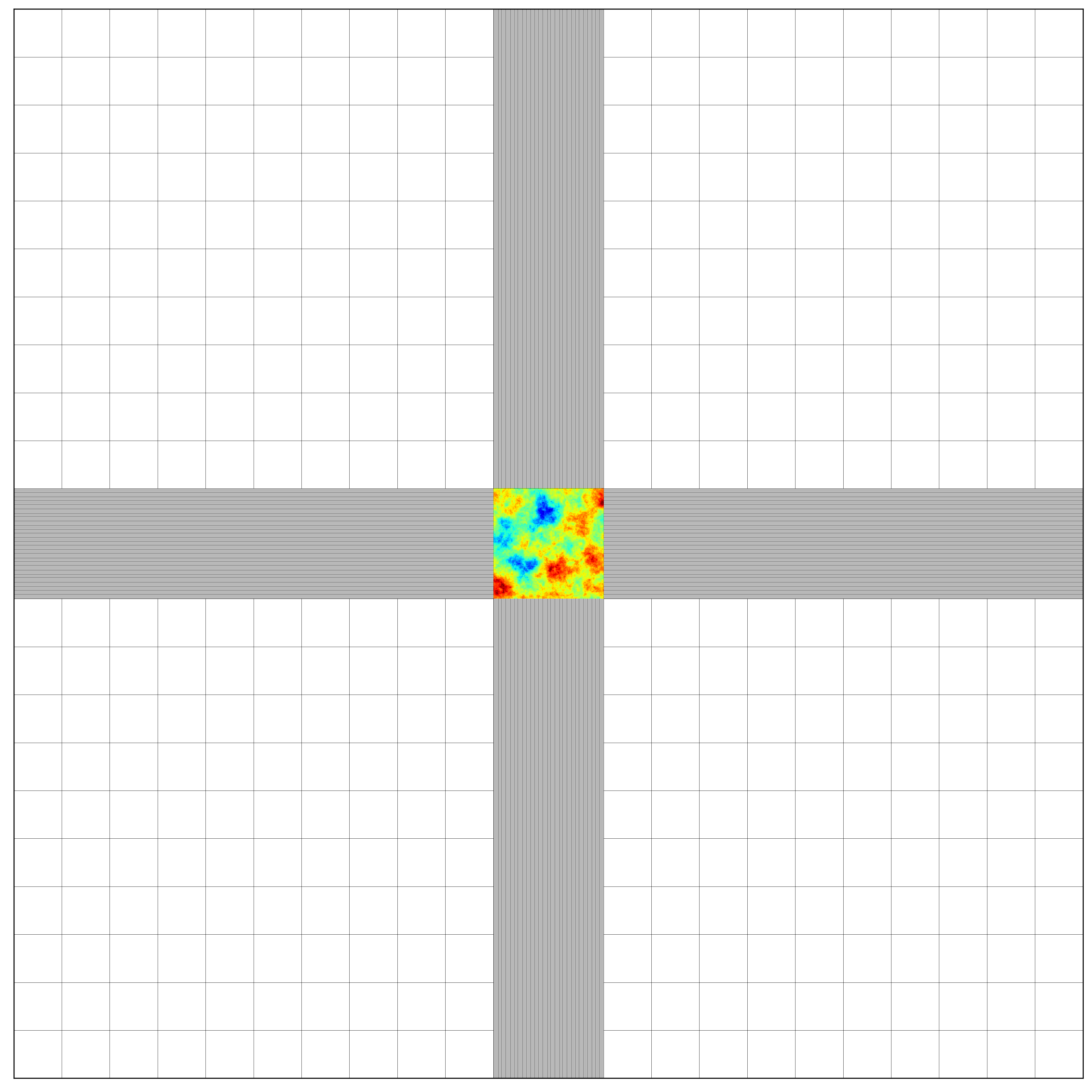
(a) Full domain including central storage aquifer and large surrounding region

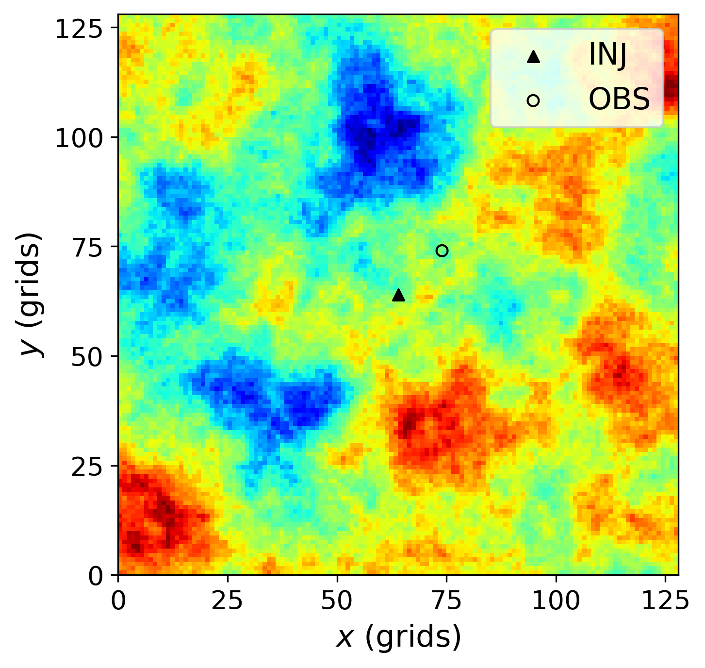
(b) Storage aquifer with injector and monitoring (observation) well

Figure 1: Model and wells used in all simulations.

2.2 Metaparameters and geomodels

In this work, geomodels characterized by a set of scenario parameters, referred to as metaparameters, are considered. For any set of metaparameters, an infinite number of geomodel realizations can be generated, each with a different property distribution. These metaparameters, denoted by $\mathbf{h}$, are represented as

$$\mathbf{h}=\left[\mu_{\log k},\sigma_{\log k},\log_{10}a_{r},d,e\right],$$ (1)

where $\mu_{\log k}$ and $\sigma_{\log k}$ denote the mean and standard deviation of the log-permeability field, $a_{r}$ is the anisotropy ratio between the vertical and horizontal permeability, i.e., $a_{r}=k_{v}/k_{h}$, where $k_{v}=k_{z}$ is the vertical permeability and $k_{h}=k_{x}=k_{y}$ is the horizontal permeability, and $d$ and $e$ are parameters that relate porosity and log-permeability. We denote the storage aquifer porosity and permeability fields as $\boldsymbol{\phi}_{s}\in\mathbb{R}^{n_{s}\times 1}$ and $\mathbf{k}_{s}\in\mathbb{R}^{n_{s}\times 1}$, where $n_{s}$ is the total number of grid blocks in the storage aquifer. The relationship between porosity and permeability is given by

$$(\phi_{s})_{i}=d\cdot(\log k_{s})_{i}+e,\quad i=1,\ldots,n_{s},$$ (2)

where $(\phi_{s})_{i}$ and $(\log k_{s})_{i}$ are porosity and log-permeability for grid block $i$.

The metaparameters associated with the storage aquifer are taken to be uncertain. These parameters and their (prior) ranges are shown in Table 1. The MCMC procedure applied in this work will act to reduce these uncertainty ranges.

Table 1: Metaparameters and ranges

Metaparameter Range Mean of log-permeability, $\mu_{\log k}$ $U$[2, 6] Standard deviation of log-permeability, $\sigma_{\log k}$ $U$[1.0, 2.5] Log of permeability anisotropy ratio, $\log_{10}a_{r}$ $U$[-2, 0] Parameter $d$ (in Eq. 2) $U$[0.02, 0.05] Parameter $e$ (in Eq. 2) $U$[0.05, 0.12]

Our procedure for constructing geological realizations of the storage aquifer follows the approach of Han et al. (2024). The first step involves the application of principal component analysis (PCA) to a set of prior realizations of standard Gaussian fields of prescribed correlation structure. These realizations are generated using the Stanford Geostatistical Modeling Software package, SGeMS (Remy et al., 2009). A spherical variogram, with correlation lengths in $x$, $y$, and $z$ of $l_{x}=l_{y}=280$ m and $l_{z}=7$ m, is specified for all realizations. The use of PCA allows us to avoid running SGeMS during online computations. This accelerates the overall workflow since the overhead associated with SGeMS can be significant.

The PCA representation is constructed through application of singular value decomposition (SVD) to the matrix containing, as its columns, the centered realizations generated using SGeMS. With this representation, new (random) realizations that honor the prescribed correlation structure can be generated using

$$\mathbf{y}_{pca}=\Phi\boldsymbol{\xi}+\overline{\mathbf{y}}.$$ (3)

Here $\mathbf{y}_{pca}\in\mathbb{R}^{n_{s}\times 1}$ is a new (PCA-based) realization, $\Phi\in\mathbb{R}^{n_{s}\times n_{d}}$ denotes the basis matrix obtained from SVD, truncated based on the $n_{d}$ largest singular values and corresponding left singular vectors, $\boldsymbol{\xi}\in\mathbb{R}^{n_{d}\times 1}$ is a stochastic vector with each component sampled from $\mathcal{N}(0,1)$, and $\overline{\mathbf{y}}\in\mathbb{R}^{n_{s}\times 1}$ is the mean of the SGeMS realizations. With this representation, the high-dimensional Gaussian field is parameterized with a low-dimensional latent vector $\boldsymbol{\xi}$.

Given a set of metaparameters $\mathbf{h}$ and the PCA representation $\mathbf{y}_{pca}(\boldsymbol{\xi})$, the full storage aquifer geomodel, which we denote as $\mathbf{m}=\mathbf{m}(\mathbf{h},\boldsymbol{\xi})$, is constructed as follows. Permeability (in $x$ and $y$) in each grid block is given by

$$(\log k_{s})_{i}=\sigma_{\log k}\cdot(y_{pca})_{i}+\mu_{\log k},\quad i=1,\ldots,n_{s},$$ (4)

where $(y_{pca})_{i}$ is the component of $\mathbf{y}_{pca}$ corresponding to block $i$. The vertical permeability is given by $(k_{z})_{i}=a_{r}\cdot(k_{s})_{i}$, and porosity is computed from Eq. 2. We reiterate that, in our history matching, both $\mathbf{h}$ and $\boldsymbol{\xi}$ are considered to be uncertain.

Cutoffs are applied to the PCA-generated permeability and porosity to avoid extreme (nonphysical) values. For permeability, the maximum and minimum values are $10^{4}$ mD and $10^{-4}$ mD, and for porosity they are 0.35 and 0.05.

2.3 Generation of interpreted 4D seismic data

In practice, seismic interpretations are obtained by solving geophysical inverse problems. This involves the use of measured seismic data of various types, and the seismic inversion provides parameters such as seismic velocities, acoustic impedance, density, etc. (Oliver et al., 2021). In the case of 4D seismic monitoring, data are collected at a sequence of times, and the data are inverted to obtain estimates of pressure and saturation throughout the domain.

In our framework, rather than use (and invert) ‘raw’ 4D seismic data, we assume that we are provided with estimates of gas (supercritical CO₂) saturation. These interpreted estimates are considered to be at the level of resolution achieved by 4D seismic data. This is, we believe, a reasonable approach, since the time-lapse seismic data are often treated and interpreted in a workflow that is distinct from the flow-based data assimilation process. An analogous approach, in the context of history matching for oil reservoir simulation, was applied by Bukshtynov et al. (2015).

We now describe how interpreted 4D seismic data are generated from flow simulation results for a highly resolved geomodel. The simulation provides CO₂ saturation fields (for the storage aquifer) on a grid of dimensions 128 $\times$ 128 $\times$ 35, with cells of size 7 m $\times$ 7 m $\times$ 2 m. The resolution of interpreted 4D seismic data depends on the seismic wavelength and other parameters, but a typical resolution level is about 20 m horizontally and 10 m vertically (Souza et al., 2019). A resolution of 21 m $\times$ 21 m $\times$ 10 m corresponds to a 3 $\times$ 3 $\times$ 5 filtering of our fine-scale saturation fields. We now describe the details of this filtering.

A two-step filtering, illustrated in Figure 2, is applied to generate the interpreted seismic data. The first step acts to smooth the original simulation results, and the second step resamples the smoothed results onto a coarser grid. This two-step approach reduces the ‘blockiness’ that could occur if a direct (one-step) averaging was used. In the first step, the filter is applied with a stride of 1, so the dimensions of the filtered results are 126 $\times$ 126 $\times$ 31. In the second step, we use a stride of 3 in the horizontal directions and 5 in the vertical direction, yielding a result of dimensions 42 $\times$ 42 $\times$ 7. Interpreted seismic data at these dimensions (42 $\times$ 42 $\times$ 7) will be used in our workflow.

The method described above is straightforward and provides us with a means to generate interpreted seismic saturation data, at the appropriate scale, from a high-fidelity geomodel. It is important to note that our treatment for generating interpreted seismic saturation data can be readily modified to include different smoothing, filtering or averaging procedures, or to account for saturation thresholding, etc. Such modifications might be appropriate in some settings to provide improved mappings from high-fidelity saturation fields to interpreted seismic fields. Note also that noise, which is intended to represent data and model errors, will be incorporated into the interpreted seismic data used for history matching. Our specific treatment for this is described in Section 6.1.

Figure 2: Schematic diagram showing the workflow for generating interpreted seismic data from high-fidelity simulation results. Images on the left are $x$-$z$ cross sections from the full 3D model, on the right are $y$-$z$ cross sections from the 3D model.

3 Deep learning surrogate models

The MCMC-based history matching procedure applied in this study requires a large number (e.g., $O(10^{4}-10^{5})$) of flow simulation results for evaluation of the likelihood function. Because MCMC is essentially a sequential algorithm, the elapsed time required for history matching would be prohibitive if high-fidelity simulations were performed for all function evaluations. Deep learning surrogate models have been shown to be very effective for this type of application. As discussed in the Introduction, many such models have been developed for subsurface flow problems.

In this study, we require predictions for the global saturation field at the time-lapse seismic-resolution scale, and for monitoring-well data at high vertical resolution but at one (or potentially a few) spatial locations. These data types are very different, and it would be inefficient to construct and train a single surrogate model to predict both sets of data. Therefore, we develop separate, fit-for-purpose surrogate models for each data type. With this approach, we can use simpler networks that do not require time-consuming training or need an excessive amount of training data. We now describe these models in turn.

3.1 Surrogate model for seismic data

The seismic surrogate model accepts the detailed geomodel as input. It then provides interpreted saturation, at the seismic resolution scale and at a specified number of time steps, as output. This prediction process, denoted $f_{\text{seis}}$, can be expressed as follows:

$$\hat{\textbf{S}}_{\text{seis}}=f_{\text{seis}}(\mathbf{k},\boldsymbol{\phi},a_{r};\theta_{seis}).$$ (5)

Here $\hat{\textbf{S}}_{\text{seis}}\in\mathbb{R}^{n_{x}^{seis}\times n_{y}^{seis}\times n_{z}^{seis}\times n_{t}^{s}}$ denotes the interpreted seismic prediction, with $n_{x}^{seis}$, $n_{y}^{seis}$, and $n_{z}^{seis}$ the dimension of the interpreted saturation field and $n_{t}^{s}$ the number of (4D seismic) time steps, and $\mathbf{k}\in\mathbb{R}^{n_{x}\times n_{y}\times n_{z}}$ and $\boldsymbol{\phi}\in\mathbb{R}^{n_{x}\times n_{y}\times n_{z}}$ denote the high-resolution permeability and porosity fields ($n_{x}$, $n_{y}$, and $n_{z}$ are the number of grid blocks in the storage aquifer in the $x$, $y$, and $z$ directions). In this work $a_{r}\in\mathbb{R}$ is taken to be constant over the spatial domain for a particular geomodel, so a 3D field with constant elements is used for this input. The quantity $\theta_{seis}$ indicates the trainable network parameters.

The U-Net architecture, shown in Figure 3, is used for the interpreted-seismic surrogate model. This network has three input channels, which define the high-resolution geomodel. There are multiple output channels, with each channel representing interpreted saturation at a single time step. We reiterate that the input and output properties are at different scales. The detailed architecture of the U-Net surrogate model is provided in Table 2. Specifics on the downsampling and upsampling layers in the encoder and decoder portions of the U-Net are given in Tables 3 and 4.

This U-Net architecture shares similarities with the networks used by Ronneberger et al. (2015) and Çiçek et al. (2016). Both of these are end-to-end learning models that were utilized for image segmentation. The task here – approximating the relationship between geomodel properties and interpreted seismic saturation fields – is also end-to-end, which makes this architecture appropriate for the seismic surrogate model. The skip-connections between the encoder and decoder are typical U-Net characteristics. These enable the network to effectively capture spatial features extracted at both high and low levels during the downsampling process.

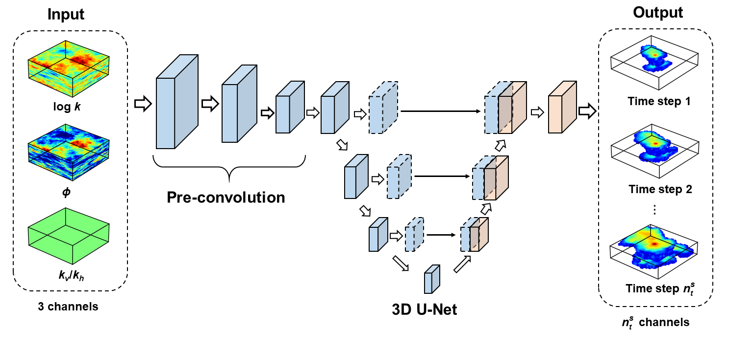
Figure 3: Schematic of U-Net surrogate model used to predict interpreted seismic saturation data.

Table 2: Detailed architecture of the U-Net surrogate model for (interpreted seismic) saturation prediction

Module Layers Output size Preconvolution Input (3$\times$128$\times$128$\times$35) Conv, 64 filters of size 3$\times$3$\times$5, stride (1, 1, 1), padding (0, 0, 1) 64$\times$126$\times$126$\times$33 Activation (Swish) 64$\times$126$\times$126$\times$33 Conv, 32 filters of size 3$\times$3$\times$5, stride (3, 3, 5), padding (0, 0, 1) 32$\times$42$\times$42$\times$7 Activation (Swish) 32$\times$42$\times$42$\times$7 Encoder Downsample, 32 filters of size 3$\times$3$\times$3, stride (1, 1, 1), padding (0, 0, 1) 32$\times$40$\times$40$\times$7 Downsample, 64 filters of size 4$\times$4$\times$3, stride (2, 2, 1), padding (0, 0, 1) 64$\times$19$\times$19$\times$7 Downsample, 128 filters of size 3$\times$3$\times$3, stride (2, 2, 1), padding (0, 0, 0) 128$\times$9$\times$9$\times$5 Downsample, 256 filters of size 3$\times$3$\times$3, stride (2, 2, 1), padding (0, 0, 0) 256$\times$4$\times$4$\times$3 Decoder Upsample, 256 filters of size 3$\times$3$\times$3, stride (2, 2, 1), padding (0, 0, 0) 256$\times$9$\times$9$\times$5 Upsample, 128 filters of size 3$\times$3$\times$3, stride (2, 2, 1), padding (0, 0, 0) 128$\times$19$\times$19$\times$7 Upsample, 64 filters of size 4$\times$4$\times$3, stride (2, 2, 1), padding (0, 0, 1) 64$\times$40$\times$40$\times$7 Upsample, 32 filters of size 3$\times$3$\times$3, stride (1, 1, 1), padding (0, 0, 1) 32$\times$42$\times$42$\times$7 Output Conv, 32 filters of size 3$\times$3$\times$3, stride (1, 1, 1), padding (1, 1, 1) 32$\times$42$\times$42$\times$7 Activation (Swish) 32$\times$42$\times$42$\times$7 Conv, 6 filters of size 3$\times$3$\times$3, stride (1, 1, 1), padding (1, 1, 1) 6$\times$42$\times$42$\times$7

Table 3: Architecture of downsampling layers in the U-Net

Layers Input Conv, $n_{\text{channel}}$ (defined in Table 2 or 5) filters with size 3, stride 1, padding 1 Activation (ReLU) Conv, $n_{\text{channel}}$ (defined in Table 2 or 5) filters with size, stride, and padding defined in Table 2 or 5 Activation (ReLU)

Table 4: Architecture of upsampling layers in the U-Net

Layers Input ConvTranspose, $n_{\text{channel}}$ (defined in Table 2 or 5)$\times 2$ filters with size 3, stride 1, padding 1 Activation (ReLU) ConvTranspose, $n_{\text{channel}}$ (defined in Table 2 or 5) filters with size, stride, and padding defined in Table 2 or 5 Activation (ReLU)

To train the surrogate model, the mismatch between the predicted and reference (interpreted seismic) saturation fields is minimized over a large set of geomodel realizations (the training set). These realizations are constructed by sampling the metaparameters from the ranges given in Table 1 and the components of $\boldsymbol{\xi}$ from ${\mathcal{N}}(0,1)$, as described earlier. Flow simulation is performed using GEOS (more details on the setup will be provided in Section 5.1). The filtered saturation fields provide the reference results. The loss function is given by

$$L_{\text{seis}}(\theta_{seis})=\frac{1}{n_{x}^{seis}n_{y}^{seis}n_{z}^{seis}n_{t}^{s}}\frac{1}{N}\sum_{i=1}^{N}\|\hat{{\mathbf{S}}}_{\text{seis},i}-{\mathbf{S}}_{\text{seis},i}\|_{2}^{2},$$ (6)

where $N$ denotes the number of geomodel realizations used for training, $\textbf{S}_{\text{seis},i}$ denotes the reference interpreted seismic saturation field for training sample $i$, and $\hat{{\mathbf{S}}}_{\text{seis},i}$ indicates the surrogate model prediction for sample $i$. The model is trained by adjusting the network parameters $\theta_{seis}$ to minimize $L_{\text{seis}}$. This is accomplished with the Adam optimization algorithm (Kingma and Ba, 2014) on a Nvidia A100 GPU. The initial learning rate is set to be $10^{-4}$, which is updated by multiplying by a factor of 0.2 when the performance does not improve for 10 epochs. The minimum learning rate is set to be $10^{-7}$.

3.2 Surrogate model for monitoring-well data

We now describe the surrogate model used to predict the CO₂ saturation profile (in $z$) at the monitoring well at a series of time steps. The surrogate model prediction of the monitoring data, $f_{\text{mon}}$, can be expressed as

$$\hat{\textbf{S}}_{\text{mon}}=f_{\text{mon}}(\mathbf{k}_{\text{local}},\boldsymbol{\phi}_{\text{local}},a_{r};\theta_{mon}).$$ (7)

Here $\hat{\textbf{S}}_{\text{mon}}\in\mathbb{R}^{n_{z}\times n_{t}^{m}}$ denotes the predicted saturation at the monitoring well, at all $n_{z}$ layers at $n_{t}^{m}$ time steps, $\mathbf{k}_{\text{local}}\in\mathbb{R}^{n_{x}^{l}\times n_{y}^{l}\times n_{z}}$ and $\boldsymbol{\phi}_{\text{local}}\in\mathbb{R}^{n_{x}^{l}\times n_{y}^{l}\times n_{z}}$ denote the permeability and porosity in a set of cells in a local $x$-$y$ region (at all values of $z$) encompassing the injection well and monitoring well, with $n_{x}^{l}$ and $n_{y}^{l}$ the number of local cells in the $x$ and $y$ directions. The trainable parameters for this network are denoted $\theta_{mon}$.

We use a 1D U-Net architecture, shown in Figure 4, for the monitoring data surrogate model. The surrogate model outputs a series of 1D vectors – the elements of these vectors are the predicted saturation values for all $n_{z}$ cells at the monitoring location at a particular time. There are multiple output channels, with each channel providing the saturation profile at a single time step. The saturation vectors at different time steps can then be combined to form a 2D map of dimensions $n_{z}\times n_{t}^{m}$, as shown in Figure 4. This map displays the evolution of the vertical saturation profile through time.

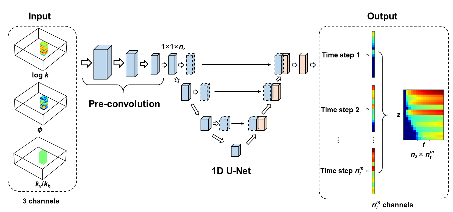
Figure 4: Architecture of 1D U-Net surrogate for monitoring data.

The monitoring well saturation data are most impacted by storage aquifer properties in the vicinity of the injection and monitoring wells. As noted in Section 2.1, the injection well is located at areal coordinates $(i,j)=(65,65)$, and the monitoring well is located at $(i,j)=(75,75)$. The local geomodel information provided in the network inputs $\mathbf{k}_{\text{local}}$ and $\boldsymbol{\phi}_{\text{local}}$ is over the region $i=63,\ldots,81$, $j=63,\ldots,81$, $k=1,\ldots,35$ (here $k$ is the index in the $z$ direction). Thus the local region includes all layers within a domain that incorporates (with some padding) the injection well and monitoring well. These ranges for the local region correspond to $n_{x}^{l}=n_{y}^{l}=19$.

We apply the 1D U-Net architecture for this surrogate model because the data we seek to represent are themselves a series of 1D vectors. Specifically, the 1D convolutional layers can capture features along the vectors, which correspond to the saturation as a function of depth. Similar network architectures were also used in previous studies predicting 1D signals (Hou et al., 2021; Chen et al., 2023). The detailed architecture of the 1D U-Net surrogate model is provided in Table 5. Specifications for the residual blocks utilized in the 1D U-Net are given in Table 6.

The loss function to be minimized in the training process for the 1D U-Net surrogate is given by

$$L_{\text{mon}}(\theta_{mon})=\frac{1}{n_{z}n_{t}^{m}}\frac{1}{N}\sum_{i=1}^{N}\left|\hat{\textbf{S}}_{\text{mon},i}-\textbf{S}_{\text{mon},i}\right|,$$ (8)

where $\textbf{S}_{\text{mon},i}\in\mathbb{R}^{n_{z}\times n_{t}^{m}}$ denotes the reference result for the saturation profile at the monitoring well location at $n_{t}^{m}$ time steps for training sample $i$, and $\hat{\textbf{S}}_{\text{mon},i}$ is the corresponding surrogate model prediction. The RAdam algorithm is adopted to train the network (Liu et al., 2019). The initial learning rate is 0.001, which decays with a factor of 0.2 when the performance does not improve for 5 epochs. The minimum learning rate is again $10^{-7}$. The training process is implemented on a Nvidia A100 GPU.

The two trained surrogate models can now be used for history matching CO₂ storage operations where both 4D seismic and monitoring well data are available. Our framework is flexible, and could be easily extended to handle, e.g., pressure data measured at the monitoring well (though this was not attempted here). Either surrogate model could also be modified or enhanced as necessary to treat more complicated geomodels. We now describe the MCMC history matching procedure.

Table 5: Detailed architecture of the 1D U-Net surrogate model for prediction of monitoring well data

Module Layers Output size Preconvolution Input (3$\times$19$\times$19$\times$35) Conv, 16 filters of size 3$\times$3$\times$3, stride (1, 1, 1), padding (0, 0, 1) 16$\times$17$\times$17$\times$35 Activation (Swish) 16$\times$17$\times$17$\times$35 Conv, 32 filters of size 3$\times$3$\times$3, stride (2, 2, 1), padding (1, 1, 1) 32$\times$9$\times$9$\times$35 Activation (Swish) 32$\times$9$\times$9$\times$35 Conv, 64 filters of size 5$\times$5$\times$3, stride (2, 2, 1), padding (0, 0, 1) 64$\times$3$\times$3$\times$35 Activation (Swish) 64$\times$3$\times$3$\times$35 Conv, 128 filters of size 3$\times$3$\times$3, stride (1, 1, 1), padding (0, 0, 1) 128$\times$1$\times$1$\times$35 Activation (Swish) 128$\times$1$\times$1$\times$35 Encoder Downsample, 64 filters of size 3, stride 1, padding 0 64$\times$33 Downsample, 128 filters of size 3, stride 1, padding 0 128$\times$31 Downsample, 256 filters of size 3, stride 2, padding 0 256$\times$15 Downsample, 512 filters of size 3, stride 2, padding 0 512$\times$7 Residual Residual block, 512 filters of size 3, stride 1, padding 1 512$\times$7 Residual block, 512 filters of size 3, stride 1, padding 1 512$\times$7 Residual block, 512 filters of size 3, stride 1, padding 1 512$\times$7 Residual block, 512 filters of size 3, stride 1, padding 1 512$\times$7 Decoder Upsample, 512 filters of size 3, stride 2, padding 0 512$\times$15 Upsample, 256 filters of size 3, stride 2, padding 0 256$\times$31 Upsample, 128 filters of size 3, stride 1, padding 0 128$\times$33 Upsample, 64 filters of size 3, stride 1, padding 0 64$\times$35 Output part Conv, 64 filters of size 3, stride 1, padding 1 64$\times$35 Activation (Swish) 64$\times$35 Conv, 16 filters of size 3, stride 1, padding 1 16$\times$35

Table 6: Architecture of residual block in the 1D U-Net

Layers Input Conv, $n_{\text{channel}}$ (defined in Table 5) filters with size 3, stride 1, padding 1 Activation (ReLU) Conv, $n_{\text{channel}}$ (defined in Table 5) filters with size 3, stride 1, padding 1 Addition (with input) Activation (ReLU)

4 Hierarchical MCMC method and overall workflow

Our data assimilation problem is similar to that considered by Han et al. (2024) in that both metaparameters and associated geomodel realizations must be determined (the previous study did not consider 4D seismic data so the setup is otherwise quite different). Thus, we apply the hierarchical Markov Chain Monte Carlo (MCMC) method used in that work. MCMC is a widely used history matching technique in which geomodels are sampled iteratively and the likelihood, which involves the data mismatch, is evaluated for each sample. After a large number of iterations, the accepted samples can approximate the posterior distributions. In hierarchical MCMC, two levels of sampling are applied – one for the metaparameters $\mathbf{h}$, and one for the PCA latent variables, $\boldsymbol{\xi}$. Upon convergence (termination), we have an estimate of the posterior probability density function (PDF) $p(\boldsymbol{\xi},\mathbf{h}\mid\mathbf{d}_{\text{obs}})$, where $\mathbf{d}_{\text{obs}}$ denotes the observed data. Because MCMC methods require a large number of sequential function evaluations (e.g., $O(10^{4}-10^{5})$, the use of surrogate models is essential in cases with expensive function evaluations, such as ours.

We now describe the hierarchical procedure. Our description here follows Han et al. (2024), and that work should be consulted for details. In the first level, the PCA latent variables are sampled. The initial sample is obtained by sampling each PCA variable from ${\mathcal{N}}(0,1)$. Subsequently, a stochastic perturbation is applied to the previous samples to obtain the new sample. Specifically, the new sample $\boldsymbol{\xi}^{\prime}\in\mathbb{R}^{n_{d}\times 1}$ at iteration $k$ is given by

$$\boldsymbol{\xi}^{\prime}=(1-\beta^{2})\boldsymbol{\xi}^{k-1}+\beta\boldsymbol{\eta},$$ (9)

where $\boldsymbol{\xi}^{k-1}\in\mathbb{R}^{n_{d}\times 1}$ denotes the sample from the previous iteration, $\boldsymbol{\eta}\in\mathbb{R}^{n_{d}\times 1}$ denotes a stochastic vector with each element sampled from ${\mathcal{N}}(0,1)$, and $\beta\in\mathbb{R}$ is a user-defined hyperparameter that controls the size of the sample update and impacts the MCMC acceptance rate.

The acceptance or rejection of $\boldsymbol{\xi}^{\prime}$ depends on its likelihood. Here we use the Metropolis–Hastings (Hastings, 1970) criterion for this determination. With this approach, the acceptance probability for $\boldsymbol{\xi}^{\prime}$ is taken as

$$\alpha(\boldsymbol{\xi}^{k-1},\boldsymbol{\xi}^{\prime})=\min\left(1,\frac{p(\mathbf{d}_{\text{obs}}\mid\boldsymbol{\xi}^{\prime},\mathbf{h}^{k-1})}{p(\mathbf{d}_{\text{obs}}\mid\boldsymbol{\xi}^{k-1},\mathbf{h}^{k-1})}\right),$$ (10)

where $p(\mathbf{d}_{\text{obs}}\mid\boldsymbol{\xi}^{\prime},\mathbf{h}^{k-1})$ and $p(\mathbf{d}_{\text{obs}}\mid\boldsymbol{\xi}^{k-1},\mathbf{h}^{k-1})$ are the likelihood of the current sample $\boldsymbol{\xi}^{\prime}$ and the previous sample $\boldsymbol{\xi}^{k-1}$, both conditioned to metaparameter sample $\mathbf{h}^{k-1}$ from the previous iteration. The detailed likelihood function will be given in Section 6.1. A random variable $u_{\text{pca}}$ is then sampled from a uniform distribution $U[0,1]$. If $\alpha(\boldsymbol{\xi}^{k-1},\boldsymbol{\xi}^{\prime})>u_{\text{pca}}$, the new sample $\boldsymbol{\xi}^{\prime}$ is accepted, meaning $\boldsymbol{\xi}^{k}=\boldsymbol{\xi}^{\prime}$. Otherwise, the new sample is rejected, in which case $\boldsymbol{\xi}^{k}=\boldsymbol{\xi}^{k-1}$.

In the second level of hierarchical MCMC the metaparameters are sampled. The initial sample is obtained from the prior distribution. In later iterations, new metaparameters are proposed from a multivariate Gaussian distribution centered on the previously accepted sample. The standard deviations for these distributions are user-defined and problem specific (further details will be provided in Section 6). The acceptance probability for the newly sampled set of metaparameters $\mathbf{h}^{\prime}$ is analogous to that used for $\boldsymbol{\xi}^{\prime}$, i.e.,

$$\alpha(\mathbf{h}^{k-1},\mathbf{h}^{\prime})=\min\left(1,\frac{p(\mathbf{h}^{\prime})p(\mathbf{d}_{\text{obs}}\mid\boldsymbol{\xi}^{k},\mathbf{h}^{\prime})}{p(\mathbf{h}^{k-1})p(\mathbf{d}_{\text{obs}}\mid\boldsymbol{\xi}^{k},\mathbf{h}^{k-1})}\right).$$ (11)

Here $p(\mathbf{h}^{\prime})$ and $p(\mathbf{h}^{k-1})$ are prior probabilities of the proposed metaparameters $\mathbf{h}^{\prime}$ and previously accepted metaparameters $\mathbf{h}^{k-1}$, $p(\mathbf{d}_{\text{obs}}\mid\boldsymbol{\xi}^{k},\mathbf{h}^{\prime})$ and $p(\mathbf{d}_{\text{obs}}\mid\boldsymbol{\xi}^{k},\mathbf{h}^{k-1})$ denote the likelihood of $\mathbf{h}^{\prime}$ and $\mathbf{h}^{k-1}$, both conditioned to PCA variables in the current iteration ($\boldsymbol{\xi}^{k}$). As in the first step, we sample $u_{\text{meta}}$ from $U[0,1]$; if $\alpha(\mathbf{h}^{k-1},\mathbf{h}^{\prime})>u_{\text{meta}}$, the proposed metaparameters $\mathbf{h}^{\prime}$ are accepted, otherwise they are rejected.

The hierarchical MCMC procedure continues until a termination criterion is reached. Here, as in Nicolaidou et al. (2022) and Han et al. (2024), the procedure is terminated when the relative change in the posterior histogram for the metaparameters falls below a specified threshold. At that point, the accepted samples are taken to provide estimates of their corresponding posterior probability densities.

We now describe the overall workflow involving the use of our deep learning surrogate models in the hierarchical MCMC history matching framework. Figure 5 illustrates the two key components of the framework – surrogate model construction, accomplished in a preprocessing (offline) step, and (online) history matching. For surrogate model construction, the training data are generated by simulating a large number of geomodels. Each geomodel is generated by randomly sampling the metaparameters and PCA components. The data used for training the monitoring well surrogate are extracted directly from the high-fidelity simulation results, and the data for the seismic surrogate are obtained through use of the filtering procedure. In a real application, the actual monitoring well saturation and interpreted 4D seismic data would be used for history matching. In our examples these data are synthetic, i.e., generated by simulating a specific ‘true’ model and then adding noise. From the observed data (real or synthetic), the mismatch and likelihood are computed, with all function evaluations performed using the surrogate models. Following termination of the hierarchical MCMC procedure, a set of posterior geomodels and associated predictions are attained.

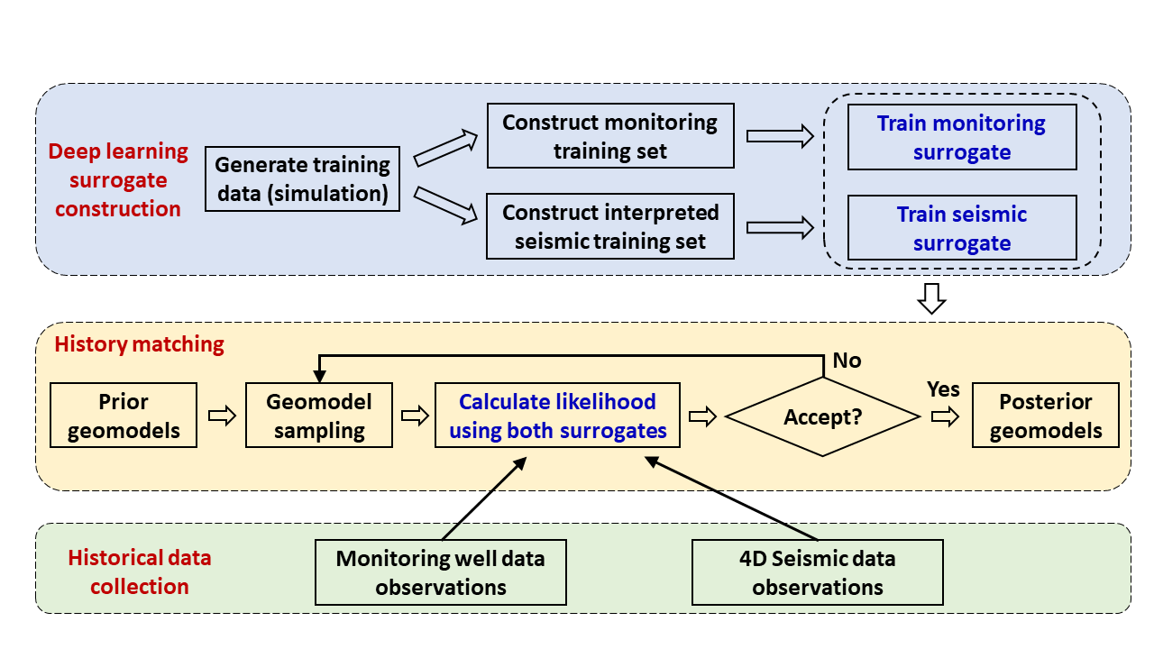
Figure 5: Deep-learning-based workflow for history matching using both monitoring well data and 4D seismic data.

5 Surrogate model evaluation

In this section, we describe the simulation setup and evaluate the performance of the surrogate models for a wide range of geomodel realizations.

5.1 Simulation setup

The model domain is illustrated in Figure 1, and aspects of the problem setup have been discussed in previous sections. We consider heterogeneous, multi-Gaussian log-permeability and porosity fields in the storage aquifer. The permeability and porosity in the surrounding region are set to constant values of 20 mD and 0.2.

The relative permeability and capillary pressure functions are generated from the Brooks-Corey model. The coefficients used here, shown in Table 7, derive from data reported for the Mt. Simon sandstone by Krevor et al. (2012). The capillary pressure curve is calculated using the Leverett J-function. Relative permeability curves for the CO₂–water system are presented in Figure 6(a), and the capillary pressure curve calculated for porosity of 0.2 and permeability of 20 md appear in Figure 6(b). The initial pressure (at a depth of 1955 m) is 20 MPa. Temperature at 1955 m depth is 50.3 ^∘C. The viscosity and density of CO₂ and brine/water are computed (as a function of pressure and temperature) in the simulator. All simulations are performed using GEOS, an open-source, multiphysics simulator designed for carbon storage modeling (Bui et al., 2021).

Table 7: Brooks-Corey model coefficients for relative permeability and capillary pressure functions

Coefficient Value Irreducible water saturation, $S_{wi}$ 0.22 Residual CO₂ saturation, $S_{gr}$ 0 Water exponent for Corey model, $n_{w}$ 9 CO₂ exponent for Corey model, $n_{g}$ 4 Relative permeability of CO₂ at $S_{wi}$, $k_{rg}(S_{wi})$ 0.95 Capillary pressure exponent, $\lambda$ 0.55

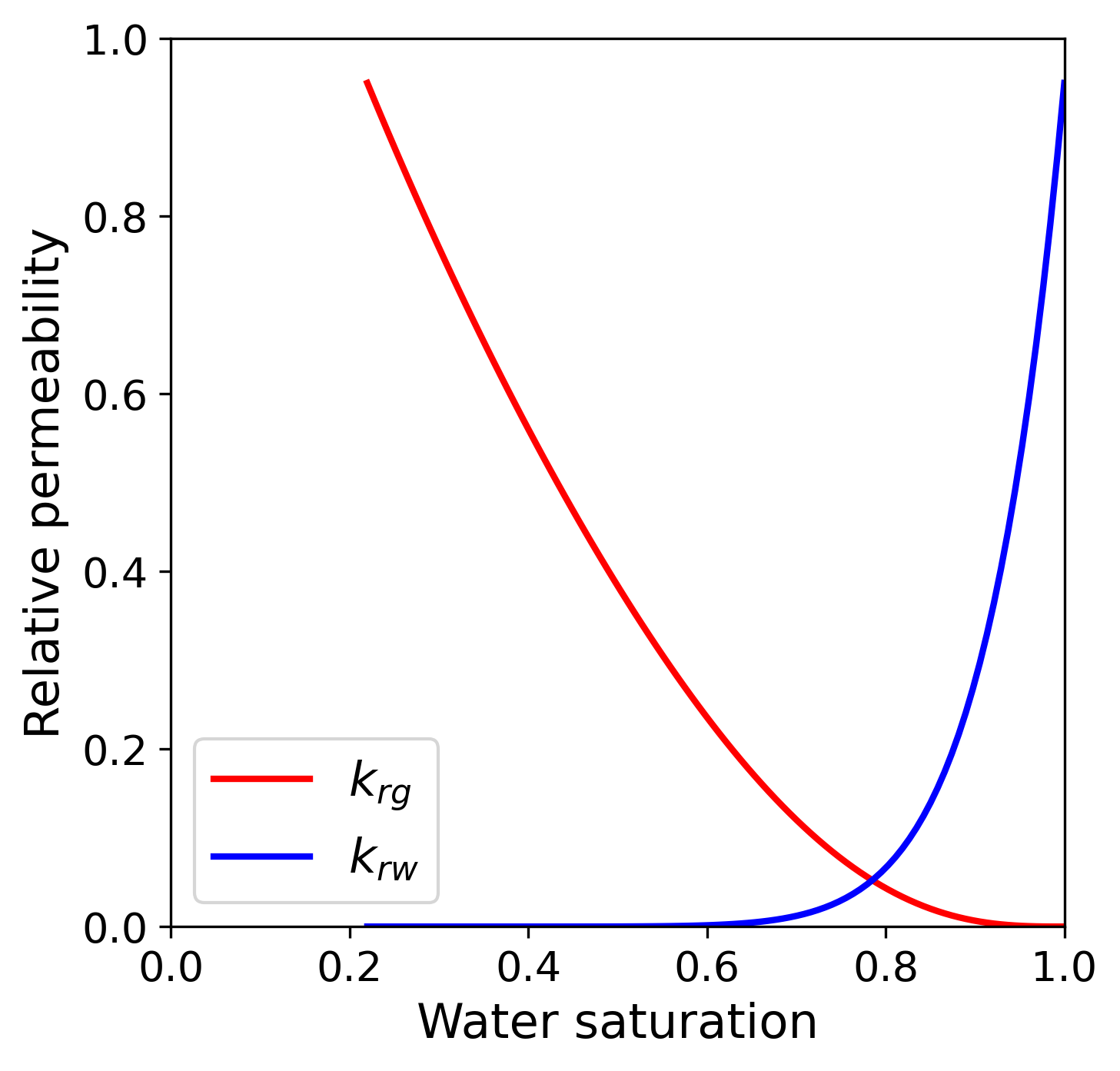
(a) Relative permeability

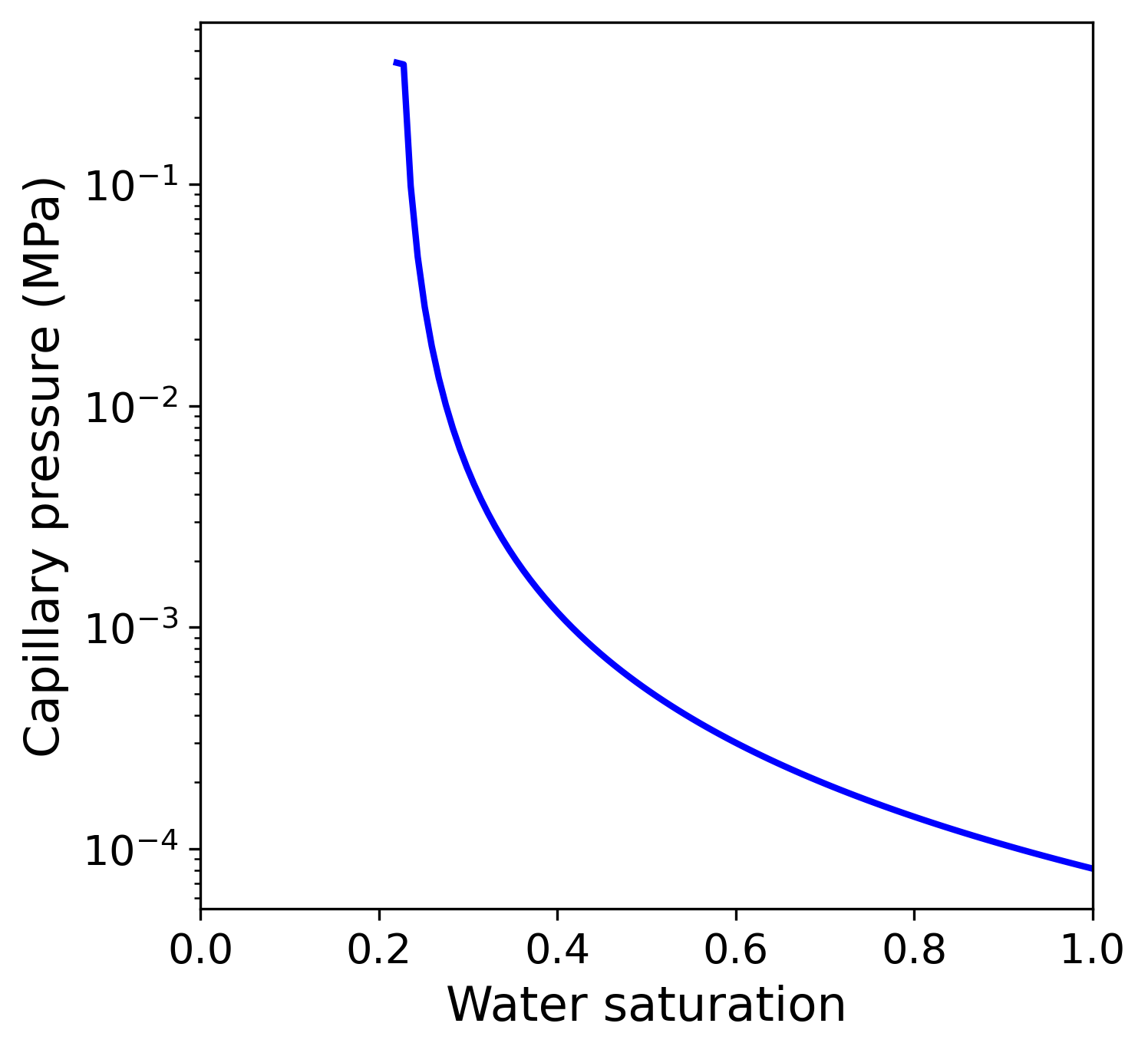
(b) Capillary pressure ($\phi=0.2$, $k=20$ md)

Figure 6: Relative permeability and capillary pressure curves for CO₂–brine system.

Since our interest is in early time behavior and history matching, the simulation time frame is restricted to 1 year, which is divided into 30 time steps. A total of 4000 geomodel realizations are generated and simulated for surrogate model training and evaluation. Of these models, 3500 comprise the training set and 500 comprise the test set. For each realization, the metaparameters are sampled from the ranges shown in Table 1, the PCA latent variables are sampled from ${\mathcal{N}}(0,1)$, and the procedure described in Section 2.2 is applied to construct the full geomodel. Following the flow simulation, the saturation fields are saved at a set of time steps. From these solutions the monitoring data are extracted and the interpreted seismic data are constructed.

5.2 Surrogate performance evaluation

Before assessing the accuracy of the surrogate models, we quantify the runtimes for high-fidelity simulation and surrogate evaluations. The GEOS runs require an average of about 38 minutes. This timing can vary from about 15 minutes to 200 minutes depending on time-step cutting, Newton iteration convergence, etc., which in turn depend on the geomodel. The surrogate models require less than 0.1 second to provide a function evaluation. It is this very high degree of speedup that enables the use of sophisticated history matching methods such as hierarchical MCMC. We now evaluate the performance of the two deep learning surrogate models.

5.2.1 4D seismic surrogate evaluation

The surrogate for 4D seismic data was described in Section 3.1. The model is trained to predict interpreted seismic data at six time steps, specifically time steps 5, 10, 15, 20, 25, and 30, which correspond to times of 2, 4, 6, 8, 10 and 12 months. The network architecture has six output channels – one for each of the six time steps. In the training process, the batch size of the training dataset is set to be 10, and the model is trained for 150 epochs with an initial learning rate of $10^{-4}$. The training process takes approximately 2 hours on a Nvidia A100 GPU.

We now show results for test-set models. Comparison between predicted seismic data and reference results (generated by simulating the test-case model and then filtering the saturation field), for three randomly selected realizations, are shown in Figure 7. These results are at a time of 1 year (last time step). It is evident that the predicted plume shapes (lower row) for the different realizations closely resemble the reference results (upper row). We also see that the saturation fields differ significantly between realizations.

Cross sections through the plumes for the three realizations, again at 1 year, are presented in Figure 8. These results are for the $x$-$z$ cross section through the injection well. Predictions from the surrogate model are in reasonable agreement with reference results, both for relatively uniform plumes (Figure 8(a)) and for irregular shaped plumes (Figure 8(b) and (c)).

(a) Realization 1 (sim)

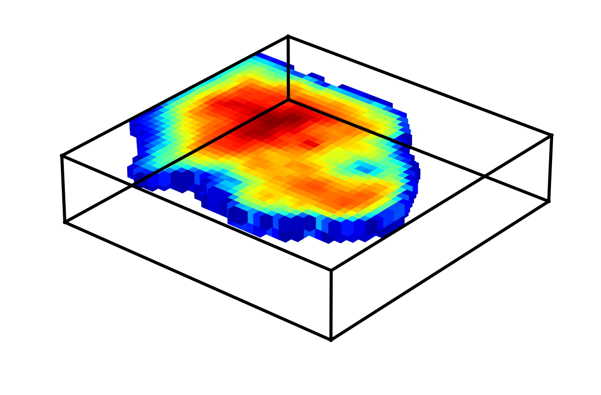
(b) Realization 2 (sim)

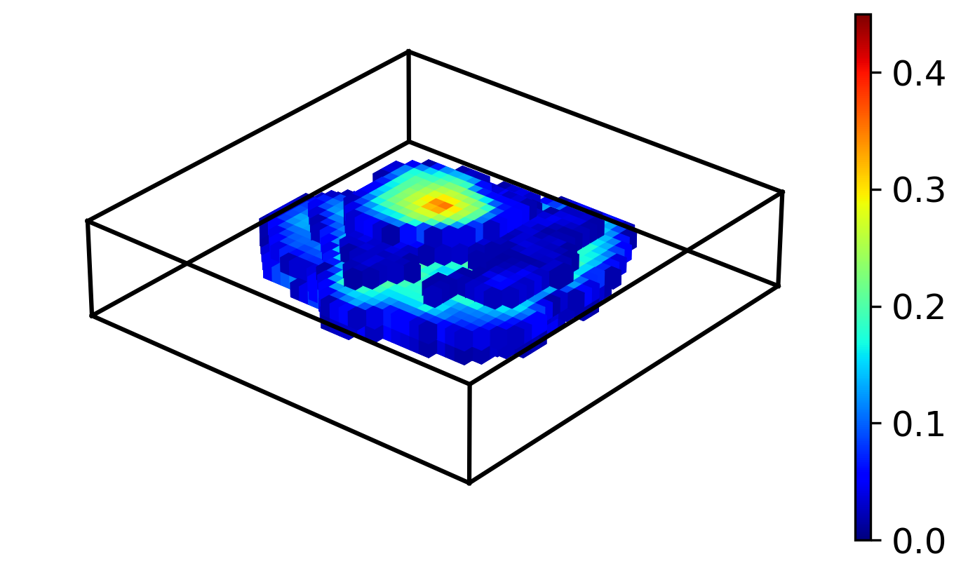
(c) Realization 3 (sim)

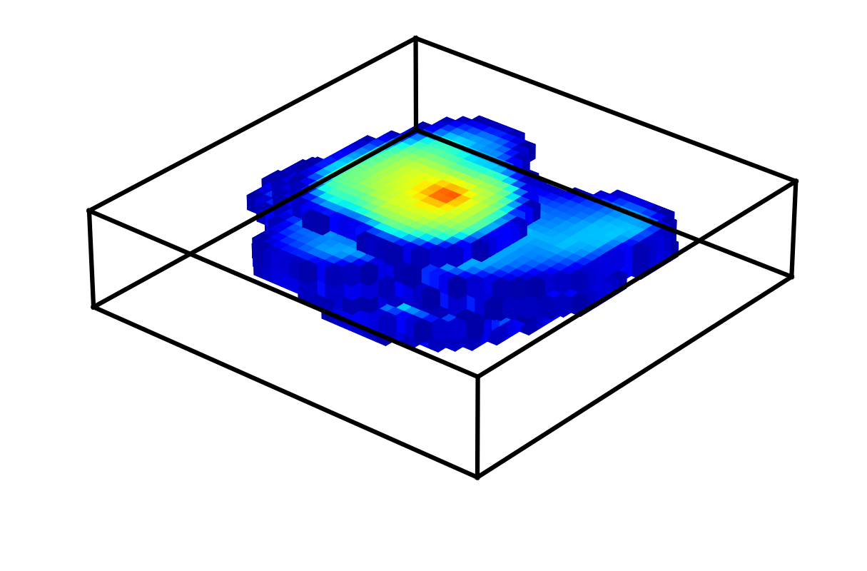
(d) Realization 1 (surr)

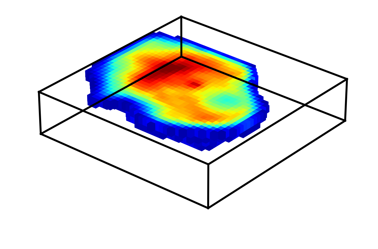
(e) Realization 2 (surr)

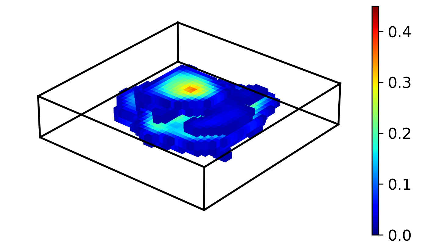
(f) Realization 3 (surr)

Figure 7: Comparison of surrogate model predictions (surr) and reference simulation results (sim) for interpreted seismic saturation fields for three realizations at 1 year.

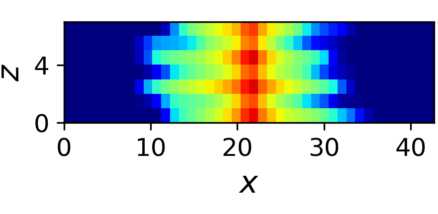
(a) Realization 1 (sim)

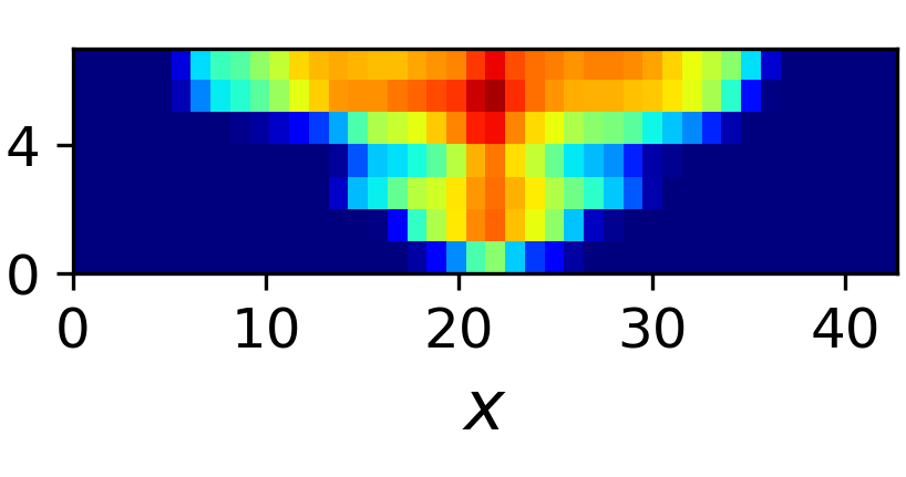
(b) Realization 2 (sim)

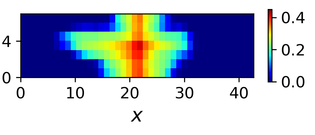
(c) Realization 3 (sim)

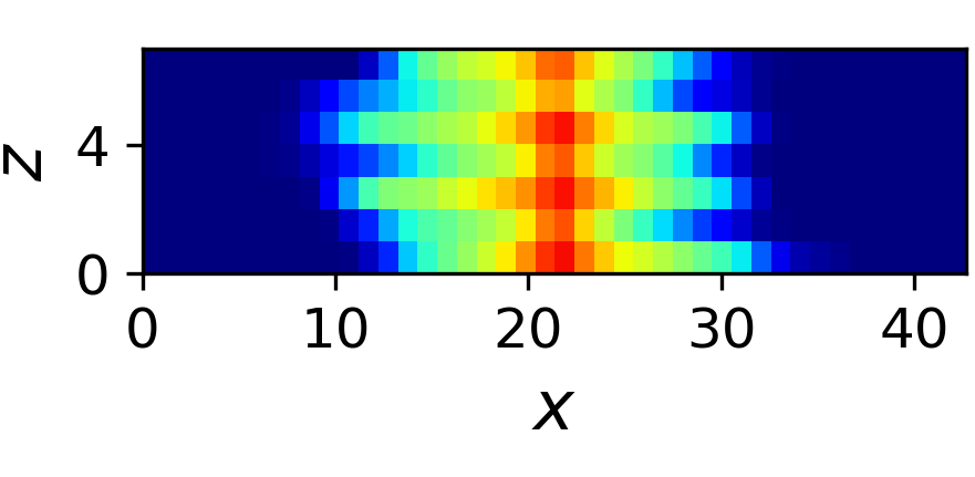
(d) Realization 1 (surr)

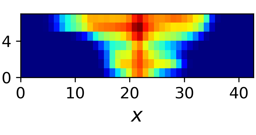
(e) Realization 2 (surr)

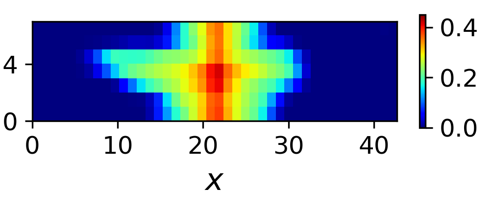
(f) Realization 3 (surr)

Figure 8: Comparison of surrogate model predictions (surr) and reference simulation results (sim) for interpreted seismic saturation fields, in $x$-$z$ cross sections through the injection well, for three realizations at 1 year.

We next present time-lapse results for a specific geomodel (Realization 2 in Figures 7 and 8). Interpreted saturation fields at five time steps are displayed in Figure 9. Although slight differences are evident at some steps, it is clear that the general time evolution is captured accurately by the surrogate model.

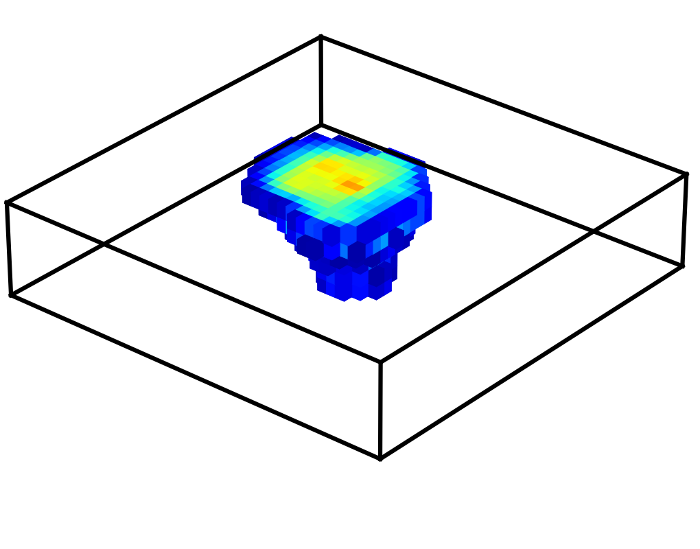
(a) 2 months (sim)

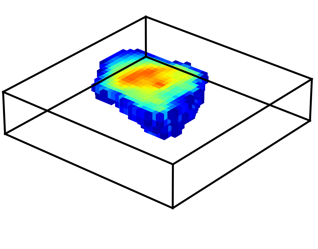
(b) 4 months (sim)

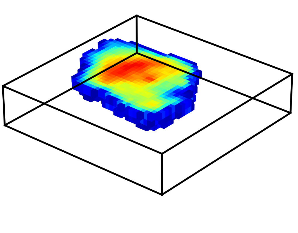
(c) 6 months (sim)

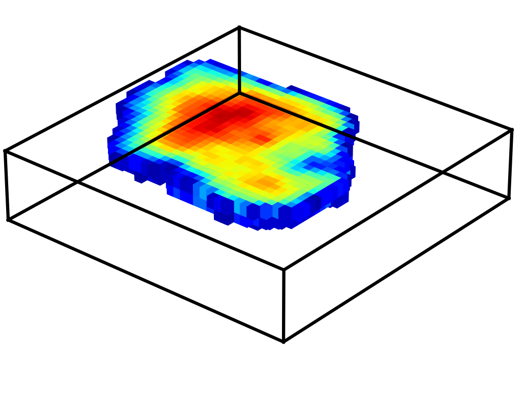
(d) 8 months (sim)

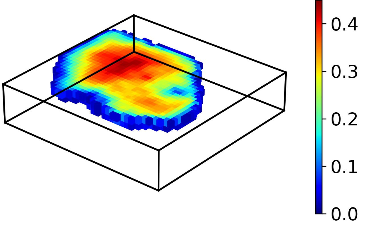
(e) 10 months (sim)

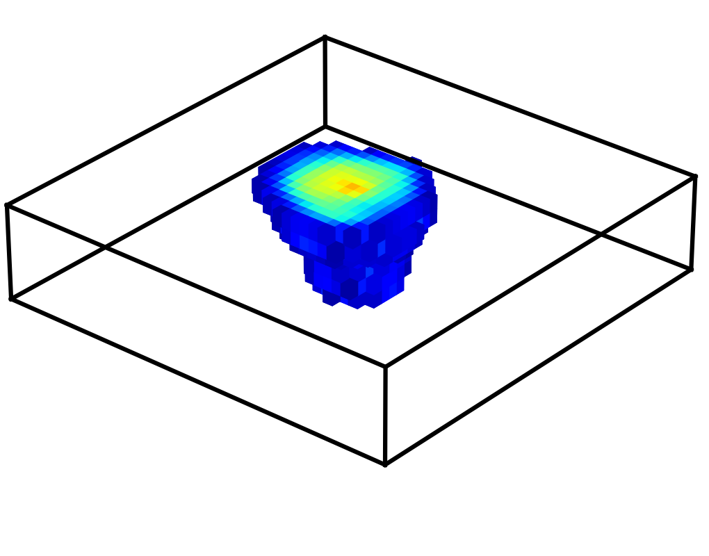
(f) 2 months (surr)

(g) 4 months (surr)

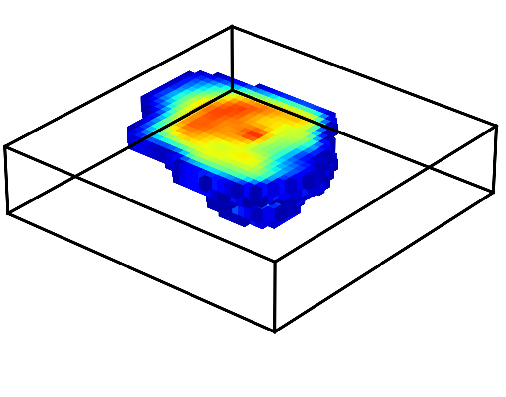
(h) 6 months (surr)

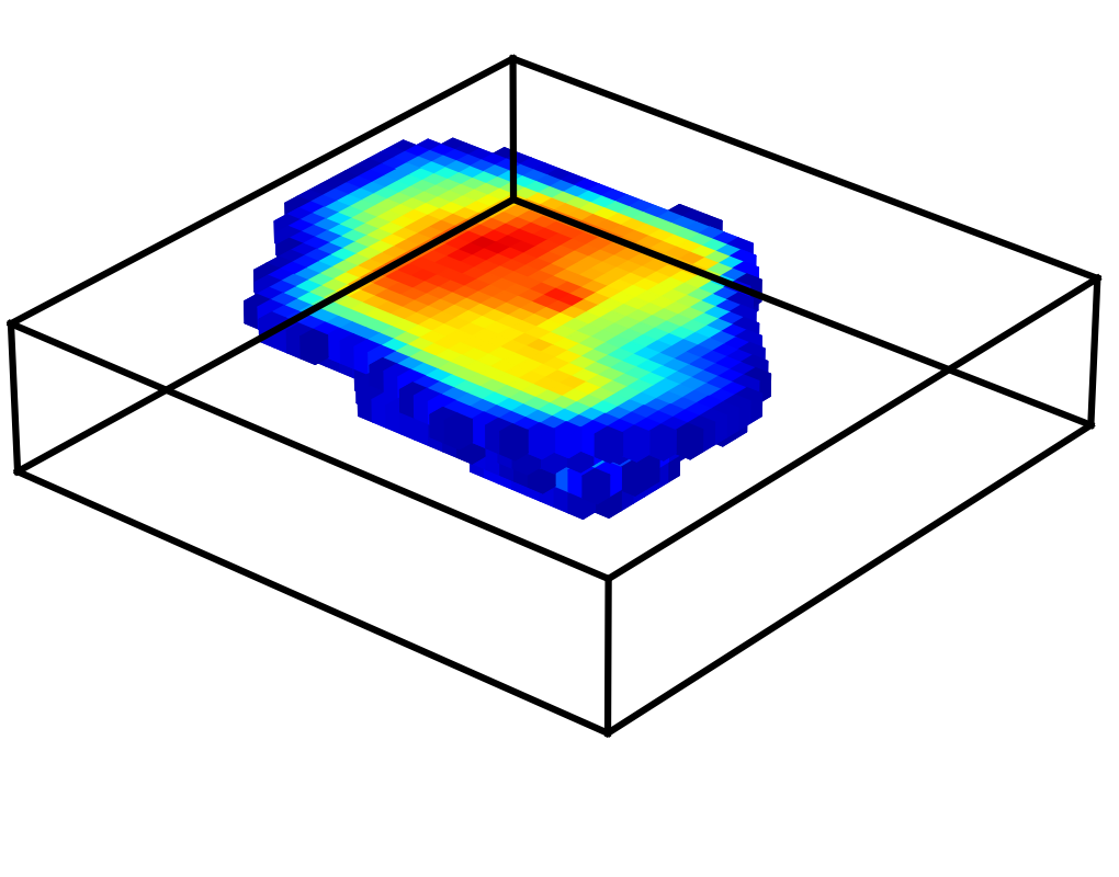
(i) 8 months (surr)

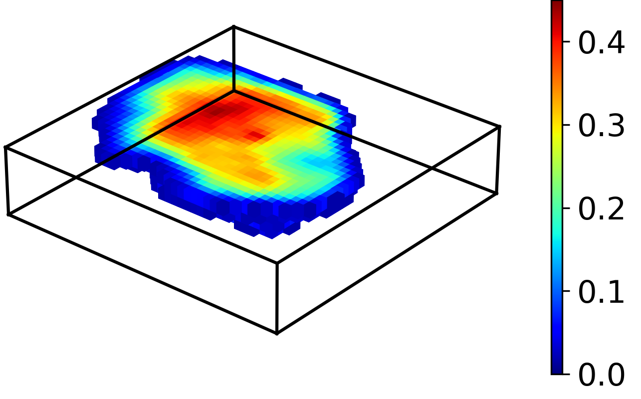
(j) 10 months (surr)

Figure 9: Comparison of time evolution between surrogate model predictions (surr) and reference simulation results (sim) for interpreted seismic saturation fields (Realization 2).

5.2.2 Monitoring data surrogate evaluation

The surrogate model for monitoring well data, described in Section 3.2, is trained to predict vertically resolved CO₂ saturation at 16 time steps (time steps 0, 2, 4, 6, $\ldots$, 30), one of which is the initial condition. The network contains 16 output channels, with each channel predicting saturation at a particular time step. For training, the batch size is set to 10, the model is trained for 150 epochs, and the initial learning rate is 0.001. This model requires only about 15 minutes for training on a Nvidia A100 GPU. Training is very fast in this case because this surrogate uses only local geomodel properties as inputs rather than the entire field, and it predicts saturations only for a single column of grid blocks (at 16 time steps).

Figure 10 shows the comparison between the predicted and true CO₂ saturation profiles at the monitoring well over time for three new randomly selected test-case realizations. The columns in each figure represent a single time step, and results are shown for all 35 layers in the model. We see very different behaviors in the three realizations – fairly uniform arrival times and saturation distributions in Realization 6, somewhat less uniformity in Realization 4, and a very localized saturation peak in Realization 5. For Realization 5, CO₂ has arrived at the monitoring well in only a few layers. Despite the high degree of variability between realizations, the surrogate model provides predictions in close visual agreement with reference simulation results in all cases.

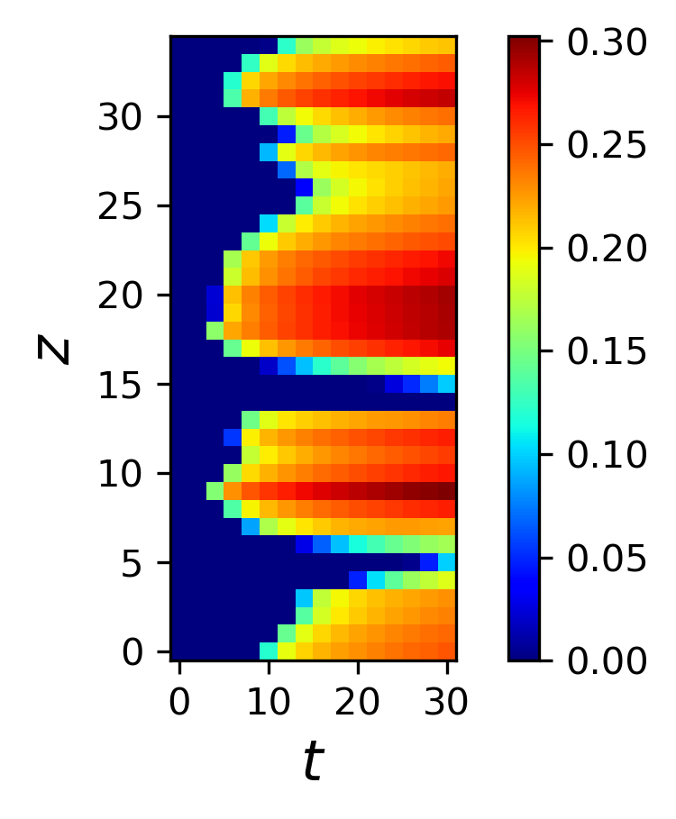
(a) Realization 4 (sim)

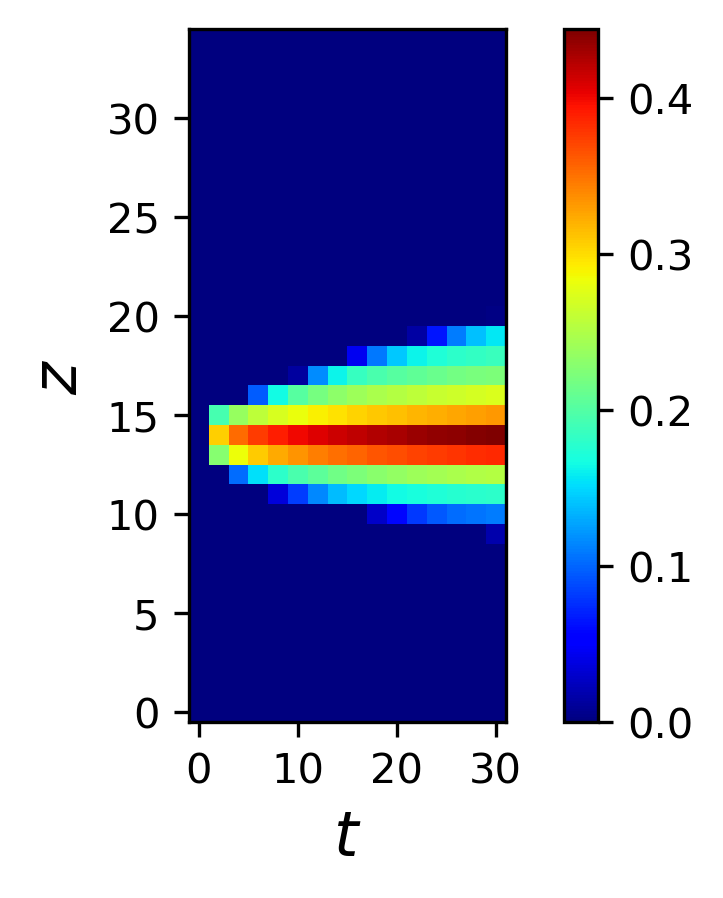
(b) Realization 5 (sim)

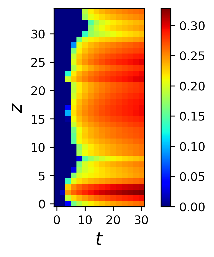
(c) Realization 6 (sim)

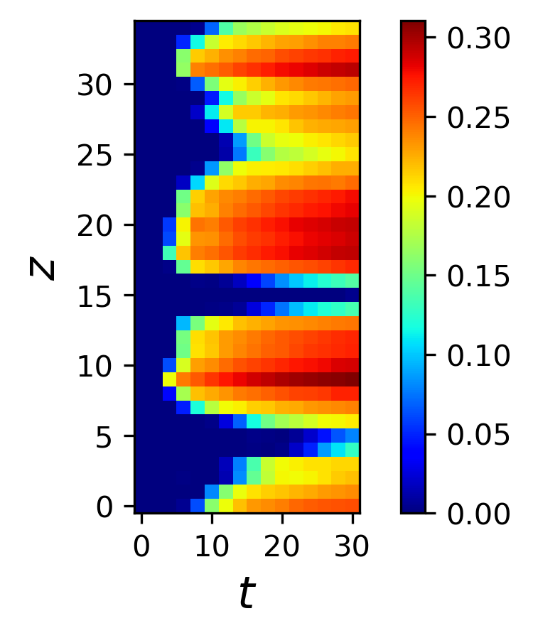
(d) Realization 4 (surr)

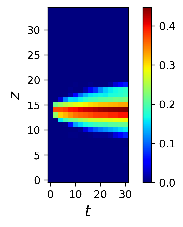
(e) Realization 5 (surr)

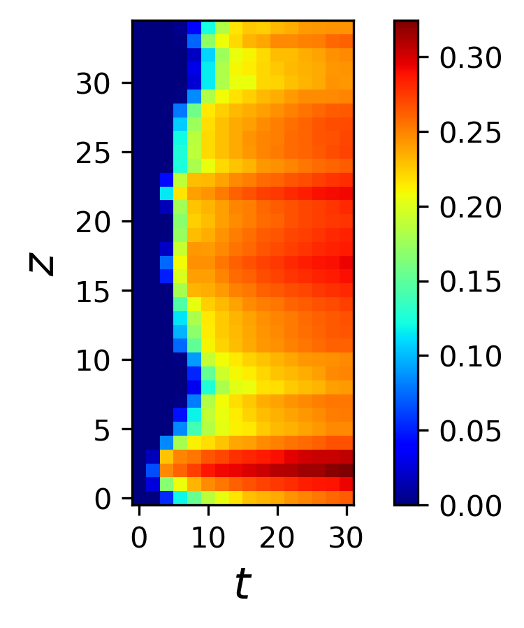
(f) Realization 6 (surr)

Figure 10: Comparison of time evolution between monitoring well surrogate saturation predictions (surr) and reference simulation results (sim) for three realizations. Each column corresponds to one of the 16 time steps considered.

It is useful to quantify the level of agreement between reference results and surrogate model predictions. To accomplish this, we compute the saturation mean absolute error (MAE, denoted as $\delta_{s}$) between the two sets of results as follows:

$$\delta_{s}=\frac{1}{n}\sum_{i=1}^{n}\lvert S_{i}-\hat{S}_{i}\rvert,$$ (12)

where $S_{i}$ and ${\hat{S}}_{i}$ denote the reference and surrogate model prediction, respectively, and $n$ is the total number of contributions to $S_{i}$ and ${\hat{S}}_{i}$. For the seismic surrogate we have $n=6\times 42\times 42\times 7=74,088$, and for the monitoring well surrogate model $n=16\times 35=560$. These errors are computed for each test case.

The MAEs for both the interpreted seismic surrogate and the monitoring well surrogate, over the 500 test-case realizations, are shown as box plots in Figure 11. In the box plots, the top and bottom of the box represent the 75th and 25th percentile (P₇₅ and P₂₅) errors and the lines outside the boxes represent the 90th and 10th percentile errors. The red lines inside the boxes correspond to the median error. These value are 0.00384 and 0.0155 for interpreted seismic data and monitoring well data, respectively. These low error values suggest that the surrogate models are sufficiently accurate for use in history matching.

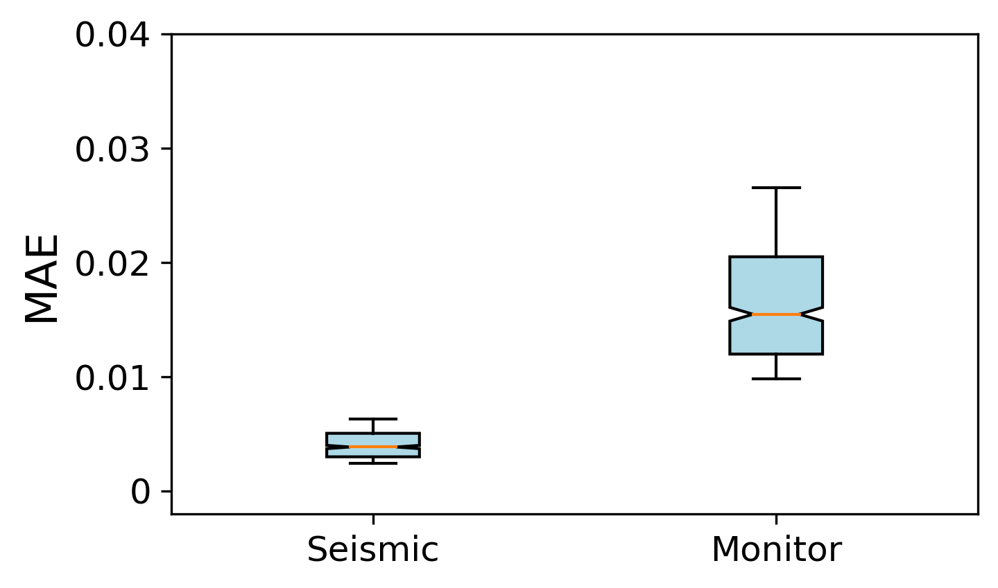
Figure 11: Box plots of mean absolute saturation errors for interpreted seismic surrogate (Seismic) and monitoring well surrogate (Monitor) over 500 test-case models.

6 Use of surrogate models for history matching

Here we first describe the problem setup, our treatment of the various error components appearing in the history matching formulation, and the representations used for the likelihood function. History matching results using the hierarchical MCMC procedure, with the deep learning surrogates applied for all forward simulations, are then presented.

6.1 Setup, errors and likelihood function

The true (synthetic) geomodel, used to provide observed data, is a realization characterized by the following metaparameter values: $\mu_{\log k}=3.0$, $\sigma_{\log k}=2.3$, $\log_{10}a_{r}=-1.8$ ($a_{r}=0.016$), $d=0.03$ and $e=0.055$. The true-model response for CO₂ saturation, along $y$-$z$ and $x$-$z$ cross sections through the injection well at a time of 1 year, is presented in Figure 12(a) and (b). The corresponding filtered seismic interpretations are displayed in Figure 12(c) and (d). The filtered response loses some of the detail, but the heterogeneity-driven channeling features still appear.

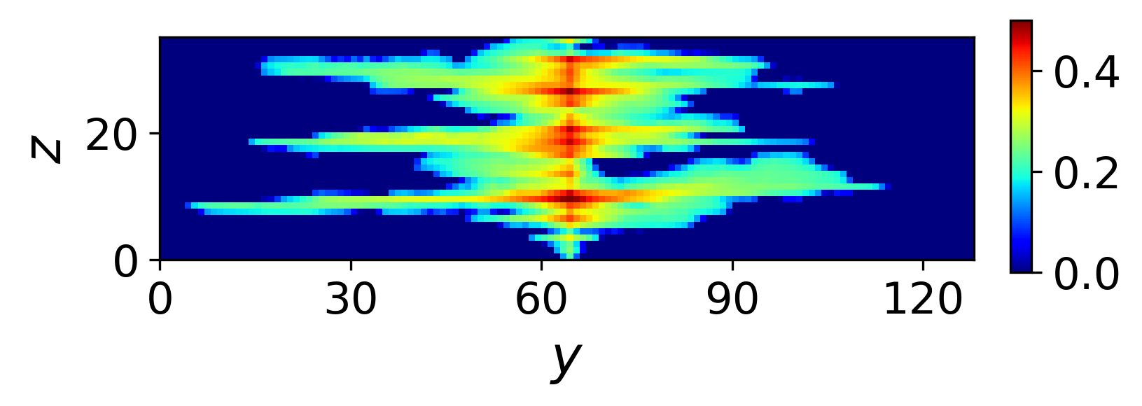
(a) High-fidelity $y$-$z$ cross section

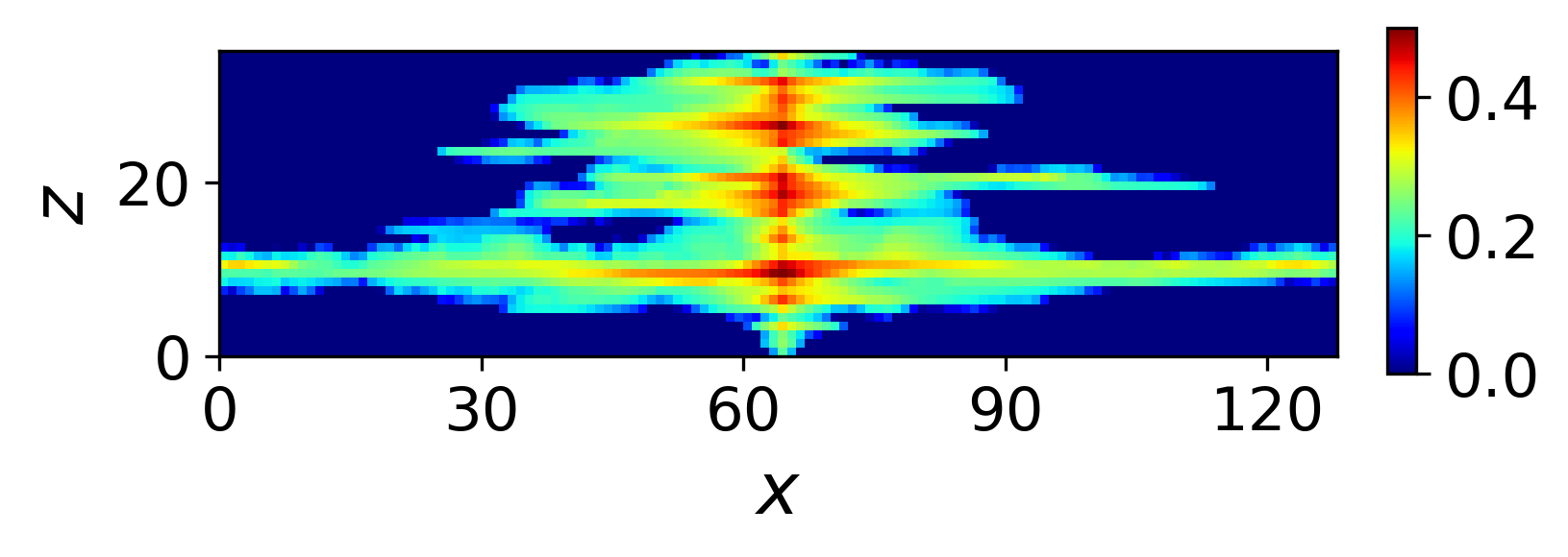
(b) High-fidelity $x$-$z$ cross section

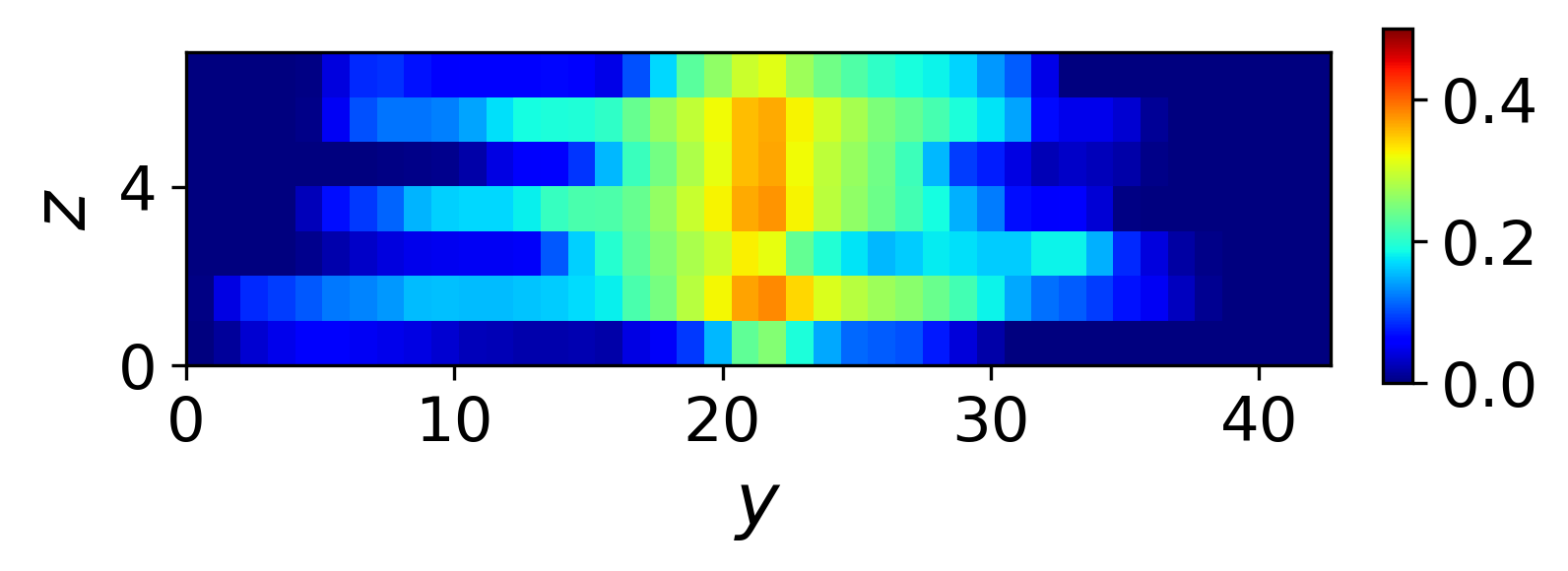
(c) Filtered $y$-$z$ cross section

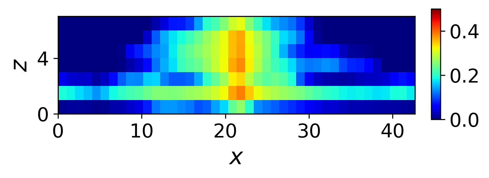
(d) Filtered $x$-$z$ cross section

Figure 12: True-model saturation fields at 1 year. Top row shows high-fidelity results for cross sections through the injection well, and bottom row shows corresponding filtered (interpreted seismic) results.

Noise, intended to represent measurement error, model resolution error, and surrogate approximation error, is added to the true data. The observed data vector is thus expressed as:

$$\mathbf{d}_{\text{obs}}=\mathbf{d}_{\text{true}}+\boldsymbol{\epsilon},$$ (13)

where $\boldsymbol{\epsilon}$ denotes all sources of noise. Here we take $\boldsymbol{\epsilon}$ to be uncorrelated and unbiased, i.e., of zero mean and diagonal covariance matrix. The measurement error and model resolution error are assigned directly in this work. For the monitoring well data, the standard deviation of the combined measurement and model resolution errors is set to be 5% of the maximum of the collected monitoring data over all available time steps. In our case this is 0.0162, which is close to the value (0.02) used by Sun and Durlofsky (2019). For the interpreted seismic data, the standard deviation of the error is set to be 10% of the maximum of the observed data over all available time steps. This is similar to the approach used by Gervais and Roggero (2010), who set the standard deviation of error to be 10% of the seismic data mean.

The surrogate-model approximation error ($\boldsymbol{\epsilon}_{\text{surr}}$) is calculated during the test-set evaluation. Specifically,

$$\boldsymbol{\epsilon}_{\text{surr}}=\mathbf{d}_{\text{pred}}-\mathbf{d}_{\text{true}},$$ (14)

where $\mathbf{d}_{\text{pred}}$ and $\mathbf{d}_{\text{true}}$ denote data predicted by the surrogate and true models, respectively. In our case, the mean and standard deviation of error in the monitoring data surrogate are 0.00124 and 0.0370, respectively. For the seismic surrogate, these values are -0.0001 and 0.0133, respectively. Thus we see that the average errors are near zero, consistent with the assumption of unbiased errors. The total standard deviation ($\sigma_{\text{total}}$), which combines the standard deviation of $\boldsymbol{\epsilon}_{\text{surr}}$ ($\sigma_{\text{surr}}$) and the measurement and model resolution errors (we denote the standard deviation of these two errors as $\sigma_{\text{d}}$), can then be obtained via $\sigma_{\text{total}}=\left(\sigma_{\text{surr}}^{2}+\sigma_{\text{d}}^{2}\right)^{1/2}$. The noise for the interpreted seismic data is added to the ‘true’ high-fidelity simulation results before the filtering procedure, consistent with the approach used by Bukshtynov et al. (2015). Note that other treatments for error can be readily incorporated into our framework. An approach that might be considered is one in which error varies as a function of saturation value, as could be the case if seismic data are more sensitive in some saturation ranges than others.

We will apply the hierarchical MCMC method introduced in Section 4 for cases involving both monitoring data and seismic data, and for cases involving only monitoring data. This will allow us to assess the impact of seismic data on uncertainty reduction. In the former case, the likelihood appearing in Eq. 10 and Eq. 11 is given by

$$\begin{split}p(\mathbf{d}_{\text{obs}}\mid\boldsymbol{\xi},\mathbf{h})=c\exp\left(\frac{1}{T}\left(-\frac{1}{2}(\mathbf{d}_{\text{obs}}^{\text{mon}}-f_{\text{mon}}(\boldsymbol{\xi},\mathbf{h}))^{T}C_{\text{mon}}^{-1}(\mathbf{d}_{\text{obs}}^{\text{mon}}-f_{\text{mon}}(\boldsymbol{\xi},\mathbf{h}))\right.\right.\\ \left.\left.-\frac{1}{2}(\mathbf{d}_{\text{obs}}^{\text{seis}}-f_{\text{seis}}(\boldsymbol{\xi},\mathbf{h}))^{T}C_{\text{seis}}^{-1}(\mathbf{d}_{\text{obs}}^{\text{seis}}-f_{\text{seis}}(\boldsymbol{\xi},\mathbf{h}))\right)\right),\end{split}$$ (15)

where $c$ is a normalization constant, $\mathbf{d}_{\text{obs}}^{\text{mon}}$ and $\mathbf{d}_{\text{obs}}^{\text{seis}}$ denote observed monitoring well data and interpreted seismic data, respectively, and $C_{\text{mon}}$ and $C_{\text{seis}}$ are the (diagonal) total error covariance matrices for monitoring well and seismic data, respectively. The quantity $T$ ($T>0$), referred to as simulated temperature, is a parameter that controls the acceptance rate of proposed samples (Li, 2012). If only the monitoring data are used for history matching, the seismic data portion of the likelihood does not appear, resulting in

$$\begin{split}p(\mathbf{d}_{\text{obs}}\mid\boldsymbol{\xi},\mathbf{h})=c\exp\left(\frac{1}{T}\left(-\frac{1}{2}(\mathbf{d}_{\text{obs}}^{\text{mon}}-f_{\text{mon}}(\boldsymbol{\xi},\mathbf{h}))^{T}C_{\text{mon}}^{-1}(\mathbf{d}_{\text{obs}}^{\text{mon}}-f_{\text{mon}}(\boldsymbol{\xi},\mathbf{h}))\right)\right).\end{split}$$ (16)

Additional parameter specifications are as follows. We set $\beta=0.05$, where $\beta$ (appearing in Eq. 9) scales the magnitude of sample updates. The standard deviation of the Gaussian proposal distribution for the metaparameters is set to be 0.05 of the parameter range. We specify $T=1$ when only monitoring data are used, and $T=5$ when both data types are used. These settings result in MCMC acceptance rates in the appropriate range, i.e., 10% to 40% (Gelman et al., 1996; Han et al., 2024). In the results below, hierarchical MCMC using only monitoring well data requires 47,569 function evaluations (18,749 models accepted). Results using both data types require 55,748 function evaluations (16,249 models accepted).

6.2 History matching results

For the history matching, we use monitoring well data at times of 24, 49, 73, 97 and 122 days and, in the case when it is considered, interpreted seismic data at 2 and 4 months. Results for later times are used to evaluate the predictions of the history matched models. Recall that the simulations proceed until a final time of 1 year.

Posterior results for the metaparameters, obtained from the last 10,000 accepted samples, for cases both with and without seismic data, are presented in Figures 13 and 14. The gray region in each figure represents the prior distribution of the metaparameter and the red dashed line indicates the true value of the metaparameter. The posterior histograms appear in blue for results in which only monitoring well data are used, and in orange for results where both monitoring well data and interpreted seismic data are used. A reasonable degree of uncertainty reduction is achieved for $\mu_{\log k}$, $\sigma_{\log k}$ and $\log_{10}a_{r}$ when only monitoring well data are used (Figure 13(a), (c) and (e)). In addition, it is evident that the mode of the posterior histogram is near the true value for these quantities.

Very little uncertainty reduction is observed for parameters $d$ and $e$ in this case (Figure 14(a) and (c)), indicating that the monitoring well data are not informative in terms of the relationship between $\phi$ and $\log k$. This is consistent with the observations of Han et al. (2024). Uncertainty reduction is achieved, however, in the porosity field itself. This is demonstrated in Figure 14(e), where we show the prior and posterior distributions for the mean of the porosity, $\mu_{\phi}$. The results in Figure 14(e) are determined by computing, in turn, the average porosity for 3000 randomly sampled prior and posterior realizations.

Considerably more uncertainty reduction in the key metaparameters is achieved when both monitoring well data and seismic data are used. Specifically, we observe narrower distributions, which include the true value, for $\mu_{\log k}$, $\sigma_{\log k}$ and $\log_{10}a_{r}$ (Figure 13(b), (d), (f)). There is also more uncertainty reduction in $d$ and $e$ in this case (Figure 14(b) and (d)), though significant posterior uncertainty in these quantities remains. As is apparent in Figure 14(f), the use of both data types provides substantial uncertainty reduction in mean porosity itself. Taken in total, the results in Figures 13 and 14 clearly show the additional (significant) uncertainty reduction achieved when interpreted seismic data are incorporated into the data assimilation procedure.

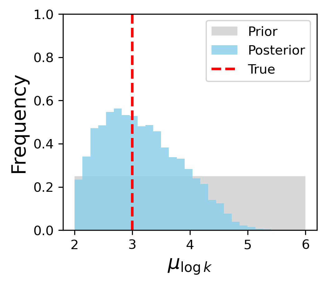
(a) $\mu_{\log k}$ without seismic

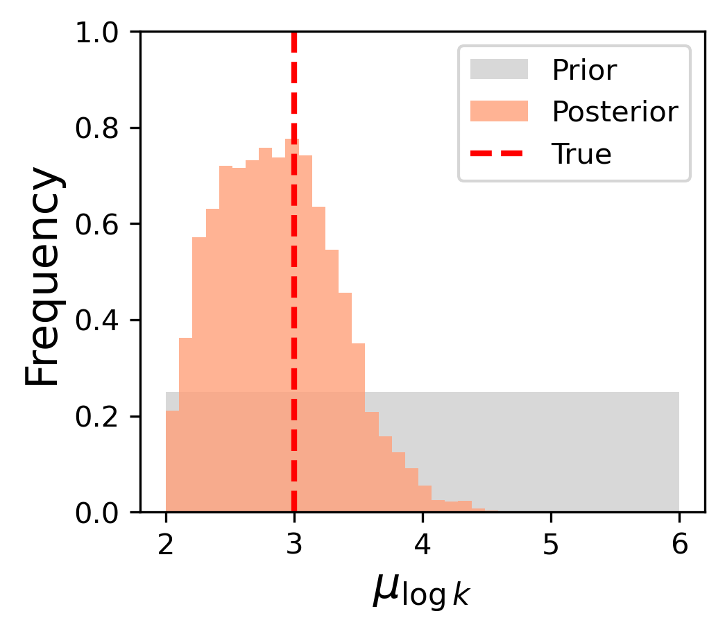
(b) $\mu_{\log k}$ with seismic

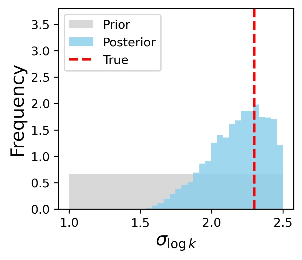
(c) $\sigma_{\log k}$ without seismic

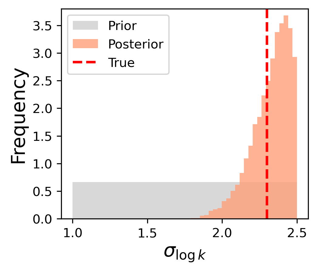
(d) $\sigma_{\log k}$ with seismic

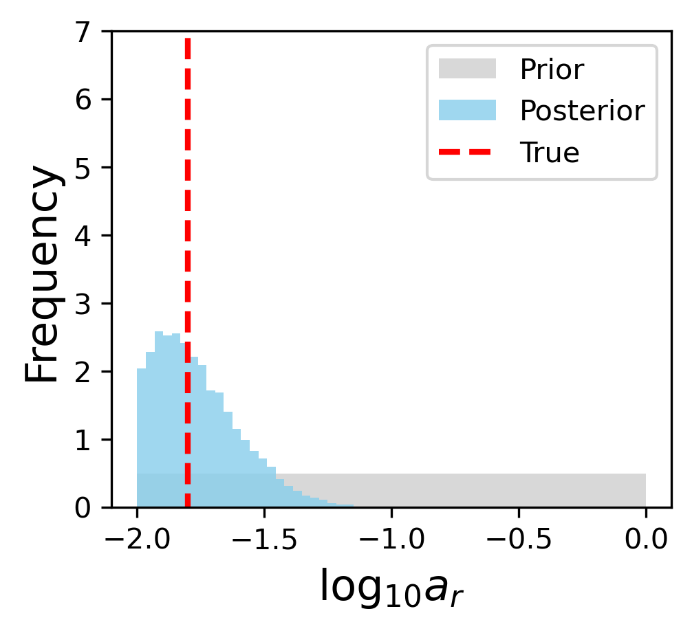
(e) $\log_{10}a_{r}$ without seismic

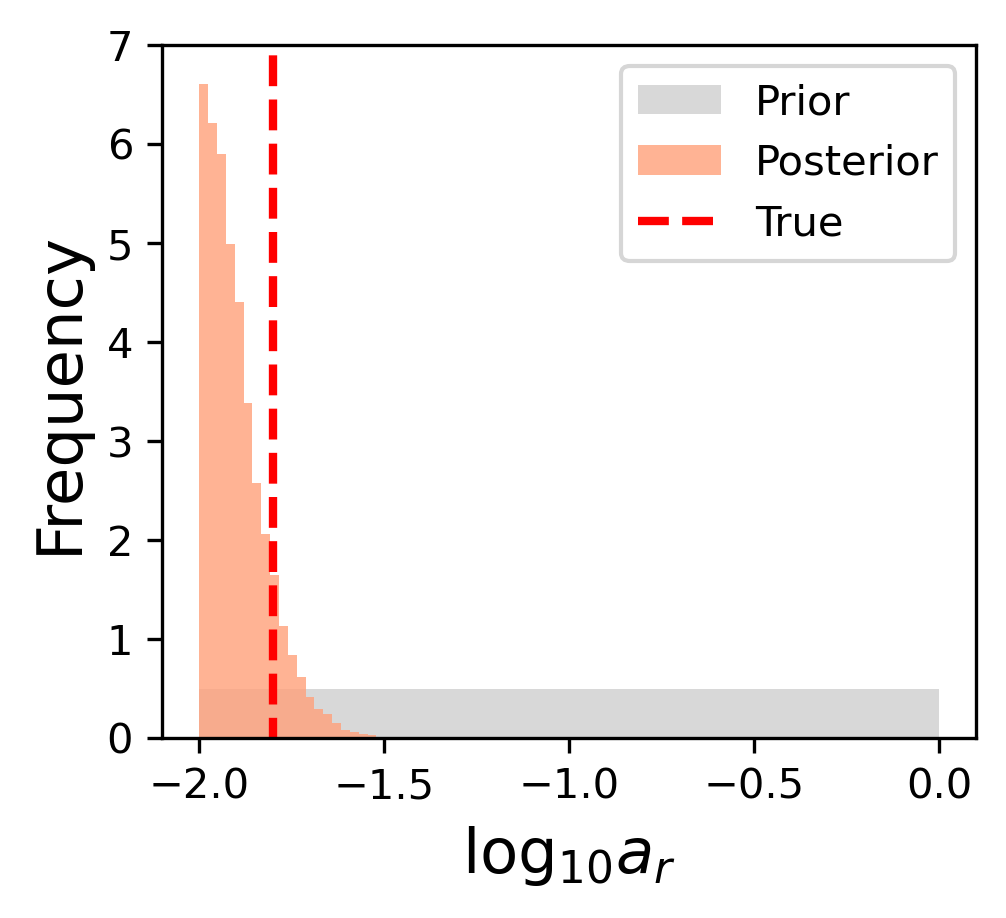
(f) $\log_{10}a_{r}$ with seismic

Figure 13: History matching results for metaparameters $\mu_{\log k}$, $\sigma_{\log k}$ and $\log_{10}a_{r}$ with monitoring well data only (left column, blue histograms) and with both monitoring well data and interpreted seismic data (right column, orange histograms). Priors shown in gray and true values indicated by the vertical red line.

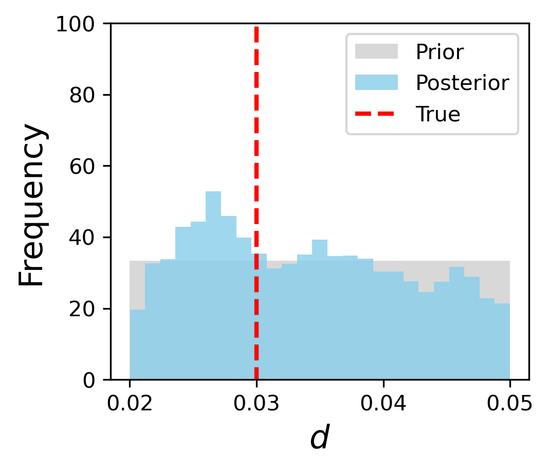
(a) $d$ without seismic

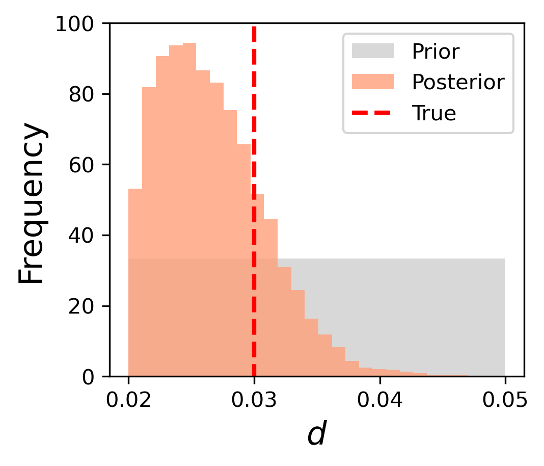
(b) $d$ with seismic

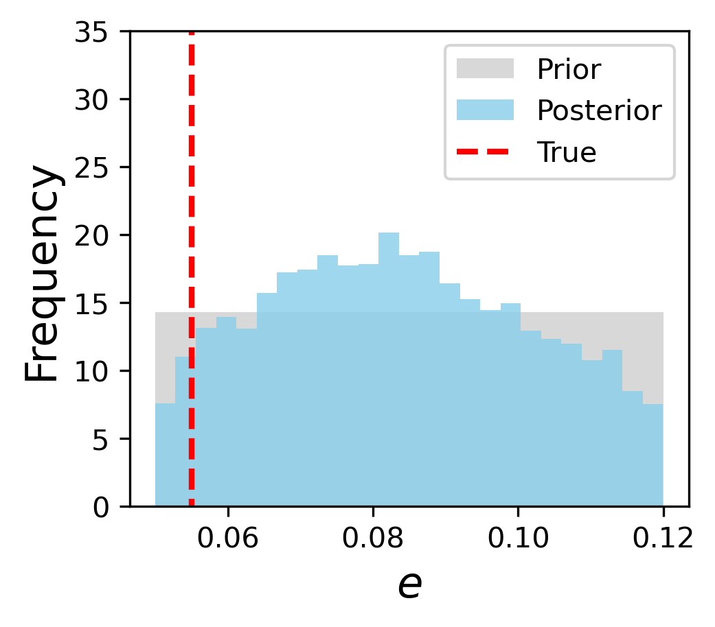
(c) $e$ without seismic

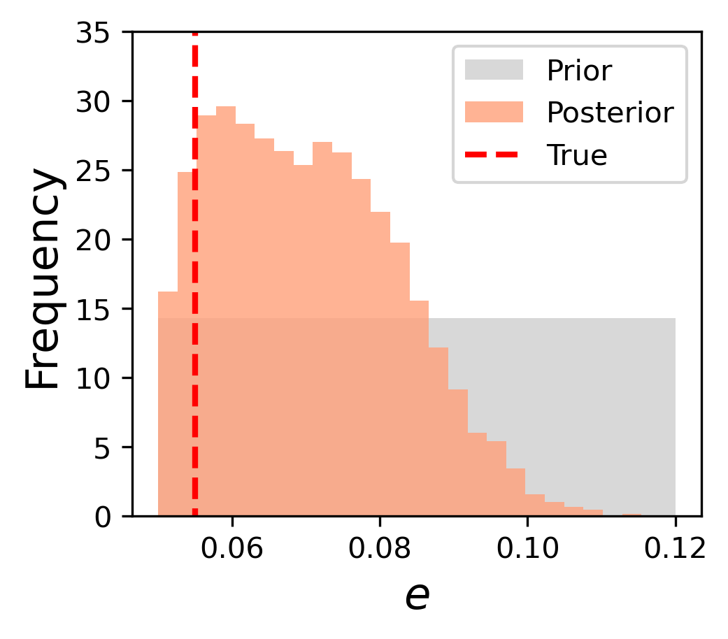
(d) $e$ with seismic

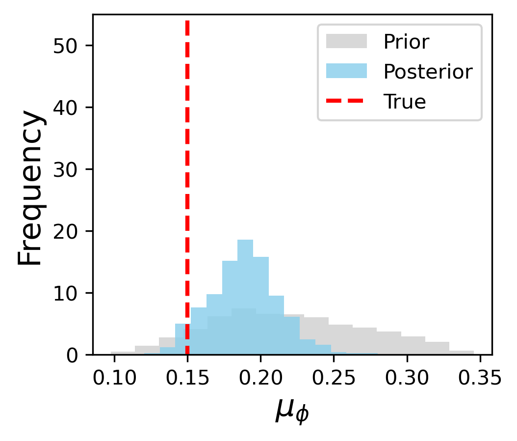
(e) $\mu_{\phi}$ without seismic

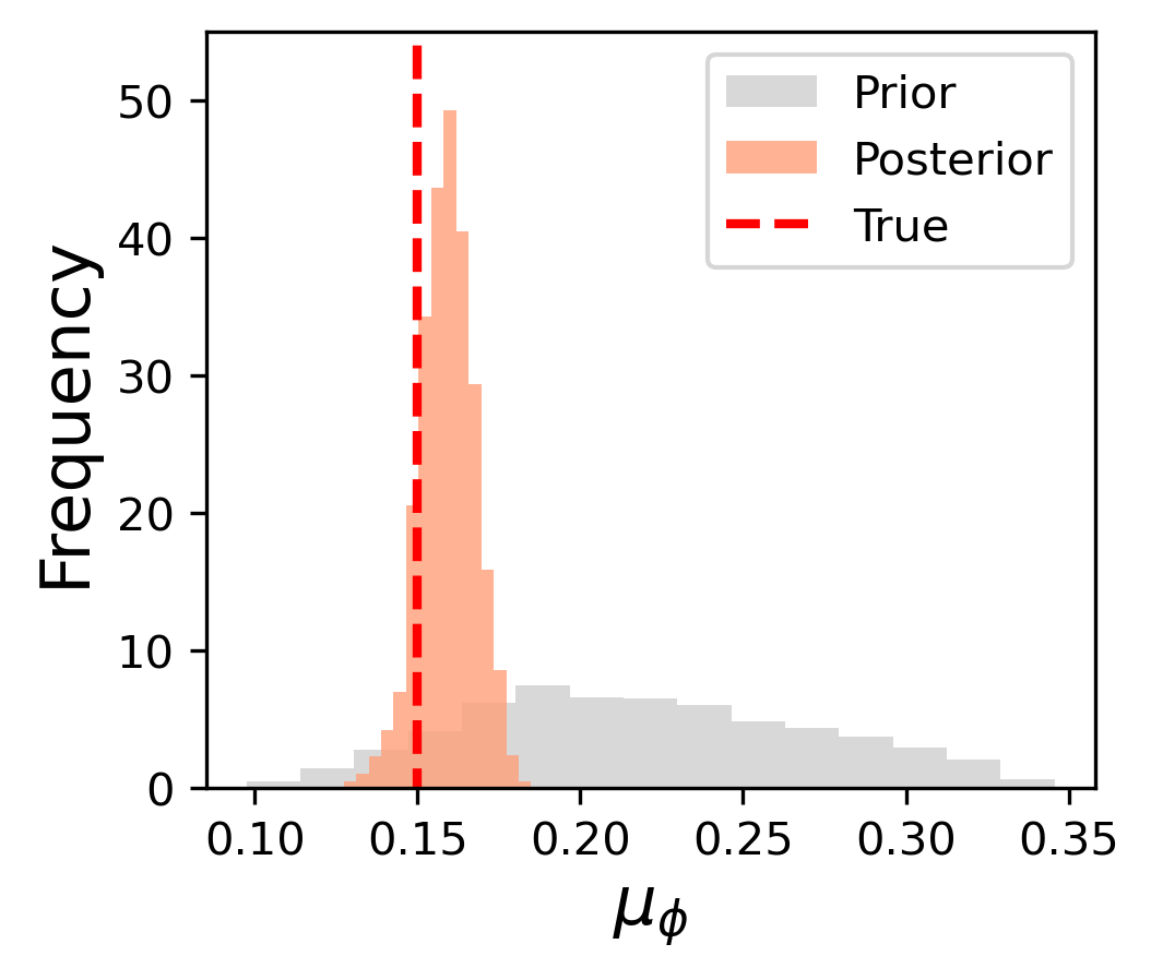
(f) $\mu_{\phi}$ with seismic

Figure 14: History matching results for metaparameters $d$ and $e$ and average porosity $\mu_{\phi}$ with monitoring well data only (left column, blue histograms) and with both monitoring well data and interpreted seismic data (right column, orange histograms). Priors shown in gray and true values indicated by the vertical red line.

We next present saturation fields (CO₂ plumes) for prior and posterior geomodels. In order to identify ‘representative’ interpreted seismic saturation fields, and thus enable meaningful comparisons, we proceed as follows. We randomly select 1000 prior geomodel realizations from the training set, 1000 realizations from the geomodels accepted during history matching with only monitoring data, and 1000 realizations from the geomodels accepted during history matching with both data types. Interpreted seismic data are then generated for each of these 3000 realizations using the seismic surrogate model. Then, for each set of models (prior, history matching with monitoring data, history matching with both data types), we apply k-means clustering to construct four clusters. The medoid from each cluster is then viewed as a representative interpreted seismic saturation field.

The resulting 12 saturation fields are shown in Figure 15 ($y$-$z$ cross sections through the injection well) and in Figure 16 ($x$-$z$ cross sections through the injection well). These results are all at a time of 1 year. The true results for this case are shown in Figure 12(c) and (d). The plumes in the prior realizations are fairly regular, varying from near-cylindrical to cone-shaped. The plumes for the posterior models all differ considerably from any of the prior plumes, and all resemble the true result to some degree. Specifically, in both figures, the posterior plumes all display CO₂ channeling toward the bottom of the model. Posterior results in which both data types are used are closer to the true saturation fields. For example, in Figure 15(i)-(l) we see three somewhat distinct channels to the left of the injector along with CO₂ moving further to the left than the right. These behaviors, consistent with Figure 12(c), are not consistently observed in Figure 15(e)-(h). In addition, the extent of CO₂ channeling toward the bottom of the model is better captured in Figure 16(i)-(l) than in Figure 16(e)-(h) (compare to Figure 12(d)). These results reiterate the advantages of using both data types for history matching.

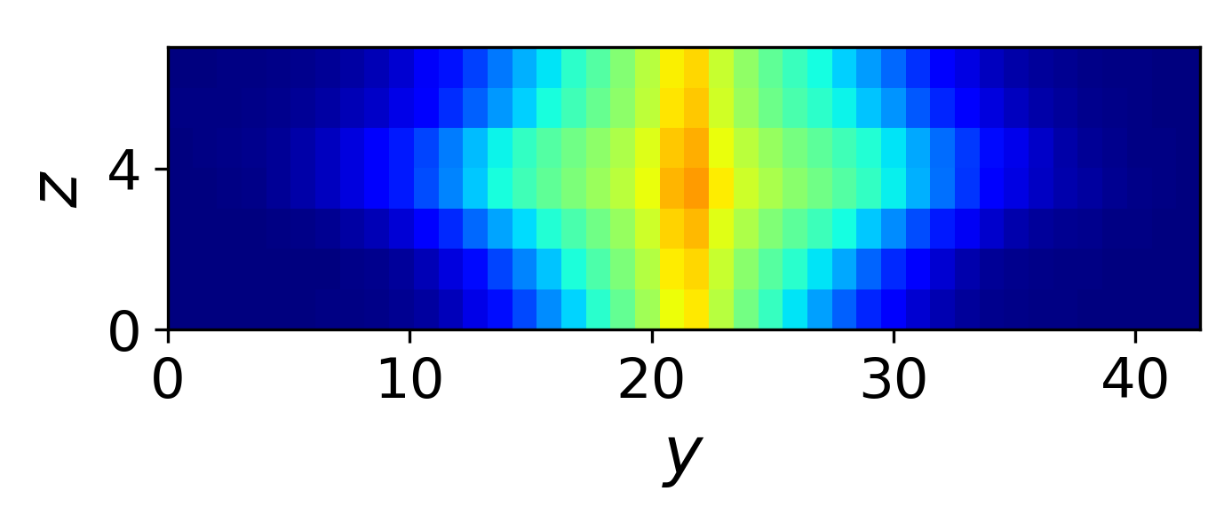
(a) Prior 1

(b) Prior 2

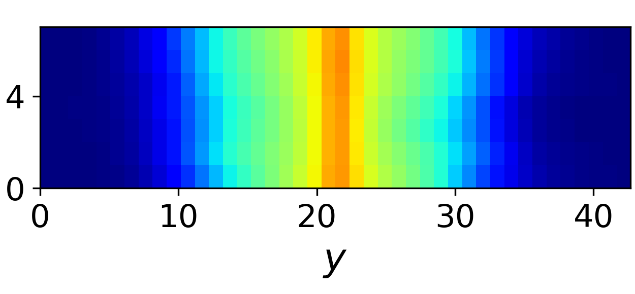
(c) Prior 3

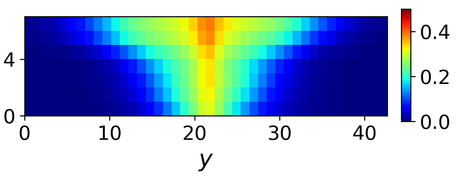
(d) Prior 4

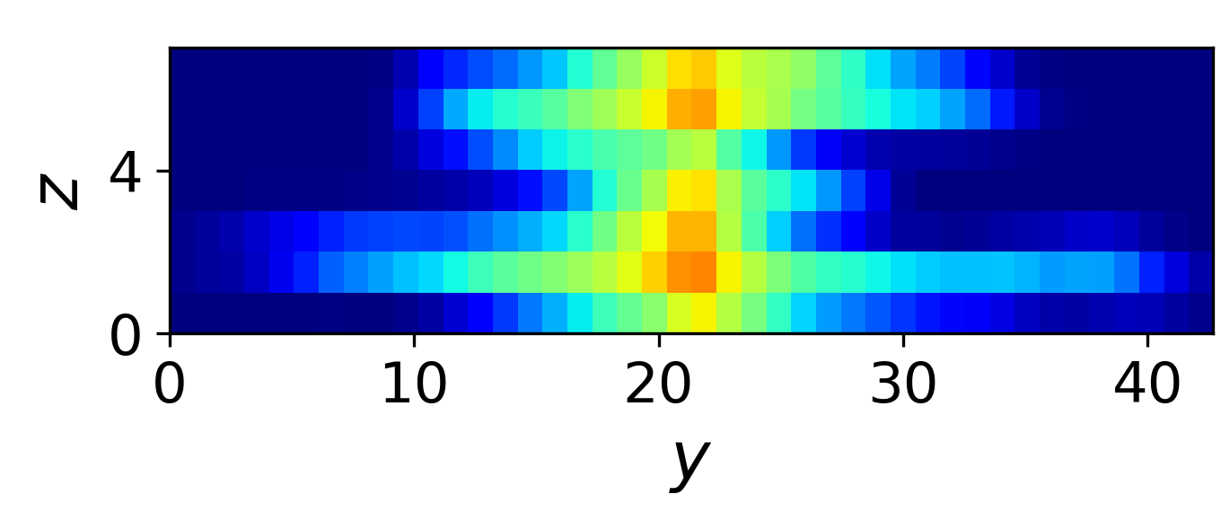
(e) Post. 1 (w/o seis)

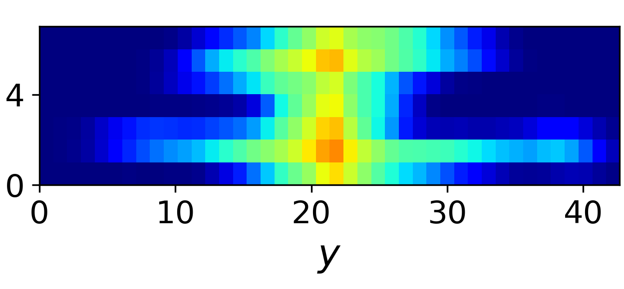
(f) Post. 2 (w/o seis)

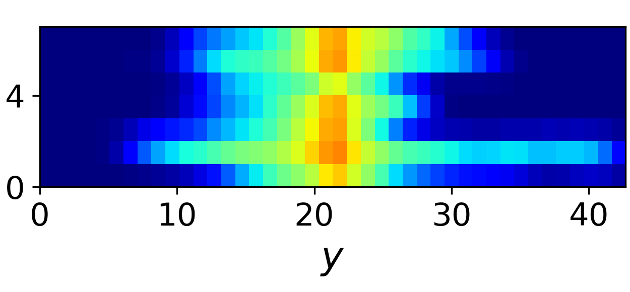
(g) Post. 3 (w/o seis)

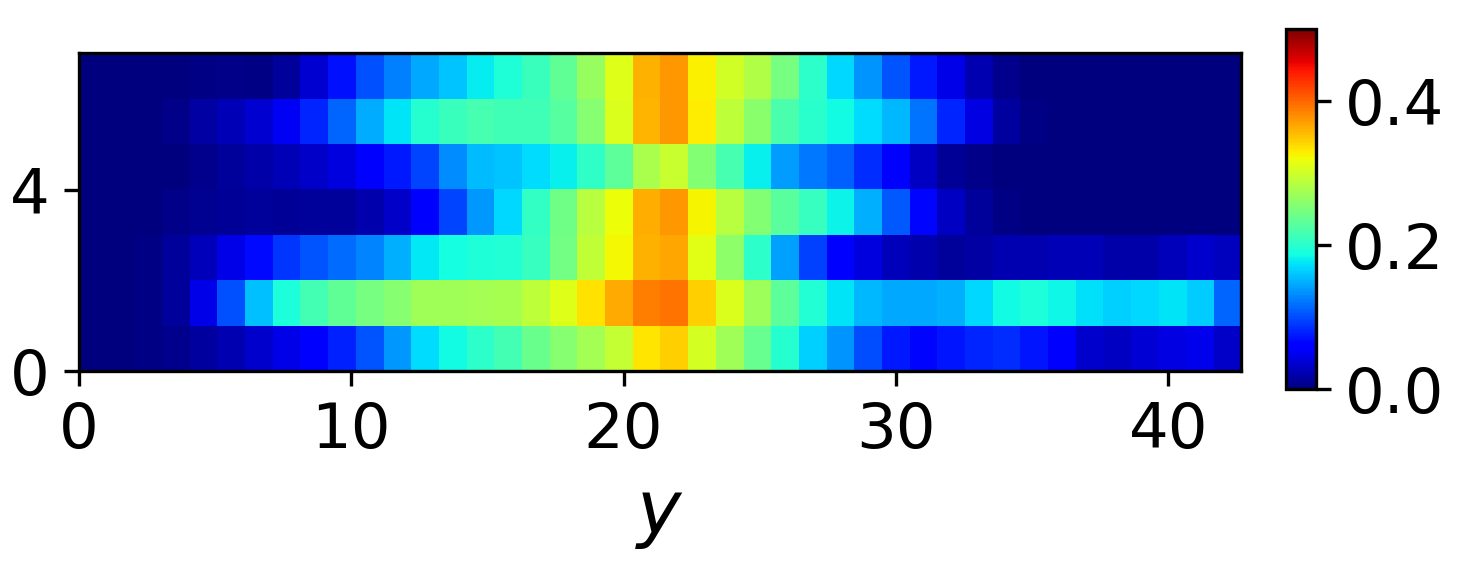
(h) Post. 4 (w/o seis)

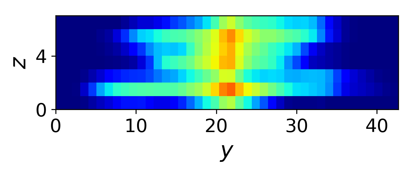
(i) Post. 1 (with seis)

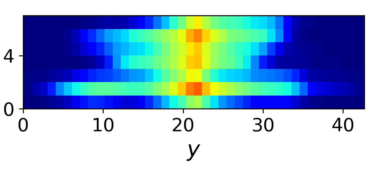
(j) Post. 2 (with seis)

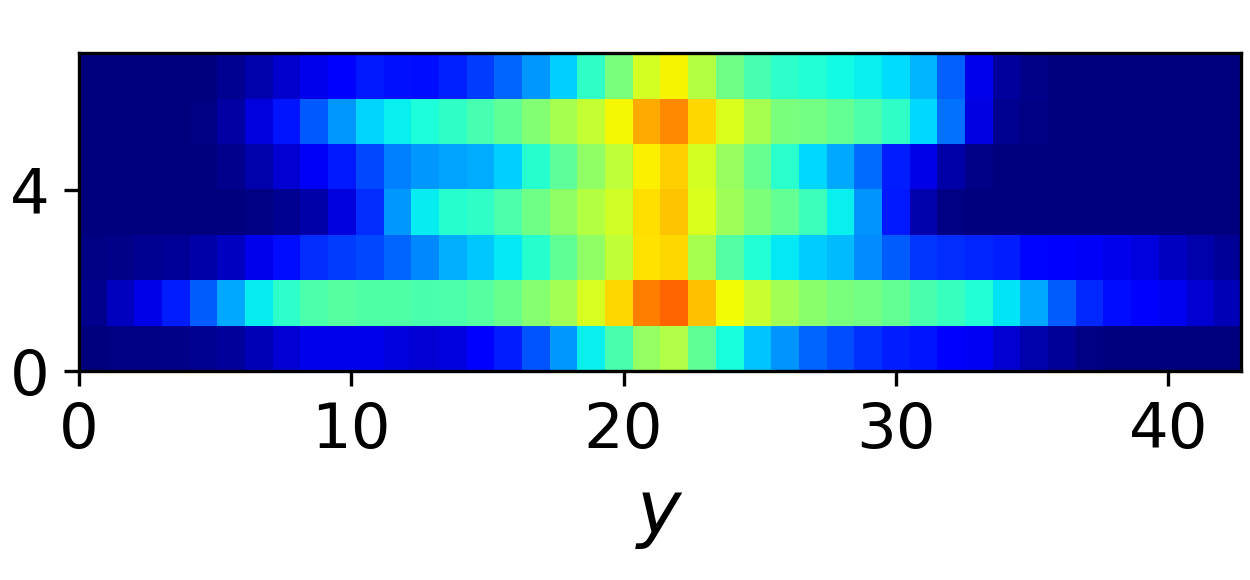
(k) Post. 3 (with seis)

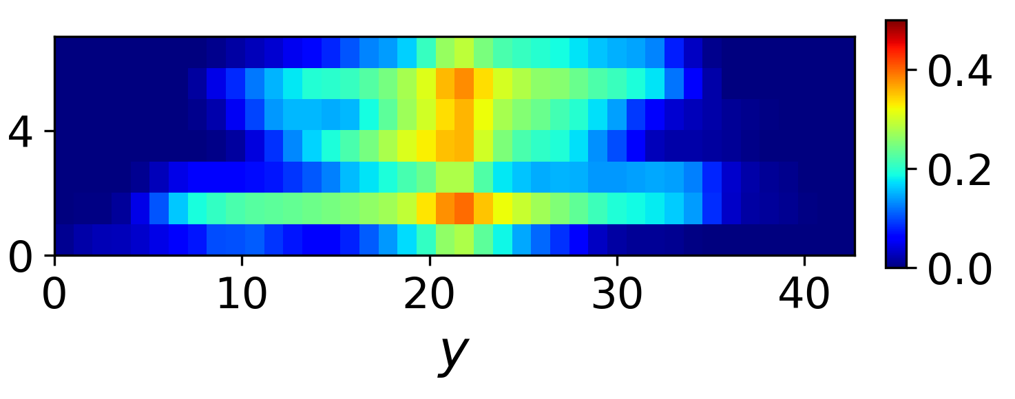
(l) Post. 4 (with seis)

Figure 15: Representative interpreted seismic saturation fields in $y$-$z$ cross sections through the injector at 1 year for prior realizations (first row), posterior realizations obtained using only monitoring well data (second row), and posterior realizations obtained using both monitoring well and seismic data (third row). True result shown in Figure 12(c).

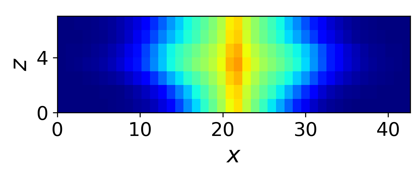
(a) Prior 1

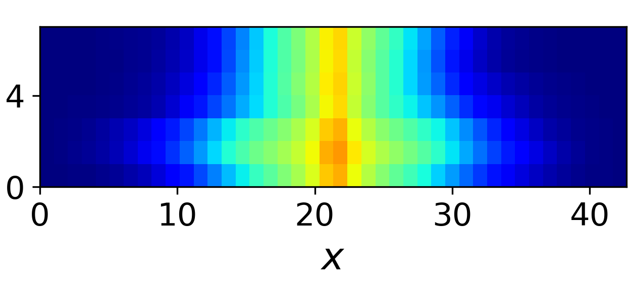
(b) Prior 2

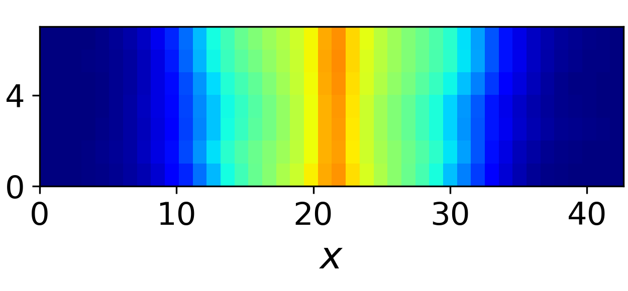
(c) Prior 3

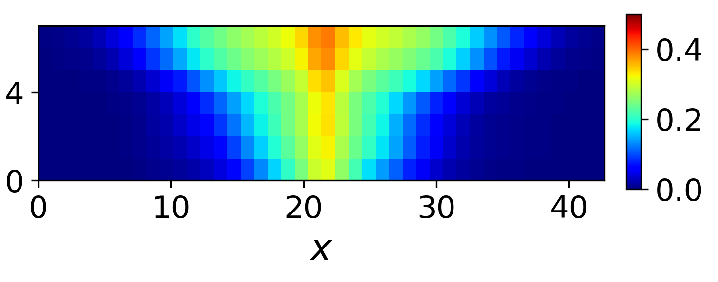
(d) Prior 4

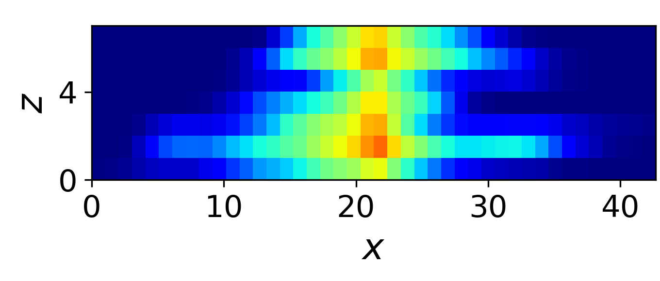
(e) Post. 1 (w/o seis)

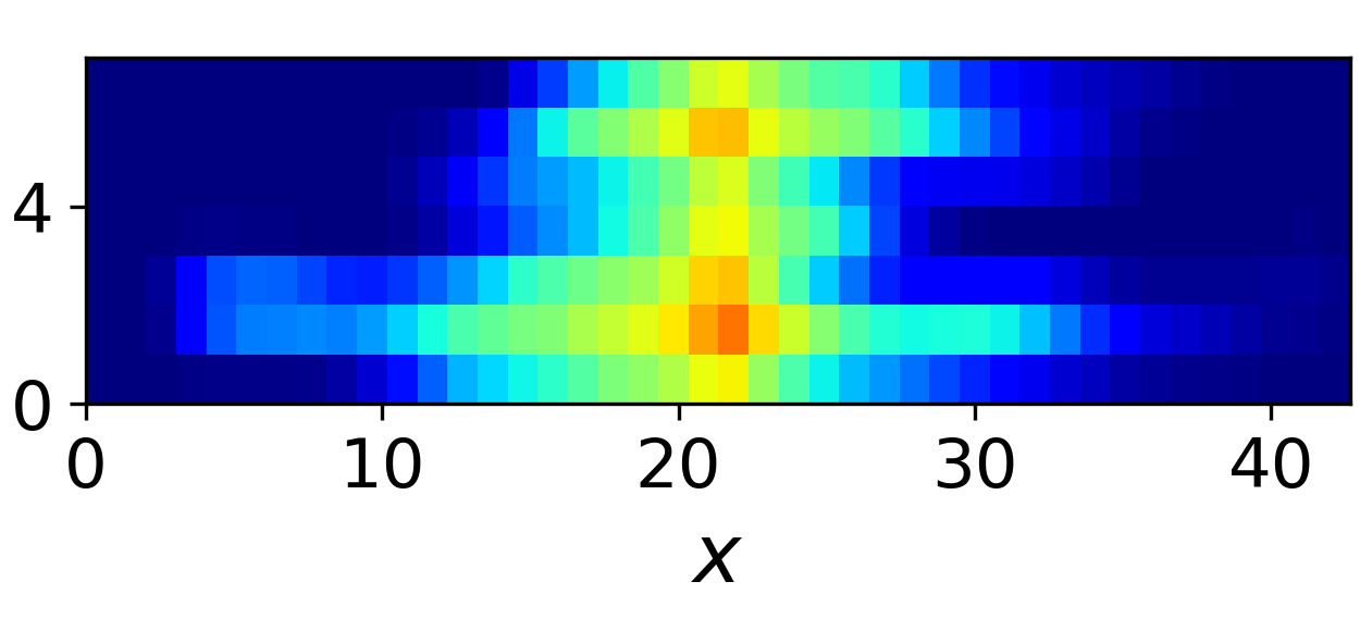
(f) Post. 2 (w/o seis)

(g) Post. 3 (w/o seis)

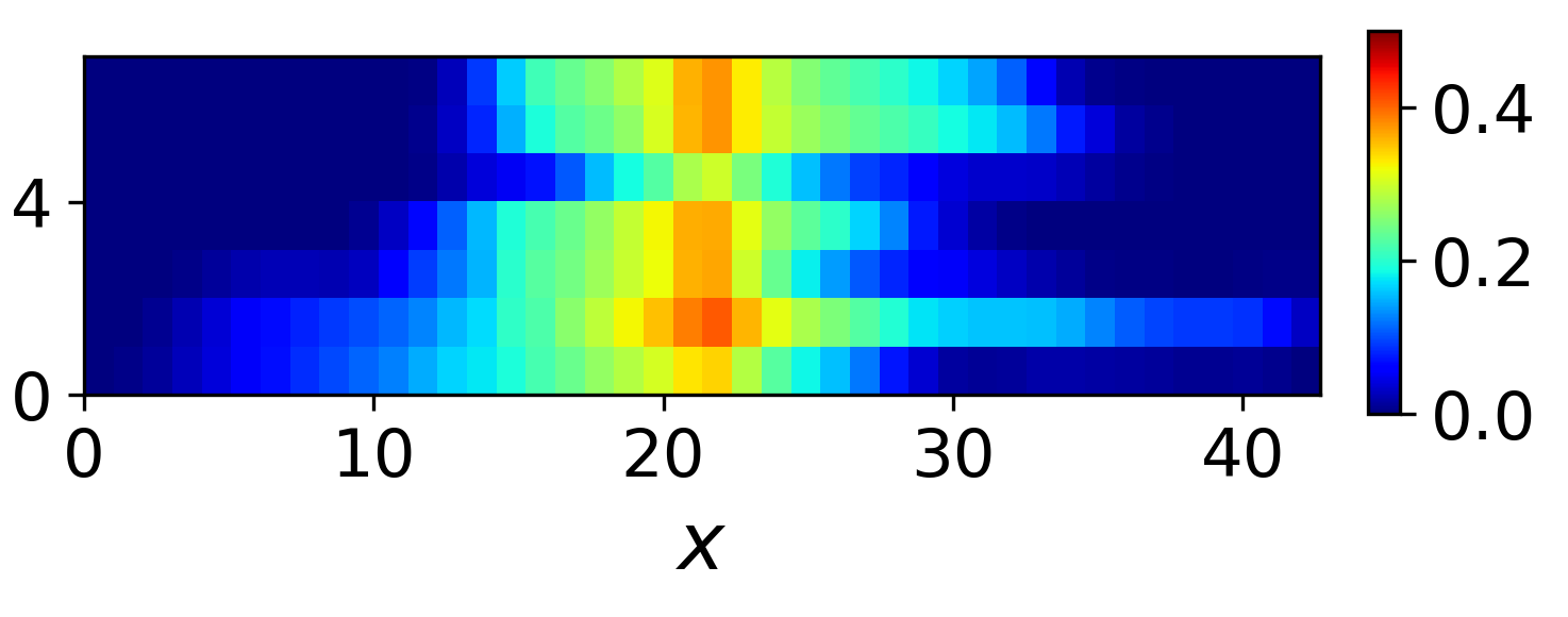
(h) Post. 4 (w/o seis)

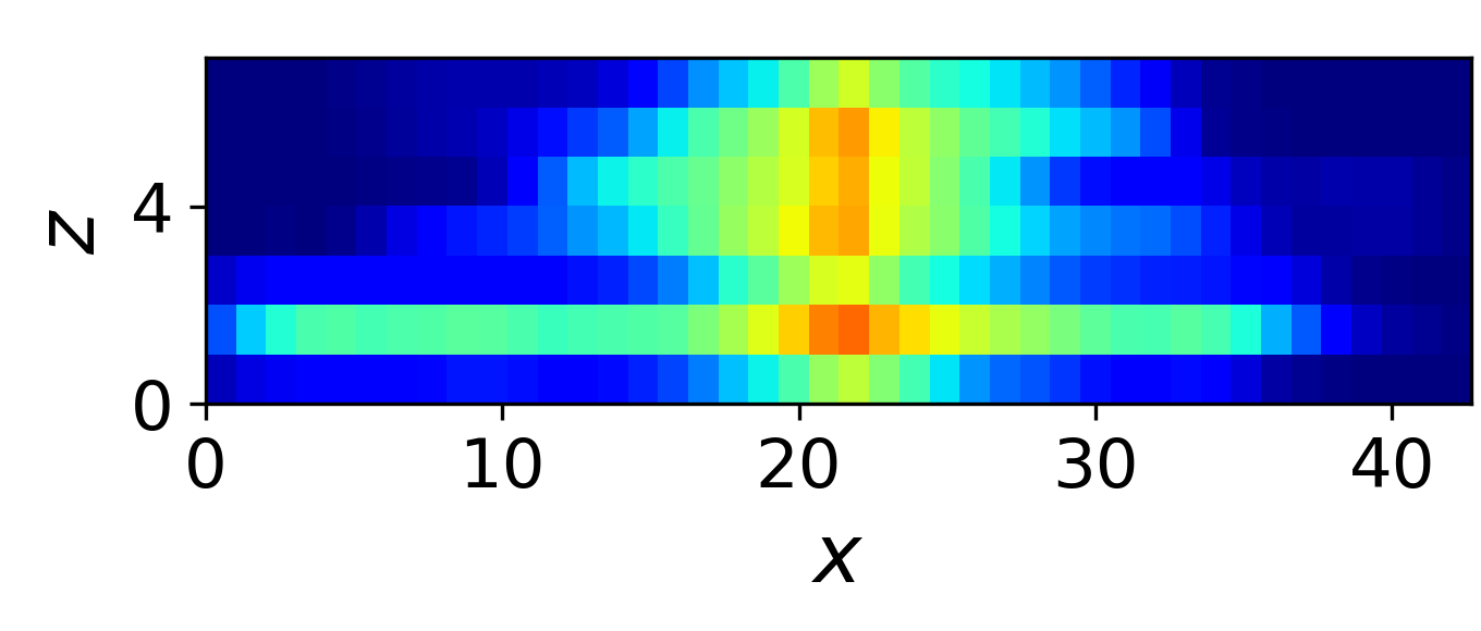
(i) Post. 1 (with seis)

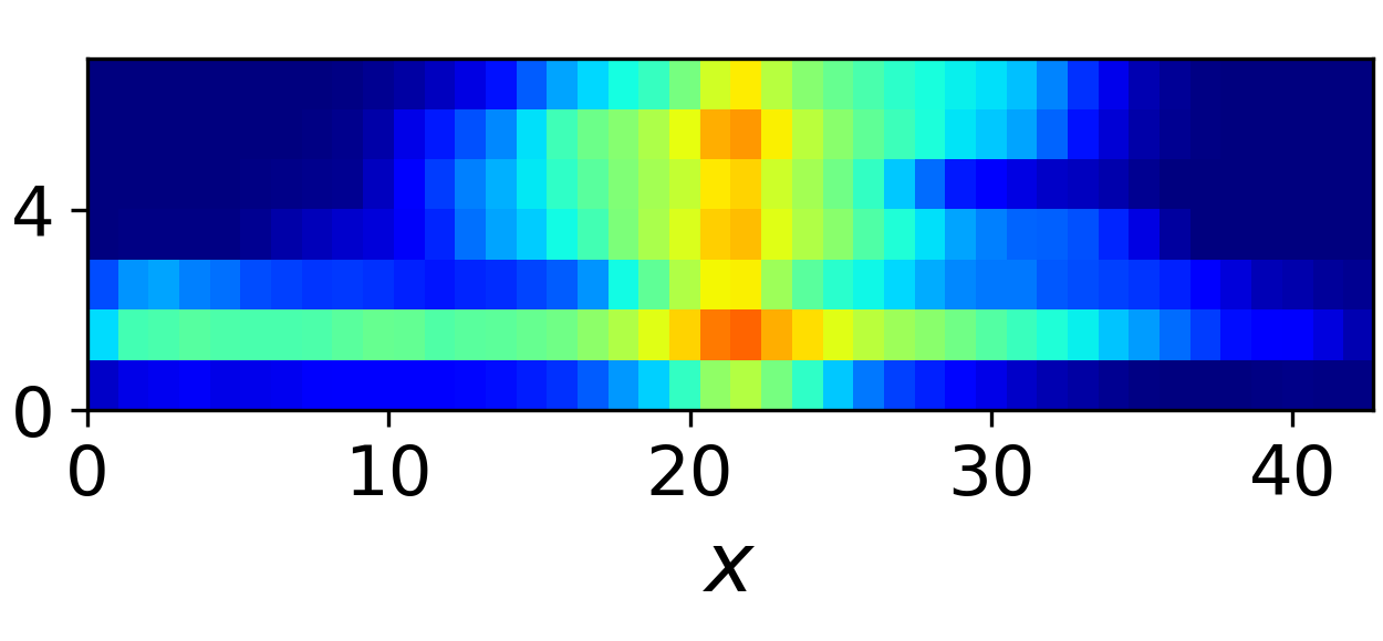
(j) Post. 2 (with seis)

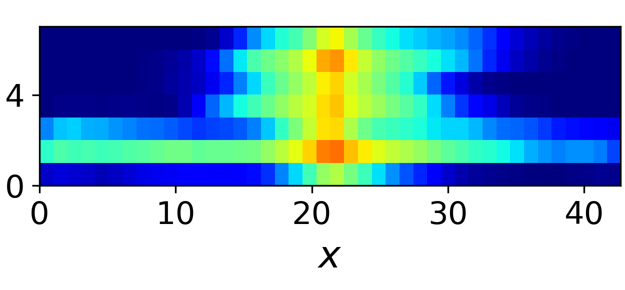
(k) Post. 3 (with seis)

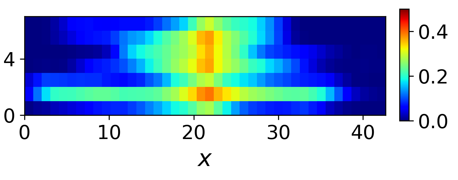
(l) Post. 4 (with seis)

Figure 16: Representative interpreted seismic saturation fields in $x$-$z$ cross sections through the injector at 1 year for prior realizations (first row), posterior realizations obtained using only monitoring well data (second row), and posterior realizations obtained using both monitoring well and seismic data (third row). True result shown in Figure 12(d).

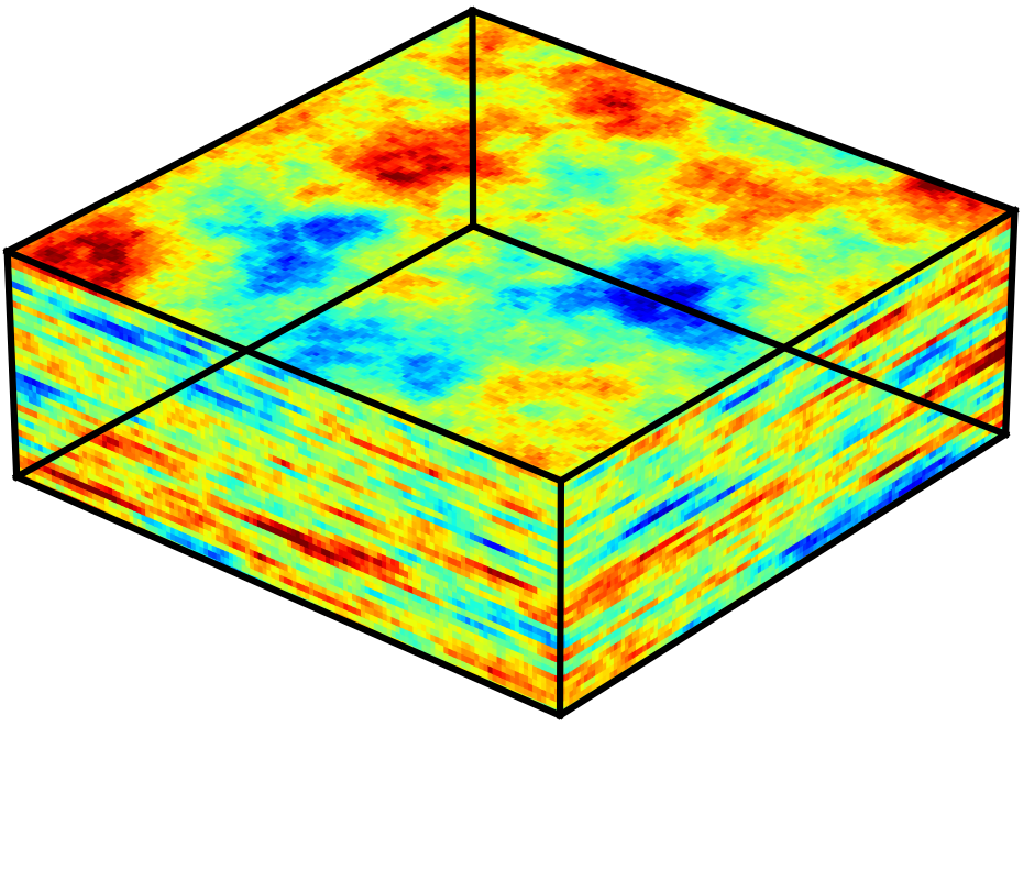
(a) True model

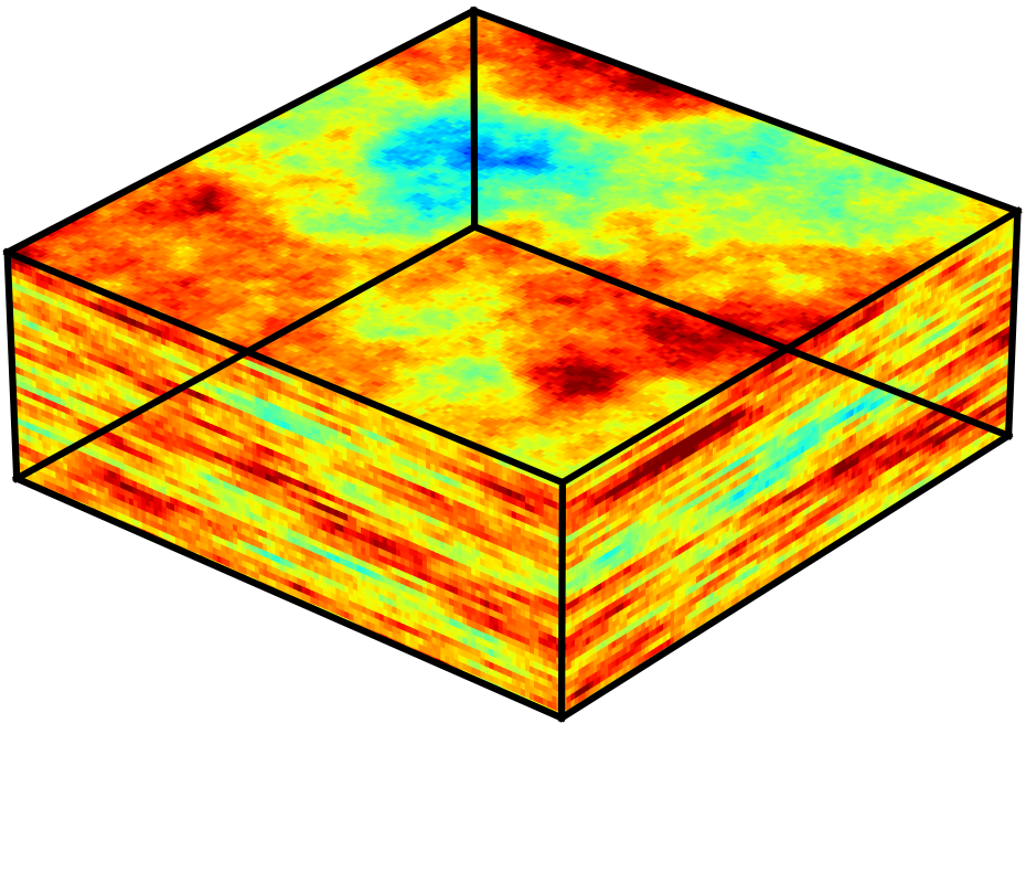
(b) Prior 1

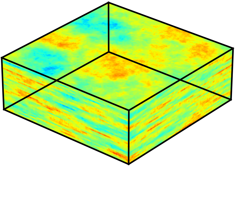
(c) Prior 2

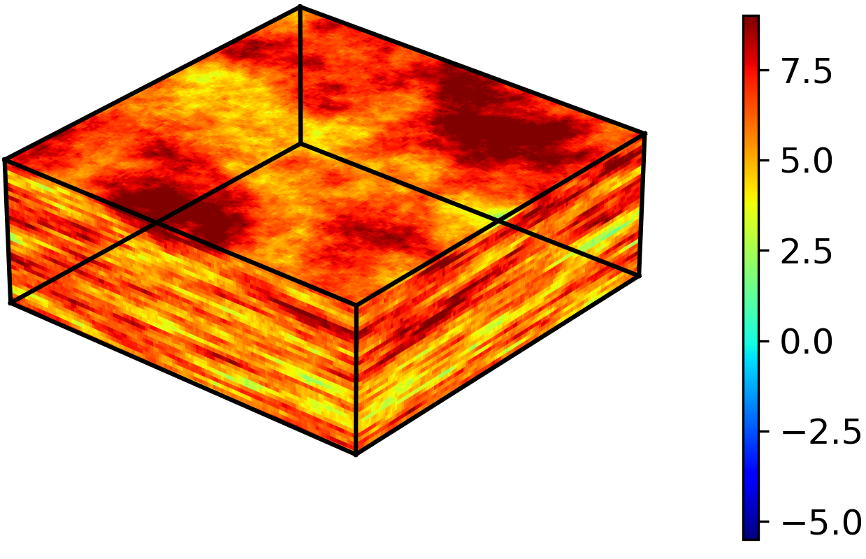
(d) Prior 3

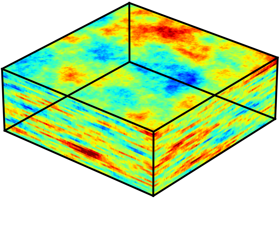
(e) Posterior 1

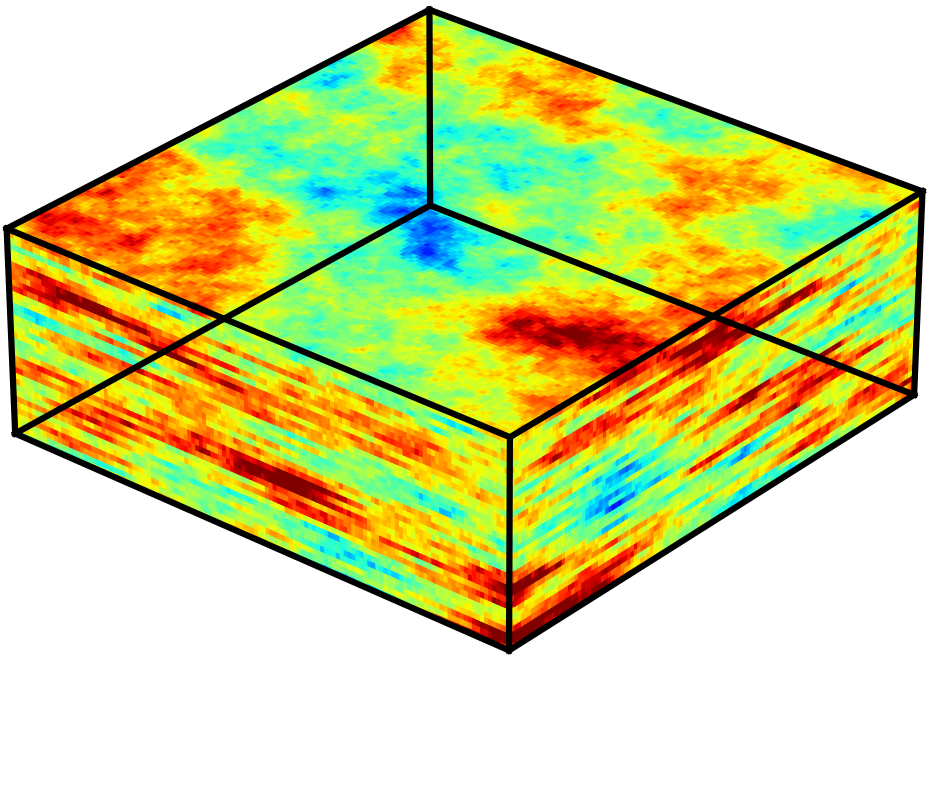
(f) Posterior 2

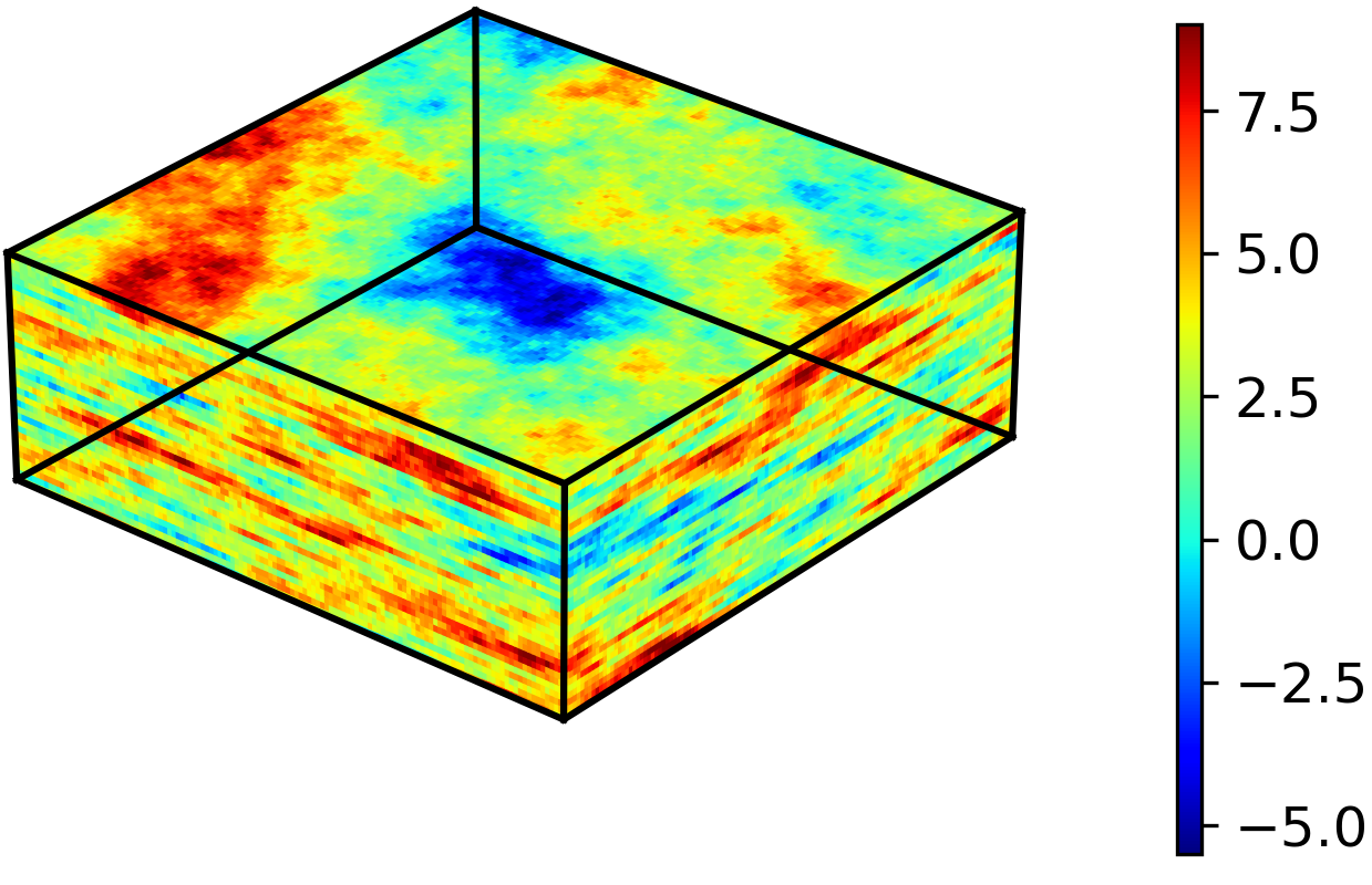
(g) Posterior 3

Figure 17: True model, three randomly sampled prior realizations, and three randomly sampled posterior realizations obtained using both monitoring well and interpreted seismic data. Geomodels shown in terms of $\log k_{x}$, with $k_{x}$ in md.

Although the posterior saturation fields shown in Figures 15 and 16 are at the coarse (interpreted seismic) scale, it is important to reiterate that our procedure provides high-resolution posterior geomodels. This is illustrated in Figure 17, where we display randomly sampled prior and posterior geomodel realizations ($\log k_{x}$ is the quantity displayed) along with the true model. The posterior models derive from history matching using both data types. It is evident that the three prior models show very different ranges for $\log k_{x}$, with notable scale variation between Prior 2 and Prior 3 (Figure 17(c) and (d)). The posterior realizations, by contrast, show similar ranges and variability in $\log k_{x}$, as well as general correspondence with the true model (Figure 17(a)). This is as expected since the posterior uncertainty in $\mu_{\log k}$ and $\sigma_{\log k}$ is relatively small.

As a final assessment of the applicability of the seismic surrogate model, we simulate the posterior realizations in Figure 17(e)-(g) and then apply the filtering procedure to obtain interpreted seismic results. Saturation fields at 1 year are shown in Figure 18. The upper two rows show $y$-$z$ cross sectional results from simulation and surrogate model predictions, and the lower two rows are analogous results for $x$-$z$ cross sections. As expected, all of these fields resemble, to some degree, the true results in Figure 12(c) and (d). There is also clear correspondence between the simulation results and the surrogate model results, though slight differences are evident.

We note finally that, if the surrogate model is not sufficiently accurate for predictions with posterior realizations, some amount of retraining could be performed. The new training realizations in this case would be generated by sampling from the posterior distributions of the metaparameters. The MCMC history matching would then be repeated, in this case with a surrogate model that is more accurate in the region of interest. Such a workflow would be quite manageable given the speed of the surrogate models used in this work.

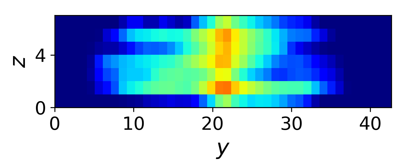
(a) Posterior 1 ($y$-$z$, sim)

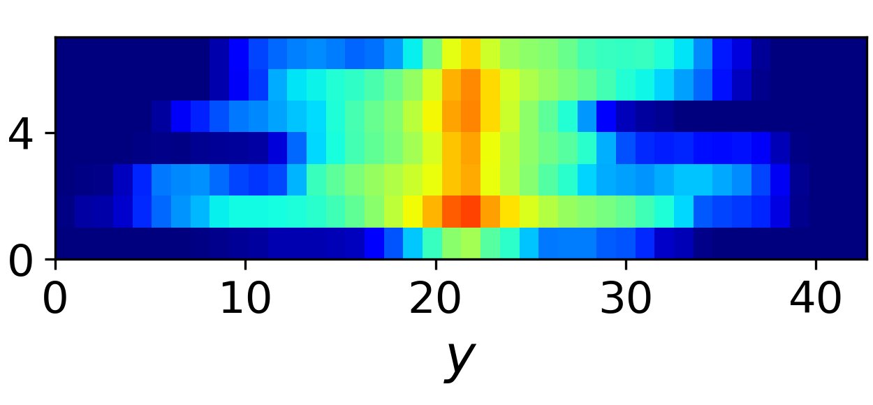
(b) Posterior 2 ($y$-$z$, sim)

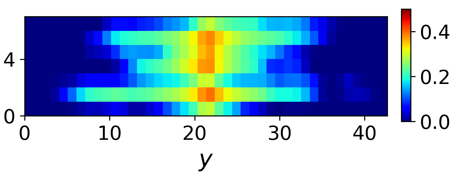
(c) Posterior 3 ($y$-$z$, sim)

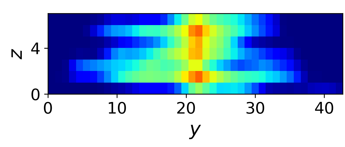
(d) Posterior 1 ($y$-$z$, surr)

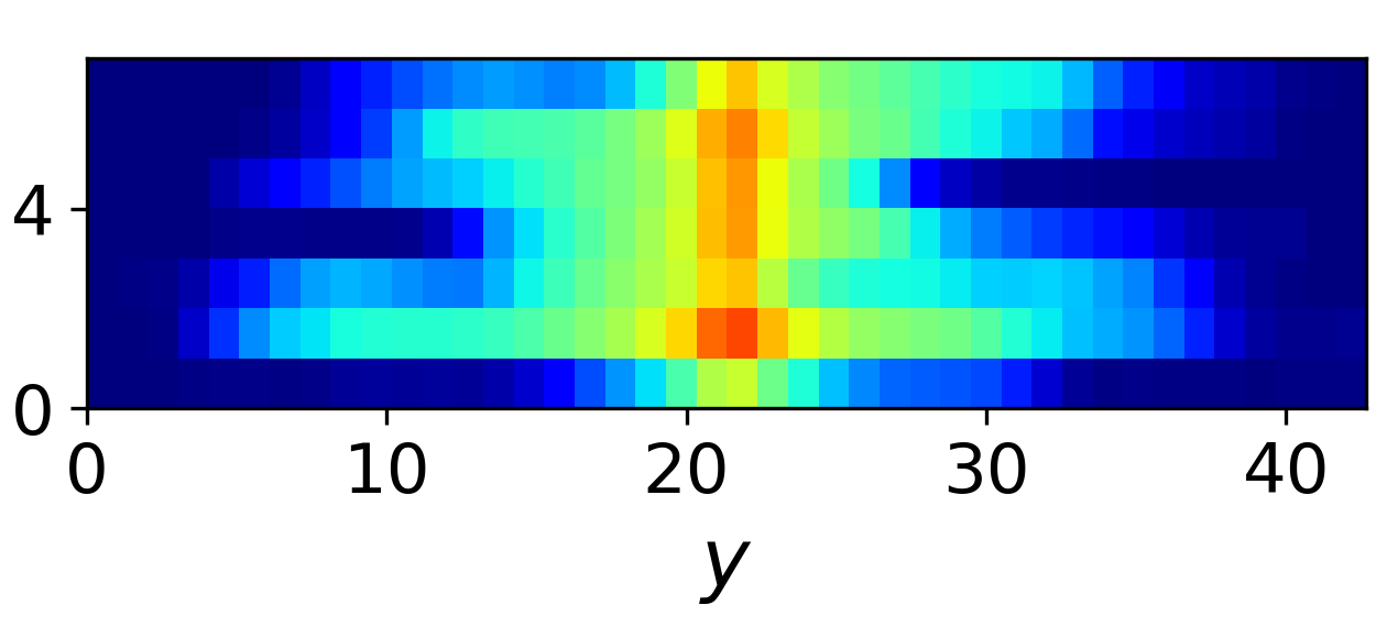
(e) Posterior 2 ($y$-$z$, surr)

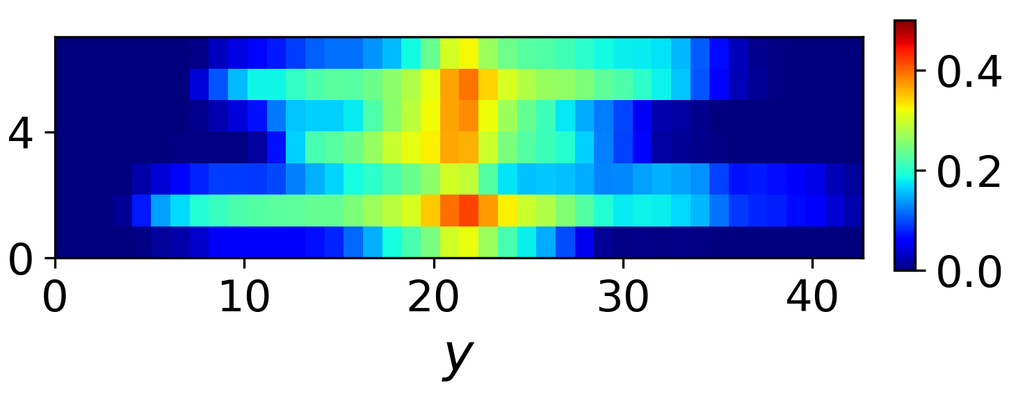
(f) Posterior 3 ($y$-$z$, surr)

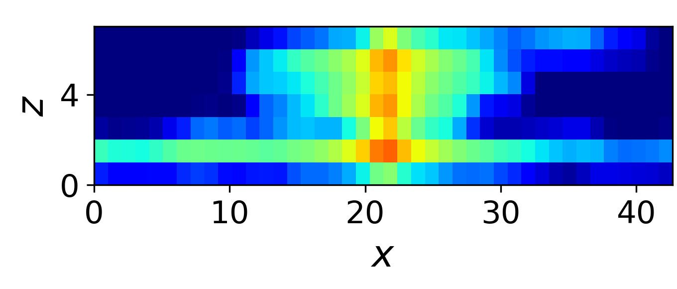
(g) Posterior 1 ($x$-$z$, sim)

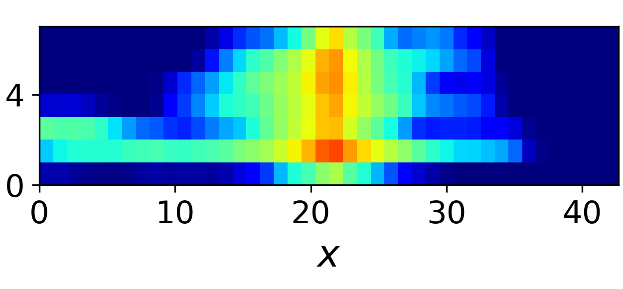
(h) Posterior 2 ($x$-$z$, sim)

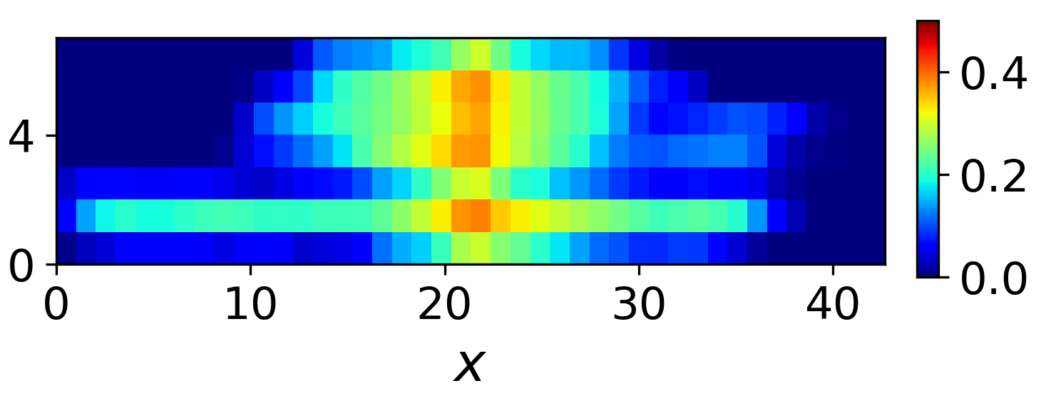
(i) Posterior 3 ($x$-$z$, sim)

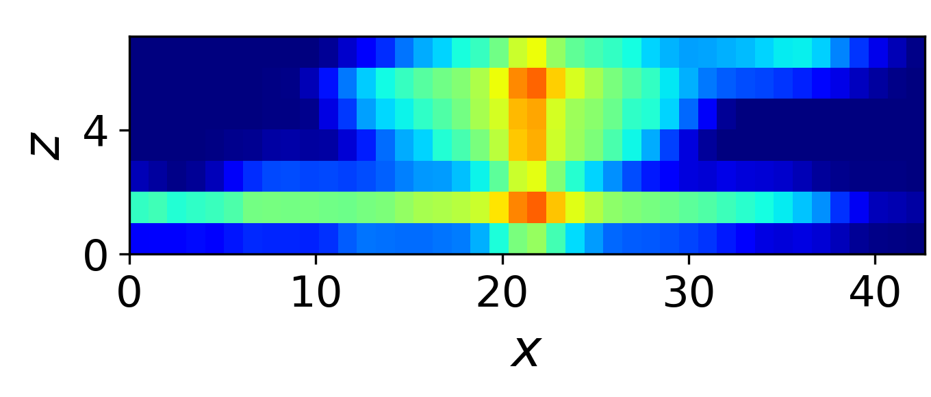
(j) Posterior 1 ($x$-$z$, surr)

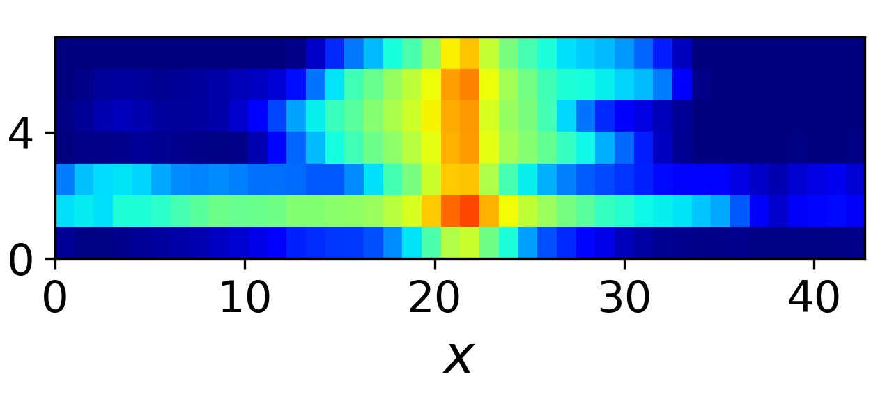
(k) Posterior 2 ($x$-$z$, surr)

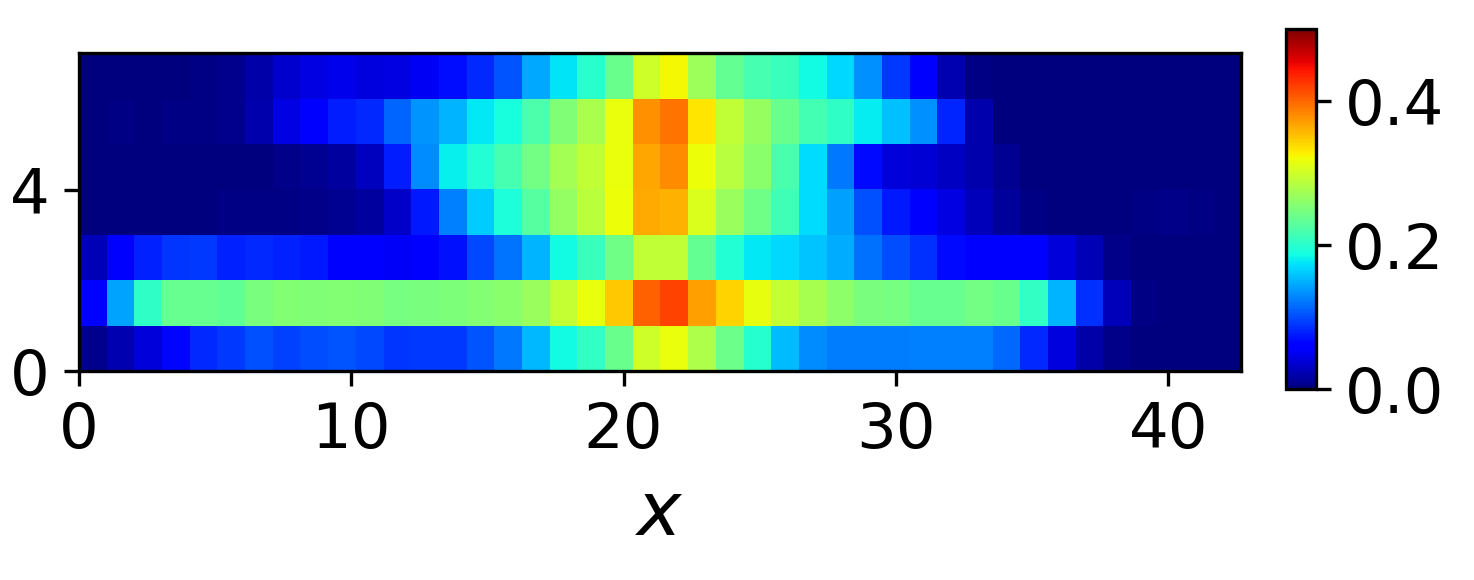
(l) Posterior 3 ($x$-$z$, surr)

Figure 18: Simulation and surrogate model results for saturation at 1 year for posterior realizations shown in Figure 17. Surrogate model results on row 2 correspond to simulation results on row 1, and surrogate model results on row 4 correspond to simulation results on row 3.

7 Concluding remarks

In this work, we implemented a deep-learning-based framework for history matching of geological carbon storage operations when both 4D seismic and monitoring well data are available. Our emphasis was on early time predictions, which are particularly important because uncertainty is high and unexpected behavior must be quickly identified. Two different fit-for-purpose deep learning surrogate models were constructed – one for predicting interpreted (coarse-scale) 4D seismic saturation fields, and one for predicting monitoring well data. Both networks accept high-resolution geomodels as input. The network for interpreted 4D seismic involves a 3D U-Net architecture, while the network for monitoring well data applies a 1D U-Net. Both networks have multiple output channels, with each channel corresponding to a different time step. The two specialized networks are simpler to construct and less time consuming to train than a single overall network able to provide global high-fidelity predictions.

The training samples for the two surrogate models were obtained by performing high-fidelity flow simulation, using the GEOS simulator, on 3500 geomodel realizations. These realizations were characterized by different geological scenario parameters (referred to as metaparameters), resulting in a high degree of variability. The interpreted seismic data used for training were constructed through application of a filtering procedure, which provides results at the scale informed by 4D seismic data. The performance of the surrogate models was evaluated on a test set of 500 new geomodels. Both surrogates were found to provide accurate predictions and both were shown to capture a variety of flow behaviors, as can occur given the high degree of prior uncertainty considered.

The deep learning surrogate models were then applied for data assimilation using a hierarchical MCMC method. History matching results were constructed using only monitoring well data and using both monitoring well and interpreted 4D seismic data. The impact of 4D seismic, in terms of reducing posterior uncertainty in the metaparameters over that achieved using only monitoring well data, was clearly demonstrated. Predictions for CO₂ plume shape and extent were also shown to be enhanced through inclusion of seismic data. A major advantage of our methodology is that the benefit of each data type can be quantified, and different strategies for combining highly-resolved local (monitoring well) data and coarse-resolution global (4D seismic) data can be quickly evaluated and thus optimized.

There are several topics that should be considered in future research. In this study, interpreted seismic saturation fields, assumed to be provided via petro-elastic inversion, were utilized. A higher degree of consistency would be achieved by working directly with seismic data rather than with interpreted data. In this case, the joint assimilation of both monitoring and seismic data could be addressed. Other data types, including pressure and surface displacement (which will require coupled flow-geomechanics simulations), are also expected to be informative and should be considered. Strategies for weighting and optimally combining these multiple data types, as well as error models, will also require investigation. Finally, the methodology developed here should be extended as necessary and then applied to practical storage operations.

References

- Aminu et al. (2017) Aminu, M.D., Nabavi, S.A., Rochelle, C.A., Manovic, V., 2017. A review of developments in carbon dioxide storage. Applied Energy 208, 1389–1419.
- Bui et al. (2021) Bui, Q.M., Hamon, F.P., Castelletto, N., Osei-Kuffuor, D., Settgast, R.R., White, J.A., 2021. Multigrid reduction preconditioning framework for coupled processes in porous and fractured media. Computer Methods in Applied Mechanics and Engineering 387, 114111.
- Bukshtynov et al. (2015) Bukshtynov, V., Volkov, O., Durlofsky, L.J., Aziz, K., 2015. Comprehensive framework for gradient-based optimization in closed-loop reservoir management. Computational Geosciences 19, 877–897.
- Chen et al. (2018) Chen, B., Harp, D.R., Lin, Y., Keating, E.H., Pawar, R.J., 2018. Geologic CO2 sequestration monitoring design: A machine learning and uncertainty quantification based approach. Applied Energy 225, 332–345.
- Chen et al. (2023) Chen, Z., Wang, M., Zhang, M., Huang, W., Gu, H., Xu, J., 2023. Post-processing refined ECG delineation based on 1D-UNet. Biomedical Signal Processing and Control 79, 104106.
- Çiçek et al. (2016) Çiçek, Ö., Abdulkadir, A., Lienkamp, S.S., Brox, T., Ronneberger, O., 2016. 3D U-Net: learning dense volumetric segmentation from sparse annotation, in: Medical Image Computing and Computer-Assisted Intervention–MICCAI 2016: 19th International Conference, Athens, Greece, October 17-21, 2016, Proceedings, Part II 19, Springer. pp. 424–432.
- Dadashpour et al. (2008) Dadashpour, M., Landrø, M., Kleppe, J., 2008. Nonlinear inversion for estimating reservoir parameters from time-lapse seismic data. Journal of Geophysics and Engineering 5, 54–66.
- Danaei et al. (2023) Danaei, S., Cirne, M., Maleki, M., Schiozer, D.J., Rocha, A., Davolio, A., 2023. All-in-one proxy to replace 4D seismic forward modeling with machine learning algorithms. Geoenergy Science and Engineering 222, 211460.
- Eigbe et al. (2023) Eigbe, P.A., Ajayi, O.O., Olakoyejo, O.T., Fadipe, O.L., Efe, S., Adelaja, A.O., 2023. A general review of CO2 sequestration in underground geological formations and assessment of depleted hydrocarbon reservoirs in the Niger Delta. Applied Energy 350, 121723.
- Emerick and Reynolds (2013) Emerick, A.A., Reynolds, A.C., 2013. Ensemble smoother with multiple data assimilation. Computers & Geosciences 55, 3–15.
- Evensen et al. (2007) Evensen, G., Hove, J., Meisingset, H.C., Reiso, E., Seim, K.S., Espelid, Ø., 2007. Using the EnKF for assisted history matching of a North Sea reservoir model, in: SPE Reservoir Simulation Conference, Society of Petroleum Engineers (SPE). pp. SPE–106184.
- Gelman et al. (1996) Gelman, A., Roberts, G.O., Gilks, W.R., 1996. Efficient Metropolis jumping rules, in: Bayesian Statistics 5: Proceedings of the Fifth Valencia International Meeting. Oxford University Press, pp. 599–608.
- Geng et al. (2017) Geng, C., MacBeth, C., Chassagne, R., 2017. Seismic history matching using a fast-track simulator to seismic proxy, in: SPE Europec featured at EAGE Conference and Exhibition, Society of Petroleum Engineers (SPE). p. D041S012R004.
- Gervais and Roggero (2010) Gervais, V., Roggero, F., 2010. Integration of saturation data in a history matching process based on adaptive local parameterization. Journal of Petroleum Science and Engineering 73, 86–98.
- Han et al. (2024) Han, Y., Hamon, F.P., Jiang, S., Durlofsky, L.J., 2024. Surrogate model for geological CO2 storage and its use in hierarchical MCMC history matching. Advances in Water Resources 187, 104678.
- Hastings (1970) Hastings, W.K., 1970. Monte Carlo sampling methods using Markov chains and their applications. Biometrika 57, 97–109.
- Hou et al. (2021) Hou, X., Wang, X., Hu, Y., Chen, Y., Huang, G., Nie, S., 2021. A one-dimensional U-Net-based calibration-transfer method for low-field nuclear magnetic resonance signals. Analytical Chemistry 93, 10469–10476.
- Kingma and Ba (2014) Kingma, D.P., Ba, J., 2014. Adam: A method for stochastic optimization. arXiv preprint arXiv:1412.6980 .
- Krevor et al. (2012) Krevor, S.C., Pini, R., Zuo, L., Benson, S.M., 2012. Relative permeability and trapping of CO2 and water in sandstone rocks at reservoir conditions. Water Resources Research 48, W02532.
- Li (2012) Li, Y., 2012. MOMCMC: An efficient monte carlo method for multi-objective sampling over real parameter space. Computers & Mathematics with Applications 64, 3542–3556.
- Liu et al. (2019) Liu, L., Jiang, H., He, P., Chen, W., Liu, X., Gao, J., Han, J., 2019. On the variance of the adaptive learning rate and beyond. arXiv preprint arXiv:1908.03265 .
- Lorentzen et al. (2024) Lorentzen, R.J., Bhakta, T., Fossum, K., Haugen, J.A., Lie, E.O., Ndingwan, A.O., Straith, K.R., 2024. Ensemble-based history matching of the Edvard Grieg field using 4D seismic data. Computational Geosciences 28, 129–156.
- Lumley (2010) Lumley, D., 2010. 4D seismic monitoring of CO2 sequestration. The Leading Edge 29, 150–155.
- MacBeth et al. (2016) MacBeth, C., Geng, C., Chassagne, R., 2016. A fast-track simulator to seismic proxy for quantitative 4D seismic analysis, in: SEG Technical Program Expanded Abstracts 2016. Society of Exploration Geophysicists, pp. 5537–5541.
- Mo et al. (2019) Mo, S., Zabaras, N., Shi, X., Wu, J., 2019. Deep autoregressive neural networks for high-dimensional inverse problems in groundwater contaminant source identification. Water Resources Research 55, 3856–3881.
- Nicolaidou et al. (2022) Nicolaidou, E., Birchwood, R., Prioul, R., Rodriguez-Herrera, A., 2022. Stochastic inversion of wellbore stability models calibrated with hard and soft data, in: ARMA US Rock Mechanics/Geomechanics Symposium, ARMA. pp. ARMA–2022.
- Oliver et al. (2021) Oliver, D.S., Fossum, K., Bhakta, T., Sandø, I., Nævdal, G., Lorentzen, R.J., 2021. 4D seismic history matching. Journal of Petroleum Science and Engineering 207, 109119.
- Oliver et al. (2008) Oliver, D.S., Reynolds, A.C., Liu, N., 2008. Inverse theory for petroleum reservoir characterization and history matching. Cambridge University Press.
- Padhi et al. (2014) Padhi, A., Mallick, S., Behzadi, H., Alvarado, V., 2014. Efficient modeling of seismic signature of patchy saturation for time lapse monitoring of carbon sequestrated deep saline reservoirs. Applied Energy 114, 445–455.
- Rana et al. (2018) Rana, S., Ertekin, T., King, G.R., 2018. An efficient probabilistic assisted history matching tool using Gaussian processes proxy models: application to coalbed methane reservoir, in: SPE Annual Technical Conference and Exhibition, Society of Petroleum Engineers (SPE). p. D021S014R001.
- Remy et al. (2009) Remy, N., Boucher, A., Wu, J., 2009. Applied geostatistics with SGeMS: A user’s guide. Cambridge University Press.
- Ronneberger et al. (2015) Ronneberger, O., Fischer, P., Brox, T., 2015. U-Net: Convolutional networks for biomedical image segmentation, in: Medical image computing and computer-assisted intervention–MICCAI 2015: 18th international conference, Munich, Germany, October 5-9, 2015, proceedings, part III 18, Springer. pp. 234–241.
- Rossi Rosa et al. (2023) Rossi Rosa, D., Schiozer, D.J., Davolio, A., 2023. Data assimilation of production and multiple 4D seismic acquisitions in a deepwater field using ensemble smoother with multiple data assimilation. SPE Reservoir Evaluation & Engineering 26, 1528–1540.
- Rwechungura et al. (2011) Rwechungura, R., Dadashpour, M., Kleppe, J., 2011. Advanced history matching techniques reviewed, in: SPE Middle East Oil and Gas Show and Conference, Society of Petroleum Engineers (SPE). pp. SPE–142497.
- Souza et al. (2019) Souza, R., Lumley, D., Shragge, J., Davolio, A., Schiozer, D., 2019. 4D seismic bandwidth and resolution analysis for reservoir fluid flow model applications. ASEG Extended Abstracts 2019, 1–5.
- Sun and Durlofsky (2019) Sun, W., Durlofsky, L.J., 2019. Data-space approaches for uncertainty quantification of CO2 plume location in geological carbon storage. Advances in Water Resources 123, 234–255.
- Tang and Durlofsky (2024) Tang, H., Durlofsky, L.J., 2024. Graph network surrogate model for subsurface flow optimization. Journal of Computational Physics 512, 113132.
- Tang et al. (2020) Tang, M., Liu, Y., Durlofsky, L.J., 2020. A deep-learning-based surrogate model for data assimilation in dynamic subsurface flow problems. Journal of Computational Physics 413, 109456.
- Tiwari et al. (2021) Tiwari, P.K., Das, D.P., Patil, P.A., Chidambaram, P., Chandran, P.K., Tewari, R.D., Abdul Hamid, M.K., 2021. 4D seismic in subsurface CO2 plume monitoring–why it matters?, in: SPE Annual Technical Conference and Exhibition, Society of Petroleum Engineers (SPE). p. D021S033R006.
- Wang et al. (2021) Wang, N., Chang, H., Zhang, D., 2021. Deep-learning-based inverse modeling approaches: A subsurface flow example. Journal of Geophysical Research: Solid Earth 126, e2020JB020549.
- Wang et al. (2022) Wang, N., Chang, H., Zhang, D., 2022. Surrogate and inverse modeling for two-phase flow in porous media via theory-guided convolutional neural network. Journal of Computational Physics 466, 111419.
- Wen et al. (2023) Wen, G., Li, Z., Long, Q., Azizzadenesheli, K., Anandkumar, A., Benson, S.M., 2023. Real-time high-resolution CO2 geological storage prediction using nested Fourier neural operators. Energy & Environmental Science 16, 1732–1741.
- Zhang et al. (2023) Zhang, Z., He, X., AlSinan, M., Kwak, H., Hoteit, H., 2023. Robust method for reservoir simulation history matching using Bayesian inversion and long-short-term memory network-based proxy. SPE Journal 28, 983–1007.