Embodiment: Self-Supervised Depth Estimation Based on Camera Models

Abstract

Depth estimationn is a critical topic for robotics and vision-related tasks. In monocular depth estimation, in comparison with supervised learning that requires expensive ground truth labeling, self-supervised methods possess great potential due to no labeling cost. However, self-supervised learning still has a large gap with supervised learning in 3D reconstruction and depth estimation performance. Meanwhile, scaling is also a major issue for monocular unsupervised depth estimation, which commonly still needs ground truth scale from GPS, LiDAR, or existing maps to correct. In the era of deep learning, existing methods primarily rely on exploring image relationships to train unsupervised neural networks, while the physical properties of the camera itself—such as intrinsics and extrinsics—are often overlooked. These physical properties are not just mathematical parameters; they are embodiments of the camera’s interaction with the physical world. By embedding these physical properties into the deep learning model, we can calculate depth priors for ground regions and regions connected to the ground based on physical principles, providing free supervision signals without the need for additional sensors. This approach is not only easy to implement but also enhances the effects of all unsupervised methods by embedding the camera’s physical properties into the model, thereby achieving an embodied understanding of the real world.

I INTRODUCTION

Monocular depth estimation serves as a cornerstone in robotics [14], 3D mapping [20], camera localization [24, 23], and augmented reality [29]. This process aims to derive depth from a single RGB image, an inherently challenging task due to scale ambiguity, where one 2D image might represent numerous possible 3D scenes. Convolutional neural networks have significantly advanced this area [15], though most cutting-edge methods rely on supervised training [6, 2], necessitating sparse depth ground truth from instruments like LiDAR. The high cost and labor of data collection and labeling constrain the data scale for supervised approaches [2]. To avoid the need for depth labeling, there has been a shift towards self-supervised frameworks, employing regression modules for pixel-wise depth estimation and photometric consistency loss for model training [12]. Despite these efforts, self-supervised learning for monocular depth estimation still faces significant accuracy challenges, often misestimating objects’ 3D structures as either too distant or too close due to the indirect nature of photometric and cross-frame consistency constraints.

Meanwhile, due to the convenience brought by deep neural networks, extensive information from the sensors themselves has been ignored. This paper introduces a method that leverages camera model parameters (both intrinsic and extrinsic) to accurately calculate depth information, thereby embedding the camera model and its physical characteristics into the deep learning model. This approach goes beyond mere mathematical computation; it embodies the interaction between the camera and the physical world. By integrating these physical characteristics into the deep learning model, we can accurately determine the depth for much of the scene, facilitating neural network training without the need for explicit ground truth data. The method also incorporates image semantics to calculate the ground plane’s depth, allowing for the estimation of the depth of objects on the ground, such as buildings and vehicles. Utilizing this physics-based supervision approach, the framework not only enhances the performance of unsupervised networks but also achieves an embodied understanding of the real world, providing strong support for detailed 3D structure modeling. Importantly, our algorithm serves as a valuable extension for any unsupervised depth estimation effort.

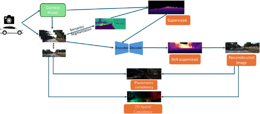
Figure 1: The framework for unsupervised 3D scene reconstruction neural network based on physics depth calculated from camera models. We first calculate the physical depth of flat ground areas in the input image using the camera model and semantic segmentation results. This physical depth serves as a label for supervised learning, providing a foundation for initial depth estimation. In the first stage, we train the depth estimation network with these labels. In the subsequent self-supervised stage, we introduce photometric and 2D spatial losses, which optimize depth estimation based on image characteristics without relying on depth labels.

In summary, our main contributions include the following aspects: 1. We propose a novel mechanism that leverages the physical model parameters of the camera to calculate the depth information for a large portion of the scene, embedding the camera model and its physical properties into the deep learning model to supervise the depth estimation network. We refer to this depth information, derived from the camera’s physical model, as physics depth. 2. To address the uncertain scale issue in unsupervised monocular depth estimation, our approach provides an absolute scale instead of just a relative scale. 3. We designed a neural network training framework to effectively integrate physics depth supervision with unsupervised methods, specifically targeting the physics depth calculated from the camera model. The framework for physics depth computation and training with the self-supervised network is shown in Fig. 1.

II Relate Work

II-A Self-Supervised Depth Estimation

Self-supervised depth estimation from monocular videos or stereo image pairs is gaining prominence, particularly due to the challenges in obtaining accurate ground truth. [38] spearheaded a self-supervised framework by jointly training depth and pose networks based on image reconstruction loss. [12] further advanced this field by introducing a minimum reprojection loss and auto-masking loss, setting a new benchmark. [13] and [4] integrated real-time data sources such as GPS or camera velocity to address the scale ambiguity inherent in monocular Structure-from-Motion (SfM) methods. These self-supervised models hinge on the photometric consistency of the reprojection. In stereo training contexts, models use synchronous stereo image pairs to predict disparity [28], which inversely relates to depth. Since the relative camera pose is known in stereo setups, the primary task of these models is disparity prediction. [9] pioneered this approach, training a self-supervised monodepth model using stereo pairs and a photometric consistency loss. This methodology was further refined by [11] with additional constraints like left-right consistency and bundle adjusted pose graph [22]. Moreover, [8] extended it to predict continuous disparity. Stereo views naturally offer an absolute depth scale, whereas current monocular self-supervised models only predict relative depths, needing ground truth for scale calibration. Utilizing physics depth data from ground surfaces and road-connecting areas can improve these unsupervised models to predict absolute depths, enhancing accuracy for datasets such as KITTI.

II-B Geometric Priors

Geometric priors are becoming crucial for monocular depth estimation, evolving beyond the optimization-focused traditional multi-view stereo methods noted by [7]. In self-supervised learning, multi-view geometry is essential, enabling image warping from source to target viewpoints to generate reprojection errors. These errors act as the loss function for depth estimation networks [12]. Moreover, geometric consistency, especially in comparing point clouds, is gaining attention as a valuable complement to photometric consistency [26]. The surface normal constraint, highlighted in works by [17] and [21], is a key geometric prior ensuring the alignment of normal vectors from both estimated and actual depth data. However, this approach can lead to inaccuracies in depth estimations, especially in areas with high curvature, underscoring the limitations of relying solely on planarity assumptions.

III Embodiment Physics Depth

III-A Physics depth for Full Field of view

We introduce a novel monocular depth estimation technique called ”physics depth”. This method leverages the camera’s intrinsic and extrinsic parameters, as well as semantic segmentation, to calculate absolute depth, embedding the physical characteristics of the camera model into the deep learning model. This approach derives depth from basic physical principles, assuming the camera captures initially flat surfaces. We refine depth estimates by identifying truly flat areas through semantic segmentation, extending depth to adjacent areas, and filling gaps with inpainting. Our method, tested on KITTI, CityScape, and Make3D datasets, achieves accuracy comparable to LiDAR, especially for close, flat surfaces. Our model is based on the pinhole camera model, which is widely used in practical applications due to its minimal distortion, making it an ideal reference point for achieving embodiment. Although designed with the pinhole model in mind, our method can be adapted for different camera types by adjusting for each camera’s unique characteristics. For every image pixel, we compute a unit vector $\hat{r}$ representing the camera ray’s direction in the physical world, translating pixel positions into directional vectors that indicate the camera’s viewpoint in real space.

$$\centering\vspace{-2mm}\begin{array}[]{l}\hat{r}=\frac{{\left[{u,v,f}\right]}}{{\sqrt{{u^{2}}+{v^{2}}+{f^{2}}}}}\end{array}\@add@centering$$ (1)

where ($u$, $v$) represents the coordinates of the pixel, with the origin of the coordinate system situated at the optical center (${{O_{x}},{O_{y}}}$) of the image, commonly referred to as the principal point. Meanwhile, $f=({{f_{x}}+{f_{y}}})/2$, where ${f_{x}}$ and ${f_{y}}$ denote the camera’s focal length in the $x$ and $y$ directions.

To generate a physics depth scaled to dimensions different from those of the original RGB image, the parameters of the unit vector $\hat{r}$ must be adjusted accordingly. Suppose $W_{\text{org}}$ and $H_{\text{org}}$ are the width and height of the original RGB image, and $W_{\text{new}}$ and $H_{\text{new}}$ are the desired width and height for the physics depth. Let $S_{\text{width}}$ and $S_{\text{height}}$ represent the scaling factors for the width and height, respectively, where $S_{\text{width}}=\frac{W_{\text{new}}}{W_{\text{org}}}$ and $S_{\text{height}}=\frac{H_{\text{new}}}{H_{\text{org}}}$. The scale-adjusted pixel coordinates ($u^{\prime},v^{\prime}$) are given by ($S_{\text{width}}\times u,S_{\text{height}}\times v$). The scale-adjusted optical center coordinates ($O_{x}^{\prime},O_{y}^{\prime}$) are ($S_{\text{width}}\times O_{x},S_{\text{height}}\times O_{y}$), and the scale-adjusted focal lengths ($f_{x}^{\prime},f_{y}^{\prime}$) are ($S_{\text{width}}\times f_{x},S_{\text{height}}\times f_{y}$), as determined by perspective projection. The scale-adjusted unit vector $\hat{r^{\prime}}$ can be derived using the below equation by updating the parameters in Eq. 1:

$$R_{roll} =\left[\begin{array}[]{ccc}1&0&0\\ 0&\cos(\text{roll})&\sin(\text{roll})\\ 0&-\sin(\text{roll})&\cos(\text{roll})\end{array}\right],$$ (2)

$$R_{pitch} =\left[\begin{array}[]{ccc}\cos(\text{pitch})&0&-\sin(\text{pitch})\\ 0&1&0\\ \sin(\text{pitch})&0&\cos(\text{pitch})\end{array}\right],$$

$$R_{yaw} =\left[\begin{array}[]{ccc}\cos(\text{yaw})&\sin(\text{yaw})&0\\ -\sin(\text{yaw})&\cos(\text{yaw})&0\\ 0&0&1\end{array}\right]$$

$$\centering\begin{array}[]{l}{R_{c}}={R_{yaw}}*{R_{pitch}}*{R_{roll}}\end{array}\vspace{-2mm}\@add@centering$$ (3)

Using $R_{c}$ we rotate the camera ray vector to align it with the ground coordinate system: $\hat{r_{c}}={R_{c}}*\hat{r^{\prime}}$

Since $\hat{r_{c}}({r_{c,u}},{r_{c,v}},{r_{c,f}})$ is a unit vector, the 3D coordinates of the point, $P=(x_{c},y_{c},z_{c})$, on the ground surface in camera’s coordinate system can be determined by multiplying $r_{c}$ with the point-to-point distance ($d$) of the ground point from camera.

$$\left[x_{c},y_{c}\right]=d*\left[{{r_{c,u}},{r_{c,v}}}\right]$$ (4)

When the height of the camera ($h$) is known from the camera’s extrinsic parameters and assuming the camera coordinate system’s y-axis is oriented downwards, then ${y_{c}}$ = $h$, and the point-to-point distance $d$ and ${x_{c}}$ can be calculated as shown:

$$d=\frac{h}{{{r_{c,v}}}},{x_{c}}=d*{r_{c,u}}\vspace{-2mm}$$ (5)

The projection of a three-dimensional point from the camera coordinate system $(x_{c},y_{c},z_{c})$ to the two-dimensional image plane $(u,v)$, can be accurately represented using the following linear camera model equation:

$${Z_{c}}\left[\begin{array}[]{c}u\\ v\\ 1\end{array}\right]=\left[\begin{array}[]{ccc}{{f_{x}^{\prime}}}&0&{{O_{x}^{\prime}}}\\ 0&{{f_{y}^{\prime}}}&{{O_{y}^{\prime}}}\\ 0&0&1\end{array}\right]\!\left[\begin{array}[]{c}{{x_{c}}}\\ {{y_{c}}}\\ {{z_{c}}}\\ \end{array}\right]$$ (6)

where $\mathbf{K}$ denotes the camera’s intrinsic matrix:

$${K}=\left[\begin{array}[]{ccc}{{f_{x}^{\prime}}}&0&{{O_{x}^{\prime}}}\\ 0&{{f_{y}^{\prime}}}&{{O_{y}^{\prime}}}\\ 0&0&1\end{array}\right]$$ (7)

By substituting $x_{c}$, $y_{c}$ in Eq. 6, we derive $z_{c}$ for a given pixel $(u,v)$ that maps to a ground point. This process allows calculating depth and 3D coordinates in the camera coordinate system for ground surface pixels, given the camera’s height. We tested our approach on the KITTI [10] and Cityscapes [5] datasets, with results detailed in Section V-B.

Our method improves depth estimation by closely aligning it with LiDAR data on flat surfaces like roads, providing more detail than standard sparse LiDAR data, as demonstrated on the KITTI and Cityscapes datasets. Initially targeting flat surfaces may risk overfitting, limiting versatility. To counter this, we expanded our physics depth approach to cover the entire image, including vertical structures like cars and buildings. This involves deriving depth by extending upwards from where flat and vertical surfaces meet, creating a comprehensive ground physics depth as detailed in Section V-B. We extended physics depth to vertical objects in contact with flat surfaces, such as vehicles, pedestrians, and buildings, by propagating depth values upward from their points of intersection with the ground, termed as Edge Extended Physics Depth. We assume these vertical entities have a consistent depth with the ground they touch, enabling us to infer their depth directly from the ground. This approach greatly improves the accuracy and consistency of depth estimation throughout the image. After vertically extending physics depth, we encountered objects with incomplete depth due to their limited contact with the ground. We used the Telea Inpainting Technique [30] to fill these gaps, leveraging its fast and effective method based on the surrounding pixels’ directional changes and geometric distances. For objects not touching the ground, we projected depth from nearby objects to ensure continuity. Additionally, we assigned the sky a depth 1.5 times the maximum of the inpainted depths, achieving a gap-free Dense Physics Depth. This approach primarily serves to create an improved depth prior, enhancing overall depth estimation accuracy.

The effectiveness of our method has been validated using the KITTI [10] and Cityscapes [5] datasets, with results showing a close alignment in accuracy with LiDAR-derived depth measurements, especially for proximal flat surfaces.

IV Interaction Between Physics-Depth Supervision and Self-Supervision

IV-A Network Architecture

Our research addresses the data scarcity in physics depth, which is typically limited to only portions of an image and, by itself, inadequate for self-supervised learning. By embedding the physical characteristics of the camera model into the deep learning model, we utilize physics depth as an embodied prior, enhancing depth estimation. Unlike traditional self-supervised models that typically start with random depth values, our model can more accurately refine the depth estimation of ground surfaces and surrounding areas. This approach significantly improves efficiency in correcting depth inaccuracies through self-supervised training. Our model uniquely combines RGB and physics depth, adding valuable depth insights. During the supervised phase, we assess the confidence in physics depth to focus learning on the reliable areas. For self-supervised learning, we advance the model by integrating geometric consistency with photometric consistency, leading to more precise depth estimates.

IV-B Physics-Depth Supervision

In this study, we calculate the physical depth of ground areas in each image using the camera model and employ it as an initial guide during the depth network training phase to enhance the model’s understanding of depth across various regions. These physical depth data serve as labels for supervised learning, significantly improving the model’s comprehension and prediction of ground area depths. Specifically, we first utilize the camera’s intrinsic and extrinsic parameters, along with the semantic segmentation results of the images, to accurately calculate the physical depth of ground areas. These physical depth data provide initial guidance to the model, equipping it with a fundamental understanding of spatial depth. This not only ensures the model has reliable depth information at the initial training stage but also effectively reduces dependence on randomly initialized depths, thereby preventing substantial error propagation during early training. During training, the physical depth data act as supervisory signals, enabling the model to better learn the geometric structure of ground areas. This approach allows the model to more accurately capture the actual depth information of the ground and extend this understanding to the entire scene. The reliability of physical depth ensures the model performs more robustly and accurately when handling areas with similar geometric characteristics. Furthermore, physical depth serves as a benchmark, helping the model better correct prediction errors. In subsequent training stages, by integrating physical depth with other self-supervised signals (such as photometric and geometric consistency), the model can further optimize depth prediction results. Ultimately, the foundational knowledge provided by physical depth significantly enhances the model’s depth prediction accuracy and robustness, leading to excellent performance in practical applications.

$$\centering\begin{array}[]{l}{L_{phy}}=\sum\nolimits_{i=1}^{M}{\sum\nolimits_{j=1}^{N}{{{\left({d_{ij}^{phy}-{{\hat{d}}_{ij}}}\right)}^{2}}}}\end{array}\vspace{-2mm}\@add@centering$$ (8)

$d_{ij}^{phy}$ is the physics depth of $\left({i,j}\right)$ as a label for supervision pixel point as a label for supervised learning. ${\hat{d}_{ij}}$ is the depth of $\left({i,j}\right)$ predicted by the model.

Our model uses physics depth as its starting point, which helps in accurately predicting real depth. This is important because estimating depth from a single camera view often leads to scale issues, where the same point can appear to have different depths. Most single-view models can only estimate depth relative to other points, not the actual depth. However, our method uses physics depth during training, enabling the model to learn and correct errors in depth prediction. Since physics depth represents the true depth, it maintains scale accuracy during these corrections. Thus, our model effectively overcomes the scale problem in single depth estimation.

IV-C Self-Supervised Training

In the self-supervised training paradigm, depth estimation is framed as an image reconstruction problem. This approach avoids the need for ground truth labels by utilizing unlabeled monocular videos during training. Our methodology leverages both photometric and geometric consistencies as dual pillars to jointly optimize image reconstruction.

IV-C1 Photometric Consistency

For consecutive frames $I_{t-1}$ and $I_{t}$, our model independently estimates their corresponding depths, $D_{t-1}$ and $D_{t}$. As outlined in Eq. 9, frames $I_{t-1}$ and $I_{t}$ can be projected into structured 3D point clouds $Q_{t-1}$ and $Q_{t}$, respectively. Utilizing the pose network, we estimate the camera’s motion from time $t-1$ to $t$. Through the application of the transformation matrix $T_{t-1\to t}$ and the point cloud $Q_{t}$, an estimated version of $Q_{t-1}$, denoted as ${\hat{Q}}_{t-1}$, is obtained as ${\hat{Q}}_{t-1}=T_{t-1\to t}Q_{t}$. Subsequently, frame $I_{t}$ is reconstructed by warping $I_{t-1}$ using the principles detailed in Eq. 10. The photometric loss is computed by Eq. 10 using reconstructed target image ${{I_{t-1\to t}}}$ and target image ${{I_{t}}}$.

$$\centering\begin{array}[]{l}Q_{t-1}^{xy}=D_{t-1}^{xy}\cdot{K^{-1}}\left[{\begin{array}[]{*{20}{c}}x\\ y\\ 1\end{array}}\right]\end{array}\@add@centering$$ (9)

$$\centering\begin{array}[]{l}{I_{t-1\to t}}\left[u\right]={I_{t-1}\left\langle{u^{\prime}}\right\rangle},{L_{ph}}=ph\left({{I_{t}},{I_{t-1\to t}}}\right)\vspace{-3mm}\end{array}\@add@centering$$ (10)

$$\begin{array}[]{l}ph\left({{I_{t}},{I_{t-1\to t}}}\right)=\frac{\alpha}{2}\left({1-SSIM\left({{I_{t}},{I_{t-1\to t}}}\right)}\right)\\ +\left({1-\alpha}\right){\left\|{\left({{I_{t}},{I_{t-1\to t}}}\right)}\right\|_{1}}\end{array}$$ (11)

Here $\alpha$ is commonly set to 0.85 [12], ph is a photometric reconstruction error. Furthermore, for each pixel p, the minimum of the losses computed from forward and backward neighboring frames allows the mitigation of the effect of occlusions [12] on the reprojection process.

$$\centering\begin{array}[]{l}{L_{ph}}\left(p\right)=\mathop{\min}\limits_{s\in\left[{-1,1}\right]}pe\left({{I_{t-1}}\left(p\right),{I_{{t-1}\to t}}\left(p\right)}\right)\end{array}\@add@centering$$ (12)

$1$ stands for forward, $-1$ stands for backward.

Method	Scale	Test	AbsRel ↓	Sq Rel↓	RMSE↓	RMSElog ↓	$\delta<1.25$ ↑	$\delta<1.25^{2}$ ↑	$\delta<1.25^{3}$ ↑
Monodepth2 [12]	LiDAR Scale	32.260	0.159	1.689	5.168	0.238	0.830	0.931	0.967
	Physics Depth Scale	32.487	0.158	1.968	5.287	0.242	0.842	0.930	0.966
MonoVit [37]	LiDAR Scale	28.354	0.110	0.759	4.248	0.199	0.872	0.954	0.979
	Physics Depth Scale	28.096	0.108	0.743	4.241	0.200	0.874	0.955	0.979
SQLDepth [33]	LiDAR Scale	43.51	0.087	0.659	4.096	0.165	0.920	0.970	0.984
	Physics Depth Scale	44.17	0.089	0.664	4.101	0.169	0.918	0.969	0.982

TABLE I: Evaluation of different models with LiDAR Depth Scaling Factor and Physics Depth Scaling Factor.

KITTI Date	Road Physics Depth Error: +/- 5%	Road Physics Depth Error: +/- 10%	Flat Surface Physics Depth Error: +/- 5%	Flat Surface Physics Depth Error: +/- 10%
2011-09-26	84.28%	96.26%	75.08%	89%
2011-09-28	80.61%	85.64%	61.21%	77%
2011-09-29	90.53%	97.34%	74.46%	91%
2011-09-30	76.43%	91.86%	56.98%	81%
2011-10-0	78.12%	94.61%	62.77%	85%

TABLE II: Error between physics depth and KITTI ground truth. The proportion of the 5-days road physics depth error and the flat surface physics depth error within $5\%$ and within $10\%$ of ground truth, respectively, in the KITTI dataset.

City	Road Physics Depth Error: +/- 5%	Road Physics Depth Error: +/- 10%	Flat Surface Physics Depth Error: +/- 5%	Flat Surface Physics Depth Error: +/- 10%
aachen	87.48%	94.77%	73.17%	86.94%
bochum	80.76%	93.22%	65.51%	83.95%
bremen	86.55%	97.64%	72.60%	88.29%
cologne	81.66%	98.88%	75.14%	88.82%
darmstadt	82.49%	95.44%	69.95%	86.56%
dusseldorf	83.22%	93.59%	68.79%	84.96%
erfurt	83.78%	94.26%	69.58%	85.85%
hamburg	82.77%	96.81%	67.93%	84.22%
hanover	76.59%	97.45%	64.71%	83.00%
monchengladbach	83.42%	94.73%	63.75%	82.48%
strasbourg	84.63%	95.62%	61.44%	81.52%
stuttgart	80.49%	96.38%	68.52%	85.26%
tubingen	85.44%	92.76%	67.22%	84.69%
ulm	89.00%	98.38%	73.35%	87.89%
weimar	80.06%	93.69%	64.47%	82.58%
zurich	88.99%	97.52%	70.72%	85.82%
jena	77.90%	92.85%	63.75%	81.85%
krefeld	86.23%	94.11%	65.83%	83.92%

TABLE III: Error between physics depth and Cityscape ground truth: The proportion of Road Physics Depth Error and Flat Surface Physics Depth Error for different cities in the cisyscape dataset.

	Road Physics Depth	Ground PhysicsDepth
+/- 5% error	80.24%	60.30%
+/- 10% error	99.33%	74.89%

TABLE IV: Physics depth in a sample KITTI image.

Method	Type	Year	Resolution	AbsRel ↓	Sq Rel↓	RMSE↓	RMSE log↓	$\delta<1.25$ ↑	$\delta<1.25^{2}$ ↑	$\delta<1.25^{3}$ ↑
Monodepth2 [12]	MS	2019	1024×320	0.106	0.806	4.630	0.193	0.876	0.958	0.980
HR-Depth [25]	MS	2021	1024×320	0.101	0.716	4.395	0.179	0.899	0.966	0.983
Lite-Mono [36]	M	2023	1024×320	0.097	0.710	4.309	0.174	0.905	0.967	0.984
MonoVIT [37]	M	2023	1024×320	0.096	0.714	4.292	0.172	0.908	0.968	0.984
DualRefine [1]	MS	2023	1024×320	0.096	0.694	4.264	0.173	0.908	0.968	0.984
ManyDepth [34]	M	2021	1024×320	0.087	0.685	4.142	0.167	0.920	0.968	0.983
RA-Depth [16]	M	2022	1024×320	0.097	0.608	4.131	0.174	0.901	0.968	0.985
PlaneDepth [32]	MS	2023	1280×384	0.090	0.584	4.130	0.182	0.896	0.962	0.981
SQLDepth [33]	M	2023	1024×320	0.087	0.659	4.096	0.165	0.920	0.970	0.984
Ours (Backbone: SQLDepth)	M	2023	1024×320	0.085	0.583	3.885	0.158	0.922	0.970	0.986

TABLE V: The quantitative depth comparison using the Eigen split of the KITTI dataset  [10]. M: trained with monocular videos; MS: trained with stereo pairs.

Method	Size	Test	AbsRel ↓	Sq Rel↓	RMSE↓	RMSElog ↓	$\delta<1.25$ ↑	$\delta<1.25^{2}$ ↑	$\delta<1.25^{3}$ ↑
Pilzer et al [27]	$512\times\ 256$	1	0.240	4.264	8.049	0.334	0.710	0.871	0.937
Struct2Depth [3]	$416\times\ 128$	1	0.145	1.737	7.280	0.205	0.813	0.942	0.976
Monodepth2 [12]	$416\times\ 128$	1	0.129	1.569	6.876	0.187	0.849	0.957	0.983
Lee [19]	$832\times\ 256$	1	0.111	1.158	6.437	0.182	0.868	0.961	0.983
InstaDM [18]	$832\times\ 256$	1	0.111	1.158	6.437	0.182	0.868	0.961	0.983
ManyDepth [34]	$416\times\ 128$	2	0.114	1.193	6.223	0.170	0.875	0.967	0.989
SQLDepth [33]	$416\times\ 128$	1	0.110	1.130	6.264	0.165	0.881	0.971	0.991
Ours (Backbone: SQLDepth)	$416\times\ 128$	1	0.103	1.090	6.237	0.157	0.895	0.974	0.991

TABLE VI: The quantitative depth comparison of the Cityscape dataset.

IV-C2 2D Spatial Consistency

Our method prioritizes spatial disparities to gauge scene geometry, which is key for decoding object interactions. This strategy excels in depth and scale depiction, functioning well in scenes with sparse texture or color and remaining stable against lighting or color shifts. We devised a model that refines pose and depth networks via a loss function, using spatial disparities to boost pose accuracy and depth perception. By utilizing dense optical flow, the model aligns points across frames to compute their movement, aiding in precise motion analysis. Our loss function, ${L_{2D}}$, is based on motion variance between actual and reconstructed frames, ${I_{t}}$ and ${\hat{I}_{t}}$, enhancing model accuracy.

$${L_{2D}}=\sum_{i=1}^{N}\left(\alpha\|\mathbf{v}_{t+1}^{(i)}-\mathbf{v}_{t}^{(i)}\|^{2}+\beta(1-\cos(\theta^{(i)}))\right)$$ (13)

$N$ represents the total number of matching points. $alpha$ and $beta$ are weight coefficients balancing the positional and directional differences. ${v}_{t}^{(i)}$ and $\mathbf{v}_{t+1}^{(i)}$ denote the motion vectors of the $i-th$ matching point in frames $t$ and $t+1$, respectively. $\theta^{(i)}$ is the angle between vectors $\mathbf{v}_{t}^{(i)}$ and $\mathbf{v}_{t+1}^{(i)}$, with $\cos(\theta^{(i)})=\frac{\mathbf{v}_{t}^{(i)}\cdot\mathbf{v}_{t+1}^{(i)}}{\|\mathbf{v}_{t}^{(i)}\|\|\mathbf{v}_{t+1}^{(i)}\|}$ representing the cosine of this angle. The first term in the loss function, $\|\mathbf{v}_{t+1}^{(i)}-\mathbf{v}_{t}^{(i)}\|^{2}$, quantifies the positional difference, whereas the second term, $1-\cos(\theta^{(i)})$, assesses the directional difference. The directional consistency is measured by the cosine of the angle between the motion vectors, where a value close to 1 indicates minimal directional change, and a value further from 1 signifies a greater change.

Method	Type	AbsRel ↓	Sq Rel↓	RMSE↓	log10↓
Zhou [38]	S	0.383	5.321	10.470	0.478
DDVO [31]	M	0.387	4.720	8.090	0.204
Monodepth2 [12]	M	0.322	3.589	7.417	0.163
CADepthNet [35]	M	0.312	3.086	7.066	0.159
SQLDepth [33]	M	0.306	2.402	6.856	0.151
Ours (Backbone: SQLDepth)	M	0.304	2.313	6.822	0.148

TABLE VII: The quantitative depth comparison of the Make3d.

Back-bone	Physics Depth	confidence	2D Spatial Consistency	AbsRel ↓	Sq Rel↓	RMSE↓	RMSE log↓	$\delta<1.25$ ↑
✓				0.087	0.659	4.096	0.165	0.920
✓	✓			0.086	0.621	3.912	0.161	0.921
✓	✓	✓		0.086	0.594	3.886	0.159	0.918
✓			✓	0.087	0.620	4.043	0.164	0.913
✓	✓	✓	✓	0.085	0.583	3.885	0.158	0.922

TABLE VIII: Ablation study on KITTI: Input is $1024\times 320$. ${L_{con}}$: Loss of Physics-Depth Supervision. ${L_{2D}}$: Loss of 2D Spatial Consistency.

V Experiment

V-A Implementation Details

The depth estimation network framework references SQLdepth [33]. The pose network, PoseCNN, receives 3 frames as input and outputs axis-angle and translation components to describe the change in camera pose. The network consists of 7 convolutional layers, each followed by a ReLU activation function. The output of the convolutional layers goes through a 1x1 convolutional layer and then undergoes an average pooling operation to obtain the pose estimation vector. The model is trained on 4 NVIDIA A6000 GPUs. Our training process is divided into two phases: a supervised learning phase and a self-supervised learning phase. During the supervised learning phase, we use physical depth as labels and train the model for 15 epochs. In the subsequent self-supervised learning phase, the model is trained for 20 epochs. We use the Adam optimizer to jointly train DepthNet and PoseNet with parameters $\beta_{1}=0.9$ and $\beta_{2}=0.999$. The initial learning rate is set to $1\times 10^{-4}$ and decays to $1\times 10^{-5}$ after 15 epochs. We set the SSIM weight to $\alpha=0.85$ and the smooth loss term weight to $\lambda=1\times 10^{-3}$.

V-B Physics Depth Evaluation

Physics Depth Methodology: In Section III, we explore two different types of physics depth: road physics depth and ground physics depth. Utilizing the KITTI dataset, we visualize the outcomes of these different types of physics depth in Figure 2. ’d’ shows the semantic segmentation results obtained using a pre-trained segmentation model, while ’e’ and ’f’ represent the visualized results of the physics depth calculated for the road and ground areas.

Error Distribution: The comparison of physics depth logic on a sample image, shown in Fig. 3 and Table IV, highlights its effectiveness in estimating road surfaces. With over 99% of pixels showing less than 10% error and more than 81% exhibiting less than 5% error compared to LiDAR, it confirms the potential of physics depth estimations for flat surfaces like roads as a viable LiDAR alternative for scaling factor calculations in self-supervised monocular depth estimation algorithms. However, accuracy declines with non-level surfaces like sidewalks or rail tracks due to their variable elevation relative to the camera’s base. Extending the logic to vertical surfaces slightly increases error, a trade-off for denser physics depth estimation.

Scale Alignment: In Table I, we compared three monocular depth estimation models by calculating ratios of model-predicted depths to both ground truth and physics depth. After adjusting the predicted depths with these ratios, we assessed the models against ground truth metrics. Results show that scales from physics depth closely match those from ground truth, with performance metrics nearly identical. Notably, the MonoVit model sometimes surpassed the performance of scales based on ground truth. This confirms that physics depth are reliable alternatives to LiDAR depths for scaling factor calculations, significantly improving the autonomy of self-supervised models.

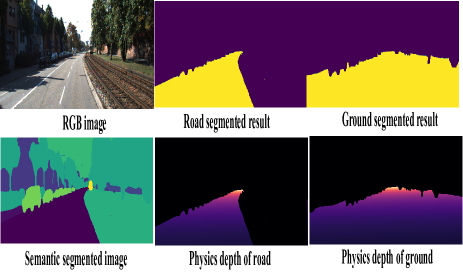
Figure 2: Physics Depth Methodology demonstrated on KITTI.

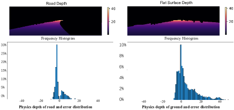
Figure 3: Error distribution of Physics depth.

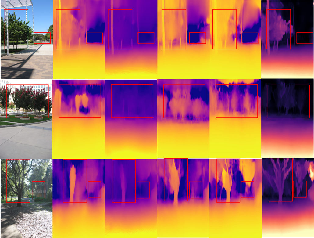
Figure 4: Qualitative results on make3d (Zero-shot): From left to right the models are Monodepth2  [12], RA-Depth  [16], MonoVit [37], SQLDepth [33], our models.

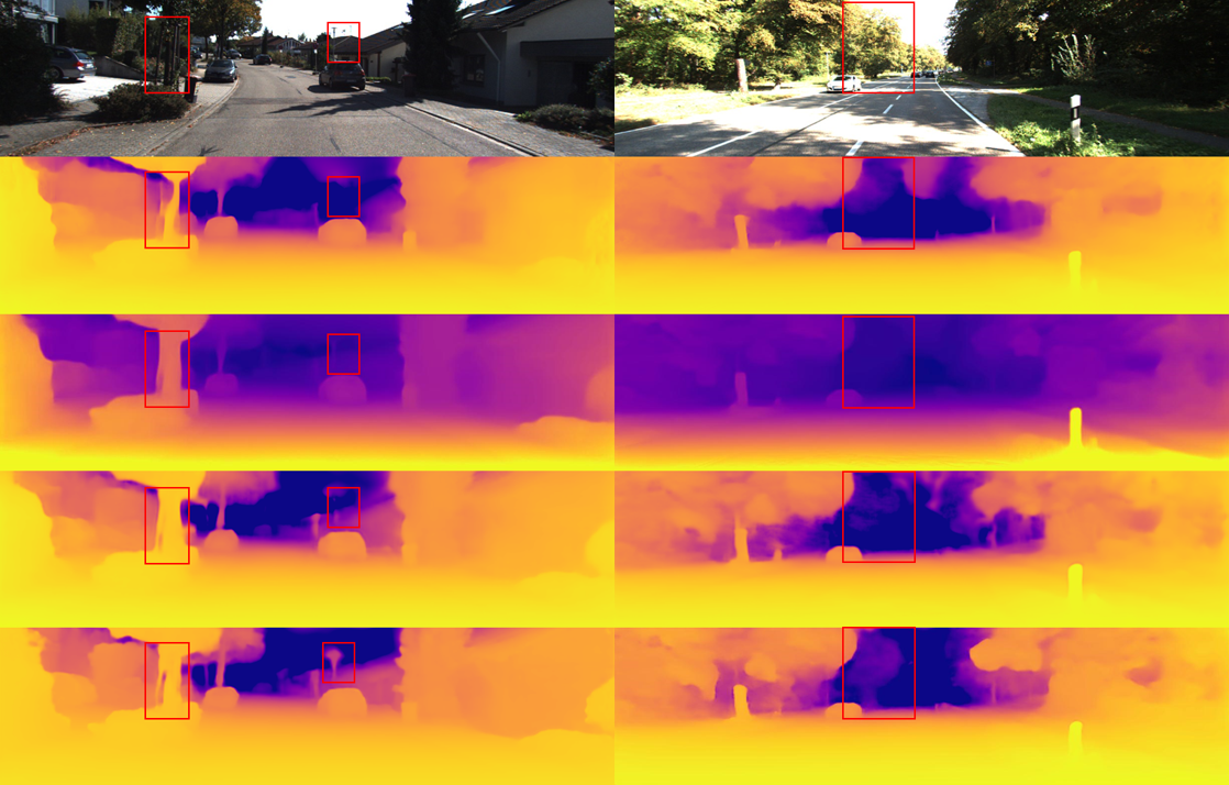
Figure 5: Qualitative results on KITTI: From top to bottom the models are MonoVit [37], RA-Depth  [16], ManyDepth [34], our models.

V-C Evaluation of Physics Depth

In this paper, we have systematically generated physics depth for the entire KITTI and Cityscapes datasets to facilitate the training of our models. This involved a meticulous analysis of the discrepancies in both road and flat surface physics depth across these datasets. As detailed in Tables II and III, the KITTI dataset showed approximately $90\%$ of pixels exhibited an error margin of less than $10\%$, and about $80\%$ of pixels were within a mere $5\%$ deviation when compared with the LiDAR-generated depth. Notably, the Cityscapes dataset demonstrated exceptional performance. In this dataset, around $95\%$ of pixels showed less than a $10\%$ error margin, and $85\%$ of pixels were within a $5\%$ error range, in comparison to the depth derived from Cityscapes’ standard disparity data.

Tables II and III indicate that the road physics depth outperforms the flat surface physics depth in accuracy. Yet, road pixels in a single image are limited. To increase the density of physics depth pixels in each image, we applied the logic to flat surfaces, although the flatness of these surfaces is not exactly the same. This extension, while increasing data, also enlarges the error margin with the ground truth. Still, as seen in Tables II and III, the flat surface physics depth, despite higher errors, maintains good accuracy, enriching the dataset and reducing the risk of overfitting.

Our analysis showed that the KITTI dataset had lower accuracy than Cityscapes, likely due to differences in camera calibration quality. KITTI uses one calibration file per day, while Cityscapes has individual files for each image, suggesting that better calibration enhances physics depth accuracy. This implies that improved calibration could further increase the accuracy of physics depth. Our physics depth estimation method, especially for flat surfaces like roads, shows promising potential, replacing LiDAR in calculating scale factors for self-supervised monocular depth estimation.

V-D Depth Estimation

KITTI: Our model was assessed on the KITTI Eigen split of 697 images, and the results, displayed in Table V, demonstrate that our method significantly surpasses existing self-supervised techniques on the KITTI dataset. Our advancements, such as physics depth, confidence metrics, and 2D consistency checks, have notably enhanced performance, particularly in RMSE metrics. Figure 5 illustrates our model’s exceptional capability in capturing complex scene details and reconstructing scenes more accurately than other models like MonoVit, RA-Depth, and ManyDepth.

Cityscapes: To assess the generalizability of our model, we showcase results from the Cityscapes dataset. In Table VI, we perform additional comparisons where we train and test on the Cityscapes dataset. We consistently outperform competing methods.

Make3D: We evaluated our model’s generalization capabilities through a zero-shot test on the Make3D dataset, using a version pretrained on KITTI. Results in Table VII show that our model achieves lower errors than other zero-shot competitors, highlighting its superior zero-shot generalization. Figure 4 demonstrates that our model surpasses baseline models, producing high-quality depth with improved sharpness and scene detail accuracy, proving its exceptional ability to adapt to new scenarios without further fine-tuning.

V-E Ablation Study

Our ablation study, presented in Table VIII, evaluates the impact of various components in monocular depth estimation. Results indicate that integrating all components enhances performance compared to the baseline model.

Physics Depth: Table VIII shows that accurate ground depth significantly improves depth prediction, which is essential for precise object positioning and overall scene understanding. This enhancement in spatial perception not only clarifies size and distance ambiguities but also accelerates the model’s training and its ability to adapt to the geometry of diverse scenes.

Confidence in Physics Depth: As shown in Table VIII, our method, which assigns confidence scores to physics depth estimation, surpasses basic physics depth. Incorporating confidence scores enables our model to focus on more accurate regions during training, reducing error impact and improving self-supervision efficacy.

2D Spatial Consistency: Table VIII indicates that our model, which utilizes optical flow for 2D reprojection error calculation, outperforms the baseline model that relies solely on photometric consistency.

Our ablation study reveals that incorporating Physics Depth significantly enhances monocular depth estimation accuracy by initiating training with accurate ground depth. This self-supervised method, which emphasizes reliable Physics Depth areas, outperforms traditional approaches. Additionally, adding 2D Spatial Consistency further boosts accuracy.

VI Conclusion

This paper presents a novel self-supervised learning approach that integrates the physical characteristics of the camera model with the concept of embodiment, embedding them into the deep learning model. By leveraging physics-based depth cues, our method improves monocular depth estimation. Through the incorporation of physics depth estimation, our approach achieves an embodied understanding of the interaction between the camera and the physical world, enhancing the model’s accuracy and its ability to capture environmental details, surpassing existing self-supervised techniques. This method enables the model to accurately predict scene depth, achieving state-of-the-art self-supervised learning results on the KITTI, Cityscapes, and Make3D datasets. This approach provides better depth information, thereby deepening the model’s embodied understanding of real-world scenes.

References

- [1] Antyanta Bangunharcana, Ahmed Magd, and Kyung-Soo Kim. Dualrefine: Self-supervised depth and pose estimation through iterative epipolar sampling and refinement toward equilibrium. In CVPR, 2023.
- [2] Shariq Farooq Bhat, Ibraheem Alhashim, and Peter Wonka. Adabins: Depth estimation using adaptive bins. In CVPR, 2021.
- [3] Vincent Casser, Soeren Pirk, Reza Mahjourian, and Anelia Angelova. Unsupervised monocular depth and ego-motion learning with structure and semantics. In CVPR Workshops, 2019.
- [4] Hemang Chawla, Arnav Varma, Elahe Arani, and Bahram Zonooz. Multimodal scale consistency and awareness for monocular self-supervised depth estimation. In ICRA. IEEE, 2021.
- [5] Marius Cordts, Mohamed Omran, Sebastian Ramos, Timo Rehfeld, Markus Enzweiler, Rodrigo Benenson, Uwe Franke, Stefan Roth, and Bernt Schiele. The cityscapes dataset for semantic urban scene understanding. In CVPR, 2016.
- [6] David Eigen, Christian Puhrsch, and Rob Fergus. Depth map prediction from a single image using a multi-scale deep network. NeurIPS, 27, 2014.
- [7] David Gallup, Jan-Michael Frahm, and Marc Pollefeys. Piecewise planar and non-planar stereo for urban scene reconstruction. In CVPR. IEEE, 2010.
- [8] Divyansh Garg, Yan Wang, Bharath Hariharan, Mark Campbell, Kilian Q Weinberger, and Wei-Lun Chao. Wasserstein distances for stereo disparity estimation. NeurIPS, 33, 2020.
- [9] Ravi Garg, Vijay Kumar Bg, Gustavo Carneiro, and Ian Reid. Unsupervised cnn for single view depth estimation: Geometry to the rescue. In Computer Vision–ECCV 2016: 14th European Conference, Amsterdam, The Netherlands, October 11-14, 2016, Proceedings, Part VIII 14. Springer, 2016.
- [10] Andreas Geiger, Philip Lenz, Christoph Stiller, and Raquel Urtasun. Vision meets robotics: The kitti dataset. IJRR, 32, 2013.
- [11] Clément Godard, Oisin Mac Aodha, and Gabriel J Brostow. Unsupervised monocular depth estimation with left-right consistency. In CVPR, 2017.
- [12] Clément Godard, Oisin Mac Aodha, Michael Firman, and Gabriel J Brostow. Digging into self-supervised monocular depth estimation. In ICCV, 2019.
- [13] Vitor Guizilini, Rares Ambrus, Sudeep Pillai, Allan Raventos, and Adrien Gaidon. 3d packing for self-supervised monocular depth estimation. In CVPR, 2020.
- [14] Caner Hazirbas, Lingni Ma, Csaba Domokos, and Daniel Cremers. Fusenet: Incorporating depth into semantic segmentation via fusion-based cnn architecture. In ACCV. Springer, 2017.
- [15] Kaiming He, Xiangyu Zhang, Shaoqing Ren, and Jian Sun. Deep residual learning for image recognition. In CVPR, 2016.
- [16] Mu He, Le Hui, Yikai Bian, Jian Ren, Jin Xie, and Jian Yang. Ra-depth: Resolution adaptive self-supervised monocular depth estimation. In ECCV. Springer, 2022.
- [17] Uday Kusupati, Shuo Cheng, Rui Chen, and Hao Su. Normal assisted stereo depth estimation. In CVPR, 2020.
- [18] Seokju Lee, Sunghoon Im, Stephen Lin, and In So Kweon. Learning monocular depth in dynamic scenes via instance-aware projection consistency. In AAAI, volume 35, 2021.
- [19] Seokju Lee, Francois Rameau, Fei Pan, and In So Kweon. Attentive and contrastive learning for joint depth and motion field estimation. In CVPR, 2021.
- [20] Yinhao Li, Zheng Ge, Guanyi Yu, Jinrong Yang, Zengran Wang, Yukang Shi, Jianjian Sun, and Zeming Li. Bevdepth: Acquisition of reliable depth for multi-view 3d object detection. In AAAI, volume 37, 2023.
- [21] Xiaoxiao Long, Cheng Lin, Lingjie Liu, Wei Li, Christian Theobalt, Ruigang Yang, and Wenping Wang. Adaptive surface normal constraint for depth estimation. In ICCV, 2021.
- [22] Guoyu Lu. Deep unsupervised visual odometry via bundle adjusted pose graph optimization. In ICRA, pages 6131–6137, 2023.
- [23] Guoyu Lu, Yan Yan, Li Ren, Philip Saponaro, Nicu Sebe, and Chandra Kambhamettu. Where am i in the dark: Exploring active transfer learning on the use of indoor localization based on thermal imaging. Neurocomputing, 173:83–92, 2016.
- [24] Guoyu Lu, Yan Yan, Li Ren, Jingkuan Song, Nicu Sebe, and Chandra Kambhamettu. Localize me anywhere, anytime: a multi-task point-retrieval approach. In ICCV, pages 2434–2442, 2015.
- [25] Xiaoyang Lyu, Liang Liu, Mengmeng Wang, Xin Kong, Lina Liu, Yong Liu, Xinxin Chen, and Yi Yuan. Hr-depth: High resolution self-supervised monocular depth estimation. In AAAI, volume 35, 2021.
- [26] Reza Mahjourian, Martin Wicke, and Anelia Angelova. Unsupervised learning of depth and ego-motion from monocular video using 3d geometric constraints. In CVPR, 2018.
- [27] Andrea Pilzer, Dan Xu, Mihai Puscas, Elisa Ricci, and Nicu Sebe. Unsupervised adversarial depth estimation using cycled generative networks. In 3DV. IEEE, 2018.
- [28] Daniel Scharstein and Richard Szeliski. A taxonomy and evaluation of dense two-frame stereo correspondence algorithms. International journal of computer vision, 47, 2002.
- [29] Yang Tang, Chaoqiang Zhao, Jianrui Wang, Chongzhen Zhang, Qiyu Sun, Wei Xing Zheng, Wenli Du, Feng Qian, and Juergen Kurths. Perception and navigation in autonomous systems in the era of learning: A survey. TNNLS, 2022.
- [30] Alexandru Telea. An image inpainting technique based on the fast marching method. Journal of graphics tools, 9, 2004.
- [31] Chaoyang Wang, José Miguel Buenaposada, Rui Zhu, and Simon Lucey. Learning depth from monocular videos using direct methods. In CVPR, 2018.
- [32] Ruoyu Wang, Zehao Yu, and Shenghua Gao. Planedepth: Self-supervised depth estimation via orthogonal planes. In CVPR, 2023.
- [33] Youhong Wang, Yunji Liang, Hao Xu, Shaohui Jiao, and Hongkai Yu. Sqldepth: Generalizable self-supervised fine-structured monocular depth estimation. arXiv preprint arXiv:2309.00526, 2023.
- [34] Jamie Watson, Oisin Mac Aodha, Victor Prisacariu, Gabriel Brostow, and Michael Firman. The temporal opportunist: Self-supervised multi-frame monocular depth. In CVPR, 2021.
- [35] Jiaxing Yan, Hong Zhao, Penghui Bu, and YuSheng Jin. Channel-wise attention-based network for self-supervised monocular depth estimation. In 3DV. IEEE, 2021.
- [36] Ning Zhang, Francesco Nex, George Vosselman, and Norman Kerle. Lite-mono: A lightweight cnn and transformer architecture for self-supervised monocular depth estimation. In CVPR, 2023.
- [37] Chaoqiang Zhao, Youmin Zhang, Matteo Poggi, Fabio Tosi, Xianda Guo, Zheng Zhu, Guan Huang, Yang Tang, and Stefano Mattoccia. Monovit: Self-supervised monocular depth estimation with a vision transformer. In 3DV. IEEE, 2022.
- [38] Tinghui Zhou, Matthew Brown, Noah Snavely, and David G Lowe. Unsupervised learning of depth and ego-motion from video. In CVPR, 2017.