Discriminating among cosmological models by data-driven methods

Abstract

Background: The study explores the Pantheon+SH0ES dataset to identify patterns that can discriminate between different cosmological models. It focuses on determining whether the behaviour of dark energy is consistent with the standard $\Lambda$CDM model or suggests novel cosmological features.

Methods: The central goal is to evaluate the robustness of the $\Lambda$CDM model compared with other dark energy models, and to investigate whether there are deviations that might indicate new cosmological insights. The study takes into account a data-driven approach, using both traditional statistical methods and machine learning techniques. Initially, we evaluate six different dark energy models using traditional statistical methods like Markov Chain Monte Carlo (MCMC), Static and Dynamic Nested Sampling to infer the cosmological parameters. Subsequently, we adopt a machine learning approach, developing a regression model to compute the distance modulus of each supernova, expanding the feature set to 74 statistical features. The machine learning approach uses an ensemble of four different models: MultiLayer Perceptron, k-Nearest Neighbours, Random Forest Regressor, and Gradient Boosting. In four scenarios, cosmological parameters are estimated by using MCMC and Nested Sampling. Feature selection techniques (Random Forest, Boruta, SHAP) are used in three scenarios. This procedure mirrors the initial phase of the study.

Results: Traditional statistical analysis confirms that the $\Lambda$CDM model is robust, yielding expected parameter values. Other models show deviations, with the Generalised and Modified Chaplygin Gas models performing poorly. In the machine learning analysis, feature selection techniques, particularly Boruta, significantly improve model performance. In particular, models initially considered weak (Generalised/Modified Chaplygin Gas) show significant improvement after feature selection.

Conclusions: The study demonstrates the effectiveness of a data-driven approach to cosmological model evaluation. The $\Lambda$CDM model remains robust, while machine learning techniques, in particular feature selection, reveal potential improvements in alternative models which could be relevant for new observational campaigns like the recent DESI survey.

I Introduction

At the turn of the 21st century, a significant breakthrough in our comprehension of the cosmos occurred, thanks to two separate teams of cosmologists. The Supernova Cosmology Project [1], and the High-Z Supernovae Search Team [2] inaugurated a new era of cosmic understanding. By studying far-off Type Ia Supernovae, they uncovered a universe that was expanding at an accelerated pace. The groundbreaking discovery necessitated a re-evaluation of longstanding cosmic assumptions and triggered the development of new models. Most of them are related to the concept of dark energy [3], a cosmic enigma hypothesised to account for the observed accelerated expansion (see [4] for a review). Einstein’s General Relativity, when applied to cosmology sourced by baryonic matter and radiation, cannot explain such an accelerated dynamics. As a result, new hypotheses regarding dark energy [5] or extensions of General Relativity [6] have become imperative. The $\Lambda$CDM model, which revisits Einstein’s original concept of a cosmological constant, has emerged as a strong contender for explaining accelerated dynamics [7]. This model has revived the repulsive gravitational impact of the cosmological constant as a credible means of explaining cosmic acceleration. In terms of particle physics, the cosmological constant $\Lambda$ is representative of vacuum energy [8]. Thus, the quest for a mechanism yielding a small, observationally consistent value for the cosmological constant remains paramount. Distinguishing among the myriad dark energy models necessitates the establishment of observational constraints, often derived from phenomena such as Type Ia Supernovae, Cosmic Microwave Background (CMB) radiation, and large-scale structure observations. A key objective to deal with dark energy is identifying any potential deviations in the value of the parameter

$$w_{\text{de}}=\frac{p_{\text{de}}}{\rho_{\text{de}}},$$ (1)

where $p_{\text{de}}$ is the pressure of dark energy and $\rho_{\text{de}}$ is its energy density, from its standard value of

$$w_{\Lambda}=-1,$$ (2)

and to determine whether it aligns with the cosmological constant or diverges at some cosmic scale.

The present study is devoted to this issue. The aim is to show that concurring dark energy cosmological models can be automatically discriminated applying machine learning techniques to suitable samples of data.

The paper consists of two interconnected yet distinct parts. The initial section focuses on Bayesian inference using sampling techniques, specifically Monte Carlo Markov Chains (MCMC) [9] and Nested Sampling [10], applied to the original data set.

MCMC is a versatile method that can be used to sample from any probability distribution. Its primary use is for sampling from hard-to-handle posterior distributions in Bayesian inference. In Bayesian estimation, computing the marginalized probability can be computationally expensive, especially for continuous distributions. The key advantage of MCMC is its ability to bypass the calculation of the normalization constant. The general idea of the algorithm involves initiating a Markov chain with a random probability distribution over states. It gradually converges towards the desired probability distribution. The algorithm relies on a condition (Detailed Balance Sheet) to ensure that the stationary distribution of the Markov chain approximates the posterior probability distribution.

If this condition is satisfied, it guarantees that the stationary state of the Markov chain approximates the posterior distribution. Although MCMC is a complex method, it offers great flexibility, allowing efficient sampling in high-dimensional spaces and solving problems with large state spaces. However, it has a limitation: MCMC is poor at approximating probability distributions with multiple modes.

The Nested Sampling algorithm (NS) was introduced by Skilling in 2004 within the domain of Bayesian inference and computation. This algorithm addresses the challenges posed by high-dimensional integrals by guiding a set of live points through the parameter space.

The NS algorithm gained rapid adoption in cosmology due to its ability to partially overcome three significant issues encountered in the conventional Bayesian computation method, the MCMC. Firstly, it provides simultaneous results for both model comparison and parameter inference. Secondly, it demonstrates success in handling multi-modal problems. Thirdly, it has a built-in self-tuning capability, allowing immediate application to new problems.

In our work, we are going to use two versions of NS: one with a fixed number of live points, called Static Nested Sampling, and one with a varying number of live points during runtime, called Dynamic Nested Sampling.

By using redshift and distance modulus data, the study explores six dark energy models:

1. $\Lambda$CDM: the standard model.

2. Linear Redshift [11, 12]: that propose a linear relation between redshift and w. It is the simplest possible parameterisation.

3. Chevallier-Polarski-Linder [13, 14] (CPL): simple, but flexible and robust parameterisation that tries to cover the over-all time evolution of w.

4. Squared Redshift [15]: this model propose a squared relation between redshift and w and covers the universe redshift regions where the CPL parameterisation fails.

5. Generalized Chaplygin Gas [16] (GCG): is the first scenario that we will investigate where dark matter and dark energy are unified.

6. Modified Chaplygin Gas [17] (MCG): is a modified version of the previous parameterisation and has the largest number of free parameters among the models we studied, three.

In the second section of this study, inspired by the work of D’Isanto et al. [18] and the FATS public Python library [19], we are going to compute additional statistics for each supernova and to use three feature selection techniques to identify significant parameters from a final set of $70$ features. In fact, as we will see, it is possible to analyze four different cases: a ’base’ case where no feature selection is used; a case where the first 18 features selected by Random Forest are taken [20]; a case where the feature selection method used is Boruta [21]; and a last case where the first 18 features selected by SHAP are taken into account [22]. An ensemble learning strategy is then utilised to create a predictive model for the distance modulus based on the selected features. The models we are going to use in the ensemble learning are the following:

1. MultiLayer Perceptron [23] (MLP): a modern feedforward artificial neural network, consisting of fully connected neurons with a non-linear kind of activation function.

2. k-Nearest Neighbours [24] (k-NN): a non-parametric supervised learning method used for both classification and regression.

3. Random Forest Regressor [25]: an ensemble learning method for classification, regression and other tasks that operates by constructing a multitude of decision trees at training time. For regression tasks, the mean or average prediction of the individual trees is returned.

4. Gradient Boosting [26]: a machine learning technique used in regression and classification tasks, among others. It gives a prediction model in the form of an ensemble of weak prediction models, i.e. models making very few assumptions about the data, which are typically simple decision trees [27]. When a decision tree is the weak learner, the resulting algorithm is called gradient-boosted trees [28].

Subsequently, the new dataset, composed by original redshifts and predicted distance moduli, is subjected to the same sampling techniques previously used in the derivation of cosmological parameters.

The paper is structured as follows: Section II outlines the six dark energy models analysed. In Section III, the data set is presented. We describe the compilation of Pantheon+SH0ES and the new features that have been added. Section IV focuses on feature selection techniques used and the models implemented in our ensemble learning. In Section V, the different sampling techniques are described in detail, with an explanation of the specifics of MCMC and NS for the inference of cosmological parameters. We conclude with a brief introduction to the information criteria used to evaluate the performance of the techniques. Section VI presents the results of the study, showing the insights gained by implementing traditional Bayesian inference techniques as well as machine learning and sampling methods. Finally, in Section VII, we summarize our conclusions and present some perspectives of the approach.

II Dark energy models

There are several alternatives proposed to the $\Lambda$CDM model, ranging from adding phenomenological dark energy terms to modifying the Hilbert-Einstein action or considering other geometrical invariants [29]. To refine the model with dark energy evolving over time, a barotropic factor $\omega(z)=P/\rho$ dependent on $z$ can be considered. This is the equation of state (EoS) of the given cosmological model. However, this approach has a crucial aspect: it is not possible to define $\omega(z)$ a priori; it must be reconstructed starting from observations. As stated in Dunsby and Luongo [30], it is advantageous to express the barotropic factor in terms of cosmic time or, more appropriately, as a function of the scale factor or redshift. This choice is based on the idea that dark energy could evolve through a generic function over the history of the universe. In this sense, the cosmographic analysis can greatly help in reconstructing the cosmic flow by the choice of suitable polynomials in the redshift $z$ (see e.g. [31, 32, 33, 34, 35]). A straightforward approach involves expanding $\omega$ as a Taylor series in redshift $z$:

$$\omega(z)=\sum_{n=0}^{\infty}\omega_{n}z^{n}.$$ (3)

However, opting for this expansion could pose challenges, as it may lead to a divergence in the equation of state at higher redshifts.

The following paragraphs present the six models studied in this paper.

II.1 $\Lambda$CDM

It is the standard model where $w=-1$ and the Hubble function is:

$$E(z)^{2}=\left(\frac{H(z)}{H_{0}}\right)^{2}=\Omega_{m}(1+z)^{3}+(1-\Omega_{m}).$$ (4)

The $\Lambda$CDM model provides a good fit for a large number of observational data sets but does not solve some important problems like the cosmic coincidence or the fine tuning of the $\Lambda$ value.

II.2 Linear Redshift

It is the simplest parameterisation and consists of a linear relation between the redshift and the $w$ which takes the following form:

$$w(z)=w_{0}-w_{a}z,$$ (5)

where $w_{0}$ and $w_{a}$ (or $w_{z}$) are constants. Here $w_{0}$ represents the present value of $w(z)$. The model can be reduced to the $\Lambda$CDM model for $w_{0}=-1$ and $w_{a}=0$. In this parameterisation, the Hubble function takes the form:

$$E(z)^{2}=\Omega_{m}(1+z)^{3}+\Omega_{x}(1+z)^{3(1+w_{0}+w_{a})}e^{-3w_{a}z},$$ (6)

where $\Omega_{m}$ is the density parameter for perfect fluid matter, while $\Omega_{x}$ is the density parameter associated with dark energy. However, this ansatz diverges at high redshift and consequently needs for strong constraints on $w_{a}$ in studies involving data at high redshifts, e.g., when we use CMB data [36].

II.3 Chevallier-Polarski-Linder

The CPL model is a simple parameterisation that shows interesting properties and can be represented by two parameters that exhibit the present value of the EoS ($w_{0}$) and its over-all time evolution is:

$$w(z)=w_{0}+\frac{z}{1+z}w_{a}.$$ (7)

Within this model, the Hubble function now takes the following form [37]:

$$E(z)^{2}=\Omega_{m}(1+z)^{3}+\Omega_{x}(1+z)^{3(1+w_{0}+w_{a})}e^{-\frac{3w_{a}z}{1+z}}.$$ (8)

The CPL parameterisation is one of the most flexible and robust parameterisations of the Dark Energy EoS.

II.4 Squared Redshift

This model brings a step forward in redshift regions where the Chevallier-Polarski-Linder (CPL) parameterisation cannot be extended to the entire history of the universe. Its functional form is given by:

$$w(z)=w_{0}+\frac{z(1+z)}{1+z^{2}}w_{a},$$ (9)

which is well-behaved at $z\to-1$. Here, the Hubble function takes the following form:

$$E(z)^{2}=\Omega_{m}(1+z)^{3}+(1-\Omega_{m})(1+z)^{3(1+w_{0})}(1+z^{2})^{\frac{3w_{a}}{2}}.$$ (10)

In summary, the squared redshift model has the advantage of being a limited function of z throughout the entire history of the Universe.

II.5 Unified Dark Energy Fluid scenarios

As an extension of established scenarios within the homogeneous and isotropic universe framework, we posit that the gravitational sector, minimally coupled to the matter sector, adheres to standard General Relativity. Additionally, we postulate that the total energy content of the universe consists of photons ($\gamma$), baryons ($b$), neutrinos ($\nu$), and a unified dark fluid (UDF, $X_{U}$) [38, 39]. This UDF can exhibit characteristics of dark energy, dark matter, or a distinct fluid type during the universe expansion. Thus, the comprehensive energy budget is denoted by $\rho_{i}$, where $i=\gamma,b,\nu,X_{U}$. Moreover, each fluid $i$ follows a continuity equation given by $\dot{\rho_{i}}+3\frac{\dot{a}}{a}(\rho_{i}+p_{i})=0$. Standard solutions include $\rho_{b}\propto a^{-3}$ and $\rho_{\gamma,\nu}\propto a^{-4}$. For the UDF, we assume a constant adiabatic sound speed $c_{s}$ and model it as $p=c_{s}^{2}(\rho-\tilde{\rho})$, where $c_{s}$ and $\tilde{\rho}$ are positive constants [40]. A part of this expression behaves akin to the typical barotropic cosmic fluid, while the other emulates $\Lambda$, unifying the dark energy and dark matter components (a phenomenon known as dark degeneracy). By integrating the UDF equation, we obtain:

$$\rho=\rho_{\Lambda}+\rho_{X_{U}}a^{-3(1+c_{s}^{2})},$$ (11)

$$p=-\rho_{\Lambda}+c_{s}^{2}\rho_{X_{U}}a^{-3(1+c_{s}^{2})},$$ (12)

where $\rho_{\Lambda}=c_{s}^{2}\tilde{\rho}/(1+c_{s}^{2})$ and $\rho_{X_{U}}=\rho_{0}-\rho_{\Lambda}$, with $\rho_{0}$ as the dark energy density at present time. The dynamical EoS is given by:

$$w=-1+\frac{1+c_{s}^{2}}{\left(\frac{\rho_{\Lambda}}{\rho_{X_{U}}}\right)(1+z)^{-3(1+c_{s}^{2})}+1}.$$ (13)

At this point, a specific form which specifies $p_{X_{U}}$ as a function of $\rho_{X_{U}}$: $p_{X_{U}}=f(\rho_{X_{U}})$ needs to be considered.

II.5.1 Generalised Chaplygin gas

In the GCG model, for a given $X_{U}$, we have:

$$p_{\text{gcg}}=-\frac{A}{(\rho_{\text{gcg}})^{\alpha}},$$ (14)

where $A$ and $0\leq\alpha\leq 1$ are two free parameters. The case $\alpha=1$ corresponds to the original Chaplygin gas model. Solving the continuity equation using the evolution of the GCG energy density, one gets:

$$\rho_{\text{gcg}}(a)=\rho_{\text{gcg},0}\left[b+(1-b)a^{-3(1+\alpha)}\right]^{\frac{1}{1+\alpha}},$$ (15)

where $\rho_{\text{gcg},0}$ denotes the energy density of the GCG fluid at present time and $b=A\rho_{\text{gcg},0}^{-(1+\alpha)}$. This density contains all the $i$ components described above. Then we can compute the GCG dynamical EoS $w_{\text{gcg}}$ as a function of the redshift $z$:

$$w_{\text{gcg}}(z)=-\frac{b}{b+(1-b)\left(\frac{1}{1+z}\right)^{-3(1+\alpha)}}.$$ (16)

This establishes the regions of dominations for an effective dark matter component and an effective dark energy one, with an intermediate region for $\alpha=1$.

II.5.2 Modified Chaplygin gas

Here, the relation between pressure $p_{\text{mcg}}$ and energy density $\rho_{\text{mcg}}$ is given by:

$$p_{\text{mcg}}=b\rho_{\text{mcg}}-\frac{A}{(\rho_{\text{mcg}})^{\alpha}},$$ (17)

where again $A$, $b$, and $\alpha$ are three real constants with $0\leq\alpha\leq 1$. If $A=0$, the MCG behaves as a perfect fluid with $w=b$, whereas, if $b=0$, we can recover the GCG model. Again, the standard Chaplygin gas model can be obtained by setting $\alpha=0$. Solving the equation, we find the evolution of the MCG energy density with all its $i$ components:

$$\rho_{\text{mcg}}(a)=\rho_{\text{mcg},0}\left[b_{s}+(1-b_{s})a^{-3(1+b)(1+\alpha)}\right]^{\frac{1}{1+\alpha}},$$ (18)

where $\rho_{\text{mcg},0}$ denotes the energy density of the MCG fluid at present time, and $b_{s}=A\rho_{\text{gcg},0}^{-(1+\alpha)}/(1+b)$. The evolution of the MCG EoS is given by:

$$w_{\text{mcg}}(z)=b-\frac{b_{s}(1+b)}{b_{s}+(1-b_{s})\left(\frac{1}{1+z}\right)^{-3(1+b)(1+\alpha)}}.$$ (19)

As an extension of the GCG model, the MCG model behaves accordingly with each cosmological region described. It is worth saying that Chaplygin gas models can be taken into account to investigate in details the dark side behaviour both at early and late cosmic epochs [41]. The interaction between the dark components can be considered also to track the whole cosmic history [42].

III Data Set

As mentioned, the used dataset is the Pantheon+SH0ES of 1701 Type Ia Supernovae coming from a compilation of 18 different surveys covering a redshift range up to 2.26. Among the 1701 objects in the dataset, 151 are duplicates, observed in multiple surveys, and 12 are pairs or triplets of SN siblings, SNe found in the same host galaxy.

The number of features provided by the Pantheon+SH0ES dataset is 45, excluding the ID of the supernova, the ID of the survey used for that observation, and a binary variable to distinguish the SNe used in SH0ES from those not included. However, we decided to use more features to gain more confidence in the forthcoming results, and so we added a number of statistical features from D’Isanto et al. [18] and the FATS Python library, bringing the total number of our features to 71 (still excluding the previously cited features). For more information on this statistical parameter space, see the Appendix.

III.1 The Pantheon+SH0ES compilation

The dataset comprises 1701 Type Ia Supernovae (SNeIa) sourced from 18 surveys, spanning a redshift range from 0.001 to 2.26, making it the largest spectroscopically confirmed sample to date. SNeIa yield determinations of the distance modulus ($\mu$), which theoretically correlates with the luminosity distance ($d_{L}$) as:

$$\mu(z)=5\log{\frac{d_{L}(z)}{1\text{ Mpc}}}+25,$$ (20)

where $d_{L}$ is measured in Mpc. In standard statistical analyses, a nuisance parameter $M$ is added to $\mu$, representing an unknown offset accounting for the absolute magnitude of supernovae (and other possible systematics), which is degenerate with $H_{0}$.

Assuming spatial flatness, the luminosity distance is related to the comoving distance ($D$) by:

$$d_{L}(z)=\frac{c}{H_{0}}(1+z)D(z),$$ (21)

where $c$ is the speed of light. Thus, the normalized Hubble function ($H(z)/H_{0}$) can be computed by taking the inverse of the derivative of $D(z)$ with respect to the redshift:

$$D(z)=\frac{H_{0}}{c}\int_{0}^{z}\frac{d\tilde{z}}{H(\tilde{z})},$$ (22)

where $H_{0}$ is considered a prior value for normalizing $D(z)$.

IV Methods

In our study, we use three different feature selection techniques to identify significant parameters from a final set of 70 features. Our analysis includes four different cases: a baseline scenario with no feature selection, a scenario using the first 18 features selected by Random Forest, a scenario using Boruta feature selection, and a scenario using the first 18 features selected by SHAP. We then use an ensemble learning approach to develop a predictive model for the distance modulus based on the selected features. The ensemble consists of four models: MultiLayer Perceptron (MLP), k-Nearest Neighbours (k-NN), Random Forest Regressor and Gradient Boosting. Each of these models brings unique capabilities to the ensemble, from the flexible architecture of MLP to the non-parametric nature of k-NN, the ensemble learning of Random Forest, and the gradient-boosted trees approach of Gradient Boosting.

IV.1 Feature selection techniques

Feature selection is a crucial step in the process of building machine learning models, playing a pivotal role in enhancing model performance, interpretability, and efficiency. In many real-world scenarios, datasets often contain a multitude of features, and not all of them contribute equally to the predictive task at hand. Some features may even introduce noise or lead to computational inefficiencies.

IV.1.1 Random Forest

In the building of the single Decision Trees, the feature selected at each node is the one which minimize the chosen loss function (like the mean squared error in our case). Feature importance in a Random Forest is calculated based on how much each feature contributes to the reduction in loss function across all the trees in the ensemble. The more frequently a feature is used to split the data and the higher the loss function reduction it achieves, the more important it is considered. In Random Forests, the impurity, or loss function, decrease from each feature can be averaged across trees to determine the final importance of the variable. To give a better intuition, features that are selected at the top of the trees are in general more important than features that are selected at the end nodes of the trees, as generally the top splits lead to bigger information gains [20].

IV.1.2 Boruta

The second method used is an all-relevant feature selection method, or Boruta. The Boruta algorithm takes its name from a demon in Slavic mythology who lived in pine forests and preyed on victims by walking like a shadow among the trees. And, in fact, main concept behind this method is the introduction of shadow features and the use of random forest as predicting model [21]. A shadow feature for each real one is introduced by randomly shuffling its values among the N samples of the given dataset. It uses a random forest classifier, and so is a feature selection wrapping method, on this extended data set (real and shadow features) and applies a feature importance measure such as Mean Decrease Accuracy and evaluates the importance of each feature. At every iteration, Boruta algorithm checks whether a real feature has a higher importance than the best of its shadow features and constantly removes features which are deemed highly unimportant. Finally, the Boruta algorithm stops either when all features gets confirmed or rejected or it reaches a specified limit of iterations.

In conclusion, the steps of this algorithm can be summarized like this:

1. Take the original features and make a shuffled copy. The new extended dataset is now composed by the original features and their shuffled copy, the shadow features.

2. Run a random forest classifier on this new dataset and calculate the feature importance of every feature.

3. Store the highest feature importance of the shadow features and use it as a threshold value.

4. Keep the original features which have an importance higher than the highest shadow feature importance. We will say that these features make a hit.

5. Repeat the previous steps for some iterations and keep track of the hits of the original features.

6. Label as confirmed or important the features that have a significantly high number of hits; as rejected the ones that instead have a significantly low number of hits; as tentative the ones that fall in between.

The algorithm stops when all features have an established decision, or when a pre-set maximal number of iterations is reached.

IV.1.3 SHAP

The final feature selection method used in our study was SHAP [22] (SHapley Additive exPlanations). SHAP adopts a game-theoretic approach to explain the output of machine learning models, connecting optimal credit allocation with local explanations using classic Shapley values from game theory and their related extensions. SHAP serves as a set of software tools designed to enhance the explainability, interpretability, and transparency of predictive models for data scientists and end-users [43]. SHAP is used to explain an existing model. In the context of a binary classification case built with a sklearn model, the process involves training, tuning, and testing the model. Subsequently, SHAP is employed to create an additional model that explains the classification model.

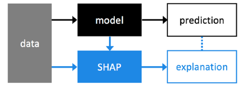
Figure 1: SHAP architecture [44].

The key components of a SHAP explanation include:

• explainer: the type of explainability algorithm chosen based on the model used.

• base value: it represents the value that would be predicted if no features were known for the current output, typically the mean prediction for the training dataset or the background set. Also called as reference value.

• SHAPley values: the average contribution of each feature to each prediction for each sample based on all possible features. It is a $(n,m)$ matrix, $n$ samples, $m$ features, that represents the contribution of each feature to each sample.

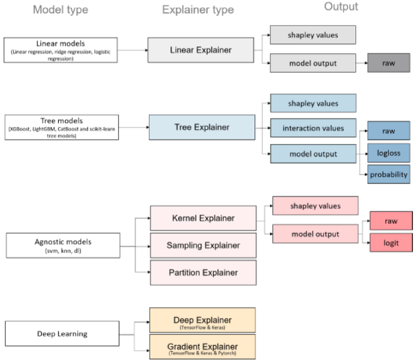
Figure 2: Types of Explainers [45].

Explainers are the models used to calculate shapley values. The diagram above (Figure 2) shows different types of Explainers. The choice of Explainers depends mainly on the selected learning model. The Kernel Explainer creates a model that substitutes the closest to our model. It also can be used to explain neural networks. For deep learning models, there are the deep and gradient Explainers. In our work we used a Tree Explainer. Shapley values calculate feature importance by evaluating what a model predicts with and without each feature. Since the order in which a model processes features can influence predictions, this comparison is performed in all possible ways to ensure fair assessments. This approach draws inspiration from game theory, and the resulting Shapley values facilitate the quantification of the impact of interactions between two features on predictions for each sample. As the Shapley values matrix has two dimensions (samples x features), interactions are represented as a tensor with three dimensions (samples x features x features).

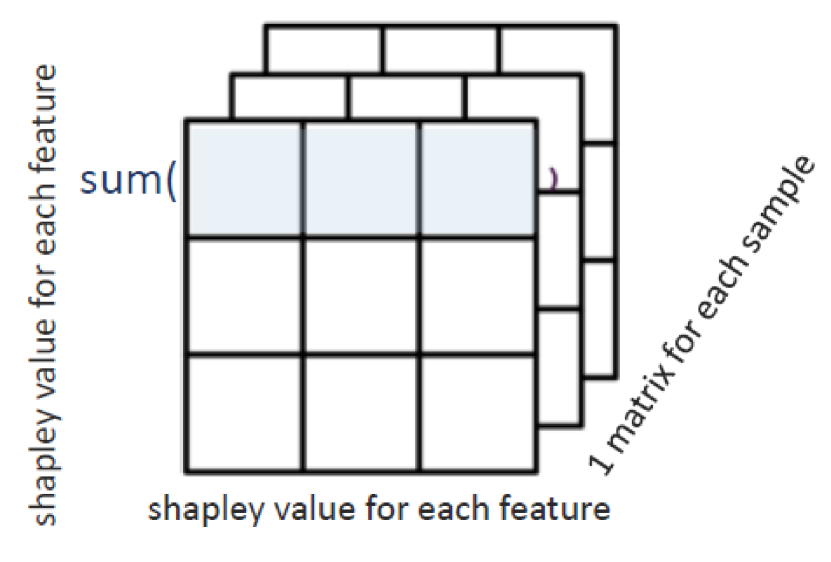
(a) Sum of row of matrix (features x features) equals SHAP value of this feature and this sample

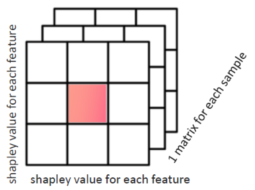
(b) The diagonal entries equals the main effect of this feature on the prediction

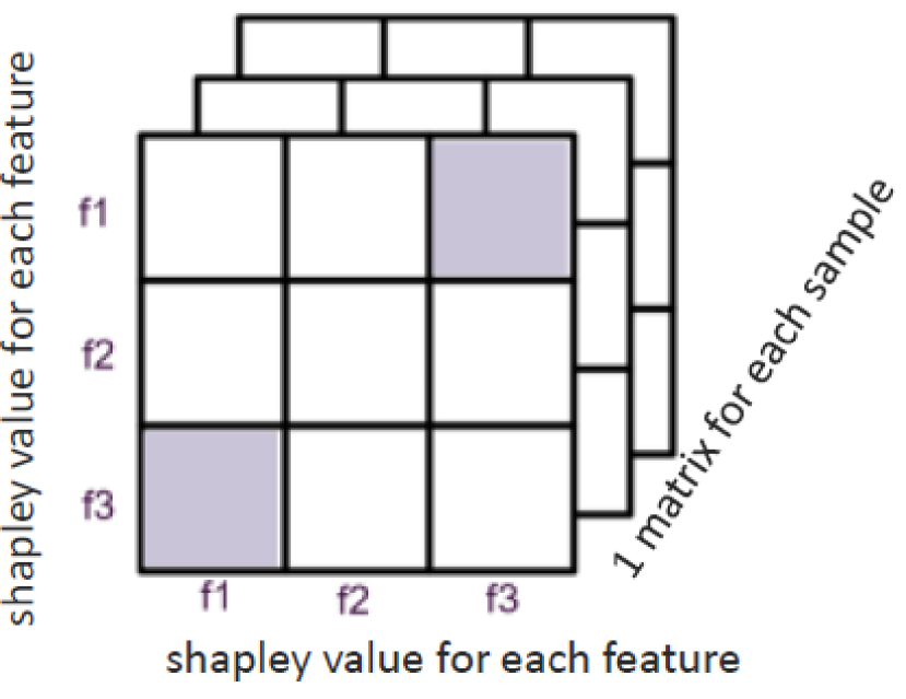
(c) The symmetrical entries out of the diagonal equals to the interaction effect between all the pairs of features for a given sample

Figure 3: SHAP matrix [45].

IV.2 Ensemble learning

From the plethora of different machine learning techniques available, the one used in this work is the Ensemble Learning. In this approach, two or more models are fitted on the same data and the predictions from each model are combined. The objective of ensemble learning is to achieve better performance with the ensemble of models as compared to any individual model. The models that compose the ensemble learning used in the work will be discussed in the following paragraphs.

IV.2.1 Multi Layer Perceptron

The MLP, or Multi Layer Perceptron, is the first of the four models used in the ensemble learning used in the work. The MLP is one of the most common used feed forward neural network model [46, 23, 47, 48] and comes from the profound limitations of the first Rosenblatt’s Perceptron in the treatment of non linearly separable, noisy and non numerical data. The term feed-forward refers to the fact that in this neural network model, the impulse is always propagated in the same direction, e.g. from the input layer to the output layer, passing through one or more hidden layers, by combining the sum of weights associated to all neurons except the input ones. The output of each neuron is obtained by an activation function applied to the weighted sum of the inputs. The shape of the activation function can vary considerably from model to model, from the simplest linear function to the hyperbolic tangent, which is the one used in this work. In the training phase of the network, the weights are modified according to the learning rule used, until a predetermined distance between the network output and the desired output is reached (usually this distance is decided a priori by the user and is commonly known as the Error Threshold).

The easiest way to employ gradient information is to choose the weight update to make small steps in the direction of the negative gradient, so that

$$\textbf{w}^{\tau+1}=\textbf{w}^{\tau}-\eta\nabla E(\textbf{w}^{\tau}),$$ (23)

where the parameter $\eta>0$ is referred to as the learning rate. In each iteration, the vector is adjusted in the direction of the steepest decrease of the error function, and this strategy is called gradient descent. We still need to define an efficient technique to find the gradient of the error function $E(w)$. A widely used method is the error backpropagation in which information is sent alternately forward and backward through the network. However, this method lacks precision and optimization for complex real-life applications. Therefore, modifications are necessary.

Adaptive Moment Estimation [49] (ADAM) takes a step forward in the pursuit of the minimum of the objective function by solving the problem of learning rate selection and avoiding saddle points. ADAM computes adaptive learning rates for each parameter and maintains an exponentially decaying average of past gradients. This average is weighted with respect to the first two statistical moments of the gradient distribution. Adam behaves like a heavy ball with friction, where $\widehat{m_{t}}$ and $\widehat{v_{t}}$ are the estimate of the first and second moment of the gradients, and are computed like this:

$$\widehat{m_{t}}=\frac{m_{t}}{1-\beta_{1}^{t}}=\frac{\beta_{1}m_{t-1}+(1-\beta_{1})\nabla_{w}f(W;x^{(i)}y^{(i)})}{1-\beta_{1}^{t}},$$ (24)

$$\widehat{v_{t}}=\frac{v_{t}}{1-\beta_{2}^{t}}=\frac{\beta_{2}v_{t-1}+(1-\beta_{2})\nabla_{w}f(W;x^{(i)}y^{(i)})^{2}}{1-\beta_{2}^{t}},$$ (25)

where $\beta_{1}$ and $\beta_{2}$ are the characteristic memory times of the first and second moment of the gradients and control the decay of the moving averages. The final formula is then:

$$W_{t+1}=W_{t}-\frac{\eta}{\sqrt{\widehat{v_{t}}+\epsilon}}\widehat{m_{t}}.$$ (26)

In summary, ADAM’s advantage lies in its use of the second moment of the gradient distribution.

The hyperparameters used to build our MLP are the following:

• two hidden layers with $100$ neurons each;

• the tanh as activation function;

• $1000$ epochs;

• the initial learning rate set to 0.01;

• ADAM as optimization technique.

IV.2.2 k-Nearest Neighbors

The second model used in our work was the k-Nearest Neighbors (k-NN) and it is a non-parametric supervised learning method used for both classification and regression.

For regression problems, like our work, the k-NN works like this:

1. Choose a value for $k$: this determines the number of nearest neighbors used to make the prediction.

2. Calculate the distance: we calculate the distance between each data point in the training set and the target data point for which a prediction is made.

3. Find the $k$ nearest neighbors: after calculating the distances, we identify the $k$ nearest neighbors by selecting the $k$ data points nearest to the new data point.

4. Calculate the prediction: after finding the $k$ neighbors we calculate the value of the dependent variable for the new data point. For this, we take the average of the target values of the $k$ nearest neighbors. Usually, the value of the points are weighted by the inverse of their distance.

For classification problems, a class label is assigned on the basis of a majority vote, i.e. the label that is most frequently represented around a given data point is used.

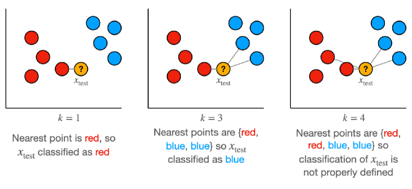
Figure 4: k-NN Classification. A simple solution for the last case is to randomly select one of the two classes or use an odd $k$ [50].

Three different algorithms are available to perform k-NN:

• Brute Force: here we simply calculate the distance from the point of interest to all the points in the training set and take the class with majority points.

• k-Dimensional Tree [51]: kd tree is a hierarchical binary tree. When this algorithm is used for k-NN classification, it rearranges the whole dataset in a binary tree structure, so that when test data is provided, it would give out the result by traversing through the tree, which takes less time than brute search.

• Ball Tree [52]: is a hierarchical data structure similar to kd trees and is particularly efficient for higher dimensions.

The hyperparameters selected for constructing our k-NN model are determined using GridSearchCV from the sklearn Python library [53]. This method identifies the optimal combination of hyperparameters from a predefined parameter grid based on a specified scoring function, with the negative mean squared error employed in our work. Additionally, GridSearchCV utilizes cross-validation to refine the model parameters, and in our case, a cv value of 10 was applied. The ultimate hyperparameters are as follows:

• the number of neighbors, the k value, is 4 when no feature selection is employed, 5 for feature selection with the Random Forest and Boruta, 6 when the feature selection is done with SHAP;

• the weight is the inverse of the distance used;

• the power parameter p for the Minkowski metric is 1, so we used the Manhattan distance.

• the algorithm hyperparameter used to compute the nearest neighbors was leaved to auto, so that the model will automatically use the most appropriate algorithm based on the values passed to the fit method.

IV.2.3 Random Forest

The third model utilized in our study is the Random Forest Regressor. This model works by creating an ensemble of Decision Trees during the training phase, each based on different subsets of input data samples. Within the construction of each tree, various combinations of features inherent in data patterns are incorporated into the decision-making process. By employing a sufficient number of trees (dependent on the problem space complexity and input data volume), the produced forest is likely to represent all given features [54]. Regression models, in general sense, are able to take variable inputs and predict an output from a continuous range. In the context of regression models, which predict an output within a continuous range, decision tree regressions typically lack the ability to produce continuous output. Instead, they are trained on examples with output lying in a continuous range.

The hyperparameters used to build our RFRegressor model were the following:

• the number of trees is 10000;

• the criterion to measure the quality of a split is the mean squared error;

• the maximum depth of the trees is set to None, so the nodes are expanded until all leaves are pure or until all leaves contain less than min_samples_split samples;

• the minimum number of samples required to split an internal node, the hyperparameter of the previous point min_samples_split, is set to 2;

• the number of feature to consider when looking for the best split hyperparameter is set to auto, so that the max features to consider is equal to the number of features available.

IV.2.4 Gradient Boosting

The fourth and last model used in our work is the Gradient Boosting Regressor. In the previous paragraph we talked about the bagging technique, here the technique is called boosting and is somehow complementary. Boosting is a sequential type of ensemble learning that uses the result of the previous model as input for the next one. Instead of training the models separately, the upgrade trains the models in sequence, each new model being trained to correct the errors of the previous ones. At each iteration the correctly predicted results are given a lower weight and those erroneously predicted a greater weight. It then uses a weighted average to produce a final result. Boosting is an iterative meta-algorithm that provides guidelines on how to connect a set of Weak Learners to create a Strong Learner. The key to the success of this paradigm lies in the iterative construction of Strong Learners, where each step involves introducing a Weak Learner tasked with ”adjusting the shot” based on the results obtained by its predecessors. Gradient Boosting employs standard Gradient Descent to minimize the loss function used in the process. Typically, the Weak Learners are decision trees, and in this case, the algorithm is termed gradient-boosted trees.

The typical steps of a Gradient Boosting algorithm are the following:

1. The average of the target values is calculated for the initial predictions and the corresponding initial residual errors.

2. A model (shallow decision tree) is trained with independent variables and residual errors as data to obtain predictions.

3. The additive predictions and residual errors are calculated with a certain learning rate from the previous output predictions obtained from the model.

4. Steps 2 and 3 are repeated a number M of times until the required number of models are built.

5. The final boost prediction is the additive sum of all previous made by the models.

The hyperparameters used to build our GBRegressor were the following:

• the loss function used is the squared error;

• the learning rate, which defines the contribution of each tree, is set to 0.01;

• the number of boosting stages is set to 10000;

• the function used to measure the quality of a split is the friedman_mse, or the mean squared error with the improvement by Friedman;

• the minimum number of samples required to split an internal node is set to 2;

• the maximum depth of the trees is set to None, so the nodes are expanded until all leaves are pure or until all leaves contain less than min_samples_split samples;

• the number of feature to consider when looking for the best split hyperparameter is set to None, so that the max features to consider is equal to the number of features available.

V Sampling techniques

This section introduces the techniques used in our work to perform cosmological parameters inference using the Pantheon+SH0ES type Ia Supernovae dataset. As we said, the methods used in our project are Markov Chain Monte Carlo (MCMC) and Nested Sampling. MCMC is a probabilistic method that explores the parameter space by generating a sequence of samples, where each sample is a set of parameter values. The core of the method is related to the Markov property, which means that the next state in the sequence depends only on the current state [55]. In the context of cosmological parameter inference, MCMC is often used to sample the posterior distribution of parameters given observational data. It explores the parameter space by creating a chain of samples, with the density of samples reflecting the posterior distribution. Through analysis of this chain, one can estimate the most probable values and uncertainties for cosmological parameters. In our work, we used two versions of Nested Sampling: the standard and the dynamic version, which is a slight variation of the former. Nested Sampling is a technique used for Bayesian evidence calculation and parameter estimation and involves enclosing a shrinking region of high likelihood within the prior space and iteratively sampling points from this region. Nested Sampling was developed to estimate the marginal likelihood, but it can also be used to generate posterior samples, and it can potentially work on harder problems where standard MCMC methods may get stuck. Dynamic Nested Sampling is an extension of Nested Sampling that adapts the sampling strategy during the process. It starts with a high likelihood region and dynamically adjusts the sampling to focus on regions of interest. This method is advantageous for exploring complex and multimodal parameter spaces, which can occur in cosmological models. At the end of each technique, we evaluated its performance by calculating the Bayesian Information Criterion [56] (BIC) and the Akaike Information Criterion [57] (AIC).

V.1 Markov Chain Monte Carlo (MCMC)

The Bayesian perspective on parameter estimation views probability as a measure of belief, treating parameters as random variables influenced by the available data and our prior beliefs. Essentially, with a predetermined prior parameter distribution, the data serves to adjust and refine our initial beliefs. This iterative process results in a posterior parameter distribution, consolidating all knowledge gained from the data. The posterior distribution encapsulates comprehensive information about the parameters, incorporating both the prior beliefs and the evidence provided by the data [58].

The posterior distribution can be derived from the likelihood and the prior using the Bayes theorem:

$$P(\Theta|D)=\frac{P(D|\Theta)\cdot\pi(\Theta)}{P(D)}=\frac{P(D|\Theta)\cdot\pi(\Theta)}{\int P(D|\Theta)\cdot\pi(\Theta)\,d\Theta}.$$ (27)

Due to the fact that the integral can be difficult to evaluate and that, in general, it is not necessary to know the exact posterior, the following approximation which provides the same shape information is used in most applications:

$$P(\Theta|D)\propto P(D|\Theta)\cdot\pi(\Theta).$$ (28)

The primary challenge in Bayesian parameter estimation lies in the general inability to derive the posterior distribution analytically, and even numerical analysis is often impractical. This longstanding issue found an ingenious solution through Markov Chain Monte Carlo (MCMC) sampling, representing a significant breakthrough in 20th-century statistics. MCMC produces a sequence of parameter sets (Markov chain) whose empirical distribution, over extended sequences, approximates or converges to the posterior distribution.

Markov Chain Monte Carlo sampling offers an elegant solution for evaluating model parameters, particularly when the corresponding posterior distribution cannot be accessed analytically. It generates a parameter sample, and as the sequence lengthens, its empirical distribution converges to the true posterior distribution. Consequently, any inquiry about the posterior parameter distribution can theoretically be addressed by examining the corresponding Markov chain.

Monte Carlo approaches aim to approximate a target density $p(x)$ where $x\in X$ (with $X$ as a high-dimensional space) by generating an independent and identically distributed set of samples ${\{x^{(i)}\}_{i=1}^{N}}$. This set of samples becomes instrumental in estimating integrals or maxima of the target function. While straightforward sampling routines exist for simple forms of $p(x)$, more sophisticated techniques like Markov Chain Monte Carlo sampling are necessary for most real-world applications.

Model	$H_{0}$		$\Omega_{m}$		$w$
	Mean	Std	Mean	Std	Mean	Std
$\Lambda$CDM	70.0	0.1	0.3	0.05	-1.0	0.1
	$H_{0}$		$\Omega_{m}$		$w_{0}$		$w_{z}$
	Mean	Std	Mean	Std	Mean	Std	Mean	Std
Linear Redshift	70.0	0.1	0.3	0.05	-1.0	0.1	-0.1	0.1
	$H_{0}$		$\Omega_{m}$		$w_{0}$		$w_{a}$
	Mean	Std	Mean	Std	Mean	Std	Mean	Std
CPL	70.0	0.1	0.3	0.05	-1.0	0.1	-0.5	0.1
	$H_{0}$		$\Omega_{m}$		$w_{0}$		$w_{a}$
	Mean	Std	Mean	Std	Mean	Std	Mean	Std
Squared Redshift	70.0	0.1	0.3	0.05	-1.0	0.1	-0.1	0.1
	$H_{0}$		$\Omega_{m}$		$b$		$\alpha$
	Mean	Std	Mean	Std	Mean	Std	Mean	Std
Generalized CG	70.0	0.1	0.3	0.05	-1.0	0.1	0.2	0.1
	$H_{0}$		$\Omega_{m}$		$b$		$b_{s}$		$\alpha$
	Mean	Std	Mean	Std	Mean	Std	Mean	Std	Mean	Std
Modified CG	70.0	0.1	0.3	0.05	-1.0	0.1	0	0.1	0.2	0.1

Table 1: Initial conditions for MCMC.

V.1.1 Markov chains

A Markov chain is a stochastic process which yields a sequence of states where one state depends only on the directly preceding one (the so-called Markov property):

$$P(x^{(i)}|x^{(i-1)},...,x^{(1)})=P(x^{(i)}|x^{(i-1)}).$$ (29)

Possible transitions between the states are specified by a transition matrix

$$T(x^{(i)}|x^{(i-1)})\quad\text{with}\quad\sum_{x^{(i)}}T(x^{(i)}|x^{(i-1)})=1\quad\forall i.$$ (30)

If $T\mathrel{\ensurestackMath{\stackon[1pt]{=}{\scriptscriptstyle\Delta}}}T(x^{(i)}|x^{(i-1)})$, the Markov chain is termed homogeneous. An invariant distribution $p(x)$ is one where the transition matrix is designed in a way that, after several steps and from any initial state, the chain converges to this distribution. This behavior aligns with the objectives when utilizing Markov Chain Monte Carlo (MCMC) sampling to approximate a posterior distribution that cannot be evaluated by other means. Achieving an invariant distribution necessitates constructing a stochastic, homogeneous transition matrix $T$ that is both irreducible and aperiodic. Irreducibility ensures that every state can be reached from any other state at some point, while aperiodicity guarantees that the chain avoids getting trapped in cycles. The detailed balance condition, or reversibility, serves as a sufficient but not necessary condition for the invariance of a target distribution $p(x)$:

$$p(x^{(i)})T(x^{(i-1)}|x^{(i)})=p(x^{(i-1)})T(x^{(i)}|x^{(i-1)}).$$ (31)

Thus, by ensuring detailed balance, it is possible to ensure that a target distribution $p(x)$ is invariant.

V.1.2 The Metropolis-Hastings (M-H) algorithm

The simplest and most commonly used MCMC algorithm is the M-H method [59, 60, 61, 62]. The iterative procedure is the following:

1. given a position $X(t)$ sample a proposal position $Y$ from the transition distribution $Q(Y;X(t))$;

2. accept this proposal with probability

   $$min\left(1,\frac{p(X|D)}{p(X(t)|D)}\frac{Q(X(t);Y)}{Q(Y;X(t))}\right),$$ (32)

where $D$ is a set of observations. The transition distribution $Q(Y;X(t))$ is an easy to sample probability distribution for the proposal $Y$ given a position $X(t)$. A common parameterization of $Q(Y;X(t))$ is a multivariate Gaussian distribution centered on $X(t)$ with a general covariance tensor that has been tuned for performance. It is worth emphasizing that if this step is accepted $X(t+1)=Y$; otherwise, the new position is set to the previous one $X(t+1)=X(t)$.

The Metropolis-Hastings (M-H) algorithm converges, as the number of iterations $t$ approaches infinity, to a stationary set of samples from the distribution. However, alternative algorithms exist, offering faster convergence rates and varying levels of implementation complexity.

V.1.3 The stretch move

This affine-invariant sampling algorithm informally called the ”stretch move”, was proposed by Goodman and Weare [63] and significantly outperforms standard M-H methods producing independent samples with a much shorter autocorrelation time. This method involves simultaneously evolving an ensemble of K walkers $S=\{X_{k}\}$ where the proposal distribution for one walker $k$ is based on the current positions of the $K-1$ walkers in the complementary ensemble $S_{[k]}=\{X_{j},\forall j\neq k\}$. Here, the term ”positions”, refers to a vector in the $N$-dimensional, real-valued parameter space.

To update the position of a walker at position $X_{k}$, a walker $X_{j}$ is drawn randomly from the remaining walkers $S_{[k]}$ and a new position is proposed:

$$X_{k}(t)\rightarrow Y=X_{j}+Z[X_{k}(t)-X_{j}],$$ (33)

where $Z$ is a random variable drawn from a distribution $g(Z=z)$. It is clear that if $g$ satisfies

$$g(z^{-1})=zg(z),$$ (34)

the proposal of (33) is symmetric. In this case, the chain will satisfy detailed balance if the proposal is accepted with probability

$$q=min\left(1,Z^{N-1}\frac{p(Y)}{p(X_{k}(t))}\right),$$ (35)

where $N$ is the dimension of the parameter space. Goodman and Weare [63] choose a particular form of $g(z)$:

$$g(z)\propto\begin{cases}\frac{1}{\sqrt{z}}&\text{if }z\in\left[\frac{1}{a},a\right],\\ 0&\text{otherwise}\end{cases}$$ (36)

where $a$ is an adjustable scale parameter that they set to 2.

V.1.4 Our implementation of Markov Chain Monte Carlo

In our work, we applied Markov Chain Monte Carlo (MCMC) to both the original dataset, which includes measured redshifts and distance modulus, and the predicted dataset, which includes measured redshift and predicted distance modulus obtained from our ensemble learning model. The hyperparameters used in our analysis are as follows:

• The number of walkers is set to 100.

• The move is the previously discussed StretchMove.

• The number of steps varies depending on the original and predicted dataset, with 1000 steps for the former and 2500 steps for the latter.

• The number of initial steps of each chain discarded as burn-in is set to 100.

• The initial positions of the walkers are randomly generated around the initial values for the cosmological parameters investigated with specified standard deviations (See Table 1).

V.2 Nested Sampling

Much of modern astronomy rests on making inferences about underlying physical models from observational data. In parallel, the amount of computational power to process these data also increased enormously. These changes opened up an entire new avenue for astronomers to try and learn about the universe using more complex models to answer increasingly sophisticated questions over large datasets. As a result, the standard statistical inference frameworks used in astronomy have generally shifted away from Frequentist methods such as maximum-likelihood estimation [64] (MLE) to Bayesian approaches to estimate the distribution of possible parameters for a given model that are consistent with the data and our current astrophysical knowledge.

The most popular method used in astronomy today is the previously discussed Markov Chain Monte Carlo (MCMC), which generates samples proportional to the posterior. While MCMC has had substantial success over the past few decades [65, 66], the most common implementations [67, 68, 69] tend to struggle when the posterior is comprised of widely-separated modes. In addition, because it only generates samples proportional to the posterior, it is difficult to use those samples to estimate the evidence to compare various models. Nested Sampling [70] is an alternative approach to posterior and evidence estimation that tries to resolve some of these issues. By generating samples in nested (possibly disjoint) “shells” of increasing likelihood, it is able to estimate the evidence $\mathcal{Z}_{M}$ for distributions that are challenging for many MCMC methods to sample from. The final set of samples can also be combined with their associated importance weights $p_{i}$ to generate associated estimates of the posterior.

The motivation behind nested sampling arises from the inherent challenge of directly sampling from the posterior distribution $P(\Theta)$. While methods like Markov Chain Monte Carlo (MCMC) aim to tackle this directly, nested sampling adopts a different strategy. Instead of directly addressing the complexity of this problem, nested sampling decomposes it into simpler steps by:

1. The posterior is divided into multiple simpler distributions.

2. Samples are drawn from each of these distributions sequentially.

3. The results from each distribution are combined afterward.

In contrast to MCMC methods, which aim to estimate the posterior $P(\Theta)$, nested sampling focuses on estimating the evidence $\mathcal{Z}$:

$$\mathcal{Z}=\int_{\Omega_{\Theta}}P(\Theta)d\Theta=\int_{\Omega_{\Theta}}\mathcal{L}(\Theta)\pi(\Theta)d\Theta.$$ (37)

Since this integral spans the entire multidimensional domain of $\Theta$ and is challenging to estimate, nested sampling redefines it as an integral over the prior volume $X$ of the parameter space:

$$\mathcal{Z}=\int_{\Omega_{\Theta}}\mathcal{L}(\Theta)\pi(\Theta)d\Theta=\int_{0}^{1}\mathcal{L}(X)dX.$$ (38)

Here, $\mathcal{L}(X)$ defines iso-likelihood contours outlining the volume $X$, while the prior volume $X(\lambda)$ represents the fraction of the prior where the likelihood $\mathcal{L}(\Theta)\geq\lambda$. With the prior being normalized, $X(\lambda=0)=1$ and $X(\lambda=\inf)=0$, setting the integration limits for equation (38).

The figure illustrates the difference between MCMC methods and nested sampling, where MCMC generates samples directly from the posterior, whereas nested sampling breaks the posterior into nested slices, samples from each, and then combines them to reconstruct the original distribution with appropriate weights.

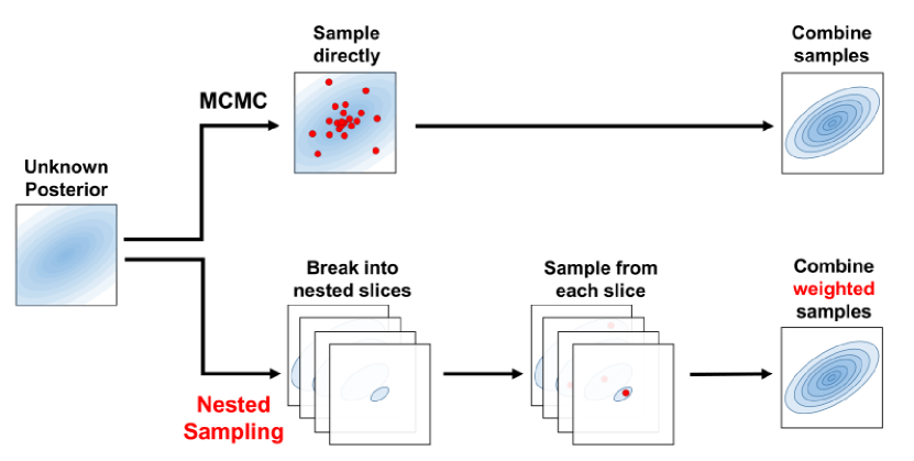
Figure 5: While MCMC methods attempt to generate samples directly from the posterior, Nested Sampling instead breaks up the posterior into many nested “slices”, generates samples from each of them, and then recombines the samples to reconstruct the original distribution using the appropriate weights [71].

V.2.1 Stopping criterion

Nested Sampling is primarily aimed at estimating evidence, with a commonly used stopping criterion [72, 73] being the termination of the sampling process when the set of dead points, and optionally the remaining live points, yields an integral that covers most of the posterior distribution. This termination condition, typically at iteration $i$, is expressed as:

$$\Delta\ln\hat{\mathcal{Z}}_{i}\equiv\ln\left(\hat{\mathcal{Z}}_{i}+\Delta\hat{\mathcal{Z}}_{i}\right)-\ln\hat{\mathcal{Z}}_{i}<\epsilon,$$ (39)

where $\Delta\hat{\mathcal{Z}}_{i}$ represents the estimated remaining evidence yet to be integrated, and $\epsilon$ is a user-defined tolerance. If the final set of live points is not included in the set of dead points, the default tolerance in the Python library dynesty [71, 74], is set to $\epsilon=10^{-2}$ (1% of the evidence remaining). If the final set of live points is included, a slightly more permissive tolerance is used: $\epsilon=10^{-3}(K-1)+10^{-2}$.

V.2.2 Evidence and Posterior

Once a final set of samples $\{\Theta_{1},\ldots,\Theta_{N}\}$ is obtained, the 1-D evidence integral can be estimated using standard numerical techniques. To ensure small approximation errors, dynesty employs the 2nd-order trapezoid rule:

$$\hat{\mathcal{Z}}=\sum_{i=1}^{N+K}\frac{1}{2}[\mathcal{L}(\Theta_{i-1})+\mathcal{L}(\Theta_{i})]\times(\hat{X}_{i-1}-\hat{X}_{i})\equiv\sum_{i=1}^{N+K}\hat{p}_{i},$$ (40)

where $X_{0}=X(\lambda=0)=1$ and $p_{i}\equiv[\mathcal{L}(\Theta_{i-1})+\mathcal{L}(\Theta_{i})]\times(\hat{X}_{i-1}-\hat{X}_{i})$ is the estimated importance weight. The posterior $P(\Theta)$ can also be estimated from the same set of $N+K$ dead points using the associated importance weights:

$$\hat{P}(\Theta)=\frac{\sum_{i=1}^{N+K}\hat{p}(\Theta_{i})\delta(\Theta_{i})}{\sum_{i=1}^{N+K}\hat{p}(\Theta_{i})}={\hat{\mathcal{Z}}^{-1}}\sum_{i=1}^{N+K}\hat{p}(\Theta_{i})\delta(\Theta_{i}).$$ (41)

By default, dynesty computes this posterior estimate using the mean values of $\hat{X}_{i}$.

V.2.3 Benefits and drawbacks of Nested Sampling

Because of its alternative approach to sampling from the posterior, Nested Sampling offers several advantages over traditional MCMC approaches:

1. Nested Sampling can estimate both the evidence $\mathcal{Z}$ and the posterior $P(\Theta)$. In contrast, MCMC methods typically only constrain the posterior [75, 76].

2. Nested Sampling is effective at sampling from multimodal distributions, a challenge for many MCMC methods.

3. Nested Sampling employs well-motivated stopping criteria focused on power estimation, whereas MCMC stopping criteria based on effective sample sizes can feel arbitrary.

4. Unlike MCMC methods, which require convergence to the posterior before generating valid samples [77, 78], Nested Sampling smoothly integrates over the posterior starting from the prior.

However, Nested Sampling also has drawbacks. Unlike MCMC, which focuses on directly sampling the posterior, Nested Sampling primarily estimates the evidence $\mathcal{Z}$, with the posterior as a by-product. This approach has limitations:

1. Nested Sampling implementations often sample from uniform distributions, limiting flexibility for general distributions. Deriving appropriate prior transforms, especially for complex priors, can be challenging.

2. The runtime of Nested Sampling increases with the size of the prior volume to be integrated over. Larger priors require sampling in extended tails for evidence estimation, even if the posterior remains largely unchanged.

3. Nested Sampling’s integration rate ($\Delta\ln X$) remains constant regardless of the position in the distribution. Increasing the number of live points improves accuracy for both posterior and evidence estimation without allowing prioritization between them.

V.2.4 Bounding Distributions

In a general sense, dynesty aims to utilize the distribution of current live points to gain an approximate understanding of the shape and size of different regions within the previous volume being sampled. This information guides various sampling methods to enhance overall efficiency.

In our approach, known as the multiple ellipsoids method, the first step involves creating a bounding ellipsoid that encompasses all live points. Subsequently, 2 k-means clusters are initialized at the endpoints of the principal axes. The positions of these clusters are optimized, and live points are assigned to each cluster. New pairs of bounding ellipsoids are then constructed for each new cluster of live points. This decomposition process iterates until further decomposition is not accepted.

V.2.5 Sampling Methods

After constructing a bounds distribution, dynesty proceeds to generate samples conditioned on those bounds. This process can be summarized by the equation $f(sC_{b},\Theta)\rightarrow\Theta^{\prime}$, where $C_{b}$ represents the covariance associated with a particular bound, $\Theta$ is the initial position, $\Theta^{\prime}$ is the proposed final position, and $s\sim 1$ is a scale factor adaptively adjusted during the run to achieve optimal acceptance rates. We utilized a uniform sampling method in our work.

This procedure, which inherently produces independent samples between iterations, performs best when the volume of the bounds closely matches the current prior volume, resulting in approximately 10% acceptance rates.

The general procedure for generating uniform samples from overlapping bounds is as follows [79]:

1. Randomly select a bound $b$ with probability $p_{b}\propto X_{b}$, where $X_{b}$ represents the volume of the bound.

2. Sample a point $\Theta_{b}$ uniformly from the bound.

3. Accept the point with probability $1/q$, where $q\geq 1$ is the number of bounds $\Theta_{b}$ lies within.

This approach ensures that each proposed sample is drawn from the bounds distribution $B(\Theta)$, which is the union of all bounds and has a volume $X_{B}\leq\sum_{b=1}^{N_{b}}X_{b}$, strictly less than or equal to the sum of the volumes of each individual bound.

V.3 Dynamic Nested Sampling

Previously, in section V.2.3, we outlined three main limitations of basic Nested Sampling implementations:

1. They typically require a prior transform.

2. Their runtime is influenced by the size of the prior.

3. The rate of posterior integration remains constant.

While the first two limitations are inherent to Nested Sampling as a sampling strategy, the third one is not. The algorithm’s inability to ”prioritize” the estimation of either the evidence $\mathcal{Z}$ or the posterior $P(\Theta)$ stems from the constant number of live points $K$ throughout a run, thereby setting the integration rate $\Delta\ln X$. This results in what we refer to as Static Nested Sampling.

To tackle this issue, Higson et al. [74] proposed a straightforward modification: allowing the number of live points to vary during the run, termed Dynamic Nested Sampling. This modification enables a focus on sampling the posterior $P(\Theta)$, akin to MCMC approaches, while still retaining Nested Sampling’s advantages for estimating evidence $\mathcal{Z}$ and sampling from complex, multimodal distributions.

The crux of the Dynamic Nested Sampling algorithm lies in determining how the number of live points $K_{i}$ at a given iteration $i$ should vary. The objective is to have $K_{i}$ larger in regions where higher resolution is needed (resulting in a slower integration rate $\Delta\ln X_{i}$) and smaller in regions where faster traversal of the current prior volume is preferred.

Generally, the desired number of live points $K(X)$ as a function of prior volume $X$ should follow a specific importance function $I(X)$, often expressed as:

$$K(X)\propto I(X).$$ (42)

While the function $I(X)$ can be general, dynesty defaults to a function proposed by Higson et al. [74], which combines posterior and evidence importance:

$$I(X)=f^{P}I^{P}(X)+(1-f^{P})I^{\mathcal{Z}}(X),$$ (43)

where $f^{P}$ represents the relative importance assigned to estimating the posterior.

The posterior importance function $I^{P}(X)$ is defined as the probability density function (PDF) of the importance weight:

$$I^{P}(X)\equiv p(X).$$ (44)

This implies a preference for allocating more live points in regions with higher posterior mass.

The evidence importance function $I^{\mathcal{Z}}(X)$ is defined as:

$$I^{\mathcal{Z}}(X)\equiv\frac{1-{\mathcal{Z}(X)/\mathcal{Z}}}{\int_{0}^{1}(1-{\mathcal{Z}(X)/\mathcal{Z})dX}}.$$ (45)

This suggests allocating more live points when there is uncertainty in integrating over the posterior.

V.3.1 Our implementation of Static and Dynamic Nested sampling

As with the MCMC method, we applied Static and Dynamic Nested Sampling to both the original and predicted dataset. The hyperparameters used are the same for both the sampling methods and are the following:

• The number of live points varies depending on the original and predicted dataset, with 1000 steps for the former and 2500 steps for the latter.

• The bounding distribution used is the multi ellipsoids.

• The sampling method used is uniform.

• The maximum number of iterations, as the number of likelihood evaluations, is set to no limit. Iterations will stop when the termination condition is reached.

• The dlogz value, which sets the $\epsilon$ of the termination condition (39), is set to 0.01.

V.4 Information Criteria

Let us consider now two statistical criteria in order to compare our MCMC and Nested Sampling results:

• The Akaike Information Criterion (AIC), defined as

  $$AIC=-2\ln\mathcal{L}+2k,$$ (46)

  where $\mathcal{L}$ is the maximum likelihood and $k$ is the number of parameters in the model. The optimal model is the one that minimises the AIC, since it provides an estimate of a constant plus the relative difference between the unknown true likelihood function of the trained sampler and the fitted likelihood function of the cosmological model. Therefore, a lower AIC indicates that the model is closer to the true underlying likelihood.

• The Bayesian Information Criterion (BIC) defined as:

  $$BIC=-2\ln\mathcal{L}+k\ln N,$$ (47)

  where $N$ is the number of data points used in the fit. The BIC serves as an estimate of a function related to the posterior probability of a model being the true model within a Bayesian framework. Therefore, a lower BIC indicates that a model is deemed more likely to be the true model.

VI Results

As mentioned before, our work can be divided into two main sections: the first one, where we operate on the original SNe type Ia dataset; the second one, where we use the predicted distance modulus dataset after feature selection methods and an ensemble model. In particular, as discussed earlier, we used three feature selection methods to build the predicted dataset:

• Random Forest: here we have taken the 18 most important features out of the 70 total. The features considered are: m_b_corr, mB, zCMB, x0, zHEL, zHD, std_flux, m_b_corr_err_VPEC, MU_SH0ES_ERR_DIAG, m_b_corr_err_DIAG, skew, NDOF, percent_amplitude, DEC, biasCors_m_b_COVSCALE, fpr35, K, COV_c_x0.

• Boruta: here we have taken the confirmed features. The 13 accepted features employed are: m_b_corr, mB, x0, zCMB, zHEL, zHD, std_flux, m_b_corr_err_VPEC, MU_SH0ES_ERR_DIAG, m_b_corr_err_DIAG, percent_amplitude, DEC, MWEBV.

• SHAP: as with the Random Forest, also here we have taken the 18 most important features. The features selected are: m_b_corr, mB, zCMB, x0, zHEL, zHD, std_flux, m_b_corr_err_VPEC, MU_SH0ES_ERR_DIAG, m_b_corr_err_DIAG, percent_amplitude, DEC, NDOF, biasCors_m_b_COVSCALE, fpr35, skew, RA, COV_c_x0.

To summarise and highlight the differences between the three parameter spaces used, the figure below shows the Random Forest and SHAP importance, on a logarithmic scale, of the features selected by at least one of the techniques, together with the Boruta classification.

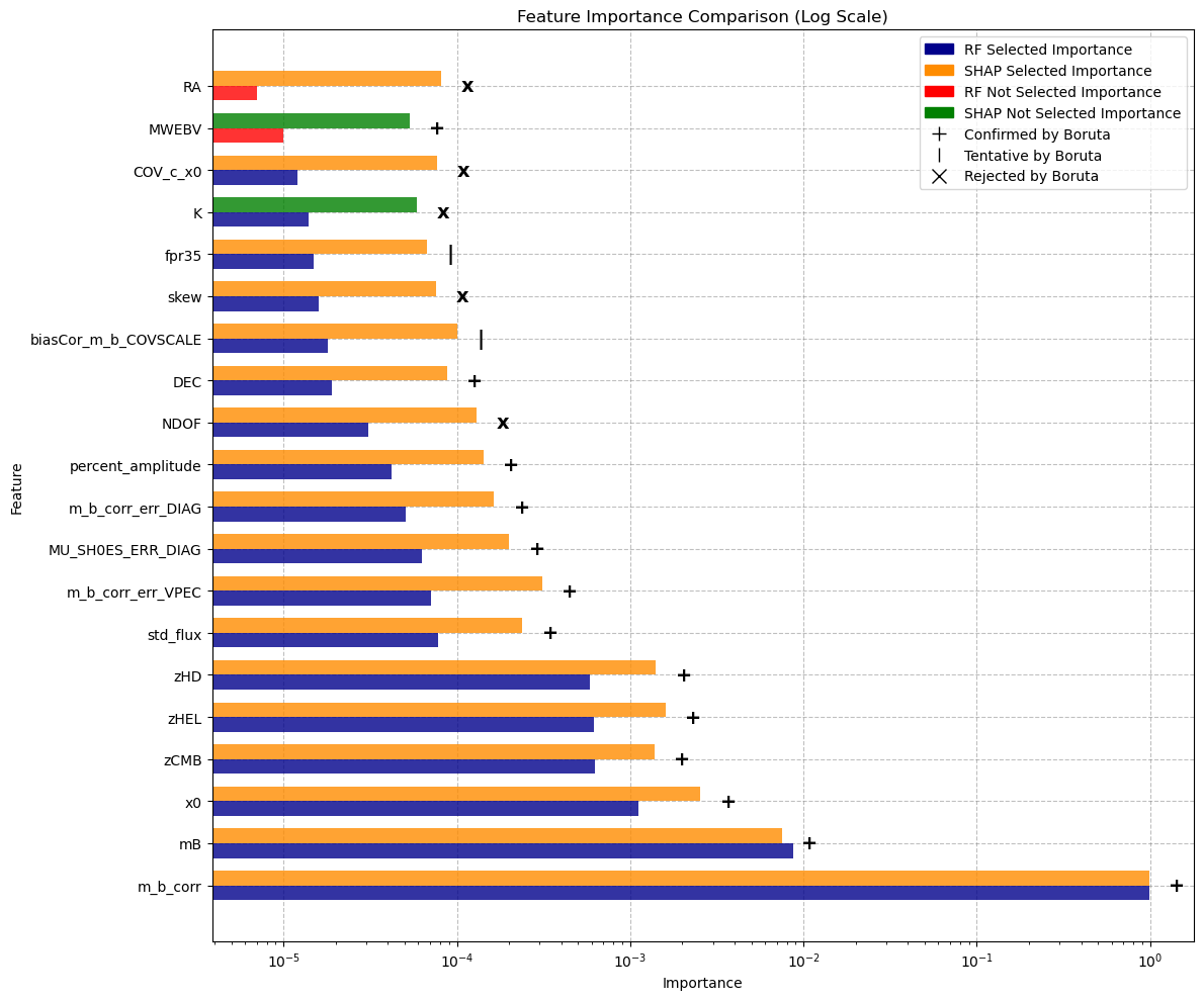
Figure 6: Feature Importance Comparison: The graph uses dark blue bars to show the importance of features selected by the RF model, while dark orange bars show the importance of features selected by SHAP. Red bars represent the importance of features not selected by the RF model, and green bars represent the importance of features not selected by SHAP. The symbols indicate the Boruta classification: $\mathbf{+}$ for confirmed, $\mathbf{|}$ for tentative, and $\mathbf{x}$ for rejected features. More information on all the features (Pantheon+SH0ES dataset and additions) can be found in the Appendix.

We also performed a ’base’ case study where all 70 features were used to predict distance moduli with an ensemble model. After each MCMC and Nested Sampling iteration, BIC and AIC have been computed. The final cosmological parameters and their uncertainties have been obtained as the mean of the three methods used. This work is developed for all the previously introduced six cosmological models, thanks to the Astropy Python package [80]. A summary of the results is provided in the Appendix. This includes corner plots obtained by each technique and a table showing the key results, such as BIC and AIC scores, for each method.

In the next plots we will indicate with ’OR’ the case of the original dataset, with ’ALL’ the case where no feature selection is done (i.e. all features are used), with ’RF’ the case where Random Forest is used as feature selection technique, with ’BOR’ the case where Boruta technique is used and with ’SHAP’ the case where SHAP is used as feature selection method. In addition,’MCMC’, ’SNS’ (Static Nested Sampling) and ’DNS’ (Dynamic Nested Sampling) indicate the different sampling techniques.

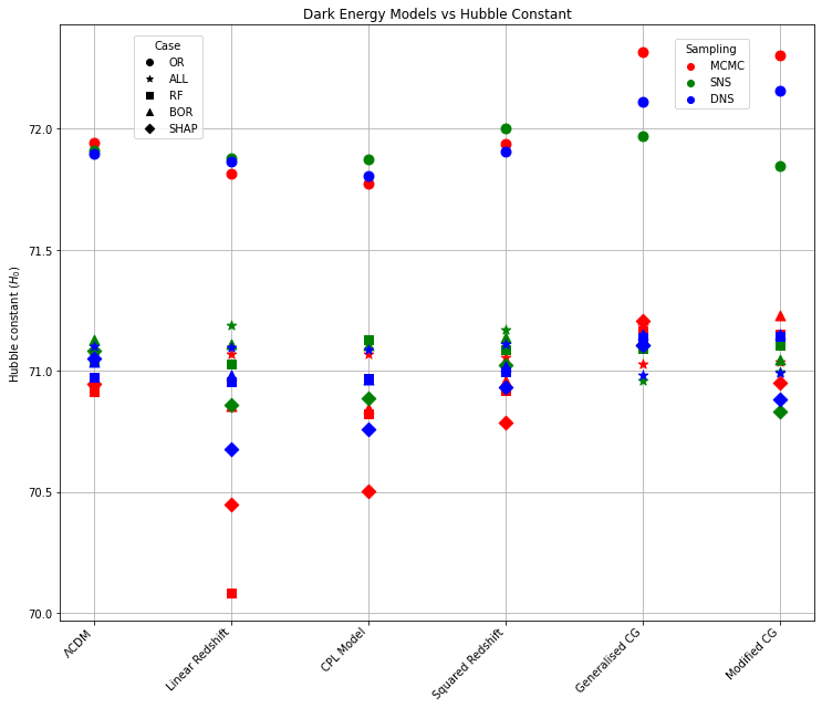
Figure 7: Hubble Constant Values.

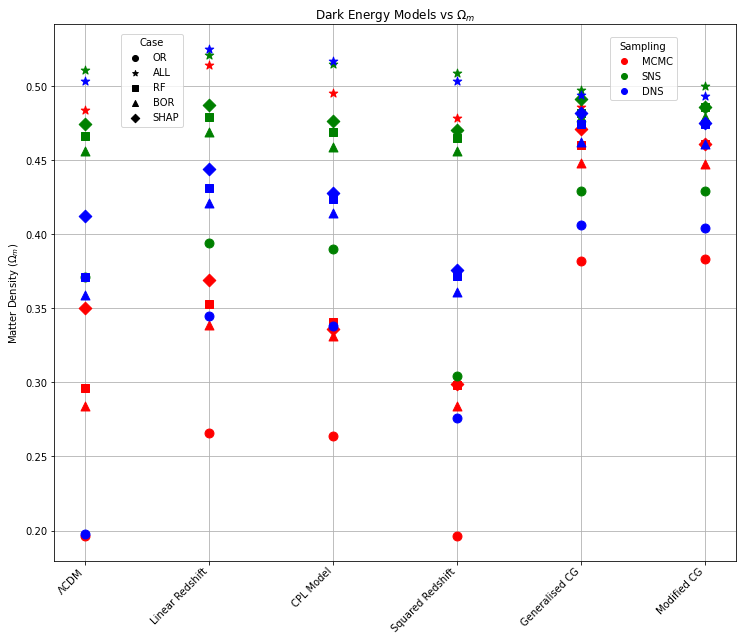
Figure 8: Matter Density Values.

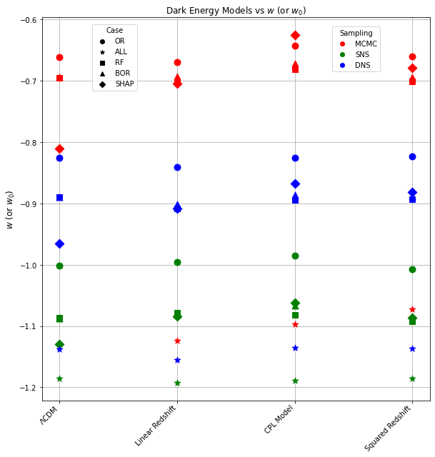
Figure 9: $w$ ($w_{0}$) Values.

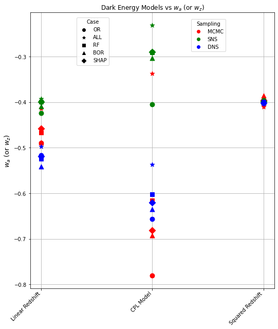
Figure 10: $w_{a}$ ($w_{z}$) Values.

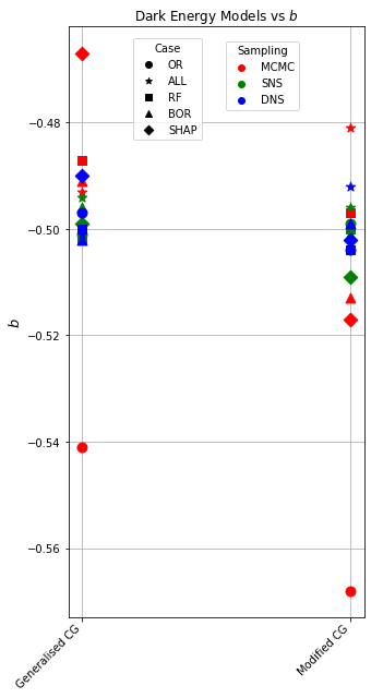
Figure 11: $b$ Values

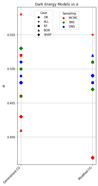
Figure 12: $\alpha$ Values

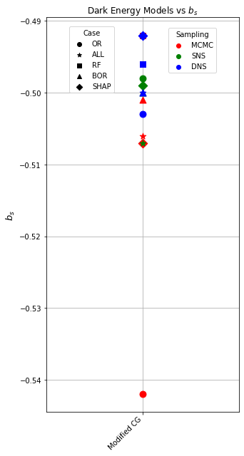
Figure 13: $b_{s}$ Values

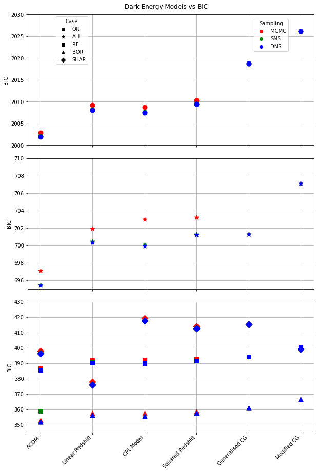
Figure 14: BIC Values.

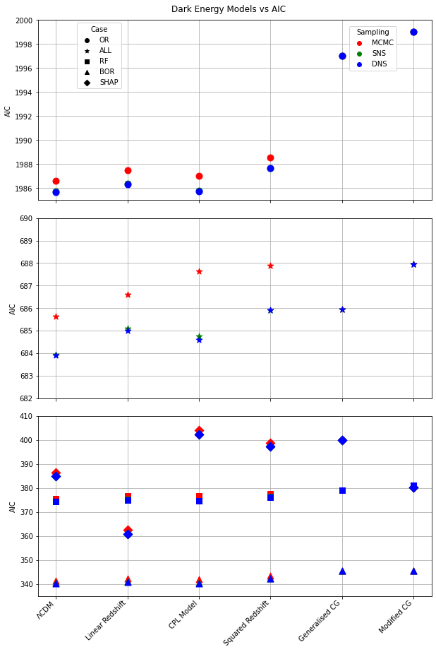
Figure 15: AIC Values.

Figure 7 shows how the values found in the first part of the study, from the original dataset, are significantly higher than the values found in the second part. The opposite trend is present in the Figure 8, but it is less clear. Interestingly, the GCG and MCG models have higher mean values for both parameters compared to all other models. In Figure 9, the values seem to be related to the particular sampling technique used, with an exception represented by the case where no feature selection has been applied, which is an alarming sign for its performance. Furthermore, in the Figure 10, a notable finding is how the Linear and Squared Redshift models present more or less the same results, while the CPL model covers a much wider range of values.

From the Figures 15 and 15, which show the values of BIC and AIC respectively for the analysed models, we can draw some interesting conclusions. Firstly, the values of BIC and AIC are much higher in the original dataset with respect to the other four cases, but this is due to the difference in the size of the dataset used, complete for the first scenario and 20% for the others, which leads to much larger penalty terms in the final values of the Information Criteria. Secondly, among the scenarios of the second part of the study, the case where no feature selection has been applied, has the highest values in BIC and AIC, which is representative of the fact that this is the worst case analysed, because not only we do not obtain a better performance, but we also have the higher complexity in the model. Among the three cases analysed, Boruta clearly has the lowest Information Criteria values and therefore the better sampling performance. Looking at the models, it is interesting to note that from the original dataset scenario to those where the feature selection has been applied, the Chaplygin Gas models have the greatest increase in performance compared to the other models. Finally, remaining in the three cases of feature selection, the model that has the lowest mean values of BIC and AIC is the Linear Redshift one, but this may be due to the low redshift of our dataset, which favours this model.

VII Discussion and Conclusions

In this work we have performed a test of six dark energy models with recent observations of Type Ia Supernovae. First, we tested each model by inferring its cosmological parameters by using Markov Chain Monte Carlo, Static Nested Sampling and Dynamic Nested Sampling. Secondly, we tried a different approach using machine learning. We built a regression model where the distance modulus of each supernova, the crucial data for inferring the cosmological parameters, was computed by the machine learning model, thanks to the other available features. In fact, we have not only relied on the features provided by the original dataset [81], but we have extended it by several features, bringing the total number to 74. The machine learning model used to compute the distance moduli is an ensemble model composed by four models: the MultiLayer Perceptron, the k-Nearest Neighbours, the Random Forest Regressor and the Gradient Boosting model. In order to improve the performance of our ensemble learning model, we applied different feature selection techniques, emphasising the importance of a data-driven approach. We have inferred the cosmological parameters of each model in four different cases: a case where no feature selection is applied (a sort of ’base’ case), a case where the first 18 features selected by the Random Forest are used to infer the distance moduli, a case where the feature selection method used is Boruta, and finally the case where the features used are the first 18 selected by SHAP. For every case, we repeated the process done in the first part of the study, or the use of MCMC and Nested Sampling, to infer the cosmological parameters for each model. By incorporating feature selection methods, we ensured that our models focused on the most relevant and informative features, thereby improving the robustness of the distance modulus predictions.

In the first phase of our study, the $\Lambda$CDM parameters were found to be consistent with established observations, confirming its status as a robust standard cosmological model. While the introduction of new parameters in the linear, squared redshift and CPL models led to slight deviations, the overall parameter values remained relatively similar across the different parameterisations. Instead, the Generalised and Modified Chaplygin Gas models showed significant deviations, especially in the matter density parameter, making them the worst performing of the six models.

Moving to the second part of our work, it is important to point out the results of the feature selection processes. The analysis shows that the most important feature by a significant margin is m_b_corr, which represents the Tripp1998 corrected/standardised $m_{b}$ magnitude. Following at some distance are mB (SALT2 uncorrected brightness, Guy et al. [82]) and x0 (SALT2 light curve amplitude). Next, in importance, are zCMB, zHEL and zHD, corresponding to the CMD corrected redshift, the heliocentric redshift and the Hubble diagram redshift respectively. While the remaining features are of lesser importance, their contributions are roughly comparable. It is worth noticing that the selected features are predominantly from the original dataset, with only a few additions made by us, such as std_flux, percent_amplitude, skew, fpr35, and K. This highlights the robustness of the original dataset features in influencing the predictive power of our models. However, the inclusion of additional features by us has provided valuable insights and contributed to the overall effectiveness of the feature selection process.

In the second section of our work, the first result we noticed is the clear difference in the performance of the ensemble model between the case where no feature selection is applied and the three cases where it is present. In the former, the parameters differ significantly from the values found in the first part of the work, but also the values of the information criteria, BIC and AIC, are almost two times the values of the cases where feature selection is applied. The performances observed for the three feature selection models are quite close, following a similar trend to the first part of the study. In particular, by looking at the values of the most important cosmological parameters, the Generalised and Modified Chaplygin Gas models appear to be slightly less effective than the other four models. Among Random Forest, Boruta and SHAP, the former seems to perform slightly worse, while the other two show comparable results. Furthermore, our analysis reveals an interesting aspect in the estimation of the $w_{a}$ (or $w_{z}$) parameter across the dark energy models. The Linear and Squared Redshift parameterisation models give similar estimates, while the CPL model shows a larger variation. In general, the trend across all six models indicates a slightly lower $H_{0}$ and a slightly higher $\Omega_{m}$ compared to the values obtained in the first part of the study. It is worth noting that Boruta stands out as the model with relatively lower information criteria values. It is interesting to note that when looking at the BIC and AIC values, the models that seemed to be by far the worst in the first part of the study, i.e. the Generalised and Modified Chaplygin Gas models, in the case where no feature selection is applied, the result is only confirmed for the Modified Chaplygin Gas, while the Generalised one is among the best models. Instead, for the three cases of feature selection, the opposite happens, with the Generalised model behaving similarly to the CPL and Squared Redshift models, while the Modified model performs better than all these three. In summary, the feature selection models, especially Boruta, show consistent performance with variations in $H_{0}$ and $\Omega_{m}$. The unexpected ranking of the information criteria between the models, which challenges conventional expectations based on theoretical considerations, adds an interesting dimension to the overall interpretation. This highlights the importance of a data-driven approach to cosmological studies, where feature selection can lead to more nuanced insights into dark energy models.

In the future, we aim to extend our investigation using the cosmological constraints provided by the Dark Energy Spectroscopic Instrument (DESI). The recent DESI Data Release 1 [83] provides robust measurements of Baryon Acoustic Oscillations (BAO) in several tracers, including galaxies, quasars, and Lyman-$\alpha$ forests, over a wide redshift range from 0.1 to 4.2. These measurements provide valuable insights into the expansion history of the Universe, and place stringent constraints on cosmological parameters. The implications of the DESI BAO measurements are of particular interest for the nature of dark energy. The DESI data, in combination with other cosmological probes such as the Planck measurements of the CMB and the Type Ia supernova datasets, may provide new perspectives on the EoS parameter of dark energy ($w$) and its possible time evolution ($w_{0}$ and $w_{a}$). The discrepancy between the DESI BAO data and the standard $\Lambda$CDM model, especially in the context of the dark energy EoS, opens up avenues for further investigation. By incorporating the DESI BAO measurements into our analysis framework, we expect to refine our understanding of the dark energy dynamics and its implications for the overall cosmic evolution. In addition, recent results [84] show that a $\sim$ 2$\sigma$ discrepancy with the Planck $\Lambda$CDM cosmology in the DESI Luminous Red Galaxy (LRG) data at $z_{\text{eff}}=0.51$ leads to an unexpectedly large $\Omega_{m}$ value, $\Omega_{m}=0.668^{+0.180}_{-0.169}$. This anomaly causes the preference for $w_{0}>-1$ in the DESI data when confronted with the $w_{0}w_{a}$CDM model. Independent analyses confirm this anomaly and show that DESI data allow $\Omega_{m}$ to vary on the order of $\sim$ 2$\sigma$ with increasing effective redshift in the $\Lambda$CDM model. Given the tension between LRG data at $z_{\text{eff}}=0.51$ and Type Ia supernovae at overlapping redshifts, it is expected that this anomaly will decrease in statistical significance with future DESI data releases, although an increasing $\Omega_{m}$ trend with effective redshift may persist at higher redshifts.

It is worth noticing that these results are not based on theoretical assumptions, but are derived directly from the data through our data-driven approach. By employing several feature selection techniques, we enable the data to guide our study of dark energy models.

In a forthcoming research, starting from the present results, we will use the information provided by DESI observations to develop more reliable constraints on dark energy models.

Appendix A Pantheon+SH0ES features

The total number of features provided by the dataset is 48 and are described in the Table A.

Table 2: Pantheon+SH0ES features

Feature	Description
CID	Candidate ID
IDSURVEY aaaaaaaaaa	Survey ID
zHD	Hubble Diagram Redshift (with CMB and VPEC corrections)
zHDERR	Hubble Diagram Redshift Uncertainty
zCMB	CMB Corrected Redshift
zCMBERR	CMB Corrected Redshift Uncertainty
zHEL	Heliocentric Redshift
zHELERR	Heliocentric Redshift Uncertainty
$m_{b}$_corr	Tripp1998 corrected/standardized $m_{b}$ magnitude
$m_{b}$_corr_err_DIAG	$m_{b}$ magnitude uncertainty from the diagonal covariance matrix
MU_SH0ES	Tripp1998 corrected/standardized distance modulus
MU_SH0ES_ERR_DIAG	Uncertainty on MU_SH0ES from the diagonal covariance matrix
CEPH_DIST	Cepheid calculated absolute distance to host (incorporated in the covariance matrix)
IS_CALIBRATOR	Binary indicator for SN in a host that has an associated cepheid distance
USED_IN_SH0ES_HF	1 if used in SH0ES 2021 Hubble Flow dataset, 0 if not included
$c$	SALT2 color
$c$ERR	SALT2 color uncertainty
$x_{1}$	SALT2 stretch
$x_{1}$ERR	SALT2 stretch uncertainty
$m_{B}$	SALT2 uncorrected brightness
$m_{B}$ERR	SALT2 uncorrected brightness uncertainty
$x_{0}$	SALT2 light curve amplitude
$x_{0}$ERR	SALT2 light curve amplitude uncertainty
COV_$x_{1}\_c$	SALT2 fit covariance between $x_{1}$ and $c$
COV_$x_{1}\_x_{0}$	SALT2 fit covariance between $x_{1}$ and $x_{0}$
COV_$c\_x_{0}$	SALT2 fit covariance between $c$ and $x_{0}$
RA	Right Ascension
DEC	Declination
HOST_RA	Host Galaxy RA
HOST_DEC	Host Galaxy DEC
HOST_ANGSEP	Angular separation between SN and host (arcsec)
VPEC	Peculiar velocity (km/s)
VPECERR	Peculiar velocity uncertainty (km/s)
MWEBV	Milky Way E(B-V)
HOST_LOGMASS	Host Galaxy Log Stellar Mass
HOST_LOGMASS_ERR	Host Galaxy Log Stellar Mass Uncertainty
PKMJD	Fit Peak Date
PKMJDERR	Fit Peak Date Uncertainty
NDOF	Number of degrees of freedom in SALT2 fit
FITCHI2	SALT2 fit chi squared
FITPROB	SNANA Fit probability
$m_{b}$_corr_err_RAW	Statistical only error on fitted $m_{B}$
$m_{b}$_corr_err_VPEC	VPECERR propagated into magnitude error
biasCor_$m_{b}$	Bias correction applied to brightness $m_{B}$
biasCorErr_$m_{b}$	Uncertainty on bias correction applied to brightness $m_{B}$
biasCor_$m_{b}$_COVSCALE	Reduction in uncertainty due to selection effects (multiplicative)
biasCor_$m_{b}$_COVADD	Uncertainty floor from intrinsic scatter model (quadrature)

Appendix B Additional features

In our work we added more features to those already present in the Pantheon+SH0ES dataset in order to gain more confidence in the upcoming results. The total number of features is 74, and here we present the ones we have added.

Amplitude (ampl)

The arithmetic average between the maximum and minimum magnitude:

$$ampl=\frac{mag_{max}-mag_{min}}{2}.$$ (48)

Beyond1std (b1std)

The fraction of photometric points above or under a certain standard deviation from the weighted average (by photometric errors):

$$b1std=P(|mag-\overline{mag}|>\sigma).$$ (49)

Flux Percentage Ratio (fpr)

The percentile is the value of a variable under which there is a certain percentage of light-curve data points. The flux percentile $F_{n,m}$ was defined as the difference between the flux values at percentiles $n$ and $m$. The following flux percentile ratios have been used:

$$fpr20 =F_{40,60}/F_{5,95},$$ (50)

$$fpr35 =F_{32.5,67.5}/F_{5,95},$$ (51)

$$fpr50 =F_{25,75}/F_{5,95},$$ (52)

$$fpr65 =F_{17.5,82.5}/F_{5,95},$$ (53)

$$fpr80 =F_{10,90}/F_{5,95}.$$ (54)

Lomb-Scargle Periodogram (ls)

The Lomb-Scargle periodogram [85, 86] is a method for finding periodic signals in irregularly sampled time series data. It handles irregularly spaced observations, calculates the power spectral density at different frequencies and uses least squares fitting. The statistic used in our work is the period given by the peak frequency of the Lomb-Scargle periodogram.

Linear Trend (slope)

The slope of the light curve in the linear fit, that is to say the $a$ parameter in the following linear relation:

$$mag=a\cdot t+b,$$ (55)

$$slope=a.$$ (56)

Median Absolute Deviation (mad)

The median of the deviation of fluxes from the median flux:

$$mad=median_{i}(|x_{i}-median_{j}(x_{j})|).$$ (57)

Median Buffer Range Percentage (mbrp)

The fraction of data points which are within 10 per cent of the median flux:

$$mbrp=P(|x_{i}-median_{j}(x_{j})|<0.1\cdot median_{j}(x_{j})).$$ (58)

Magnitude Ratio (mr)

An index used to estimate if the object spends most of the time above or below the median of magnitudes:

$$mr=P(mag>median(mag)).$$ (59)

Maximum Slope (ms)

The maximum difference obtained measuring magnitudes at successive epochs:

$$ms=max\left(\left|\frac{mag_{i+1}-mag_{i}}{t_{i+1}-t_{i}}\right|\right)=\frac{\Delta mag}{\Delta t}.$$ (60)

Percent Amplitude (pa)

The maximum percentage difference between maximum or minimum flux and the median:

$$pa=max(|x_{max}-median(X)|,|x_{min}-median(X)|).$$ (61)

Percent Difference Flux Percentile (pdfp)

The difference between the second and the 98th percentile flux, converted in magnitudes. It is calculated by the ratio $F_{5,95}$ on median flux:

$$pdfp=\frac{mag_{95}-mag_{5}}{median(mag)}.$$ (62)

Pair Slope Trend (pst)

The percentage of the last 30 couples of consecutive measures of fluxes that show a positive slope:

$$pst=P(x_{i+1}-x_{i}>0,i=n-30,\dots,n).$$ (63)

R Cor Bor (rcb)

The fraction of magnitudes that is below 1.5 mag with respect to the median:

$$rcb=P(mag>(median(mag)+1.5)).$$ (64)

Small Kurtosis (sk)

The kurtosis represents the departure of a distribution from normality and it is given by the ratio between the fourth-order momentum and the square of the variance. For small kurtosis, it is intended the reliable kurtosis on a small number of epochs:

$$sk=\frac{\mu_{4}}{\sigma^{2}}.$$ (65)

Skew (skew)

The skewness is an index of the asymmetry of a distribution. It is given by the ratio between the third-order momentum and the variance to the third power:

$$skew=\frac{\mu_{3}}{\sigma^{3}}.$$ (66)

Standard deviation (std)

The standard deviation of the fluxes.

Range of a Cumulative Sum ($R_{\text{cs}}$)

The range of a cumulative sum defined as:

$$R_{cs}=max(S)-min(S)$$ (67)

$$S=\frac{1}{N\sigma}\sum_{i=1}^{l}(mag_{i}-\overline{mag}).$$ (68)

Where $l=1,2,\dots,N$.

Stetson K (K)

A robust kurtosis measure [87] defined as:

$$\delta_{i}=\sqrt{\frac{N}{N-1}}\frac{mag_{i}-\overline{mag}}{mag\_err_{i}},$$ (69)

$$K=\frac{1/N\sum_{i=1}^{N}|\delta_{i}|}{\sqrt{1/N\sum_{i=1}^{N}\delta_{i}^{2}}}.$$ (70)

${Q_{3-1}}$

The difference between the third and first quartile of the magnitude.

Mean Variance (mvar)

This is a simple variability index defined as:

$$mvar=\frac{\sigma}{\overline{mag}}.$$ (71)

CAR features ($\sigma_{C},\tau,\text{mean}$)

To model irregularly sampled time series, the Continuous AutoRegressive (CAR) process, as presented in Brockwell and Davis [88] and Falk et al. [89], is employed. This continuous-time auto-regressive model involves three parameters and offers a natural and consistent means to estimate the characteristic time scale and variance of light curves. The CAR process is defined by the stochastic differential equation:

$$dX(t)=-\frac{1}{\tau}X(t)dt+\sigma_{C}\sqrt{dt}\epsilon(t)+bdt,$$ (72)

where ($\tau,\sigma_{C},t\geq 0$). The mean value of the light curve $X(t)$ is $b\tau$, and the variance is $\tau\sigma_{C}^{2}/2$. Here, $\tau$ is the relaxation time, interpreting the variability amplitude of the time series, and $\sigma_{C}$ describes variability on time scales shorter than $\tau$. $\epsilon(t)$ is a white noise process with zero mean and unit variance.

The likelihood function for such a CAR model, considering light-curve observations $\{x_{1},\ldots,x_{n}\}$ at times $\{t_{1},\ldots,t_{n}\}$ with measurement error variances $\{\delta_{1}^{2},\ldots,\delta_{n}^{2}\}$, is given by:

$$p(x|b,\sigma_{C},\tau)=\prod_{i=1}^{n}\frac{1}{\sqrt{2\pi(\Omega_{i}+\delta_{i}^{2})}}\exp\left\{-\frac{1}{2}\frac{(\hat{x}_{i}-x_{i}^{*})^{2}}{\Omega_{i}+\delta_{i}^{2}}\right\},$$ (73)

where $x^{*}_{i}=x_{i}-b\tau$, $\hat{x}_{0}=0$, $\Omega_{0}=\tau\sigma_{C}^{2}/2$, and $x_{i}$ and $\Omega_{i}$ are given by:

$$\hat{x}_{i} =a_{i}\hat{x}_{i-1}+\frac{a_{i}\Omega_{i-1}}{\Omega_{i-1}+\delta_{i-1}^{2}}(x^{*}_{i-1}+\hat{x}_{i-1}),$$ (74)

$$\Omega_{i} =\Omega_{0}(1-a_{i}^{2})+a_{i}^{2}\Omega_{i-1}\left(1-\frac{\Omega_{i-1}}{\Omega_{i-1}+\delta_{i-1}^{2}}\right),$$

$$a_{i} =e^{-(t_{i}-t_{i-1})/\tau}.$$

The parameter optimization involves maximizing the likelihood with respect to $\sigma_{C}$ and $\tau$, and $b$ is determined as the mean magnitude of the light curve divided by $\tau$.

Appendix C Importance of XAI

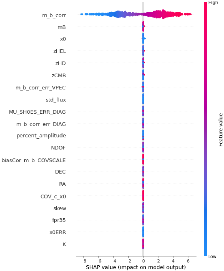
Figure 16: Beeswarm plot of the 20 most important features.

Explainable Artificial Intelligence (XAI) plays a crucial role in improving the interpretability of machine learning models, especially in scientific applications where transparency is essential. In this appendix, we highlight the importance of XAI using the SHAP framework and present a beeswarm plot (Figure 16) illustrating feature importances.

Explanatory AI methods such as SHAP provide insight into the decision-making process of complex models, fostering confidence and facilitating the identification of potential biases or errors. By quantifying the impact of each feature on model predictions, SHAP scores provide a comprehensive understanding of feature importance while maintaining desirable properties such as consistency and local accuracy.

To visually represent feature importance, we present a beeswarm plot showing the distribution of SHAP values for the 20 most important features. This plot provides an intuitive visualisation of the relative impact of different variables on the model’s predictions, facilitating the identification of key predictors and supporting informed decision making in scientific analyses.

Appendix D Additional Results

A summary of the results for the $\Lambda$CDM and CPL models is given for both the original dataset and the Boruta cases. For brevity, only the results for these specific models and cases are included in this section.

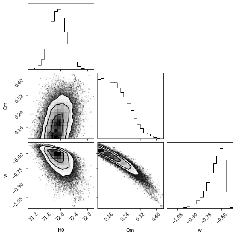
(a) MCMC

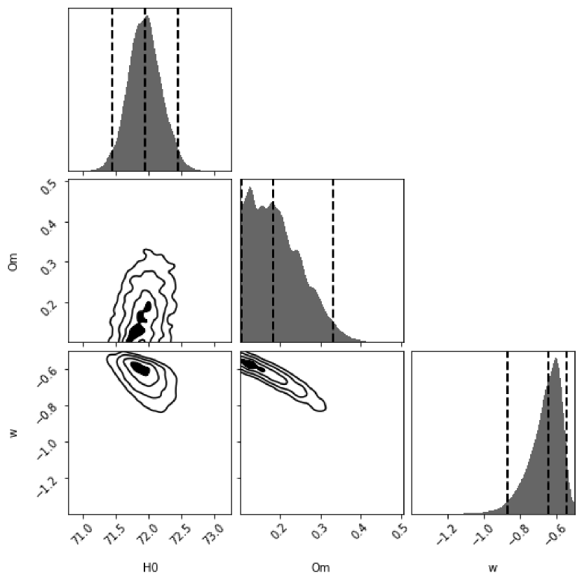
(b) SNS

(c) DNS

Figure 17: $\Lambda$CDM model corner plots for the original dataset.

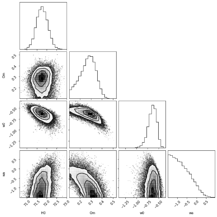
(a) MCMC

(b) SNS

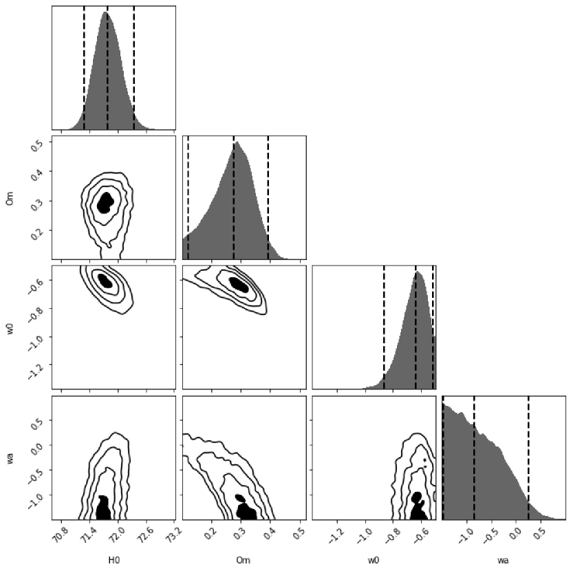
(c) DNS

Figure 18: CPL model corner plots for the original dataset.

(a) MCMC

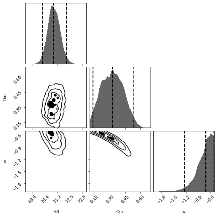
(b) SNS

(c) DNS

Figure 19: $\Lambda$CDM model corner plots with Boruta features.

(a) MCMC

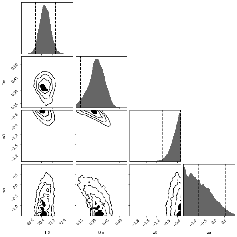
(b) SNS

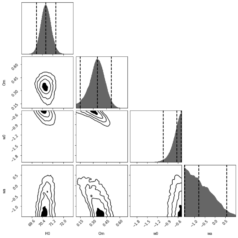
(c) DNS

Figure 20: CPL model with Boruta features.

Parameter	MCMC		SNS		DNS
	Mean	Std	Mean	Std	Mean	Std
$H_{0}$	71.944	0.249	71.909	4.701	71.899	3.409
$\Omega_{m}$	0.196	0.065	0.371	0.198	0.278	0.181
$w$	-0.661	0.094	-1.001	0.405	-0.826	0.352
BIC	2002.898		2002.014		2001.963
AIC	1986.581		1985.698		1985.646
Final Results
	Mean			Std
$H_{0}$	71.917			1.937
$\Omega_{m}$	0.281			0.092
$w$	-0.829			0.182

Table 3: $\Lambda$CDM model parameter values for the original dataset.

Parameter	MCMC		SNS		DNS
	Mean	Std	Mean	Std	Mean	Std
$H_{0}$	71.774	0.289	71.874	4.538	71.807	3.329
$\Omega_{m}$	0.264	0.071	0.390	0.183	0.338	0.150
$w_{0}$	-0.643	0.099	-0.985	0.405	-0.825	0.346
$w_{a}$	-0.781	0.489	-0.405	0.687	-0.656	0.649
BIC	2008.777		2007.535		2007.470
AIC	1987.021		1985.779		1985.714
Final Results
	Mean			Std
$H_{0}$	71.818			1.879
$\Omega_{m}$	0.331			0.082
$w_{0}$	-0.817			0.181
$w_{a}$	-0.614			0.355

Table 4: CPL model parameter values for the original dataset.

Parameter	MCMC		SNS		DNS
	Mean	Std	Mean	Std	Mean	Std
$H_{0}$	70.957	0.392	71.130	5.301	71.039	4.116
$\Omega_{m}$	0.284	0.107	0.456	0.192	0.359	0.191
$w$	-0.694	0.174	-1.088	0.417	-0.890	0.406
BIC	352.940		351.903		351.897
AIC	341.444		340.408		340.401
Final Results
	Mean			Std
$H_{0}$	71.042			3.270
$\Omega_{m}$	0.366			0.163
$w$	-0.890			0.332

Table 5: $\Lambda$CDM parameter values with Boruta features.

Parameter	MCMC		SNS		DNS
	Mean	Std	Mean	Std	Mean	Std
$H_{0}$	70.848	0.424	71.105	5.210	70.966	3.910
$\Omega_{m}$	0.331	0.101	0.459	0.185	0.414	0.154
$w_{0}$	-0.672	0.185	-1.067	0.415	-0.886	0.389
$w_{a}$	-0.693	0.585	-0.303	0.711	-0.635	0.720
BIC	357.482		355.805		355.618
AIC	342.154		340.478		340.291
Final Results
	Mean			Std
$H_{0}$	70.973			3.181
$\Omega_{m}$	0.401			0.147
$w_{0}$	-0.875			0.329
$w_{a}$	-0.544			0.672

Table 6: CPL parameter values with Boruta features.

References

- Perlmutter et al. [1999] S. Perlmutter, G. Aldering, G. Goldhaber, R. Knop, P. Nugent, P. G. Castro, S. Deustua, S. Fabbro, A. Goobar, D. E. Groom, et al., Measurements of and from 42 high-redshift supernovae, The Astrophysical Journal 517, 565 (1999).
- Schmidt et al. [1998] B. P. Schmidt, N. B. Suntzeff, M. Phillips, R. A. Schommer, A. Clocchiatti, R. P. Kirshner, P. Garnavich, P. Challis, B. Leibundgut, J. Spyromilio, et al., The high-Z supernova search: measuring cosmic deceleration and global curvature of the universe using type Ia supernovae, The Astrophysical Journal 507, 46 (1998).
- Peebles and Ratra [2003] P. J. E. Peebles and B. Ratra, The Cosmological Constant and Dark Energy, Rev. Mod. Phys. 75, 559 (2003), arXiv:astro-ph/0207347 .
- Bamba et al. [2012] K. Bamba, S. Capozziello, S. Nojiri, and S. D. Odintsov, Dark energy cosmology: the equivalent description via different theoretical models and cosmography tests, Astrophys. Space Sci. 342, 155 (2012), arXiv:1205.3421 [gr-qc] .
- Basilakos and Plionis [2009] S. Basilakos and M. Plionis, Is the Interacting Dark Matter Scenario an Alternative to Dark Energy ?, Astron. Astrophys. 507, 47 (2009), arXiv:0807.4590 [astro-ph] .
- Capozziello and De Laurentis [2011] S. Capozziello and M. De Laurentis, Extended Theories of Gravity, Phys. Rept. 509, 167 (2011), arXiv:1108.6266 [gr-qc] .
- Ostriker and Vishniac [1986] J. P. Ostriker and E. T. Vishniac, Generation of microwave background fluctuations from nonlinear perturbations at the era of galaxy formation, Astrophysical Journal, Part 2-Letters to the Editor (ISSN 0004-637X), July 15 306, L51 (1986).
- Weinberg [1989] S. Weinberg, The Cosmological Constant Problem, Rev. Mod. Phys. 61, 1 (1989).
- Geyer [1992] C. J. Geyer, Practical markov chain monte carlo, Statistical science , 473 (1992).
- Skilling [2004] J. Skilling, Nested sampling, in Aip conference proceedings, Vol. 735 (American Institute of Physics, 2004) pp. 395–405.
- Huterer and Turner [2001] D. Huterer and M. S. Turner, Probing dark energy: Methods and strategies, Physical Review D 64, 123527 (2001).
- Weller and Albrecht [2002] J. Weller and A. Albrecht, Future supernovae observations as a probe of dark energy, Physical Review D 65, 103512 (2002).
- Chevallier and Polarski [2001] M. Chevallier and D. Polarski, Accelerating universes with scaling dark matter, International Journal of Modern Physics D 10, 213 (2001).
- Linder [2008] E. V. Linder, The dynamics of quintessence, the quintessence of dynamics, General Relativity and Gravitation 40, 329 (2008).
- Barboza Jr and Alcaniz [2008] E. Barboza Jr and J. Alcaniz, A parametric model for dark energy, Physics Letters B 666, 415 (2008).
- Bento et al. [2002] M. Bento, O. Bertolami, and A. A. Sen, Generalized chaplygin gas, accelerated expansion, and dark-energy-matter unification, Physical Review D 66, 043507 (2002).
- Benaoum et al. [2012] H. B. Benaoum et al., Modified chaplygin gas cosmology, Advances in High Energy Physics 2012, 10.1155/2012/357802 (2012).
- D’Isanto et al. [2016] A. D’Isanto, S. Cavuoti, M. Brescia, C. Donalek, G. Longo, G. Riccio, and S. G. Djorgovski, An analysis of feature relevance in the classification of astronomical transients with machine learning methods, Monthly Notices of the Royal Astronomical Society 457, 3119 (2016).
- Nun et al. [2015] I. Nun, P. Protopapas, B. Sim, M. Zhu, R. Dave, N. Castro, and K. Pichara, Fats: Feature analysis for time series, arXiv preprint 10.48550/arXiv.1506.00010 (2015).
- Liaw and Wiener [2002] A. Liaw and M. Wiener, Classification and regression by randomforest, R News 2, 18 (2002).
- Kursa and Rudnicki [2011] M. B. Kursa and W. R. Rudnicki, The all relevant feature selection using random forest, arXiv preprint https://doi.org/10.48550/arXiv.1106.5112 (2011).
- Lundberg and Lee [2017] S. M. Lundberg and S.-I. Lee, A unified approach to interpreting model predictions, Advances in neural information processing systems 30, https://doi.org/10.48550/arXiv.1705.07874 (2017).
- Rumelhart et al. [1986] D. E. Rumelhart, G. E. Hinton, and R. J. Williams, Learning representations by back-propagating errors, nature 323, 533 (1986).
- Cover and Hart [1967] T. Cover and P. Hart, Nearest neighbor pattern classification, IEEE transactions on information theory 13, 21 (1967).
- Breiman [2001] L. Breiman, Random forests, Machine learning 45, 5 (2001).
- Schapire [1990] R. E. Schapire, The strength of weak learnability, Machine learning 5, 197 (1990).
- Quinlan [1986] J. R. Quinlan, Induction of decision trees, Machine learning 1, 81 (1986).
- Friedman [2001] J. H. Friedman, Greedy function approximation: a gradient boosting machine, Annals of statistics , 1189 (2001).
- Cai et al. [2016] Y.-F. Cai, S. Capozziello, M. De Laurentis, and E. N. Saridakis, f(T) teleparallel gravity and cosmology, Rept. Prog. Phys. 79, 106901 (2016), arXiv:1511.07586 [gr-qc] .
- Dunsby and Luongo [2016] P. K. Dunsby and O. Luongo, On the theory and applications of modern cosmography, International Journal of Geometric Methods in Modern Physics 13, 1630002 (2016).
- Demianski et al. [2012] M. Demianski, E. Piedipalumbo, C. Rubano, and P. Scudellaro, High redshift cosmography: new results and implication for dark energy, Mon. Not. Roy. Astron. Soc. 426, 1396 (2012), arXiv:1206.7046 [astro-ph.CO] .
- Capozziello et al. [2021] S. Capozziello, P. K. S. Dunsby, and O. Luongo, Model-independent reconstruction of cosmological accelerated–decelerated phase, Mon. Not. Roy. Astron. Soc. 509, 5399 (2021), arXiv:2106.15579 [astro-ph.CO] .
- Capozziello et al. [2020] S. Capozziello, R. D’Agostino, and O. Luongo, High-redshift cosmography: auxiliary variables versus Padé polynomials, Mon. Not. Roy. Astron. Soc. 494, 2576 (2020), arXiv:2003.09341 [astro-ph.CO] .
- Capozziello et al. [2018] S. Capozziello, R. D’Agostino, and O. Luongo, Cosmographic analysis with Chebyshev polynomials, Mon. Not. Roy. Astron. Soc. 476, 3924 (2018), arXiv:1712.04380 [astro-ph.CO] .
- Benetti and Capozziello [2019] M. Benetti and S. Capozziello, Connecting early and late epochs by f(z)CDM cosmography, JCAP 12, 008, arXiv:1910.09975 [astro-ph.CO] .
- Wang, Fa-Yin and Dai, Zi-Gao [2006] Wang, Fa-Yin and Dai, Zi-Gao, Constraining dark energy and cosmological transition redshift with type ia supernovae, Chinese Journal of Astronomy and Astrophysics 6, 561 (2006).
- Escamilla-Rivera and Capozziello [2019] C. Escamilla-Rivera and S. Capozziello, Unveiling cosmography from the dark energy equation of state, International Journal of Modern Physics D 28, 1950154 (2019).
- Cardone et al. [2004] V. F. Cardone, A. Troisi, and S. Capozziello, Unified dark energy models: A Phenomenological approach, Phys. Rev. D 69, 083517 (2004), arXiv:astro-ph/0402228 .
- Paul and Thakur [2013] B. Paul and P. Thakur, Observational constraints on modified chaplygin gas from cosmic growth, Journal of Cosmology and Astroparticle Physics 2013 (11), 052.
- Escamilla-Rivera et al. [2020] C. Escamilla-Rivera, M. A. C. Quintero, and S. Capozziello, A deep learning approach to cosmological dark energy models, Journal of Cosmology and Astroparticle Physics 2020 (03), 008.
- Yang et al. [2019] W. Yang, S. Pan, S. Vagnozzi, E. Di Valentino, D. F. Mota, and S. Capozziello, Dawn of the dark: unified dark sectors and the EDGES Cosmic Dawn 21-cm signal, JCAP 11, 044, arXiv:1907.05344 [astro-ph.CO] .
- Piedipalumbo et al. [2023] E. Piedipalumbo, S. Vignolo, P. Feola, and S. Capozziello, Interacting quintessence cosmology from Noether symmetries: Comparing theoretical predictions with observational data, Phys. Dark Univ. 42, 101274 (2023), arXiv:2307.02355 [gr-qc] .
- Lundberg et al. [2020] S. M. Lundberg, G. Erion, H. Chen, A. DeGrave, J. M. Prutkin, B. Nair, R. Katz, J. Himmelfarb, N. Bansal, and S.-I. Lee, From local explanations to global understanding with explainable ai for trees, Nature machine intelligence 2, 56 (2020).
- Li [2019] Q. Li, shap-shapley (2019), [Online; GitHub repository accessed December 20, 2023].
- Czerwinska [2020] U. Czerwinska, Push the limits of explainability — an ultimate guide to shap library (2020), [Online: Github Repository].
- Van Der Malsburg [1986] C. Van Der Malsburg, Frank rosenblatt: Principles of neurodynamics: Perceptrons and the theory of brain mechanisms, in Brain Theory: Proceedings of the First Trieste Meeting on Brain Theory, October 1–4, 1984 (Springer, 1986) pp. 245–248.
- Brescia et al. [2015] M. Brescia, S. Cavuoti, and G. Longo, Automated physical classification in the SDSS DR10. A catalogue of candidate quasars, Monthly Notices of the Royal Astronomical Society 450, 3893 (2015), arXiv:1504.03857 [astro-ph.GA] .
- Brescia et al. [2019] M. Brescia, M. Salvato, S. Cavuoti, T. T. Ananna, G. Riccio, S. M. LaMassa, C. M. Urry, and G. Longo, Photometric redshifts for X-ray-selected active galactic nuclei in the eROSITA era, Monthly Notices of the Royal Astronomical Society 489, 663 (2019), arXiv:1909.00606 [astro-ph.IM] .
- Kingma and Ba [2014] D. P. Kingma and J. Ba, Adam: A method for stochastic optimization, arXiv preprint https://doi.org/10.48550/arXiv.1412.6980 (2014).
- Nami [2021] Y. Nami, Why does increasing k decrease variance in knn? (2021), [Online; accessed December 20, 2023].
- Bentley [1975] J. L. Bentley, Multidimensional binary search trees used for associative searching, Communications of the ACM 18, 509 (1975).
- Bhatia et al. [2010] N. Bhatia et al., Survey of nearest neighbor techniques, arXiv preprint https://doi.org/10.48550/arXiv.1007.0085 (2010).
- Pedregosa et al. [2011] F. Pedregosa, G. Varoquaux, A. Gramfort, V. Michel, B. Thirion, O. Grisel, M. Blondel, P. Prettenhofer, R. Weiss, V. Dubourg, J. Vanderplas, A. Passos, D. Cournapeau, M. Brucher, M. Perrot, and E. Duchesnay, Scikit-learn: Machine learning in Python, Journal of Machine Learning Research 12, 2825 (2011).
- Hastie et al. [2009] T. Hastie, R. Tibshirani, J. Friedman, T. Hastie, R. Tibshirani, and J. Friedman, Overview of supervised learning, The elements of statistical learning: Data mining, inference, and prediction , 9 (2009).
- Norris [1998] J. R. Norris, Markov chains (Cambridge university press, 1998).
- Schwarz [1978] G. Schwarz, Estimating the dimension of a model, The annals of statistics , 461 (1978).
- Akaike [1974] H. Akaike, A new look at the statistical model identification, IEEE transactions on automatic control 19, 716 (1974).
- Bolstad [2009] W. M. Bolstad, Understanding computational Bayesian statistics, Vol. 644 (John Wiley & Sons, 2009).
- Metropolis et al. [1953] N. Metropolis, A. W. Rosenbluth, M. N. Rosenbluth, A. H. Teller, and E. Teller, Equation of state calculations by fast computing machines, The journal of chemical physics 21, 1087 (1953).
- MacKay [2003] D. J. MacKay, Information theory, inference and learning algorithms (Cambridge university press, 2003).
- Gregory [2005] P. Gregory, Bayesian logical data analysis for the physical sciences: a comparative approach with mathematica® support (Cambridge University Press, 2005).
- Hogg et al. [2010] D. W. Hogg, J. Bovy, and D. Lang, Data analysis recipes: Fitting a model to data, arXiv preprint https://doi.org/10.48550/arXiv.1008.4686 (2010).
- Goodman and Weare [2010] J. Goodman and J. Weare, Ensemble samplers with affine invariance, Comm. App. Math. Comp. Sci 5, 65 (2010).
- Fisher [1922] R. A. Fisher, On the mathematical foundations of theoretical statistics, Philosophical transactions of the Royal Society of London. Series A, containing papers of a mathematical or physical character 222, 309 (1922).
- Brooks et al. [2011] S. Brooks, A. Gelman, G. Jones, and X.-L. Meng, Handbook of markov chain monte carlo, ISSN (CRC press, 2011).
- Sharma [2017] S. Sharma, Markov chain monte carlo methods for bayesian data analysis in astronomy, Annual Review of Astronomy and Astrophysics 55, 213 (2017).
- Plummer et al. [2003] M. Plummer et al., JAGS: A program for analysis of Bayesian graphical models using Gibbs sampling, in Proceedings of the 3rd international workshop on distributed statistical computing, Vol. 124 (Vienna, Austria, 2003) pp. 1–10.
- Foreman-Mackey et al. [2013] D. Foreman-Mackey, D. W. Hogg, D. Lang, and J. Goodman, emcee: the mcmc hammer, Publications of the Astronomical Society of the Pacific 125, 306 (2013).
- Carpenter et al. [2017] B. Carpenter, A. Gelman, M. D. Hoffman, D. Lee, B. Goodrich, M. Betancourt, M. A. Brubaker, J. Guo, P. Li, and A. Riddell, Stan: A probabilistic programming language, Journal of statistical software 76, 10.18637/jss.v076.i01 (2017).
- Skilling [2006] J. Skilling, Nested sampling for general bayesian computation, Bayesian Analysis 1, 833 (2006).
- Speagle [2020] J. S. Speagle, DYNESTY: a dynamic nested sampling package for estimating Bayesian posteriors and evidences, Monthly Notices of the Royal Astronomical Society 493, 3132 (2020).
- Keeton [2011] C. R. Keeton, On statistical uncertainty in nested sampling, Monthly Notices of the Royal Astronomical Society 414, 1418 (2011).
- Higson et al. [2018] E. Higson, W. Handley, M. Hobson, and A. Lasenby, Sampling errors in nested sampling parameter estimation, Bayesian Analysis 13, 10.1214/17-ba1075 (2018).
- Higson et al. [2019] E. Higson, W. Handley, M. Hobson, and A. Lasenby, Dynamic nested sampling: an improved algorithm for parameter estimation and evidence calculation, Statistics and Computing 29, 891 (2019).
- Lartillot and Philippe [2006] N. Lartillot and H. Philippe, Computing bayes factors using thermodynamic integration, Systematic biology 55, 195 (2006).
- Heavens et al. [2017] A. Heavens, Y. Fantaye, A. Mootoovaloo, H. Eggers, Z. Hosenie, S. Kroon, and E. Sellentin, Marginal likelihoods from monte carlo markov chains, arXiv preprint https://doi.org/10.48550/arXiv.1704.03472 (2017).
- Gelman and Rubin [1992] A. Gelman and D. B. Rubin, Inference from iterative simulation using multiple sequences, Statistical science 7, 457 (1992).
- Vehtari et al. [2021] A. Vehtari, A. Gelman, D. Simpson, B. Carpenter, and P.-C. Bürkner, Rank-normalization, folding, and localization: An improved r for assessing convergence of mcmc (with discussion), Bayesian analysis 16, 667 (2021).
- Feroz and Hobson [2008] F. Feroz and M. P. Hobson, Multimodal nested sampling: an efficient and robust alternative to markov chain monte carlo methods for astronomical data analyses, Monthly Notices of the Royal Astronomical Society 384, 449 (2008).
- Price-Whelan et al. [2022] A. M. Price-Whelan, P. L. Lim, N. Earl, N. Starkman, L. Bradley, D. L. Shupe, A. A. Patil, L. Corrales, C. Brasseur, M. Nöthe, et al., The Astropy Project: sustaining and growing a community-oriented open-source project and the latest major release (v5. 0) of the core package, The Astrophysical Journal 935, 167 (2022).
- Scolnic et al. [2022] D. Scolnic, D. Brout, A. Carr, A. G. Riess, T. M. Davis, A. Dwomoh, D. O. Jones, N. Ali, P. Charvu, R. Chen, et al., The Pantheon+ analysis: the full data set and light-curve release, The Astrophysical Journal 938, 113 (2022).
- Guy et al. [2007] J. Guy, P. Astier, S. Baumont, D. Hardin, R. Pain, N. Regnault, S. Basa, R. Carlberg, A. Conley, S. Fabbro, et al., SALT2: using distant supernovae to improve the use of type Ia supernovae as distance indicators, Astronomy & Astrophysics 466, 11 (2007).
- DESI Collaboration et al. [2024] DESI Collaboration, A. G. Adame, J. Aguilar, S. Ahlen, S. Alam, D. M. Alexander, M. Alvarez, O. Alves, A. Anand, U. Andrade, E. Armengaud, S. Avila, A. Aviles, H. Awan, B. Bahr-Kalus, S. Bailey, C. Baltay, A. Bault, J. Behera, S. BenZvi, A. Bera, F. Beutler, D. Bianchi, C. Blake, R. Blum, S. Brieden, A. Brodzeller, D. Brooks, E. Buckley-Geer, E. Burtin, R. Calderon, R. Canning, A. Carnero Rosell, R. Cereskaite, J. L. Cervantes-Cota, S. Chabanier, E. Chaussidon, J. Chaves-Montero, S. Chen, X. Chen, T. Claybaugh, S. Cole, A. Cuceu, T. M. Davis, K. Dawson, A. de la Macorra, A. de Mattia, N. Deiosso, A. Dey, B. Dey, Z. Ding, P. Doel, J. Edelstein, S. Eftekharzadeh, D. J. Eisenstein, A. Elliott, P. Fagrelius, K. Fanning, S. Ferraro, J. Ereza, N. Findlay, B. Flaugher, A. Font-Ribera, D. Forero-Sánchez, J. E. Forero-Romero, C. S. Frenk, C. Garcia-Quintero, E. Gaztañaga, H. Gil-Marín, S. G. A. Gontcho, A. X. Gonzalez-Morales, V. Gonzalez-Perez, C. Gordon, D. Green, D. Gruen, R. Gsponer, G. Gutierrez, J. Guy, B. Hadzhiyska, C. Hahn, M. M. S. Hanif, H. K. Herrera-Alcantar, K. Honscheid, C. Howlett, D. Huterer, V. Iršič, M. Ishak, S. Juneau, N. G. Karaçaylı, R. Kehoe, S. Kent, D. Kirkby, A. Kremin, A. Krolewski, Y. Lai, T. W. Lan, M. Landriau, D. Lang, J. Lasker, J. M. Le Goff, L. Le Guillou, A. Leauthaud, M. E. Levi, T. S. Li, E. Linder, K. Lodha, C. Magneville, M. Manera, D. Margala, P. Martini, M. Maus, P. McDonald, L. Medina-Varela, A. Meisner, J. Mena-Fernández, R. Miquel, J. Moon, S. Moore, J. Moustakas, N. Mudur, E. Mueller, A. Muñoz-Gutiérrez, A. D. Myers, S. Nadathur, L. Napolitano, R. Neveux, J. A. Newman, N. M. Nguyen, J. Nie, G. Niz, H. E. Noriega, N. Padmanabhan, E. Paillas, N. Palanque-Delabrouille, J. Pan, S. Penmetsa, W. J. Percival, M. Pieri, M. Pinon, C. Poppett, A. Porredon, F. Prada, A. Pérez-Fernández, I. Pérez-Ràfols, D. Rabinowitz, A. Raichoor, C. Ramírez-Pérez, S. Ramirez-Solano, M. Rashkovetskyi, M. Rezaie, J. Rich, A. Rocher, C. Rockosi, N. A. Roe, A. Rosado-Marin, A. J. Ross, G. Rossi, R. Ruggeri, V. Ruhlmann-Kleider, L. Samushia, E. Sanchez, C. Saulder, E. F. Schlafly, D. Schlegel, M. Schubnell, H. Seo, A. Shafieloo, R. Sharples, J. Silber, A. Slosar, A. Smith, D. Sprayberry, T. Tan, G. Tarlé, P. Taylor, S. Trusov, L. A. Ureña-López, R. Vaisakh, D. Valcin, F. Valdes, M. Vargas-Magaña, L. Verde, M. Walther, B. Wang, M. S. Wang, B. A. Weaver, N. Weaverdyck, R. H. Wechsler, D. H. Weinberg, M. White, J. Yu, Y. Yu, S. Yuan, C. Yèche, E. A. Zaborowski, P. Zarrouk, H. Zhang, C. Zhao, R. Zhao, R. Zhou, T. Zhuang, and H. Zou, DESI 2024 VI: Cosmological Constraints from the Measurements of Baryon Acoustic Oscillations, arXiv e-prints , arXiv:2404.03002 (2024), arXiv:2404.03002 [astro-ph.CO] .
- Colgáin et al. [2024] E. Ó. Colgáin, M. G. Dainotti, S. Capozziello, S. Pourojaghi, M. M. Sheikh-Jabbari, and D. Stojkovic, Does DESI 2024 Confirm CDM?, arXiv e-prints , arXiv:2404.08633 (2024), arXiv:2404.08633 [astro-ph.CO] .
- Lomb [1976] N. R. Lomb, Least-squares frequency analysis of unequally spaced data, Astrophysics and space science 39, 447 (1976).
- Scargle [1982] J. D. Scargle, Studies in astronomical time series analysis. ii-statistical aspects of spectral analysis of unevenly spaced data, Astrophysical Journal, Part 1, Dec. 15 263, 835 (1982).
- Stetson [1996] P. B. Stetson, On the automatic determination of light-curve parameters for cepheid variables, Publications of the Astronomical Society of the Pacific 108, 851 (1996).
- Brockwell and Davis [2002] P. J. Brockwell and R. A. Davis, Introduction to time series and forecasting (Springer, 2002).
- Falk et al. [2011] M. Falk, F. Marohn, R. Michel, D. Hofmann, M. Macke, B. Tewes, P. Dinges, C. Spachmann, and S. Englert, A first course on time series analysis: examples with SAS (epubli GmbH, 2011).