Monotonic warpings for
additive and deep Gaussian processes

Abstract

Gaussian processes (GPs) are canonical as surrogates for computer experiments because they enjoy a degree of analytic tractability. But that breaks when the response surface is constrained, say to be monotonic. Here, we provide a “mono-GP” construction for a single input that is highly efficient even though the calculations are non-analytic. Key ingredients include transformation of a reference process and elliptical slice sampling. We then show how mono-GP may be deployed effectively in two ways. One is additive, extending monotonicity to more inputs; the other is as a prior on injective latent warping variables in a deep Gaussian process for (non-monotonic, multi-input) non-stationary surrogate modeling. We provide illustrative and benchmarking examples throughout, showing that our methods yield improved performance over the state-of-the-art on examples from those two classes of problems.

Key words: computer experiment, surrogate modeling, emulator, constrained response surface, elliptical slice sampling, uncertainty quantification, Bayesian inference

1 Introduction

Gaussian processes (GPs) are popular as surrogate models for computer simulation experiments (Santner et al.,, 2018; Gramacy,, 2020), as general-purpose nonparametric regression and classification models in machine learning (ML; Rasmussen and Williams,, 2006), and as priors for residual spatial fields in geostatistics (Banerjee et al.,, 2004). The reasons are three-fold: (1) they furnish effective nonlinear predictors with well-calibrated uncertainty quantification (UQ); (2) they are nonparametric, which means modeling fidelity increases organically with training data size $n$; and (3) they have a high degree of analytic tractability, meaning that they have closed expressions offloading numerics to linear algebra subroutines. Efforts on the frontier of GP research involve: (1) scaling to big $n$, circumventing a cubic bottleneck ($\mathcal{O}(n^{3})$) in matrix decomposition (e.g., Katzfuss and Guinness,, 2021); and (2) expanding fidelity to circumvent stationarity (e.g., Paciorek and Schervish,, 2006).

This paper begins by taking things in the opposite direction: limiting GPs to make the most of smaller $n$ from a constrained process. However, computational tractability and scalability will remain a theme throughout, and we shall eventually turn to large-$n$ non-stationary modeling. In particular, we study GPs for modeling monotonic response surfaces. The literature here largely focuses on a single input (Tran et al.,, 2023; Ustyuzhaninov et al.,, 2020; Riihimäki and Vehtari,, 2010), motivated by case studies in materials science and health care, but has recently been extended to multiple inputs (López-Lopera et al.,, 2022).

Our idea involves undoing some of the analytic tractability that GPs are so famous for, instead deploying a Markov chain Monte Carlo (MCMC) integration technique known as elliptical slice sampling (ESS; Murray et al.,, 2010). ESS targets posterior inference for (latent) variables under a multivariate normal (MVN) prior, which is the essence of GP modeling. While ESS cannot compete with analytic integration, it really shines with non-Gaussian response distributions like those for classification (i.e., Bernoulli), where the integral is not analytic and numerics are the only recourse.

In our setting the response distribution is still Gaussian, but we wish to impose monotonicity on the underlying MVN latent field. Departing from previous works, we think not in terms of constraints, implying certain realizations must be (wastefully) rejected, but rather we create a process which is monotonic by construction. We do this first for one input – covering the vast majority of work on monotonic GPs – via transformation of the MVN process within ESS proposals. We then couple that with an additive structure (López-Lopera et al.,, 2022) for a novel approach to monotonic modeling over multiple inputs.

Our entire inferential apparatus is Bayesian, even for hyperparameters, providing predictions with full UQ. Generally, this would be intractable for modest training data sizes, $n\geq 1000$ or so, even with analytic integration. Computational burdens are compounded with MCMC, even via ESS. So we make an approximation. Actually, we say “approximation” because what we do is a coarsened version of the canonical GP on which it is based. However, we see our setup as a different modeling apparatus altogether, much in the spirit of inducing points (e.g., Snelson and Ghahramani,, 2006; Banerjee et al.,, 2008; Cole et al.,, 2021) or Vecchia (e.g., Katzfuss and Guinness,, 2021; Banerjee et al.,, 2004) approximations. We establish a low-dimensional grid-based reference process, i.e., for $n_{g}\ll n$ quantities, linking individual inputs to an output, possibly under a monotonic transformation, which limits cubic bottlenecks to $\mathcal{O}(n_{g}^{3})$. Rather than inducing a low-rank structure for the entire spatial field, we use simple linear interpolation. Unlike Vecchia, we do not need to choose a data ordering or neighborhood set.

We then pivot to another application, involving injective priors over the warpings provided by the latent layers of a deep Gaussian process (DGP; Damianou and Lawrence,, 2013; Sauer et al.,, 2023c, b). DGPs are a recently popular non-stationary modeling apparatus in ML and computer experiments (Sauer et al.,, 2023a). We wish to address a DGP-related concern recently raised in spatial and geostatistical settings (Zammit-Mangion et al.,, 2022). While a more cavalier attitude – “let the posterior do whatever it wants” – can sometimes be advantageous, we agree with Zammit-Mangion et al., that non-injective warpings are less interpretable and, in some (possibly most) cases, lead to over-fitting and inferior results out-of-sample. We show that applying our mono-GP separately to the warping of each individual input of a deep GP (mw-DGP), which guarantees an injective input map by construction, is both easier to interpret than an unconstrained warping and leads to more accurate predictions for surrogate modeling of computer simulation experiments.

Toward that end, the paper is outlined as follows. We review GPs and ESS in Section 2, ending with a novel reference process idea. Section 3 introduces a monotonic transformation for one input, extended additively for multiple inputs in Section 4. Section 5 discusses monotonic warpings for DGPs. Illustrations and empirical benchmarking are provided throughout. Section 6 concludes with a discussion. Code reproducing all examples is provided at https://bitbucket.org/gramacylab/deepgp-ex/, via deepgp on CRAN (Booth,, 2024).

2 Basic elements

There are several, more-or-less equally good ways to formulate a GP for regression. Here we have chosen one that is well-suited to our narrative. For review with an ML perspective, see Rasmussen and Williams, (2006). For computer experiments, see Santner et al., (2018). The setup here closely mirrors Gramacy, (2020, Section 5.3). After laying out the basics, we propose an alternative course for inference where the main integral is performed numerically. This allows us to introduce a new approximation which is particularly handy for mono-GP.

2.1 Canonical GP formulation and inference

Suppose we wish to model data pairs $(x_{1},y_{1}),\dots,(x_{n},y_{n})$ where $x_{i}\in\mathbb{R}^{p}$ and $y_{i}\in\mathbb{R}$ in a regression setting, i.e., where $y_{i}=\mu+\nu f(x_{i})+\varepsilon_{i}$ and $\varepsilon_{i}\stackrel{{\scriptstyle\mathrm{iid}}}{{\sim}}\mathcal{N}(0,\sigma^{2})$, $i=1,\dots,n$. Scalar $\mu$ and $\nu$, representing mean and scale, are sometimes called hyperparameters in this context because their settings represent more of a fine-tuning. The main inferential object of interest is the unknown function $f:\mathbb{R}^{p}\rightarrow\mathbb{R}$, and depending on how it is modeled, values of $(\mu,\nu)=(0,1)$ may suffice. In fact, many authors use that simplification, pushing notions of center and amplitude onto $f$ or to user pre-processing. We introduce them here, separate from $f$, for compatibility with some of our downstream modeling choices.

Placing a GP prior on $f$ amounts to specifying that any joint collection of realizations of $f$, say at the $n$ inputs $x_{i}$, is MVN, i.e., $F_{n}\sim\mathcal{N}_{n}(0_{n},C_{n})$ where $0_{n}$ is an $n$-vector of zeros, and $C_{n}$ is an $n\times n$ positive definite correlation matrix. Usually $C_{n}^{ij}=\exp\{-\sum_{k=1}^{p}(x_{ik}-x_{jk})^{2}/\theta_{k}\}$ for positive lengthscale hyperparameters $\theta=(\theta_{1},\dots,\theta_{p})$. There are many variations on the details of this construction, particularly involving the so-called kernel determining $C_{n}$, but they are not material to our discussion. For now, fix particular values for all hyperparameters $(\mu,\nu,\sigma^{2},\theta)$ so that the focus is $F_{n}$. Summarizing, for row-stacked $X_{n}$, we have

Likelihood: $$Y_{n}\mid X_{n},F_{n} \sim\mathcal{N}_{n}(\mu+\nu F_{n},\mathbb{I}_{n}\sigma^{2}),$$ (1)

and Prior: $$F_{n}\mid X_{n} \sim\mathcal{N}_{n}(0_{n},C_{n}) \mbox{ where }C_{n} X_{n} \theta$$ depends on and .

Bayes’ rule provides

$$p(F_{n}\mid X_{n},Y_{n})=\frac{p(Y_{n}\mid F_{n},X_{n})\cdot p(F_{n}\mid X_{n})}{p(Y_{n}\mid X_{n})}.$$ (2)

The denominator $p(Y_{n}\mid X_{n})$ is sometimes called a marginal likelihood because it may be evaluated by integrating over the likelihood

$$p(Y_{n}\mid X_{n})=\int_{\mathbb{R}^{n}}p(Y_{n}\mid f,X_{n})\cdot p(f\mid X_{n})\;df.$$ (3)

In fact, this quantity has a closed form expression so that inference for $F_{n}$ can be reduced to linear algebra. The marginal likelihood can also be used to learn settings for hyperparameters, either via maximization or posterior integration. Notice that the dimension $n$ of $F_{n}$ plays an important role. We may also integrate over the posterior for $f(x)$ at new predictive locations $x$ in closed form. We don’t provide these equations; they can be found in nearly every GP reference. Suffice it to say that the predictive distribution is Gaussian for $x$, or jointly MVN for a collection of $n^{\prime}$ locations $\mathcal{X}\in\mathbb{R}^{n^{\prime}\times p}$, conditional on hyperparameters.

2.2 Elliptical slice sampling

An alternative way to perform posterior inference for $F_{n}$ via Eq. (2), say if you were unaware of textbook results, would be via Markov chain Monte Carlo (MCMC). In so doing, you would approximate the marginal likelihood (3), with accuracy depending on myriad factors including your choice of MCMC algorithm and computational effort. A particularly efficient choice – but not better than jumping right to the closed form expression – is elliptical slice sampling (ESS; Murray et al.,, 2010). ESS is ideally suited to our situation: MVN prior in high dimension (large $n$) with simple likelihood (1), which for us is iid Gaussian.

ESS was not created for ordinary GP regression, because it is unnecessary there, but instead for models like classification where the MVN prior is the same as ours but the likelihood is Bernoulli after a logit transformation. In that context the $F_{n}$ are latent and explicit (numerical integration is required). Perhaps the most attractive features of ESS are that there are no tuning parameters, and it is rejection-free in the sense that MCMC sample $t$ automatically iterates/adjusts from $F^{(t-1)}_{n}$ so a novel $F_{n}^{(t)}$ may be returned. The algorithm is depicted diagrammatically in Figure 1.

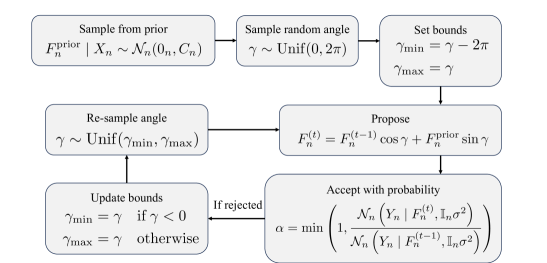
Figure 1: Diagram of one iteration of the ESS algorithm.

It is important to recognize where the work is being done, computationally speaking. Everything except sampling from the prior (top-left) is at worst $\mathcal{O}(n)$ flops, whereas generating $F_{n}^{\mathrm{prior}}$ is $\mathcal{O}(n^{3})$ via Cholesky (Gelman et al.,, 1995, Appendix B). MCMC mixing, that is the diversity of $F_{n}^{(t)}$ relative to $F_{n}^{(t-1)}$, is generally excellent and often it only takes a few iterations to “accept” in the likelihood ratio (bottom-right), after which we update $t\leftarrow t+1$ and move on to the next sample.

For prediction, rather than $F_{n}^{\mathrm{prior}}\mid X_{n}\sim\mathcal{N}_{n}(0_{n},C_{n})$ in the first step, instead draw

$$\left(\begin{array}[]{c}F_{n}^{\mathrm{prior}}\\ \mathcal{F}_{n^{\prime}}^{\mathrm{prior}}\end{array}\right)\sim\mathcal{N}_{n+n^{\prime}}\left(\left[\begin{array}[]{c}0_{n}\\ 0_{n^{\prime}}\end{array}\right],\left[\begin{array}[]{cc}C_{n}&C_{nn^{\prime}}\\ C_{n^{\prime}n}&C_{n^{\prime}}\end{array}\right]\right),$$ (4)

where $C_{n^{\prime}}$ is defined similarly to $C_{n}$ except with inputs $\mathcal{X}_{n^{\prime}}$ and $C_{nn^{\prime}}^{ij}$ involves a kernel calculation on the $i^{\mathrm{th}}$ row of $X_{n}$ and the $j^{\mathrm{th}}$ row of $\mathcal{X}_{n^{\prime}}$. Then, only use $F_{n}^{\mathrm{prior}}$ in subsequent calculations for ESS following the diagram in Figure 1. When eventually an acceptable combination of previous/prior sample is “accepted”, return $\mathcal{F}_{n^{\prime}}^{(t)}=\mathcal{F}_{n^{\prime}}^{(t-1)}\cos\gamma+\mathcal{F}_{n^{\prime}}^{\mathrm{prior}}\sin\gamma$ as the next sample of the unknown function at $\mathcal{X}_{n^{\prime}}$.

An illustration

To illustrate, consider a simple logistic response in one input dimension observed with a small amount of noise at $n=20$ equally-spaced inputs $X_{n}$. The left panel in Figure 2 shows the outcome of five samples via ESS starting with an initial $F_{n}^{(0)}\approx 5$, i.e., constant, indicating no relationship between $x$ and $y$. Ignore the right panel for now. That, and other details for this visual are deferred to Section 3.2 so as not to detract from the focus on $F_{n}$.

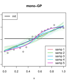
Figure 2: ESS in 1d. Thick solid lines represent “accepted” ESS samples $F_{n}^{(t)}\mid F_{n}^{(t-1)}$, beginning with $F_{n}^{(0)}=5$. Thinner, dashed lines of the same color represent rejected proposals.

Each thick colored line represents a subsequent $F_{n}^{(t)}$ for some $t$ Thinner, dashed lines of identical color indicate rejected samples within ESS before the thick one was accepted. Observe that it doesn’t take many iterations before one is accepted, and that the chain converges very quickly to something reasonable from a disadvantageous starting position.

Actually, the lines in Figure 2 are not samples $F_{n}^{(t)}$, indexed by just $n=20$ inputs $X_{n}$, but predictive ones $\mathcal{F}_{n}^{(t)}$ on a denser grid $\mathcal{X}_{n^{\prime}}$, as described around Eq. (4). The reason for this is two-fold. One is that with just $n=20$ coordinates, the plotted $F_{n}^{(t)}$ wouldn’t look smooth to the eye. You’d see nineteen small, connected line segments. By using a slightly larger grid $\mathcal{X}_{n^{\prime}}$ with $n^{\prime}=50$, we get line segments (which are technically still there, because that’s how R draws curves from points) that look like samples of a smooth function. The second reason is the converse of the first: a collection of fifty responses on a grid of inputs is enough to convey all relevant information about a function of one input, at least from the perspective of visual perception. This leads us to our first novel idea.

2.3 Reference process for one input

Consider, as in the illustration above, a single input ($p=1$) coded to the unit interval: $X_{n}\in[0,1]^{n}$. Now, create an evenly-spaced grid $X_{g}$ in $[0,1]$, akin to knots or inducing points (Snelson and Ghahramani,, 2006; Banerjee et al.,, 2008) with corresponding $F_{g}$. There is really no difference between the latent process at $X_{g}$ and the one at $\mathcal{X}_{n^{\prime}}$ from the illustration above except that $F_{g}$ is on a pre-determined grid, whereas predictive locations of interest could be anywhere and of any size. In fact, we prefer a grid of size $n_{g}=50$, though ultimately this is a tuning parameter trading off computational effort and resolution. [See Appendix A.2.]

Now, an inducing points approach uses GP conditioning to relate $(X_{g},F_{g})$ to training $(X_{n},Y_{n})$ or testing $(\mathcal{X}_{n^{\prime}},\mathcal{Y}_{n^{\prime}})$. This is coherent from a modeling perspective, but comes at a cubic expense in all sizes: $\mathcal{O}(n^{3}+{n^{\prime}}^{3}+n_{g}^{3})$. Plotting in R could work that way too, but it’s clearly overkill. For most situations, linear interpolation from $(X_{g},F_{g})$ to $X_{n}$ or $\mathcal{X}_{n^{\prime}}$ works great: you can’t tell it’s not a curve with modest $n_{g}$ and the computational cost is greatly reduced: $\mathcal{O}(n_{g}^{3}+n+n^{\prime})$. So this is what we propose to do, but inside MCMC posterior sampling via ESS. Everything is performed on the reference process $(X_{g},F_{g})$, but whenever we need to evaluate a likelihood for $Y_{n}$ or a prediction for $\mathcal{X}_{n^{\prime}}$ we linearly interpolate to $F_{n}$ or $\mathcal{F}_{n^{\prime}}$. Modifications to Figure 1 are as follows: keep track of $F_{g}^{(t-1)}$, propose $F_{g}^{\mathrm{prior}}\mid X_{g}$ (top-left), form $F_{g}^{(t)}=F_{g}^{(t-1)}\cos\gamma+F_{g}^{\mathrm{prior}}\sin\gamma$, but to calculate the acceptance probability (bottom-right) first interpolate to $F_{n}^{(t)}$ and $F_{n}^{(t-1)}$ before evaluating likelihoods.

Actually, you can think about the linear interpolation as being inside the likelihood itself. In this way, it is not an approximation but a totally different model. The part of it that is a GP, i.e., the MVN prior on latent functions, is unchanged: for any inputs $X$ whether that is $X_{g}$, $X_{n}$ or $\mathcal{X}_{n^{\prime}}$, the prior is MVN: $F\sim\mathcal{N}(0,C(X))$, abusing notation somewhat. But when evaluating the likelihood (1) we first “snap” from the reference process to the actual one: $F_{n}=\mathrm{LI}(X_{n},X_{g},F_{g})$, where LI stands generically for linear interpolation, say via approx in R, but any fast interpolator will do. We provide the details of our own in Appendix A.3. This is completed with a prior over the reference latent process $F_{g}\mid X_{g}\sim\mathcal{N}_{n_{g}}(0_{n_{g}},C_{g})$, where $C_{g}$ depends on $X_{g}$ and $\theta$. We shall write out a full hierarchical model, extending Eq. (1), once we add the monotonic ingredient in Section 3. Although the $F_{g}\mid X_{g}$ can have a coarsening effect with small $n_{g}$ [as we explore in Appendix A.1], the model for $Y_{n}$ still uses all data to learn the latent function and hyperparameters, again delayed until Section 3.

We limit our application of this idea to a single input. It may be possible to extend to $p\geq 2$, but we doubt its practicality. Gridding out $[0,1]^{p}$ with the same density as in 1d (e.g., $n_{g}=50)$ would require $n_{g}=50^{p}$ via Cartesian product. Even an un-gridded space-filling set of knots $X_{g}$ would still require large $n_{g}$ to fill the input volume, obliterating any potential computational savings while severely coarsening the reference process. Note that inducing points also present issues in modest $p$ without large $n_{g}$ (e.g., Wu et al.,, 2022). Nevertheless, we find a 1d reference process useful for a class of monotonic additive models [Section 4] and as priors on injective input warpings for DGPs [Section 5]. In those settings it is not just a computational convenience, but a crux of the whole enterprise.

3 Monotonic Gaussian processes

Here we extend the reference process of Section 2.3 to monotonic functions.

3.1 Non-decreasing transformation

Consider again $p=1$ and $X_{n}\in[0,1]^{n}$ but now additionally suppose $X_{n}$ is ordered: $x_{i}\leq x_{i+1}$. Now, we change notation to refer to the Gaussian latent process as $Z$ rather than $F$. That is, let $Z_{n}\sim\mathcal{N}_{n}(0_{n},C_{n})$. A transformation of $Z$ is designed so that $F$ is monotonic in $X$. Many transformations could work well; see commentary in Appendix A.2. Our preferred transformation involves three steps: (1) exponentiate for positivity; (2) cumulatively sum so non-decreasing; (3) normalize to $[0,1]$. In formulas, if $Z^{(0)}\sim\mathcal{N}(0,C)$, then

$$Z^{(1)} =\exp{Z^{(0)}}, z^{(2)}_{i} =\sum_{j=1}^{i}z^{(1)}_{j}, f_{i}\equiv z^{(3)}_{i} =\frac{z^{(2)}_{i}-\min(Z^{(2)})}{\max(Z^{(2)})-\min(Z^{(2)})},$$ (5)

for $i=1,\dots,n$.

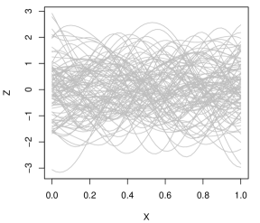
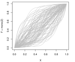
Figure 3: Converting 100 samples from GP prior (left) into monotonic realizations (right).

Figure 3 provides a visual. On the left are ordinary $Z$ from a GP using a lengthscale of $\theta=0.01$, and on the right their monotonically transformed (5) counterparts $F$. The cumulative sum (after ensuring positivity) provides the key non-decreasing ingredient. Post-processing to unity is not essential, but helps inferential details described later.

Yet the cumulative sum is potentially problematic in the context of prediction, which is our main objective. Suppose we have training data at $X_{n}$ and testing locations $\mathcal{X}_{n^{\prime}}$, also ordered. We could apply Eq. (5) to $Z=(Z_{n},\mathcal{Z}_{n^{\prime}})$ drawn as in Eq. (4), but with $Z$s instead of $F$s. Yet we would get different $F_{n}$-values from Eq. (5) depending on whether we transformed $\mathcal{Z}_{n^{\prime}}$ along with the $Z_{n}$ values, and also on which $\mathcal{X}_{n^{\prime}}$ are used.

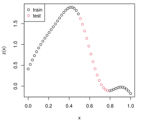
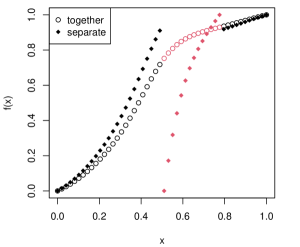
Figure 4: Joint or separated mapping of training and testing $Z$s (left) into $F$s (right).

For example, the left panel of Figure 4 shows a single realization of combined training and testing $Z$-values. Notice that the monotonic $F$-values you get on the right depend on whether you apply Eq. (5) jointly (together for train and test at once) or separately. Also observe that when $\mathcal{X}_{n^{\prime}}$ is heavily concentrated in one part of the input space relative to $X_{n}$ you get a discontinuity in $F_{n}$. We want smooth latent functions, and more broadly we don’t want a model for latent $F_{n}$ that is affected by where you’re trying to predict $\mathcal{X}_{n^{\prime}}$. $F_{n}$ should depend only on $X_{n}$.

The reference process that we introduced in Section 2.3 can fix both things, whereby everything is anchored to one collection $(X_{g},Z_{g})$ via linear interpolation and transformation. Eq. (1) is unchanged; we still have $F_{n}=\mathrm{LI}(X_{n},X_{g},F_{g})$. For prediction we may similarly calculate $\mathcal{F}_{n^{\prime}}=\mathrm{LI}(\mathcal{X}_{n^{\prime}},X_{g},F_{g})$, and in so doing we prevent a choice of predictive locations from affecting training quantities through the cumulative sum. As a bonus, the reference process enjoys all of the computational advantages boasted for ordinary GPs earlier. Note only the reference $X_{g}$ must be ordered in this setup, not $X_{n}$ or $\mathcal{X}_{n^{\prime}}$.

3.2 Full model and posterior inference

Our full mono-GP hierarchical model is provided below.

Likelihood: $$Y_{n}\mid X_{n},F_{n} \sim\mathcal{N}_{n}(\mu+\nu(F_{n}-\textstyle\frac{1}{2}),\mathbb{I}_{n}\sigma^{2}) \mbox{notice the }-\textstyle\frac{1}{2}$$ (6)

$$F_{n} =\mathrm{LI}(X_{n},X_{g},F_{g})$$ say via approx in R

$$F_{g} =\mbox{\tt mono}(X_{g},Z_{g})$$ following Eq. (5)

and Priors: $$Z_{g}\mid X_{g} \sim\mathcal{N}_{n_{g}}(0_{n_{g}},C_{g}) C_{g}\mbox{ depends on $X_{g}$ and $\theta$}$$

$$p(\mu,\sigma^{2}) \propto 1/\sigma^{2}$$ improper Jeffereys prior

$$\nu \sim\mathrm{Gamma}(\alpha_{\nu},\beta_{\nu}) \alpha_{\nu}=\beta_{\nu}=10^{-3}$$ diffuse, e.g.,

$$\theta \sim\mathrm{Gamma}(\alpha_{\theta},\beta_{\theta}) (\alpha_{\theta},\beta_{\theta})=(3/2,5)$$ e.g.,

Some quick commentary is in order. Notice how we center $F_{n}$ around zero by subtracting $1/2$. This is because we normalized to $[0,1]$ as part of Eq. (5), and we wish to interpret $\mu$ as a “centering” location parameter. But it is not essential; we can skip it or instead normalize directly to $[-0.5,0.5]$. Our choices here are motivated by a compromise between modeling goals in Section 3–4 and our deep GP application in Section 5.

Linear interpolation (LI) and the monotonic transformation (mono) could be composed into a single step, as $\mathrm{LI}(X_{n},X_{g},\mathrm{mono}(X_{g},Z_{g}))\equiv\mbox{\tt monoref}(X_{n},X_{g},Z_{g})$, and this is how it is in our implementation. We never need to do one without the other, but we thought it helpful to have them separate in Eq. (6). Both are completely deterministic, working together to define a GP prior on the latent random function $f(x)$. In our posterior sampling scheme described momentarily, we only save $Z_{g}^{(t)}$-values as everything else we need, like $F_{n}^{(t)}$ and $\mathcal{F}_{n^{\prime}}^{(t)}$, can be derived from these through monoref.

A Jeffereys prior for location-scale models (see, e.g., Hoff,, 2009) yields a proper posterior for $n>1$ and may be upgraded to Normal-Inv-Gamma if desired. Both are conditionally conjugate for the Gaussian likelihood, allowing $\mu$ and $\sigma^{2}$ to be integrated out. Let

$$\hat{\mu} =\frac{1}{n}\sum_{i=1}^{n}y_{i}-\nu(f_{i}-\textstyle\frac{1}{2}) s^{2} =\frac{1}{n-1}\sum_{i=1}^{n}(y_{i}-\hat{\mu}-\nu(f_{i}-\textstyle\frac{1}{2}))^{2}$$ and (7)

denote summary statistics for residual location and scale. A marginal likelihood follows

$$p(Y_{n}\mid F_{n},\nu)=\int\!\!\int\mathcal{N}_{n}(Y_{n}\mid\mu+\nu(F_{n}-\textstyle\frac{1}{2}),\mathbb{I}_{n}\sigma^{2})\frac{1}{\sigma^{2}}\,d\mu d\sigma^{2}\propto\left(\frac{(n-1)s^{2}}{2}\right)^{-\frac{n-1}{2}}.$$ (8)

This is a relatively standard result, so we don’t provide derivation details.

What’s non-standard is its use within ESS sampling for $F_{n}$ and Metropolis for $\nu$. Conditional on a $\nu^{(t-1)}$ and $Z_{g}^{(t-1)}$, we may use $Z_{g}^{\mathrm{prior}}$ and ultimately Eq. (3) in the likelihood ratio (bottom-right bubble in Figure 1) via $Z_{g}^{(t)}\rightarrow F_{g}^{(t)}\rightarrow F_{n}^{(t)}$ and $Z_{g}^{(t-1)}\rightarrow F_{g}^{(t-1)}\rightarrow F_{n}^{(t-1)}$ to eventually accept $Z_{g}^{(t)}$. Finally, conditional on $Z_{g}^{(t)}$ via $F_{n}^{(t)}$, a random-walk proposal such as $\nu^{\prime}\sim\mathrm{Unif}[\nu^{(t-1)}/2,2\nu^{(t-1)}]$ may be accepted as $\nu^{(t)}=\nu^{\prime}$ with probability

$$\alpha(\nu^{(t)},\nu^{\prime})=\frac{p(Y_{n}\mid F_{n}^{(t)},\nu^{\prime})}{p(Y_{n}\mid F_{n}^{(t)},\nu^{(t-1)})}\times\frac{\mathrm{Gamma}(\nu^{\prime};\alpha_{\nu},\beta_{\nu})}{\mathrm{Gamma}(\nu^{(t-1)};\alpha_{\nu},\beta_{\nu})}\times\frac{\nu^{(t-1)}}{\nu^{\prime}},$$ (9)

or otherwise $\nu^{(t)}=\nu^{(t-1)}$. Posterior sampling for $\theta$ is similar. Conditional on all other quantities, a proposal $\theta^{\prime}\sim\mathrm{Unif}[\theta^{(t-1)}/2,2\theta^{(t-1)}]$ may be accepted as $\theta^{(t)}=\theta^{\prime}$ with probability

$$\alpha(\theta^{(t)},\theta^{\prime})=\frac{p(Z_{g}^{(t)}\mid\theta^{\prime})}{p(Z_{g}^{(t)}\mid\theta^{(t-1)})}\times\frac{\mathrm{Gamma}(\theta^{\prime};\alpha_{\theta},\beta_{\theta})}{\mathrm{Gamma}(\theta^{(t-1)};\alpha_{\theta},\beta_{\theta})}\times\frac{\theta^{(t-1)}}{\theta^{\prime}},$$ (10)

where $p(Z_{g}\mid\theta)$ is the pdf of $\mathcal{N}_{n_{g}}(Z_{g};0_{n_{g}},C_{g})$ where $C_{g}$ is built from $\theta$. The entire Metropolis-within-Gibbs algorithm is encapsulated in Algorithm 1 for convenience.

Initialize $Z_{g}^{(0)}$, $\theta^{(0)}$, $\nu^{(0)}$.

for $t=1,\dots,T$ do

       Sample $Z_{g}^{(t)}\mid Z_{g}^{(t-1)},\nu^{(t-1)},\theta^{(t-1)}$ via ESS (Figure 1), marg. lik. (3) and $(\hat{\mu},s^{2})$ (7).

       Sample $\nu^{(t)}\mid Z_{g}^{(t)}$ via MH (9), marg. lik. (3) and $(\hat{\mu},s^{2})$ (7).

       Sample $\theta^{(t)}\mid Z_{g}^{(t)},\theta^{(t-1)}$ via MH (10)with MVN pdfs using $C_{g}$ for each $\theta$.

Algorithm 1 MCMC (Metropolis-within-Gibbs) for mono-GP.

Prediction at $\mathcal{X}_{n^{\prime}}$ is a simple matter of running back through the MCMC samples, possibly after discarding for burn-in and thinning, to form

$$\mathcal{F}_{n^{\prime}}^{(t)} =\mbox{\tt monoref}(\mathcal{X}_{n^{\prime}},X_{g},Z_{g}^{(t)})$$

$$\mbox{ yielding }\quad\mathcal{Y}_{n+1}^{(t)} \sim\mathrm{St}_{n^{\prime}}(\hat{\mu}^{(t)}+\nu^{(t)}(\mathcal{F}_{n^{\prime}}^{(t)}-\textstyle\frac{1}{2}),\mathbb{I}_{n^{\prime}}(1+\textstyle\frac{1}{n})s^{2(t)},n-1),$$ (11)

where St is a location-scale Student-$t$ distribution with degrees of freedom $n-1$. Moments $\hat{\mu}^{(t)}$ and $s^{2(t)}$ follow Eq. (7) with $\hat{\nu}^{(t)}$ and $F_{n}^{(t)}$ values plugged in. Although written implying a multivariate density, a diagonal covariance means it can be handled element-wise in scalar form. For most applications, full posterior predictive samples (11) are overkill. When benchmarking via RMSE or scoring rules, we use moment-based aggregates:

$$\hat{\mu}(\mathcal{X}_{n^{\prime}}) =\frac{1}{T}\sum_{t=1}^{n}\hat{\mu}^{(t)}+\nu^{(t)}(\mathcal{F}_{n^{\prime}}^{(t)}-\textstyle\frac{1}{2})$$ (12)

$$\Sigma(\mathcal{X}_{n^{\prime}}) =\mathbb{C}\mathrm{ov}\left[\hat{\mu}^{(t)}+\nu^{(t)}(\mathcal{F}_{n^{\prime}}^{(t)}-\textstyle\frac{1}{2})\right]_{t=1}^{T}+\mathbb{I}_{n^{\prime}}\times\frac{1}{T}\sum_{t=1}^{T}s^{2(t)}\times\frac{(n-1)}{(n-3)}.$$

Notice how these reveal spatial dependence in predictions explicitly through the covariances on the mean via the law of total variance. The change in denominator from $n-1$ to $n-3$ arises from the expression for Student-$t$ variance. All predictive calculations are linear in $n$, $n^{\prime}$ and $T$ except $\mathbb{C}\mathrm{ov}$ in Eq. (12) provided posterior samples following Alg. 1. If the $\mathcal{O}({n^{\prime}}^{2})$ cost of $\mathbb{C}\mathrm{ov}$ is prohibitive, a linear-cost pointwise variance may be calculated instead.

An illustration

Recall the visual provided in Figure 2. The true data-generating mechanism is

$$Y(x)=\frac{10\exp(10x-5)}{1+\exp(10x-5)}+\varepsilon_{i}\quad\mbox{ where }\quad\varepsilon_{i}\stackrel{{\scriptstyle\mathrm{iid}}}{{\sim}}\mathcal{N}(0,1)\quad\mbox{ and }x\in[0,1].$$

In other words, it is within our assumed model class with $(\mu,\nu,\sigma^{2})=(0,10,1)$, and $f(x)=\mathrm{logit}^{-1}(10x-5)$. For posterior sampling, and actually for all MCMC in Sections 3–4, we take $T=5000$ total samples, discard the first $B=1000$ as burn-in and thin to take every $10^{\mathrm{th}}$, implicitly re-defining $T=400$. Throughout we use $X_{g}\in[0,1]$ with $n_{g}=50$. The right panel of Figure 2 shows monoref versions of ESS samples along $X_{g}$. Note there are fewer dashed lines in the right panel, indicative of faster ESS acceptance.

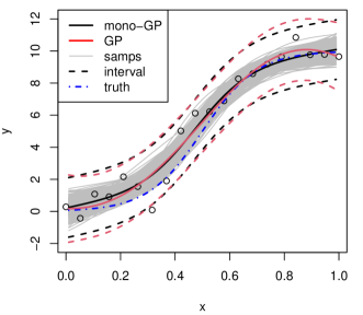
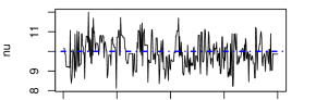
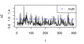
Figure 5: Predictive surfaces (left), with mono-GP posterior samples $F_{n}^{(t)}$ as gray lines, and MCMC trace-plots (right) for 1d logistic example.

The left panel of Figure 5 completes the picture by showing samples from the (shifted $\mu$ and scaled $\nu$) latent function $\mathcal{F}_{n^{\prime}}$ in gray, along with predictive means and quantiles derived from posterior averages of Eq. (11). Predictive $\mathcal{X}_{n^{\prime}}$ vary by example, and for this $\mathrm{logit}^{-1}$ one we used a regular $n^{\prime}=100$-sized grid. For comparison, a regular GP – with analytically marginalized latents via laGP (Gramacy,, 2016) – is shown in red. While the GP is highly accurate, it is not monotonic. The trace plots in the right panel(s) of Figure 5 show that MCMC mixing is good for $\nu^{(t)}$ and for (the derived quantity) $s^{2(t)}$, and they also hover around their true values. Trace plots for $\mu^{(t)}$ are similar, but not shown. Traces $\theta^{(t)}$ also indicate good mixing (not shown), but there is no true value to compare to directly. Latent $\mathcal{F}_{n^{\prime}}^{(t)}$ (gray/left panel), which come indirectly from those $\theta^{(t)}$, capture the truth well.

4 Additive framework for multiple inputs

Extending monotonicity to more inputs is nuanced since there is no natural ordering on $\mathbb{R}^{p}$ for $p\geq 2$. Here we consider the simplest possible extension of coordinate-wise monotonicity.

4.1 Bayesian modeling and inference

We capture this coordinate-wise notion in a statistical model as follows. Let $X_{n}$ be $n\times p$ with rows $x_{i}^{\top}=(x_{i1,},\dots,x_{ip})^{\top}$, for $i=1,\dots n$. Then presume $y_{i}=\mu+\sum_{j=1}^{n}\nu_{j}f_{j}(x_{ij})+\varepsilon_{i}$, with $\varepsilon_{i}\stackrel{{\scriptstyle\mathrm{iid}}}{{\sim}}\mathcal{N}(0,\sigma^{2})$ where $f_{j}(x_{ij})\leq f_{j}(x_{kj})$ for $x_{ij}\leq x_{kj}$, and $v_{j}>0$ for all $j=1,\dots,p$. In other words, all $f_{j}$ are 1d monotonic functions, and their linear combination involves only positive coefficients $\nu_{j}$. Observe that the $p=1$ case of Section 3 is nested within this setup.

This setup also resembles López-Lopera et al., (2022), but our fully hierarchical model and inferential apparatus are quite distinct. We prescribe $p$ independent but otherwise identical copies of everything in Eq. (1) except the likelihood (which is unchanged). That is, let $F_{n}$ be $n\times p$ like $X_{n}$ where the $j^{\mathrm{th}}$ column of $F_{n}$ corresponds to the $j^{\mathrm{th}}$ a priori independent process on the $j^{\mathrm{th}}$ column $X_{n}^{\cdot j}$ of $X_{n}$. Then let $\nu=(\nu_{1},\dots,\nu_{p})^{\top}$ denote a $1\times p$ row-vector of a priori independent scales. Using these quantities, interpret the likelihood in Eq (1) as a vector-matrix product in $\nu(F_{n}-\textstyle\frac{1}{2})$, where $\frac{1}{2}$ subtracts off every element of $F_{n}$.

Duplicating (actually $p$-licating) the other lines of Eq. (1) requires some care. We use an identical 1d reference grid $X_{g}$ for each coordinate, $j=1,\dots,p$, but with distinct lengthscales $\theta=(\theta_{1},\dots,\theta_{p}$), in keeping with an automatic relevance determination (ARD; Rasmussen and Williams,, 2006)-like setup. So the full set of unknowns is $\mu,\sigma^{2},\nu,\theta$ as before, but $\nu$ is now vectorized. This makes inference a straightforward extension of Section 3.2. MCMC basically follows Alg. 1 in $p$-licate via the following summary statistics extending Eq. (7).

$$\hat{\mu} =\frac{1}{n}\sum_{i=1}^{n}y_{i}-\sum_{j=1}^{p}\nu_{j}(f_{ij}-\textstyle\frac{1}{2}) s^{2} =\frac{1}{n-p}\sum_{i=1}^{n}(y_{i}-\hat{\mu}-\sum_{j=1}^{p}\nu_{j}(f_{ij}-\textstyle\frac{1}{2}))^{2}$$ and (13)

Above, $\nu(F_{n}-\frac{1}{2})$ is written out explicitly in sum-form for clarity. Similarly, predictions via Eq. (11–12) may be applied identically with $n-p$ for $n-1$, including $n-p-2$ for $n-3$. Again, this setup nests $p=1$ as a special case.

An illustration

Consider a $p=2$ upgrade to our running logistic example from earlier sections. We shall benchmark in higher dimension momentarily in Section 4.2. Take $f_{1}(x)=\mathrm{logit}^{-1}(10x-7)$ and $f_{2}(x)=\mathrm{logit}^{-1}(10x-3)$ with $\nu=(10,5)$, differentially shifting and scaling the 1d version. Complete the setup with $(\mu,\sigma^{2})=(0,0.1)$. Training $X_{n}$ are taken from a Latin hypercube sample (LHS; McKay et al.,, 2000) of size $n=100$ in 2d.

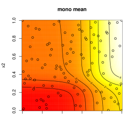
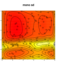
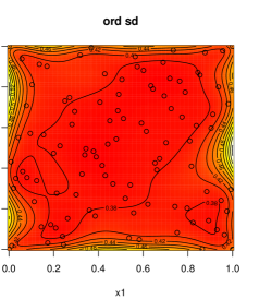
Figure 6: 2d logistic fits from a monotonic additive GP (mono-GP, top row) to an ordinary GP (via laGP, bottom row) on mean (left) and SD (right). Red is low and white is high, with novel color palettes in each panel.

We then make predictions on a $100\times 100$ grid $\mathcal{X}_{n^{\prime}=10\mathrm{K}}$ to support visuals like those in Figure 6 which offer a comparison between our monotonic additive GP (still mono-GP, top row) and an ordinary GP (with ARD, bottom row). Focus first on the left column, showing predictive means. Despite superficial similarities, notice how contour lines for the ordinary GP wiggle: telltale departure from monotonicity. Now look at the the standard deviations on the right. The ordinary GP exhibits typical behavior with increasing uncertainty in distance to nearby training data (open circles). Mono-GP exhibits a more nuanced spatial UQ, seeming to be aligned with regions where the response is changing most quickly.

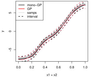
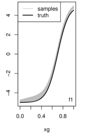
Figure 7: Diagonal slice of 2d logistic predictive surface (left) and mono-GP latent functions in each input compared to the truth (middle and right).

Figure 7 shows three 1d views, first comparing mono-GP to the ordinary GP along the $x_{1}=x_{2}$ slice, and then coordinate-wise for columns of $F_{n}$ over $X_{g}$. Observe on the left a view similar to the left panel of Figure 5. As in that case, the surfaces are similar but the one from the ordinary GP is not monotonic, particularly at the two corners of the input space. The middle and right panels show samples of columns of $F_{n}$ relative to the truth: our latent functions are generally capturing the true data-generating mechanism.

4.2 Implementation and benchmarking

Here we upgrade our earlier, largely visual illustrations into a series of benchmarking exercises. Metrics include RMSE to the truth, and continuous ranked probability score (CRPS; Gneiting and Raftery,, 2007) to noisy testing realizations. Our implementation of mono-GP requires about 200 lines of pure R code, using add-on libraries only for MVN deviates via mvtnorm on CRAN (Genz and Bretz,, 2009) and distance calculation via laGP. Our monotonic competitor, lineq-GP, is facilitated by R code provided by López-Lopera et al., (2022), via lineqGPR (Lopez-Lopera,, 2022), without modification. As earlier, we use laGP, which is predominantly in C, for an ordinary GP. The 1d logistic example from earlier is relegated to Appendix B.1 because it is uninteresting. Appendix B.3 provides timing comparisons varying $n$ and $n^{\prime}$, however pitting C against R is like apples to oranges.

2d logistic

We begin with the 2d logistic variation introduced above in Section 4. The experimental setup here is identical to that one, where each new Monte Carlo (MC) instance uses a novel LHS of size $n=100$ paired with novel error deviates on the response. We use 30 MC repetitions throughout. This 2d example uses the fixed $n^{\prime}=10\mathrm{K}$ testing grid described above, whereas our other higher dimensional examples use LHSs.

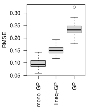
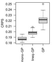
Figure 8: Metrics on the 2d logit MC experiment. Smaller is better for all.

Figure 8 collects the results. Observe that the monotonic methods outperform an ordinary GP (lower RMSE/CRPS), and that our mono-GP edges out the lineq-GP from Lopez-Lopera,. It is worth nothing that lineqGPR was not created for bakeoffs of this kind. The method targets a wider class of constrained problems and emphasizes active learning applications.

5d Lopez–Lopera

Our remaining examples come from López-Lopera et al., (2022) and use $p=5$ and $p=10$, respectively. Both can be seen as inherently logistic in nature, though with slightly different emphasis on coordinates. The first one follows

$$y(x)=\mathrm{atan}(5x_{1})+\mathrm{atan}(2x_{2})+x_{3}+2x_{4}^{2}+\frac{2}{1+\exp(-10(x_{5}-\textstyle\frac{1}{2}))}+\varepsilon,\quad\varepsilon\stackrel{{\scriptstyle\mathrm{iid}}}{{\sim}}\mathcal{N}(0,0.1^{2}).$$

Like the 2d logistic above, this can be re-expressed in our additive model class. Figure 9 summarizes the outcome of a MC experiment based on novel $n=100$ training and $n^{\prime}=1000$ testing LHSs.

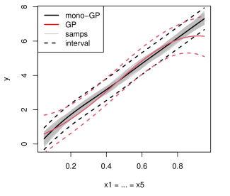
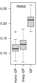
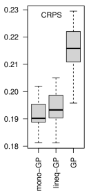
Figure 9: Diagonal visual (left) and metrics on the 5d Lopez–Lopera MC experiment.

Observe that mono-GP and lineq-GP are similar on RMSE and CRPS, yet in only one of the thirty reps was mono-GP inferior to lineq-GP on either metric. Consequently, a one-sided paired Wilcoxon test rejects similarity with $p=1.3\times 10^{-8}$. The left panel shows predictive surfaces along the diagonal, confirming that the ordinary GP is unable to learn that the response surface is non-decreasing.

Figure 10: Comparison of mono-GP latent functions for 5d Lopez–Lopera example to the truth.

Figure 10 shows the latent functions learned for each input coordinate compared to the truth. It is nice to have this interpretive aspect to our mono-GP implementation. We could couple that with the amplitudes provided by $\nu^{(t)}$ [see Appendix B.4], but we prefer here to show each on the same $y$-axis. With ordinary GPs, it can be difficult to tease out the relative contributions of each input, say via an ex post sensitivity analysis (e.g., Saltelli et al.,, 2000; Marrel et al.,, 2009; Oakley and O’Hagan,, 2004; Gramacy,, 2020, Chapter 9.1). With mono-GP a coordinate-wise breakdown is implicit in its construction.

10d Lopez–Lopera arctan

Our next López-Lopera et al., example is originally from Bachoc et al., (2022).

$$y(x)=\sum_{j=1}^{p}\mathrm{atan}\left(5\left[1-\frac{1}{p+1}\right]x_{j}\right)+\varepsilon,\quad\varepsilon\stackrel{{\scriptstyle\mathrm{iid}}}{{\sim}}\mathcal{N}(0,0.1^{2})$$

Here we consider the $p=10$ case. Other things from previous experiments are unchanged, and Figure 11 summarizes the results of our MC benchmarking exercise.

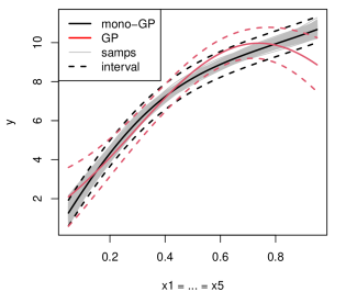
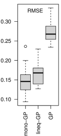
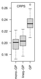
Figure 11: Diagonal visual (left) and metrics on the 5d Lopez–Lopera MC experiment.

Again, it is obvious that an ordinary GP is inferior (boxplots on right) because it is unable to leverage that the response surface is monotonic (left). Mono-GP and lineq-GP are similar, but again mono-GP is only inferior twice out of thirty times by either metric leading to $p=9.3\times 10^{-9}$, rejecting parity. A coordinate-wise sensitivity analysis via columns of $F_{n}$ is provided in Appendix B.4.

5 Monotonic warpings for deep GPs

Deep Gaussian processes (DGPs) originate in spatial statistics (e.g., Sampson and Guttorp,, 1992; Schmidt and O’Hagan,, 2003) for non-stationary modeling (e.g., Paciorek and Schervish,, 2003; Sauer et al.,, 2023a), and have been recently re-popularized in ML (Salimbeni and Deisenroth,, 2017; Bui et al.,, 2016; Cutajar et al.,, 2017; Laradji et al.,, 2019) by analogy to deep neural networks (DNNs). Here we focus on Sauer et al., (2023c) whose fully Bayesian DGP provides the UQ necessary for many surrogate modeling applications of interest to us. Sauer et al.,’s ESS-based inferential framework laid the groundwork for our monotonic setup in Section 3.1. We provide a brief DGP review here, with the minimum detail required to explain our contribution. As a disclaimer, note that we are pivoting back to ordinary (not monotonic) regression, with mono-GP featuring as an important subroutine.

All of the modeling “action” for a conventional GP, generically $Y\sim\mathcal{N}(0,\Sigma(X))$, resides in $\Sigma(X)$. When the kernel depends on displacement only, i.e., $\Sigma^{ij}=\Sigma(x_{i}-x_{j})$, the resulting process is said to be stationary. This means that the positions of inputs in $X$ don’t matter, only the gaps between them. Consequently, when making predictions at new inputs $\mathcal{X}_{n^{\prime}}$, only the displacements between training and testing sets matter, not their raw locations. This, in turn, means that you can’t have different “regimes” in the input space where input–output dynamics exhibit diverse behavior. Stationarity is a strong, simplifying assumption, that can be prohibitive in many modeling contexts. For example, fluid dynamics simulations can exhibit both equilibrium and turbulent behavior depending on their configuration. A stationary GP could not accommodate both. We consider an example later that involves modeling a rocket booster re-entering the atmosphere (Pamadi et al.,, 2004) where low-speed lift dynamics differ from high-speed ones.

A DGP uses two or more stationary GPs in a chain. One (or more) warps the inputs into a regime where a stationary relationship is plausible, which is then fed into another GP for the response, e.g., $W_{n}\sim\mathcal{N}(0,\Sigma(X_{n}))$ feeding into $Y_{n}\sim\mathcal{N}(0,\Sigma(W_{n}))$. When there are multiple inputs, it is common to match latent and input dimension, specifying $X\rightarrow W^{\cdot j}$, for $j=1,\dots,p$ with $W^{\cdot j}\stackrel{{\scriptstyle\mathrm{iid}}}{{\sim}}\mathcal{N}(0,\Sigma(X))$. In other words, the $j^{\mathrm{th}}$ coordinate of $W$ is determined by (all of) $X$. Here we restrict our attention to such “two-layer” DGPs. The difficult thing about DGP inference is integrating out the $n$-dimensional warping variables $W^{\cdot j}$. Twenty years ago Schmidt and O’Hagan, (2003) tried Metropolis-based methods, but to say it was cumbersome is an understatement. Recent ML revivals focus on variational inference methods with inducing points approximations, but these undercut on both fidelity and UQ. For computer simulation experiments, ESS seems ideal. MVN priors ($W^{\cdot j}\mid X$) paired with MVN likelihood ($Y\mid W$) means we can follow Figure 1 in $p$-licate.

5.1 Component swap

Such two-layer DGPs are still supremely flexible. Every coordinate of $X$ informs each $W^{\cdot j}$, and the relationship between them can be pretty much any (stationary) function. Here, we argue that for many computer simulation experiments some additional regularization is advantageous. We propose warping each $X^{\cdot j}$ to $W^{\cdot j}$ via mono-GP rather than a full GP. In other words, apply the $p$ copies of Section 3.1 for a coordinate-wise injective warping. Since only relative distances matter between (even warped) inputs, we fix $(\mu,\nu,\sigma^{2})=(0,1,0)$ and we don’t do $-\frac{1}{2}$ so that $W\in[0,1]$. Since each $W^{\cdot j}$ is equivalently scaled, the outer GP ($Y\mid W$) requires separable lengthscales, an upgrade from Sauer et al.,’s original implementation. We call this the “mw-DGP” where “mw” is for “monowarp”.

An illustration

Consider the “cross-in-tray” function, which can be found in the Virtual Library of Simulation Experiments (VLSE; Surjanovic and Bingham,, 2013). We follow the typical setup

$$f(x)=-0.0001\left(\left|\sin(x_{1})\sin(x_{2})\exp\left\{\left|100-\frac{\sqrt{x_{1}^{2}+x_{2}^{2}}}{\pi}\right|\right\}\right|+1\right)^{0.1}\quad\mbox{ with }\quad x\in[-2,2]^{2},$$

but coded to the unit cube. A non-stationary GP is essential because there are both steep (cross) and flat (tray) regions. We train on an LHS of size $n=40$ and predict on a dense 2d grid of size $n^{\prime}=900$. Throughout our DGP-based experiments we use deepgp-package defaults (i.e., 10K MCMC samples), discarding 1K as burn-in and thinning by 10 for $T=900$ total. Basically we use fit_two_layer with and without a new option: monowarp = TRUE.

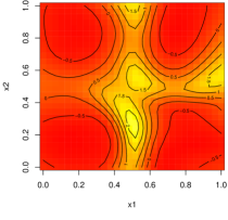
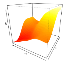
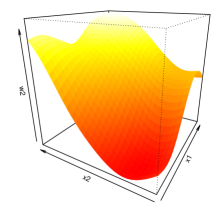
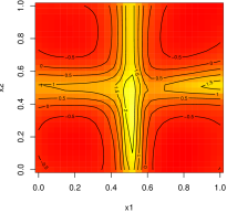
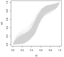
Figure 12: DGP (top row) and mw-DGP (bottom row) on cross-in-tray. Columns provide predictive mean (left) and warpings $W^{\cdot 1}$ and $W^{\cdot 2}$ (middle and right, respectively).

Figure 12 summarizes our fits visually, with an ordinary DGP in the top row of panels and mw-DGP on the bottom. The left column shows predictive means. The true surface makes an axis-aligned cross, so the mw-DGP is doing a better job of capturing that. We shall provide full benchmarking results momentarily. Observe in the top-right panels that the warpings from DGP are not monotonic. Here we are showing just one sample of $W^{(t)}$ since these are in 2d. Observe that both samples have multiple regions where they fold back on one another. On the bottom we show all posterior samples of coordinate-wise monotonic warpings. They indicate that the middle of the input space (the cross) is stretched relative to the edges (tray), which is supported by the views shown on the left.

5.2 Benchmarking

Here we provide out-of-sample metrics for three examples (with a fourth in Appendix B.2), all summarized in Figure 13, beginning with cross-in-tray from Section 5.1 in the left/first column. Since we have already introduced that example, we do not provide a separate heading for it here. We simply remark that the setup is identical to that earlier description, except that we repeated it in a MC fashion thirty times, as with the other examples.

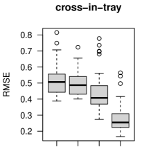
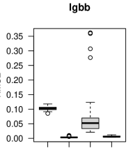
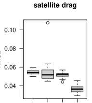
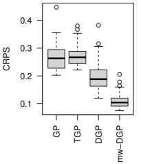
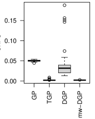
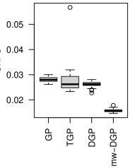
Figure 13: Non-stationary benchmark out-of-sample metrics. Smaller is better for all.

In addition to an ordinary DGP, we include a stationary GP via the same MCMC apparatus as DGP, using fit_one_layer in deepgp, and a treed Gaussian process (TGP) via the tgp package on CRAN (Gramacy,, 2007; Gramacy and Taddy,, 2010) using btgpllm with defaults. The first/left column of Figure 13 shows that mw-DGP convincingly outperforms the other competitors on cross-in-tray. Although mw-DGP utilizes the thriftier $n_{g}$-sized reference process for $W$, an ordinary $n$-sized GP is still used on the outer layer. Despite being $\mathcal{O}(n^{3})$ like the other methods, many fewer such operations mean a faster execution. Appendix B.3 provides detailed timings including Vecchia upgrades (Sauer et al.,, 2023b).

Rocket booster

The second column of Figure 13 is for the Langley Glide-Back Booster (LGBB; Pamadi et al.,, 2004). The LGBB simulator models aeronautically relevant forces as a rocket booster re-enters Earth’s atmosphere as a function of its speed (mach number), angle of attack, and side slip angle. Here we study the lift force as predicted by those $p=3$ input variables. Gramacy and Lee, (2008)’s TGP was originally developed for the LGBB because it exhibits non-stationary dynamics which manifest as coordinate-wise regime changes in speed and angle of attack. Access to novel simulations for LGGB is no longer possible (previously, runs could only be obtained on NASA’s Columbia supercomputer), so here we use a corpus of 780 training runs provided by Gramacy and Lee, (2009) and subsamples of a densely interpolated set of testing $>37$K outputs provided by a TGP fit from that same paper. For more detail see Gramacy, (2020, Chapter 2). Here we use all simulation outputs as training data $(n=780)$ and a random subsample of TGP predictions for testing $(n^{\prime}=1000)$.

Results are provided in the middle/second column of panels in Figure 13. TGP is a gold standard in this context, having chosen the training data via active learning, and produced the testing output used for benchmarking. Nevertheless, mw-DGP performs nearly as well as TGP, and both are much better than the others. Observe that, at least in some cases, mw-DGP is able to provide better UQ (lower CRPSs) than TGP. We believe this happens because TGP makes inefficient use of the data when partitioning, whereas mw-DGP is able to capture the same spirit of axis-aligned nonstationarity without imposing hard breaks.

Satellite drag

Our final example involves simulations of atmospheric drag for the Gravity Recovery and Climate Experiment (GRACE) satellite in low-Earth orbit (Mehta et al.,, 2014) via a corpus of one million LHS-based runs provided by Sun et al., (2019). These data/simulations involve $p=7$ inputs, and here we consider randomly sub-sampled GRACE runs in pure Hydrogen of size $(n,n^{\prime})=(550,1000)$. As the model is not deterministic, fifty training runs are replicated to provide each model a measure of the uncertainty in the simulation. The results are shown in the right/third column of panels of Figure 13. In contrast to our previous examples, there is no reason to suspect that it might be advantageous to limit non-stationary modeling to axis-aligned dynamics, monotonic or otherwise, beyond the regularization that implies. In fact, observe in the figure that TGP, with its axis-aligned splits, performs worst of all in some cases. A DGP is better than both TGP and an ordinary GP, but in the latter perhaps not by an impressive margin. Nevertheless, mw-DGP is by far the best by both metrics.

6 Discussion

We have provided a new prior on monotonic Gaussian processes (GPs) for a single input variable that we illustrate is valuable for two disparate classes of problems: additive monotonic GPs for multiple inputs and as intermediate warpings for deep GPs (DGPs). There are two key ingredients that make this work well and which distinguish it from earlier approaches to mono-GP. One is a reference process that limits computational effort in the face of cubic computational bottlenecks, and which is essential for our cumulative-sum-based monotonic transformation. The other is elliptical slice sampling (ESS), a powerful but often overlooked MCMC mechanism that is ideally suited to high-dimensional multivariate normal sampling. We showed that our mono-GPs and our monowarped DGPs (mw-DGPs) outperform ordinary GP and DGP alternatives. In our Appendix we also show that our methods are faster, except perhaps on the smallest problems.

We speculate that other simple constraints on GPs (and DGP warpings), besides monotonicity, can be handled in a similar way, as long as a transformation can be used in conjunction with ESS. This could be particularly powerful in small-data contexts, e.g., with expensive computer simulations where much is known about the physics. It may additionally be possible to expand mono-GP to multiple inputs by some construct other than additively. For example, it may be worth exploring active subspace-based GPs (Wycoff,, 2023) in order to rotate into an appropriate axis-aligned regime.

Acknowledgments

RBG and SDB are grateful for funding from NSF CMMI 2152679. This work has been approved for public release under LA-UR-24-28080. SDB, DO and LJB were funded by Laboratory Directed Research and Development (LDRD) Project 20220107DR.

Appendix A Additional methodological details

Here we provide some auxiliary analysis and implementation notes supporting method choices described in the main body of our manuscript.

A.1 Choosing reference grid density

Below we provide two views into accuracy as the size $n_{g}$ of the reference grid $X_{g}$ is increased. The first is visual, and the second based on out-of-sample accuracy. Figure 14 shows views of the 1d logistic predictive surface as $n_{g}$ is varied in $\{10,20,50,100\}$. Otherwise we use the same setup as our illustration in Section 3.1 with the exception of doubling the number of MCMC iterations in order to stabilize RMSE calculations.

Figure 14: 1d logistic for varying $n_{g}$.

Observe in the left-most panel, corresponding to $n_{g}=10$, that the linear interpolation in the mean/black line is visibly detectable. It may also be visible in the second panel, corresponding to $n_{g}=20$, depending on screen resolution/magnification or printer quality. When we zoom in on a high-quality laptop screen we can see the line segments in the $n_{g}=20$ plot. But this is not the case for either of the the right pair of panels.

Now consider accuracy out-of-sample, provided in the bottom-right of each panel. This number seems unaffected by $n_{g}$. These results come from just one repetition, so there is MC error which remains unaccounted for, but hold that thought. Computing time, also provided in the bottom-right, is very much affected by $n_{g}$, especially moving from $n_{g}=50$ to $n_{g}=100$, with the latter being quite extreme by contrast. So we settled on $n_{g}=50$ as a default. It is worth remarking that $n_{g}$ also has an impact on the amount of storage required to retain samples from latent $F_{g}$ for later use.

Next we pivot to a more exhaustive study on a more challenging, high-dimensional problem: Lopez–Lopera 5d from Section 4. We vary $n_{g}$ as above, and track RMSE and computing time.

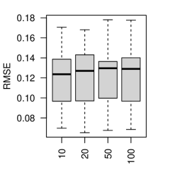
Figure 15: Varying $n_{g}$ on Lopez–Lopera 5d.

Figure 15 collects the resulting metrics. It appears that $n_{g}$ has no detectable effect on accuracy, but a profound one on execution time past $n_{g}=50$ or so. It could be that by choosing an even smaller $n_{g}$ for our experiments throughout the paper we would have had the same accuracy and UQ, but a much faster execution time (our comparison in Appendix B.3 might have come out more favorably for small $n$).

A.2 Variations on the monotonic transformation

We experimented with several variations on the mono-GP prior, and here we report comparatively on two which percolated to the top. The first is the one summarized in Section 3.1 and described in Eq. (5). The second is very similar, but instead of pre-exponentiating, we subtract off the minimum, i.e, $Z^{(1)}=Z^{(0)}-\min Z^{(0)}$. This has the same overall effect of forcing positivity, but it does so linearly.

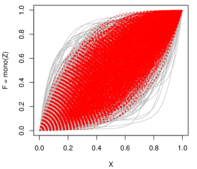
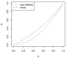
Figure 16: Converting 1000 samples from GP prior in two ways (left) and doing the same thing to the identity map (right).

Figure 16 provides a comparison between these two priors as regards 1d monotonic functions. The left panel of the figure shows 1000 samples from the prior, in gray for Eq. (5) and in red dashed for the new “linear” version. Observe how the spread of gray lines is wider. We liked this because it implied a more diffuse prior over random monotonic functions.

On the right we show how an identity functional relationship maps under the two transformations. The identity is important for our DGP warping application [Section 5], where in that context it means that the $X=W$, i.e., a null warping, implying an ordinary stationary GP – a sensible base case (Sauer et al.,, 2023c). Observe in the right panel that both priors add some curvature to the identity, but that it is more pronounced for the red “linear” option, which may at first be counter-intuitive. The curvature is coming from the cumulative sum in Eq. (5), and by pre-exponentiating we are undoing some of that curvature.

A.3 Bespoke linear interpolation

R’s built-in approx function provides linear interpolation, but it has two downsides in our setting. One is that it doesn’t linearly interpolate beyond the most extreme “reference” locations $X_{g}$. By default, it provides NA in those regions, or it can provide a constant interpolation when specifying rule = 2. So any training data $X_{n}$ or predictive locations $\mathcal{X}_{n^{\prime}}$ more extreme than $X_{g}$ would suffer a loss of resolution at best. We found this drawback easy to fix with our own, bespoke implementation. We simply take the slope and intercept from the adjacent, within-boundary pair and apply it on the other side of the boundary.

A second downside is computational. The approx function re-calculates indices from the interpolating set (say $X_{n}$) to the reference ($X_{g}$) each time it is called, say in each MCMC iteration. But our $X_{n}$ and $X_{g}$ are fixed throughout the MCMC, so this effort is redundant thousands of times over. If those indices could be pre-calculated, and passed from one call to the next, there could be potentially substantial speedups. Our implementation, which may be found in our supplementary material and Git repository, provides such a pre-indexing calculation, which is then passed along as needed. We call this (including our linear extrapolation above) a “fixed-order” approximation (or “fo” for short), and the functions are called fo_approx_init and fo_approx respectively. We have found that it can yield a 2-3$\times$ speedup over ordinary approx. However, linear interpolation is not the only operation involved in our MCMC. Figure 19, coming later in Appendix B.3, shows that the speedup is closer to 0.5$\times$, however the gap widens as the training data size $n$ is increased.

Note that R also provides a function called approxfun which, at first glance, appears to offer a similar pre-processing based efficiency. However, it is designed for fixed input/output ($x$ and $y$-values) not fixed input and predictive values ($x$ and $x^{\prime}$ say), which is what we have. We have novel $y$-values, coming from from an MVN via ESS in each MCMC iteration, so approxfun does not offer us any speedups.

Appendix B Additional empirical results

Here we provide two additional sets of empirical results, one for mono-GP and one for mw-DGP, along with the same comparators we entertained in the main text for examples from these two classes of problems. Then we turn to a timing comparison for both methods.

B.1 Logistic mono-GP comparison

Here we report on a MC experiment in the style of Section 4.2 but on the 1d logistic data used for illustrations in Section 3.1. In this simple setting, with $n=20$ training data locations, there is more than enough information in the data for almost any nonlinear regression to work well. Consequently, results provided in Figure 17 indicate that all three methods are more-or-less equally good.

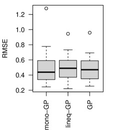
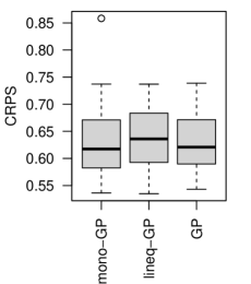
Figure 17: Metrics on the 1d logit MC experiment. Smaller is better for all.

In particular, although the ordinary GP cannot guarantee monotonicity, as shown in Figure 5, it nevertheless provides accurate predictions with good UQ. In fact, since it integrates over the latent field analytically its metrics have lower MC error (narrower boxplots). Mono-GP and lineq-GP both require MC integration, the accuracy of which is determined by a limited amount of posterior sampling.

B.2 Michalewicz deep GP comparison

Here we report on a MC experiment in the style of Section 5.2. Consider the “Michalewicz” function (VLSE; Surjanovic and Bingham,, 2013):

$$f(x)=-\sum_{i=1}^{p}\sin(x_{i})\sin^{2m}\left(\frac{ix_{i}^{2}}{\pi}\right),\quad\quad x\in[0,\pi]^{p}.$$

For variety, we ran our MC experiment in 3d ($p=3$) and set $m=10$, which is the recommended value. Inputs were coded to the unit cube and back-transformed as needed. Training/testing sets are generated from an LHS design with $(n,n^{\prime})=(100,1000)$.

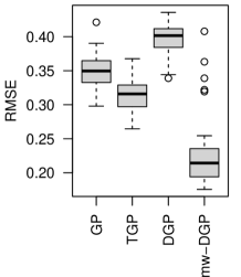
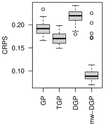
Figure 18: Michalewicz (3D) comparison.

Otherwise the setup is the same as our earlier DGP-based experiments. Results are shown in Figure 18. It is clear that mw-DGP outperforms the three other methods in terms of both accuracy and UQ. Interestingly, the ordinary GP does better than DGP. The extreme flexibility of a DGP may in fact may be a detriment to its performance without suitable regularization, e.g., as provided by mw-DGP. However, it is surely possible to engineer an example which is rotated along a diagonal that would thwart a purely axis-aligned process.

B.3 Timing comparisons

Here we measure fitting time on the 2d Lopez–Lopera [Section 4.2] and 3d Michalewicz [Appendix B.2] examples. Besides varying the training and testing set sizes commensurately ($n=n^{\prime}$), there are no other changes from those experiments. Prediction time is not reported because the additional expense represents less than 15% of computational time for all methods (and less than 1% for our method). We vary $n$ on an exponential schedule beginning with $n\approx 50$ and ending with $n\approx 8000$ for 2d Lopex–Lopera and $n\approx 2500$ for 3d Michalewicz.

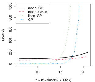
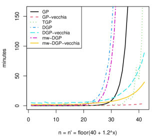
Figure 19: Compute times varying $n=n^{\prime}$ on 5d Lopez–Lopera (left) and 3d Michalewicz (right) examples from earlier.

Figure 19 shows the results. The $y$-axis on both plots is cut off to enhance visibility for the smaller-$n$ experiments. Focusing on the left panel first, notice that mono-GP is slower (both variations), relatively speaking, for these. But eventually the cubic costs of lineq-GP and the ordinary GP kick in, and those methods become prohibitively slow. Mono-GP and lineq-GP are similar on computation time for $n\approx 500$, with the ordinary GP being faster in that instance which we attribute to its more streamlined C implementation. The break even point for mono-GP and the ordinary GP is $n\approx 1000$. When $n\approx 3300$ mono-GP only takes 142 seconds, which is barely double the 71 seconds required for $n=31$. However, lineq-GP and the ordinary GP take 30000 and 2000 seconds respectively.

The variation labeled “mono-GP” uses R’s built-in approx, whereas “mono-GP-fo” uses the thriftier fo_approx. In other experiments not reported on here, we found that our bespoke fo_approx was 2–3x faster by pre-computing an appropriate indexing, as opposed to re-computing it each time it is needed. When situated within our mono-GP MCMC, which of course involves many other calculations, the speedup (shown in the figure) is a more modest but noticeable 50%. We use this “mono-GP-fo” as our default (i.e., for mono-GP) in the rest of the empirical work reported on in this paper.

On the 3d Michalewicz problem, some methods (e.g. DGP, mw-DGP) took hours, if not days, to complete for the larger training data sets without use of the Vecchia approximation. This is illustrated by the $y$-axis only extending to $\approx 2.5$ hours in the right panel of Figure 19. After $n>200$, there’s essentially no contest in terms of efficiency. But the use of a fixed grid size in mw-DGP also adds a speedup. At every training set size, mw-DGP runs faster than DGP. It’s the same story when the Vecchia approximation is employed for both methods. Perhaps more importantly, as the training set reaches sizes that are orders of magnitude larger, the gap between mw-DGP-vecchia and DGP-vecchia actually increases. This is because all operations on the warping layer in mw-DGP-vecchia use the fixed size grid, thereby locking in the cubic costs at $\mathcal{O}(n_{g}^{3})$. DGP-vecchia approximates the warping layer, so the computational costs still increase linearly as training set size grows.

TGP’s execution time is a little more variable, depending on the number of partitions it creates. Although it is able to handle larger training data than DGP, with execution time not spiking until $n\approx 700$, TGP still cannot match the efficiency of mw-DGP-vecchia for data of substantial size. It’s no surprise that GP-vecchia, without the addition of a warping layer (and the extra computation that accompanies it), executes in a smaller time frame than mw-DGP-vecchia. In fact, it is impossible for mw-DGP-vecchia to beat GP-vecchia, because they both perform the same approximation on the outer layer. But with that extra warping layer, mw-DGP-vecchia easily wins in RMSE and CRPS, as shown in 18.

B.4 Additional sensitivity visuals

We omitted the Lopez–Lopera arctan sensitivity plots in Section 4.2 to save space, so here they are in Figure 20. Each panel shows all saved posterior samples of $F_{n}^{\cdot,j}$ for $j=1,\dots,p=10$.

Figure 20: Latent functions for arctan example compared to the truth.

Observe that they are all quite similar in shape. In this example, the $\nu$-vector is key in weighting contributions from each individual input. In Figure 21 we show the posterior means of samples of $\nu^{(t)}\times F_{n}^{(t)}$, where each line corresponds to one of the columns of this matrix.

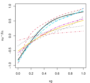
Figure 21: Sensitivity via posterior means of $\nu_{j}F_{n}^{\cdot j}$ on 10d Lopez–Lopera artcan example.

Observe that some of those lines span a wider swath of the $y$-axis, amplifying their contribution to the overall predictive mean through the additive model.

References

- Bachoc et al., (2022) Bachoc, F., López-Lopera, A. F., and Roustant, O. (2022). “Sequential construction and dimension reduction of Gaussian processes under inequality constraints.” SIAM Journal on Mathematics of Data Science, 4, 2, 772–800.
- Banerjee et al., (2004) Banerjee, S., Carlin, B., and Gelfand, A. (2004). Hierarchical Modeling and Analysis for Spatial Data. Chapman and Hall/CRC.
- Banerjee et al., (2008) Banerjee, S., Gelfand, A., Finley, A., and Sang, H. (2008). “Gaussian predictive process models for large spatial data sets.” Journal of the Royal Statistical Society: Series B (Statistical Methodology), 70, 4, 825–848.
- Booth, (2024) Booth, A. S. (2024). deepgp: Bayesian Deep Gaussian Processes using MCMC. R package version 1.1.3.
- Bui et al., (2016) Bui, T., Hernández-Lobato, D., Hernandez-Lobato, J., Li, Y., and Turner, R. (2016). “Deep Gaussian processes for regression using approximate expectation propagation.” In International conference on machine learning, 1472–1481. PMLR.
- Cole et al., (2021) Cole, D. A., Christianson, R. B., and Gramacy, R. B. (2021). “Locally induced Gaussian processes for large-scale simulation experiments.” Statistics and Computing, 31, 3, 1–21.
- Cutajar et al., (2017) Cutajar, K., Bonilla, E. V., Michiardi, P., and Filippone, M. (2017). “Random feature expansions for deep Gaussian processes.” In International Conference on Machine Learning, 884–893. PMLR.
- Damianou and Lawrence, (2013) Damianou, A. and Lawrence, N. D. (2013). “Deep Gaussian processes.” In Artificial intelligence and statistics, 207–215. PMLR.
- Gelman et al., (1995) Gelman, A., Carlin, J. B., Stern, H. S., and Rubin, D. B. (1995). Bayesian data analysis. Chapman and Hall/CRC.
- Genz and Bretz, (2009) Genz, A. and Bretz, F. (2009). Computation of Multivariate Normal and t Probabilities. Lecture Notes in Statistics. Heidelberg: Springer-Verlag.
- Gneiting and Raftery, (2007) Gneiting, T. and Raftery, A. E. (2007). “Strictly proper scoring rules, prediction, and estimation.” Journal of the American statistical Association, 102, 477, 359–378.
- Gramacy and Lee, (2008) Gramacy, R. and Lee, H. (2008). “Bayesian treed Gaussian process models with an application to computer modeling.” Journal of the American Statistical Association, 103, 483, 1119–1130.
- Gramacy, (2007) Gramacy, R. B. (2007). “tgp: An R Package for Bayesian Nonstationary, Semiparametric Nonlinear Regression and Design by Treed Gaussian Process Models.” Journal of Statistical Software, 19, 9, 1–46.
- Gramacy, (2016) — (2016). “laGP: Large-Scale Spatial Modeling via Local Approximate Gaussian Processes in R.” Journal of Statistical Software, 72, 1, 1–46.
- Gramacy, (2020) — (2020). Surrogates: Gaussian Process Modeling, Design and Optimization for the Applied Sciences. Boca Raton, Florida: Chapman Hall/CRC. http://bobby.gramacy.com/surrogates/.
- Gramacy and Lee, (2009) Gramacy, R. B. and Lee, H. K. H. (2009). “Adaptive Design and Analysis of Supercomputer Experiments.” Technometrics, 51, 2, 130–145.
- Gramacy and Taddy, (2010) Gramacy, R. B. and Taddy, M. (2010). “Categorical Inputs, Sensitivity Analysis, Optimization and Importance Tempering with tgp Version 2, an R Package for Treed Gaussian Process Models.” Journal of Statistical Software, 33, 6, 1–48.
- Hoff, (2009) Hoff, P. D. (2009). A first course in Bayesian statistical methods, vol. 580. Springer.
- Katzfuss and Guinness, (2021) Katzfuss, M. and Guinness, J. (2021). “A general framework for Vecchia approximations of Gaussian processes.” Statistical Science, 36, 1, 124–141.
- Laradji et al., (2019) Laradji, I. H., Schmidt, M., Pavlovic, V., and Kim, M. (2019). “Efficient deep Gaussian process models for variable-sized inputs.” In 2019 International Joint Conference on Neural Networks (IJCNN), 1–7. IEEE.
- López-Lopera et al., (2022) López-Lopera, A., Bachoc, F., and Roustant, O. (2022). “High-dimensional additive Gaussian processes under monotonicity constraints.” Advances in Neural Information Processing Systems, 35, 8041–8053.
- Lopez-Lopera, (2022) Lopez-Lopera, A. F. (2022). lineqGPR: Gaussian Process Regression with Linear Inequality Constraints. R package version 0.3.0.
- Marrel et al., (2009) Marrel, A., Iooss, B., Laurent, B., and Roustant, O. (2009). “Calculations of Sobol indices for the Gaussian process metamodel.” Reliability Engineering & System Safety, 94, 3, 742–751.
- McKay et al., (2000) McKay, M. D., Beckman, R. J., and Conover, W. J. (2000). “A comparison of three methods for selecting values of input variables in the analysis of output from a computer code.” Technometrics, 42, 1, 55–61.
- Mehta et al., (2014) Mehta, P. M., Walker, A., Lawrence, E., Linares, R., Higdon, D., and Koller, J. (2014). “Modeling satellite drag coefficients with response surfaces.” Advances in Space Research, 54, 8, 1590–1607.
- Murray et al., (2010) Murray, I., Adams, R. P., and MacKay, D. J. C. (2010). “Elliptical slice sampling.” In The Proceedings of the 13th International Conference on Artificial Intelligence and Statistics, vol. 9 of JMLR: W&CP, 541–548. PMLR.
- Oakley and O’Hagan, (2004) Oakley, J. and O’Hagan, A. (2004). “Probabilistic sensitivity analysis of complex models: a Bayesian approach.” Journal of the Royal Statistical Society: Series B (Statistical Methodology), 66, 3, 751–769.
- Paciorek and Schervish, (2003) Paciorek, C. and Schervish, M. (2003). “Nonstationary covariance functions for Gaussian process regression.” Advances in neural information processing systems, 16.
- Paciorek and Schervish, (2006) — (2006). “Spatial modelling using a new class of nonstationary covariance functions.” Environmetrics: The Official Journal of the International Environmetrics Society, 17, 5, 483–506.
- Pamadi et al., (2004) Pamadi, B., Covell, P., Tartabini, P., and Murphy, K. (2004). “Aerodynamic characteristics and glide-back performance of langley glide-back booster.” In 22nd Applied Aerodynamics Conference and Exhibit, 5382.
- Rasmussen and Williams, (2006) Rasmussen, C. and Williams, C. (2006). Gaussian Processes for Machine Learning. Cambridge, MA: MIT Press.
- Riihimäki and Vehtari, (2010) Riihimäki, J. and Vehtari, A. (2010). “Gaussian processes with monotonicity information.” In Proceedings of the thirteenth international conference on artificial intelligence and statistics, 645–652. JMLR Workshop and Conference Proceedings.
- Salimbeni and Deisenroth, (2017) Salimbeni, H. and Deisenroth, M. (2017). “Doubly stochastic variational inference for deep Gaussian processes.” arXiv preprint arXiv:1705.08933.
- Saltelli et al., (2000) Saltelli, A., Chan, K., and Scott, M. (2000). Sensitivity Analysis. New York, NY: John Wiley & Sons.
- Sampson and Guttorp, (1992) Sampson, P. D. and Guttorp, P. (1992). “Nonparametric estimation of nonstationary spatial covariance structure.” Journal of the American Statistical Association, 87, 417, 108–119.
- Santner et al., (2018) Santner, T., Williams, B., and Notz, W. (2018). The Design and Analysis of Computer Experiments, Second Edition. New York, NY: Springer–Verlag.
- Sauer et al., (2023a) Sauer, A., Cooper, A., and Gramacy, R. B. (2023a). “Non-stationary Gaussian process surrogates.” arXiv preprint arXiv:2305.19242.
- Sauer et al., (2023b) — (2023b). “Vecchia-approximated deep Gaussian processes for computer experiments.” Journal of Computational and Graphical Statistics, 32, 3, 824–837.
- Sauer et al., (2023c) Sauer, A., Gramacy, R. B., and Higdon, D. (2023c). “Active learning for deep Gaussian process surrogates.” Technometrics, 65, 1, 4–18.
- Schmidt and O’Hagan, (2003) Schmidt, A. M. and O’Hagan, A. (2003). “Bayesian inference for non-stationary spatial covariance structure via spatial deformations.” Journal of the Royal Statistical Society: Series B (Statistical Methodology), 65, 3, 743–758.
- Snelson and Ghahramani, (2006) Snelson, E. and Ghahramani, Z. (2006). “Sparse Gaussian processes using pseudo-inputs.” In Advances in Neural Information Processing Systems, 1257–1264.
- Sun et al., (2019) Sun, F., Gramacy, R. B., Haaland, B., Lawrence, E., and Walker, A. (2019). “Emulating satellite drag from large simulation experiments.” SIAM/ASA Journal on Uncertainty Quantification, 7, 2, 720–759.
- Surjanovic and Bingham, (2013) Surjanovic, S. and Bingham, D. (2013). “Virtual library of simulation experiments: test functions and datasets.” http://www.sfu.ca/~ssurjano.
- Tran et al., (2023) Tran, A., Maupin, K., and Rodgers, T. (2023). “Monotonic Gaussian process for physics-constrained machine learning with materials science applications.” Journal of Computing and Information Science in Engineering, 23, 1, 011011.
- Ustyuzhaninov et al., (2020) Ustyuzhaninov, I., Kazlauskaite, I., Ek, C. H., and Campbell, N. (2020). “Monotonic gaussian process flows.” In International Conference on Artificial Intelligence and Statistics, 3057–3067. PMLR.
- Wu et al., (2022) Wu, L., Pleiss, G., and Cunningham, J. (2022). “Variational Nearest Neighbor Gaussian Processes.” arXiv preprint arXiv:2202.01694.
- Wycoff, (2023) Wycoff, N. (2023). “Surrogate Active Subspaces for Jump-Discontinuous Functions.”
- Zammit-Mangion et al., (2022) Zammit-Mangion, A., Ng, T. L. J., Vu, Q., and Filippone, M. (2022). “Deep compositional spatial models.” Journal of the American Statistical Association, 117, 540, 1787–1808.