3D $\mathcal{N}=1$ supergravity from Virasoro TQFT: Gravitational partition function and Out-of-time-order correlator

Abstract

In this paper, we compute the partition functions of $\mathcal{N}=1$ SUGRA for different boundary topologies, i.e. sphere and torus, using super-Virasoro TQFT. We use fusion and modular kernels of the super-Liouville theory to compute the necklace-channel conformal block and showcase formalism by proving that the inner product holds for superconformal blocks, defined as states in the Hilbert space. Finally, we compute the out-of-time-order correlator out-of-time-order correlator for the torus topology with superconformal primary insertions as matter using the tools of super-Virasoro TQFT and investigate its early-time behaviour.

1 Introduction

Quantum gravity has been a topic of interest for many years. However, the construction of tractable problems in quantum gravity is non-trivially challenging, with much development occurring in the lower dimensional cases Jackiw:1984je ; Teitelboim:1983ux ; Saad:2019lba . Also, several insights came from the AdS/CFT correspondence Maldacena:1997re ; Witten:1998qj . In the last few years, many studies on computing the partition function for two-dimensional gravity and its deformation have been made Saad:2019lba ; Turiaci:2023jfa ; Iliesiu:2019lfc ; Iliesiu:2020qvm ; Iliesiu:2020zld ; Collier:2023cyw ; Ebert:2022gyn ; Bhattacharyya:2023gvg . However, the portrait of a richer three-dimensional gravity is still not very clear. In three spacetime dimensions, pure Einstein gravity is non-dynamical, implying the non-existence of gravitational waves. This simplifies the gravity theory dramatically and provides a hint that gravity theory in three dimensions can be formulated in terms of topological quantum field theory (TQFT) Atiyah:1989vu ; Mikhaylov:2017ngi , where the edge modes are in the form of the graviton excitations in the asymptotic boundaries. However, full quantum treatment of three-dimensional gravity did not achieve much progress, unlike two-dimensional Jackiw-Titelboim gravity Saad:2019lba . Though the ensemble average description works well in the case of JT gravity, in the case of 3d gravity there are strong constraints of locality in terms of operator product expansion and modular transformations. The solution to the crossing equations in the holographic regime is rarely available to us. There have been multiple efforts of quantizing three-dimensional gravity Maloney:2007ud ; Yin:2007gv ; Witten:2007kt ; Manschot:2007zb have emerged since the late 2000s based on AdS/CFT conjecture Maldacena:1997re . Despite significant progress, the status of dual boundary CFT is not yet fully settled. Taking intuition from two-dimensional gravity Saad:2019lba , it is expected that the boundary CFT is not just a family of 2D CFTs admitting a large-c limit but an ensemble of chaotic large-c CFTs. In spite of partial progress on this line Maloney:2020nni ; Collier:2021rsn ; Afkhami-Jeddi:2020ezh ; Benjamin:2021wzr ; Chandra:2022bqq ; Belin:2020hea ; Mertens:2022ujr ; Eberhardt:2019ywk ; Eberhardt:2018ouy , there is no known unitary large-c chaotic CFT with a sparse light spectrum and Virasoro symmetry. Recently, the problem has been nicely tackled in Collier:2023fwi ; Collier:2024mgv showing the relation of $AdS_{3}$ quantum gravity with topological field theory, which relies on the bulk description of the problem, unlike the other conventional approaches, and opens up a new pathway to computing observables directly from the bulk description. These issues are further addressed in Dymarsky:2024frx ; deBoer:2024kat ; Jafferis:2024jkb .

In this paper, we aim to address the quantization of $\mathcal{N}=1$ supergravity Ducrocq:2021vkh via geometric quantization using super-Virasoro TQFT. The TQFT description for pure $AdS_{3}$ gravity has been studied for decades, starting from the matching at the classical level between $PSL(2,\mathbb{R})\times PSL(2,\mathbb{R})$ Chern-Simons theory Einstein’s gravity in $AdS_{3}$. However, the direct quantization $PSL(2,\mathbb{R})\times PSL(2,\mathbb{R})$ Chern-Simmons theory is not the same as quantizing pure $AdS_{3}$ gravity. The fundamental principles in gravity need the metric to be non-degenerate, while the CS theory does not have such a requirement. The gravitational phase decomposes to two copies of Teichmuller space on a spatial slice (say $\Sigma$). Teichmuller space describes the shape of the initial value surface and becomes the universal covering of the moduli space of Riemann surfaces. For a Riemann surface $\Sigma_{g,n}$ of genus $g$ and $n$ punctures, the Teichmuller space $\mathcal{T}_{g,n}$ can also be understood as the space of all metrics on $\Sigma_{g,n}$ modulo small diffeomorphisms and Weyl rescalings Eberhardt:2023mrq ,

$$\mathcal{T}_{g,n}=\frac{\text{Metrics on }\Sigma_{g,n}}{\text{Diff}_{0}(\Sigma_{g,n})\times\text{Weyl}(\Sigma_{g,n})}.$$ (1)

The important fact here is that the Teichmuller space can be quantized on its own, and therefore, it is possible to assign a Hilbert space $H_{\Sigma}$ having a definition of well-defined inner-product. Quantum Teichmuller theory has been an intriguing topic connecting various branches of mathematics and physics Atiyah:1989vu ; EllegaardAndersen:2011vps ; Mikhaylov:2017ngi ; Collier:2023fwi . There are many generalizations possible for the Teichmuller TQFT, especially considering moduli spaces of super Riemann surfaces. Though the super Teichmuller space plays a fundamental role in superstring perturbation theory, geometric quantization is a relatively new direction. The main goal of the paper is to generalize the technologies of geometric quantization Eberhardt:2023mrq for the supersymmetric case. Sometimes it is also referred to as super-Teichmuller spin TQFT Aghaei:2015bqi ; Aghaei:2020otq in literature. In this paper, we compute the partition functions of different 3-manifolds. Here, the algorithm is based on surgery techniques Sen:2024nfd of super-Riemann surfaces Witten:2012ga . It turns out that the super-Teichmuller TQFT is connected to the three-dimensional Chern-Simmons theory with complexifications of $OSp(1|2)$ and $SO(3)$ gauge groups.

In the process of geometric quantization, we identified the states in the bulk Hilbert space with superconformal blocks. Conformal blocks Dolan:2000ut are known to be the solution of the Casimir equation for the corresponding conformal group. For $\mathcal{N}=1$ super-Liouville theory, we systematically establish the inner product of conformal blocks following Eberhardt:2023mrq . The inner product turns out to produce a Dirac delta function with the difference of two different Wilson line momenta. The $\mathcal{N}=1$ super-Liouville theory has contributions from fermions leading to the choice of different spin structures in the super-Riemann surface. Depending on the different boundary conditions of the super-torus geometry, we have to perform different modular sums, which are given in terms of the famous Eisenstein series representation. Apart from this, the spin structures using Kasteleyn orientations are known for $\mathcal{N}=1$ Aghaei:2020otq . The isometry group OSp(1|2) acts on the upper half-plane $\mathbb{H}^{1|1}$ by general Möbius transformations of the form,

$$\begin{split}&x\rightarrow x^{\prime}=\frac{ax+b+\rho\theta}{cx+d+\delta\theta},\leavevmode\nobreak\ \leavevmode\nobreak\ \leavevmode\nobreak\ \leavevmode\nobreak\ \leavevmode\nobreak\ \theta\rightarrow\theta^{\prime}=\frac{\alpha x+\beta+g\theta}{cx+d+\delta\theta}.\end{split}$$ (2)

We can define two types of conformal invariants, even Z and odd $\zeta$ under the general Möbius transformation. The former is the superconformal generalization of the normal cross ratio in the super upper half-plane for points $P_{j}=(x_{j}|\theta_{j})$, $j=1,\cdots 4$:

$$Z:=\frac{X_{14}X_{23}}{X_{12}X_{34}},$$

where $X_{ij}:=x_{i}-x_{j}-\theta_{i}\theta_{j}$. The other odd invariant cross ratio $\zeta$ for the collection of three points $P_{j}=(x_{j}|\theta_{j})$, $j=1,\cdots 3$:

$$\zeta:=\pm\frac{x_{23}\theta_{1}+x_{31}\theta_{2}+x_{12}\theta_{3}-\frac{1}{2}\theta_{1}\theta_{2}\theta_{3}}{(X_{12}X_{23}X_{31})^{1/2}},$$ (3)

where, $x_{ij}:=x_{i}-x_{j}$.

The field of quantum chaos Larkin1969QuasiclassicalMI ; Haake:2010fgh , developed in the early seventies, addresses the quantum manifestation of classically chaotic systems. There are many studies aiming to probe the quantum chaotic nature of quantum many-body systems have been done Bohigas:1983er ; Berry ; DAlessio:2015qtq ; Hosur:2015ylk ; Nahum:2017yvy ; vonKeyserlingk:2017dyr ; Aleiner:2016eni ; Garttner:2016mqj ; syk ; Maldacena:2016hyu ; Cotler:2017jue ; Chowdhury:2017jzb ; khemani:2018sdn ; Seshadri:2018yya ; Hashimoto:2017oit ; Ali:2019zcj ; Bhattacharyya:2020art . The study of quantum chaos in quantum gravity and holography has seen a renewed interest in recent years Sachdev1992GaplessSG ; DiFrancesco:1993cyw ; Roberts:2014ifa ; Maldacena:2015waa ; Maldacena:2016hyu ; Kitaev:2017awl ; syk ; Garcia-Garcia:2016mno ; Papadodimas:2015xma ; Sarosi:2017ykf ; Cotler:2016fpe ; Balasubramanian:2016ids ; Krishnan:2016bvg ; Dyer:2016pou . The gap between the two apparently distinct fields has been bridged in Roberts:2014ifa ; Altland:2022xqx , focusing on the 2D quantum gravity. Over the years, several diagnostics have been developed to probe quantum chaos Bhattacharyya:2019txx ; Kudler-Flam:2019kxq . In particular, to probe the early-time (quantum) chaos, one computes the out-of-time-order correlator (OTOC) Zhou:2021syv ; Swingle:2018ekw ; Shenker:2013pqa ; Roberts:2014ifa ; Maldacena:2015waa ; Stanford:2015owe ; Mertens:2022irh . One of the primary focuses of our study in this paper, is the OTOC of the form,

$$\langle\mathcal{O}_{A}\mathcal{O}_{B}\mathcal{O}_{A}\mathcal{O}_{B}\rangle_{\beta}$$

on a torus. Here $\beta$ is the inverse temperature. $\mathcal{O}_{A}$ and $\mathcal{O}_{B}$ are approximately local insertions smeared over the thermal circle. The behaviour of such functions should be contrasted with the behaviour of correlation functions of the following type,

$$\langle\mathcal{O}_{A}(t)\mathcal{O}_{A}(t)\mathcal{O}_{B}\mathcal{O}_{B}\rangle_{\beta},\leavevmode\nobreak\ \leavevmode\nobreak\ \leavevmode\nobreak\ \leavevmode\nobreak\ \langle\mathcal{O}_{A}\mathcal{O}_{B}(t)\mathcal{O}_{B}(t)\mathcal{O}_{A}\rangle_{\beta}$$

which tends to a $\mathcal{O}(1)$ value $\langle\mathcal{O}_{A}\mathcal{O}_{A}\rangle_{\beta}\langle\mathcal{O}_{B}\mathcal{O}_{B}\rangle_{\beta}$ as $t$ increases. All of the above four-point configurations can be obtained from the Euclidean four-point function. The difference in behaviour arises due to analytic continuation and multivaluedness of a function. OTOCs have been well studied in the literature, particularly for 2D CFTs Roberts:2014ifa ; Kusuki:2019gjs ; Caputa:2017rkm ; Caputa:2016tgt ; Craps:2021bmz ; Das:2022jrr . One can extract the quantum Lyapunov exponent from the early-time exponential decay of the OTOC and for certain holographic theories (at finite temperature) it satisfies the Maldacena-Shenker-Stanford (MSS) bound Maldacena:2015waa . Also, by investigating the delay of early-time exponential delay of OTOC, one can extract the information about scrambling time Hosur:2015ylk . It is worth noting that black holes are fast scramblers, i.e scrambling time scales logarithmically in the number of degrees of freedom of the system, $t_{Sc}\sim\log\,N$ Sekino:2008he . Motivated by these, in this paper, to probe the chaotic nature of the bulk gravitational theory, we compute the leading contribution to the OTOC from the superconformal matter insertions on the super-torus using the formalism of the Virasoro-TQFT. We will restrict ourselves to the large-$c$ regime in $\mathcal{N}=1$ superconformal field theory to connect with the gravitational case.

Our paper is organized as follows. In Sec. (2), we start by reviewing $\mathcal{N}=1$ super-Liouville theory, and subsequently, we describe the ingredients for computing the partition function for wormholes with different number of boundaries and topologies using super-Teichmuller TQFT. Furthermore, we discuss the process of geometric quantization for super-Liouville theory and the inner product of superconformal blocks. In Sec. (3), we calculated the (super-) VTQFT partition and the gravitational partition function by taking some specific examples of topologies. Then, in Sec. (4), we put the calculation of 4-point superconformal blocks on the torus, which is required to compute the OTOC. Finally, in Sec. (5), to probe the regime of chaos, we calculate the out-of-time-order correlation functions with super-Liouville matter insertions. To get an analytic handle on it, we calculate it using some specific but relevant limits. We use braiding and modular transformations to compute the OTOC in both channels, i.e. the necklace and the OPE channel. In Sec. (6), we conclude by summarising the main findings and giving some future outlooks. Last but not least, we have added a few appendices to give the details of some of the computations.

Some Definition:

•  Modular parameter $\tau$ is related to $q$ as $q=e^{2\pi i\tau}\,.$
•  $\,\Theta(\tau)$ are Mock theta functions .
•   $\chi_{NS}$ are super-virasoro characters .
•   $\xi(z,\theta)$ are super-elliptic functions .
•   $(a)_{m}$ denotes the Pochhammer symbols, $(a)_{m}=:\frac{\Gamma(a+m)}{\Gamma(a)}\,.$
•   $s\mathcal{T}\equiv$ super-Teichmuller .

2 Geometric quantization and inner product of super conformal blocks

In this section, we will discuss how to compute the gravitational partition function using the super-Teichmuller spin TQFT, the boundary theory being the $\mathcal{N}=1$ super-Liouville theory. The gravitational partition function is found from the character of the $\textrm{{\bf Osp}}(1|2)$ algebra. The gravitational partition function can also be given by the square of the super-Liouville partition function as shown in Eberhardt:2023mrq . We claim that the inner product of the super-Liouvile zero-point conformal block on the torus is, gray!8 black

$$\begin{split}\tikzmarkin[disableroundedcorners=true]{e22}(0.5,-0.5)(-0.1,0.8)\langle\mathcal{F}^{s(0)}_{(1,0)}(\vec{P}_{1})|\mathcal{F}^{s(0)}_{(1,0)}(\vec{P}_{2})\rangle=\int_{\mathcal{T}}d(\textrm{sWP})\leavevmode\nobreak\ {\textrm{sdet}}(\hat{\mathcal{P}}_{1}^{\dagger}\hat{\mathcal{P}}_{1})^{1/2}\leavevmode\nobreak\ Z_{\text{timelike SL}}\,\mathcal{F}^{s(0)}_{(1,0)}(\vec{P}_{2})\overline{\mathcal{F}^{s(0)}_{(1,0)}}(\vec{P}_{1})\propto{\delta(\vec{P_{1}}-\vec{P_{2}})}.\tikzmarkend{e22}\end{split}$$ (4)

where, $\mathcal{F}^{s(\ell)}_{(g,n)}(\vec{P})$ is the $\ell$-point super-conformal block for Riemann surface with $g$-genus and $n$-puncture, $P$ denotes the Liouville momenta , sWP is called the super-Weil-Peterson volume and sdet is the super-determinant. In this section, we wish to prove our claim. However, before we get into the details of our proof, let us take a detour to briefly review the necessary concepts utilised in this section.

A brief review of super-Liouville Theory

Let us review the basics of the $\mathcal{N}=1$ super-Liouville theory. The theory is defined via following Lagrangian density Poghossian:1996agj ,

$$\mathcal{L}=\frac{1}{2}g_{ab}\partial_{a}\phi\partial_{b}\phi+\frac{1}{2\pi}(\psi\bar{\partial}\psi+\bar{\psi}\partial\bar{\psi})+2i\mu b^{2}\bar{\psi}\psi e^{b\phi}+2\pi\mu^{2}b^{2}e^{2b\phi}\,.$$ (5)

The energy-momentum tensor and the supercurrent is given by,

$$\begin{split}&T=-\frac{1}{2}(\partial\phi\partial\phi-Q\partial^{2}\phi+\psi\partial\psi)\,,\\ &G=i(\psi\partial\phi-Q\partial\psi)\,.\end{split}$$ (6)

The superconformal algebra is given by,

$$\begin{split}&[L_{m},L_{n}]=(m-n)L_{m+n}+\frac{c_{SL}}{12}m(m^{2}-1)\delta_{m+n},\\ &[L_{m},G_{k}]=\frac{m-2k}{2}{G_{m+k}},\\ &\{G_{k},G_{l}\}=2L_{l+k}+\frac{c}{3}(k^{2}-\frac{1}{4})\delta_{k+l}\,.\end{split}$$ (7)

Here the central charge is given by $c_{SL}=\frac{3}{2}+3Q^{2}$ where $Q=b+\frac{1}{b}.$ $k,l$ takes integer values for the Ramond algebra, and half-integer ones for Neveu-Schwarz (NS) algebra. $Q$ is known as the total background charge.

For the Liouville theory, one-point function of the vertex operator on a torus is given by Artemev:2022sfi ,

$$\langle V_{a}\rangle_{\tau}=\int_{\gamma}\frac{dP}{4\pi}C^{(L)Q/2+iP}_{a,Q/2+iP}(q\bar{q})^{-1/24+P^{2}}\times|F_{L}(\Delta_{a}^{L},\Delta^{L}_{Q/2+iP},q)|^{2}$$

where the structure constant is given by,

$$C^{(L)Q/2+iP}_{a,Q/2+iP}=(\pi\mu\gamma(b^{2})b^{2-2b^{2}})^{-a/b}\frac{\Upsilon(b)\Upsilon(2a)\Upsilon(2iP)\Upsilon(-2iP)}{\Upsilon^{2}(a)\Upsilon(a+2iP)\Upsilon(a-2iP)}$$ (8)

and $F_{L}$ is the conformal block. The $\Upsilon(x)$ functions are defined as,

$$\begin{split}&\Upsilon_{b}(x)=\frac{1}{\Gamma_{b}(x)\Gamma_{b}(Q-x)},\leavevmode\nobreak\ \leavevmode\nobreak\ \leavevmode\nobreak\ \leavevmode\nobreak\ \leavevmode\nobreak\ \leavevmode\nobreak\ \leavevmode\nobreak\ \leavevmode\nobreak\ S_{b}(x)=\frac{\Gamma_{b}(x)}{\Gamma_{b}(Q-x)}\,,\\ &\Gamma_{NS}(x)=\Gamma_{b}(x/2)\,\Gamma_{b}(\frac{x+Q}{2}),\leavevmode\nobreak\ \leavevmode\nobreak\ \leavevmode\nobreak\ \Gamma_{R}(x)=\Gamma_{b}(\frac{x+b}{2})\Gamma_{b}(\frac{x+b^{-1}}{2})\,,\\ &\Upsilon_{NS}(x)=\Upsilon_{b}(x/2)\,\Upsilon_{b}(\frac{x+Q}{2})\,,\leavevmode\nobreak\ \leavevmode\nobreak\ \Upsilon_{R}(x)=\Upsilon_{b}(\frac{x+b}{2})\Upsilon_{b}(\frac{x+b^{-1}}{2}).\end{split}$$ (9)

Using the following definition of the superfields,

$$\Phi_{a}=\phi_{a}(z,\bar{z})+\theta\psi_{a}(z,\bar{z})-\bar{\theta}\bar{\psi}_{a}(z,\bar{z})\,,$$

we can write the two-point and three-point functions in the following way,

$$\langle\Phi_{1}(Z_{1},\bar{Z}_{1})\Phi_{2}(Z_{2},\bar{Z}_{2})\rangle=\frac{c_{12}}{Z_{12}^{2\Delta}\bar{Z}_{12}^{2\bar{\Delta}}},\,\,\,\,\,\,\,\Delta=\Delta_{1}=\Delta_{2},\,\,\,\bar{\Delta}=\bar{\Delta}_{1}=\bar{\Delta}_{2}\,.$$ (10)

Here $c_{12}$ is a constant, and

$$\begin{split}\langle\Phi(z_{3},\theta_{3};\bar{z}_{3},\bar{\theta}_{3})\Phi(z_{2},\theta_{2};\bar{z}_{2},\bar{\theta}_{2})\Phi(z_{1},\theta_{1};\bar{z}_{1},\bar{\theta}_{1})\rangle&=Z_{32}^{\beta_{1}}Z_{31}^{\beta_{2}}Z_{21}^{\beta_{3}}\\ &\,\langle\Phi(\infty,0;\infty,0)\Phi(1,\Theta;1,\bar{\Theta})\Phi(0,0;0,0)\rangle\end{split}$$ (11)

where,

$$\beta_{i}=\Delta_{i}-\Delta_{j}-\Delta_{k},\leavevmode\nobreak\ Z_{12}=z_{1}-z_{2}-\theta_{1}\theta_{2},\leavevmode\nobreak\ \Theta=\frac{1}{\sqrt{z_{12}z_{13}z_{23}}}\Big{(}\theta_{1}z_{23}+\theta_{2}z_{31}+\theta_{3}z_{12}-\frac{1}{2}\theta_{1}\theta_{2}\theta_{3}\Big{)}\,.$$

We used conformal invariance to write the three-point function (11).

Geometric quantization in Liouville theory

Before proceeding to prove (4), we briefly review the geometric quantization technique in the context of the Liouville theory. To carry out the path integral over metric, we parametrize the space of metrics by $g={\color[rgb]{0,0,0}\exp(\delta v)e^{2\sigma}\hat{g}}$. Here $\hat{g}$ is transversal to the orbits of $\textrm{Weyl}(M)$ and $\textrm{Diff}_{0}(M)$. The joint action of the reparametrizations and Weyl transformations is given by DHoker:1988pdl ,

$$\delta g_{mn}=(2\delta\sigma+\nabla^{p}\delta v_{p})g_{mn}+(\mathcal{P}_{1}\delta v)_{mn}.$$ (12)

If the diffeomorphisms are generated by a vector field $v$, then

$$(\mathcal{P}_{1}v)_{mn}=\nabla_{m}v_{n}+\nabla_{n}v_{m}-(\nabla_{c}v^{c})g_{mn}\,.$$ (13)

$\mathcal{P}_{1}$ generates symmetric and traceless variations. Deformations $\delta g^{\perp}$ that are elements of $\textrm{Ker}\mathcal{P}_{1}^{\dagger}$ (satisfying $\mathcal{P}_{1}^{\dagger}\delta g^{\perp}=0$) are orthogonal to those generated by conformal transformations and Diffeomorphism.

$$\langle\delta g^{\perp},\mathcal{P}_{1}\vec{v}\rangle=\langle\mathcal{P}_{1}^{\dagger}\delta g^{\perp},\mathcal{P}_{1}\vec{v}\rangle=0\,.$$ (14)

Therefore, only those that are not achieved by diffeomorphism and Weyl transformation are inside the ($\textrm{Range}\mathcal{P}_{1})^{\perp}$. So any deformation can be decomposed into the following,

$$\Big{\{}\delta g_{mn}\Big{\}}=\Big{\{}{\bf\delta\sigma}g_{mn}\Big{\}}\bigoplus\textrm{Range}\,{\bf\mathcal{P}_{1}}\bigoplus Ker{\bf\mathcal{P}_{1}^{\dagger}},$$ (15)

where the action of $\mathcal{P}_{1}^{\dagger}$ on the symmetric tensors are given by,

$$(\mathcal{P}_{1}^{\dagger}\delta g)_{m}=-2\nabla^{n}\delta g_{mn},$$ (16)

and we have the following identification

$$(\textrm{Range}\,\mathcal{P}_{1})^{\perp}=\textrm{Kernel}\,\mathcal{P}_{1}^{\dagger}\,.$$ (17)

To determine the number of zero modes of the operators, one needs to resort to an index theorem, which gives the difference between the number of zero modes of the operator and its adjoint, expressing it in terms of a topological invariant. The index theorem reduces to the Riemann-Roch theorem BSMF_1958__86__97_0 , which says;

$$\dim(\textrm{Ker}\mathcal{P})-\,\dim(\textrm{Ker}\mathcal{P}^{\dagger})=3\chi(M)\,.$$ (18)

In the absence of the anomalies, the path integrals should reduce over the space of inequivalent metrics under the Weyl and diffeomorphism symmetries DHoker:1988pdl . Now, we proceed to write the path integral measure using the formulas for the bosonic string theory,

$$\begin{split}&\Bigg{(}\frac{\textrm{det}\mathcal{P}_{1}^{\dagger}\mathcal{P}_{1}}{\textrm{det}\langle\phi_{j}|\phi_{k}\rangle}\Bigg{)}^{1/2}=\Bigg{(}\frac{\textrm{det}\hat{\mathcal{P}}_{1}^{\dagger}\hat{\mathcal{P}}_{1}}{\textrm{det}\langle\hat{\phi}_{j}|\hat{\phi}_{k}\rangle}\Bigg{)}^{1/2}e^{-26S_{L}(\sigma)}\,,\\ &\Bigg{(}\frac{8\pi^{2}\textrm{det}^{\prime}\Delta_{g}}{d^{2}\xi\sqrt{g}}\Bigg{)}^{1/2}=\Bigg{(}\frac{8\pi^{2}\textrm{det}^{\prime}\Delta_{\hat{g}}}{d^{2}\xi\sqrt{\hat{g}}}\Bigg{)}^{1/2}e^{-S_{L}(\sigma)}\,.\end{split}$$ (19)

Now to compute the measure due to the change of variable from $g\rightarrow\{\sigma,v,\hat{g}\},$ we need to compute the Jacobian in the following way,

$$Dg_{mn}=\textrm{Vol}_{g}(g\delta\sigma,P_{1}\delta v,f_{j})\,D\sigma\,Dv\,dm_{j}\,.$$ (20)

In equation (20) we have used the fact,

$$\delta g(m)=\sum_{j=1}^{3h-3}\delta m_{j}\hat{f}_{j}\,.$$ (21)

Here, the coordinates along $\hat{S}$ are $\delta\sigma\hat{g},\hat{\mathcal{P}}_{1}\delta v$ and $f_{j}$. Using the orthogonality, the volume can be decomposed as DHoker:1988pdl ,

$$Dg_{mn}=\text{Vol}_{g}(g\delta\sigma)\,\text{Vol}_{g}(\mathcal{P}_{1}\delta v)\,\text{Vol}_{g}(f_{j}\perp\textrm{Proj. Ker}\,\mathcal{P}_{1}^{\dagger})\,D\sigma Dvdm_{j}$$ (22)

where one can define, $\text{Vol}_{g}(\mathcal{P}_{1}\delta v):={(\textrm{det}(\mathcal{P}_{1}^{\dagger}P_{1}))^{1/2}}$ and $\text{Vol}_{g}(f_{j}\perp\textrm{Proj}.\textrm{Ker}\mathcal{P}_{1}^{\dagger}):=\frac{\textrm{det}\langle f_{j}|\phi_{k}\rangle_{g}}{(\textrm{det}\langle\phi_{j}|\phi_{k}\rangle)^{1/2}_{g}}.$
Using ultralocality, the first term can be ignored. Again,

$$\langle f_{j}|\phi_{k}\rangle_{g}=\langle\hat{f}_{j}|\phi_{k}\rangle_{g}=\langle\mu_{j}|\phi_{k}\rangle_{g},$$

where, $\mu^{z}_{j\bar{z}}=\hat{g}^{z\bar{z}}\hat{f}_{jz\bar{z}}$ are the Beltrami differentials Baulieu:1987jz corresponding to the moduli deformations along the slice $\hat{S}$. Now we proceed to write the inner product of the states in the Teichmuller space using the vierbein formalism $ds^{2}=e^{+}\bigotimes e^{-}$. The zweibein $(e^{+},e^{-})$ are respresented as

$$e^{+}=e^{\xi(z,\bar{z})}|dz+\mu(z,\bar{z})d\bar{z}|\,\,\,\,\,\,,\,\,\,\,\,\,\,e^{-}=\overline{e^{+}}\,.$$

Now, following VERLINDE1990652 , we achieve the following definition of the inner product,

$$\begin{split}\langle\mathcal{F}^{s(0)}_{(1,0)}(\vec{P}_{1})|\mathcal{F}^{s(0)}_{(1,0)}(\vec{P}_{2})\rangle=&\int_{\mathcal{T}}d(WP)\;\mathcal{D}\sigma\;{\color[rgb]{0,0,0}\mathcal{D}v}\,(\textrm{det}(\hat{\mathcal{P}_{1}}^{\dagger}\hat{\mathcal{P}_{1}}))^{1/2}e^{(c_{m}-26)\,S_{L}(\sigma)}\overline{\mathcal{F}^{s(0)}_{(1,0)}(\vec{P}_{1})}\mathcal{F}^{s(0)}_{(1,0)}(\vec{P}_{2})\,,\\ &=\int_{\mathcal{T}}d(WP)Z_{T.L}\textrm{det}(\hat{\mathcal{P}}_{1}^{\dagger}\hat{P}_{1}))^{1/2}\overline{\mathcal{F}^{s(0)}_{(1,0)}(\vec{P}_{1})}\mathcal{F}^{s(0)}_{(1,0)}(\vec{P}_{2})\,.\end{split}$$ (23)

In the first line, we have used $d(WP)=\prod_{j=1}^{6h-6}dm_{j}\frac{\textrm{det}\langle f_{j}|\phi_{k}\rangle_{g}}{(\textrm{det}\langle\phi_{j}|\phi_{k}\rangle)^{1/2}_{g}}\,.$

Towards the inner product of super-Liouville torus conformal blocks

With the necessary machinery at hand, we now proceed to prove our claim (4). Though this seems a straightforward generalization of the Liouville inner product, a few subtleties are involved here, at $\mathcal{N}=1$ super-Liouville theory. In this case, we need to consider the super-Teichmuller space, which has two types of spin structures, even and odd, according to the triangulations of the super-Reiman surface(SRS). Also, the generalization of the ghosts in the Liouville theory are Super-ghosts (b,c,$\beta,\gamma$). The super weil-Peterson volumes are given by DHoker:1988pdl ,

$$d(sWP)=\frac{\textrm{sdet}\langle\mu_{j}|\hat{\Phi}_{k}\rangle}{\textrm{sdet}\langle\hat{\Phi}_{j}|\hat{\Phi}_{k}\rangle}\prod_{J}dm_{J}\,.$$ (24)

The odd(C) and even$(B)$ superfields, where $C=c+\theta\gamma,\,B=\beta+\theta b$ satisfy,

$$\int D(B^{\prime}\overline{B^{\prime}}C\overline{C^{\prime}})e^{-I_{sgh(C,B^{\prime})}}=(\textrm{sdet}(P_{1}^{\dagger}P_{1}))^{1/2}\,.$$ (25)

Hence the, inner product in the super-Teichmuller can be written as ,

$$\begin{split}&\langle\mathcal{F}^{s(0)}_{(1,0)}(\vec{P}_{1})|\mathcal{F}^{s(0)}_{(1,0)}(\vec{P}_{2})\rangle=\int_{\mathcal{T}}d(sWP)\,\textrm{sdet}(\hat{\mathcal{P}}_{1}^{\dagger}\hat{\mathcal{P}}_{1})^{1/2}Z_{\text{timelike SL}}\,\mathcal{F}^{s(0)}_{(1,0)}(\vec{P}_{2})\overline{\mathcal{F}^{s(0)}_{(1,0)}(\vec{P}_{1})},\end{split}$$ (27)

which proves the claim that we have done in (4). Now, let us calculate the inner product explicitly to show the orthogonality of the superconformal blocks on the super-torus. To proceed further, we define the superfield as Poghossian:1996agj ,

$$\Phi_{a}=\phi_{a}(z,\bar{z})+\theta\psi_{a}(z,\bar{z})-\bar{\theta}\bar{\psi}_{a}(z,\bar{z})\,.$$ (28)

We can further compute the action on the torus by defining the super-coordinates $Z=(z,\theta)$ along with the super-derivatives as,

$$D_{\alpha}=\partial_{\theta}+\theta\partial{z},\hskip 56.9055pt{D}_{\bar{\alpha}}=\partial_{\bar{\theta}}-\bar{\theta}\partial{\bar{z}}.$$ (29)

The super-Liouville action with an even spin structure and vanishing cosmological constant (also with background charge = 0) is given by Poghossian:1996agj ,

$$\begin{split}S_{\textrm{sl}}&=\int_{s\mathcal{T}}d^{2}zd^{2}\theta D_{\alpha}\Phi D_{\bar{\alpha}}\Phi\,\\ &=\int_{s\mathcal{T}}d^{2}zd^{2}\theta\,(\bar{\psi}\psi+\bar{\theta}\psi\bar{\partial}\phi-\bar{\theta}\theta\psi\bar{\partial}\psi-\theta\bar{\psi}\partial\phi-\theta\bar{\theta}\partial\phi\bar{\partial}\phi+\theta\bar{\theta}\bar{\psi}\partial\bar{\psi})\,,\\ &=\int_{\mathcal{T}}d^{2}z\,(\psi\bar{\partial}\psi-\partial{\phi}\bar{\partial}{\phi}+\bar{\psi}\partial\bar{\psi})\,.\end{split}$$ (30)

Now $d^{2}\theta=d\bar{\theta}d\theta$; The super-Liouville(SL) partition function on super-Torus is given by,

$$\begin{split}Z_{\textrm{sl}_{even}}&=\int[\mathcal{D}\phi\mathcal{D}\psi\mathcal{D}\bar{\psi}]e^{-S_{\textrm{sl}}}\,,\\ &={Z_{\textrm{Bosonic}}}\,\,\,\,\times{Z_{\textrm{Fermionic}}}\,,\\ &=\textrm{det}(\nabla^{2})^{-1/2}\times Pf(\partial)Pf(\bar{\partial})\,,\\ &=\frac{1}{\sqrt{\tau_{2}}}\,\Bigg{(}\Bigg{|}\frac{\Theta_{3}(z=0|\tau)}{\eta(\tau)^{3}}\Bigg{|}+\Bigg{|}\frac{\Theta_{4}(z=0|\tau)}{\eta(\tau)^{3}}\Bigg{|}+\Bigg{|}\frac{\Theta_{2}(z=0|\tau)}{\eta(\tau)^{3}}\Bigg{|}\Bigg{)}\,.\end{split}$$ (31)

The $Z_{\textrm{sl}_{even}}$ turns out to be modular invariant as it is a product of the free bosonic and fermionic modular invariant partition functions on the torus. The Pffafian $(Pf(A))$ is defined as,

$$Pf(A)=\sqrt{\textrm{det}A}\,.$$ (32)

Therefore the inner product defined in (27) becomes,

$$\langle\mathcal{F}^{s(0)}_{(1,0)}(\vec{P}_{1})|\mathcal{F}^{s(0)}_{(1,0)}(\vec{P}_{2})\rangle=\int_{\mathcal{T}}d(sWP)\,\,{\textrm{sdet}}_{(1,n=0)}(\hat{\mathcal{P}}_{1}^{\dagger}\hat{\mathcal{P}}_{1})^{1/2}\,\,Z_{\text{timelike SL}}\,\,\mathcal{F}^{s(0)}_{(1,0)}(\vec{P}_{2})\overline{\mathcal{F}^{s(0)}_{(1,0)}(\vec{P}_{1})}$$ (33)

where, $d(sWP)=\frac{d^{4}\tau}{Y},\leavevmode\nobreak\ Y=\textrm{Im}(z)+\frac{\theta\bar{\theta}}{2}$ and $\textrm{sdet}_{(1,n=0)}(\hat{\mathcal{P}}_{1}^{\dagger}\hat{\mathcal{P}}_{1})^{1/2}=\frac{|\eta(\tau)|^{6}}{\Theta^{2}[a,b](0,\tau)}$ Grosche:1989he .

For the odd-spin structure, it turns out to be more subtle. In this case the odd modular parameter also contributes to the fermionic partition function as shown in (64). The superconformal blocks on the torus are just zero-point super Virasoro characters. For simplicity, we will discuss the even-spin sector. As the supervirasoro conformal block on torus are super virasoro characters Poghossian:1996agj , these are given by,

$$\mathcal{F}^{s(0)}_{1,0}=\chi_{NS}=\sqrt{\frac{\Theta[a,b](0,\tau)}{\eta(\tau)}}\frac{q^{P^{2}}}{\eta(\tau)}\,.$$ (34)

Before going further, let us take a moment to remind the reader of the definition of the Theta and Dedekind’s eta functions.

$$\begin{split}&\Theta_{2}(\tau)=2q^{1/8}\prod_{n=1}^{\infty}(1-q^{n})(1+q^{n})^{2},\\ &\Theta_{3}(\tau)=\prod_{n=1}^{\infty}(1-q^{n})(1+q^{n-1/2})^{2},\\ &\Theta_{4}(\tau)=\prod_{n=1}^{\infty}(1-q^{n})(1-q^{n-1/2})^{2}.\end{split}$$ (35)

Above theta functions have simple transformation properties under the action of the modular group. The Dedekind’s eta ($\eta$) function is defined to be Ginsparg:1988ui ,

$$\eta(\tau)=q^{1/24}\prod_{n=1}^{\infty}\,\,(1-q^{n})\,.$$ (38)

AA	$Tr_{NS}q^{L_{0}-c/24}$	$\sqrt{\frac{\Theta_{3}(\tau)}{\eta(\tau)}}$
AP	$Tr_{NS}(-1)^{F}q^{L_{0}-c/24}$	$\sqrt{\frac{\Theta_{4}(\tau)}{\eta(\tau)}}$
PA	$Tr_{R}q^{L_{0}-c/24}$	$\sqrt{\frac{\Theta_{2}(\tau)}{\eta(\tau)}}$
PP	$Tr_{R}(-1)^{F}q^{L_{0}-c/24}$	$\sqrt{\frac{\Theta_{1}(\tau)}{\eta(\tau)}}$

Table 1: Table of a few super-characters corresponding to different boundary conditions in the Neveu-Schwarz and Ramond sectors. The "PP"(Periodic-Periodic) structure is called the ‘odd’, and the other three types are called ‘even’ spin structures.

After computing the intgeral in (33), we get the inner product to be proportional to the delta function. For $P_{1},P_{2}\geq 0$, the inner-product of conformal blocks turns out to be,

$$\langle\mathcal{F}^{s(0)}_{(1,0)}(\vec{P}_{1})|\mathcal{F}^{s(0)}_{(1,0)}(\vec{P}_{2})\rangle\propto\,\mathcal{N}\,\delta(\vec{P}_{1}-\vec{P}_{2})$$ (39)

where, $\mathcal{N}$ is the divergent constant.

3 Supergravity partition function from VTQFT

We begin this section by interpreting the connection between partition function of the super-Liouville theory and that of the supergravity, thereby extending the proposal of Collier:2023fwi , i.e equating the gravity partition function on a manifold with a fixed topology to the Virasoro TQFT partition function, to the case of $\mathcal{N}=1$ super-Liouville theory with super-Teichmuller geometric quantization. We propose that,

gray!8 black

$$\tikzmarkin[disableroundedcorners=true]{esp}(0.5,-0.7)(-0.9,0.8)Z_{\text{sugra}}({M})=\frac{1}{|\text{Map}(M,\partial M)|}\leavevmode\nobreak\ \sum_{\gamma\in\text{Map}(\partial M)}|Z_{\text{SuperVir}}(M^{\gamma})|^{2}\tikzmarkend{esp}$$ (40)

which can also be expressed alternatively as ,

$$\begin{split}Z_{\text{sugra}}(M)=\frac{1}{|\text{Map}_{0}(M,\partial M)|}\leavevmode\nobreak\ \leavevmode\nobreak\ \sum_{\gamma\in\frac{\text{Map}(\partial M)}{\text{Map}(M,\partial M)}}|Z_{\text{SuperVir}}(M^{\gamma})|^{2}.\end{split}$$ (41)

The LHS of (40) can be thought as sum over different topologies. The simplest one is the $\Sigma_{g,n}\times\mathbb{I}\,.$ We take the the subclass, $\Sigma_{\{0,1\},n}\times\mathbb{I}$. Also in (40), the $\text{Map}(M,\partial M)$ and $\text{Map}(\partial M)$ are the bulk and boundary mapping class group respectively Collier:2023fwi . The large diffeomorphisms in a gravity theory are not gauge transformations from the TQFT side. Hence we coset the set of all diffeomorphisms by small diffeomorphisms denoted by $\textrm{Diff}_{0}(M,\partial M)$ Eberhardt:2022wlc . These are described by the mapping class groups

$$\text{Map}(M,\partial{M})\equiv\frac{\textrm{Diff}(M,\partial M)}{\textrm{Diff}_{0}(M,\partial M)},\leavevmode\nobreak\ \leavevmode\nobreak\ \leavevmode\nobreak\ \leavevmode\nobreak\ \leavevmode\nobreak\ \text{Map}(\partial{M})\equiv\frac{\text{Diff}(\partial M)}{\textrm{Diff}_{0}(\partial M)}.$$ (42)

The mapping class group prevents the theory of quantum gravity from following basic axioms in QFT, e.g. factorization in amplitudes. Also, the part of the bulk mapping class group that acts trivially on the boundary is given by,

$$\text{Map}_{0}(M,\partial M)=\frac{\text{Map}(M,\partial M)}{\textrm{Ker}(\text{\text{Map}}(M,\partial M)\rightarrow\text{Map}(\partial M))}.$$ (43)

For two boundary wormholes with genus zero

We begin to test our claim (40) with a warm-up exercise considering the case of two boundary wormholes before moving on to the more complicated examples. We calculate the partition function of the simplest topology i.e a wormhole ($g=0$) with two boundary three-punctured sphere $(n=3)\,.$ Assuming the spheres are at the boundary and Wilson lines are non-spinning, we get from the inner product of conformal blocks,

$$\begin{split}{Z}_{\text{Super-Vir}}^{\text{Wormhole}}\bigg{(}\begin{minipage}[h]{73.7146pt} \vspace{4pt} \scalebox{1.9}{\includegraphics[width=433.62pt]{sphere_wormhole.png}} \end{minipage}\hskip 65.44142pt\bigg{)}=\langle\mathcal{F}_{0,3}|\mathcal{F}_{0,3}\rangle=\frac{1}{C_{NS}(i\hat{P}_{i},i\hat{P}_{j},i\hat{P}_{k})}\,.\end{split}$$ (44)

Hence,

$$Z_{{\color[rgb]{0,0,0}\textrm{supergrav}}}=|Z_{\textrm{SuperVir}}|^{2}=\frac{1}{|C_{NS}(i\hat{P}_{i},i\hat{P}_{j},i\hat{P}_{k})|^{2}}\,.$$ (45)

As argued in Collier:2023fwi , for the general case (i.e for arbitrary $g$ and $n$) we define,

$$\begin{split}\langle\mathcal{F}^{s\,\,\mathcal{C}}_{g,n}(\vec{P}_{1})|\mathcal{F}^{s\,\,\mathcal{C}}_{g,n}(\vec{P}_{2})\rangle=\frac{\delta^{3g-3+n}(\vec{P}_{1}-\vec{P}_{2})}{\rho^{s\,\,\mathcal{C}}_{g,n}(\vec{P}_{1})}\,.\end{split}$$ (46)

Here, the channel $\mathcal{C}$ is specified by cutting the Riemann surface into $2g-2+n$ pairs of pants sewn together along $3g-3+n$ specific internal cuffs. In particular extending Collier:2023fwi for supersymmetric case we have,

$$\begin{split}\rho^{s\,\,\mathcal{C}}_{g,n}(\vec{P})=\prod_{{\color[rgb]{0,0,0}\text{cuffs a}}}\Omega_{0\,\,s}(P_{a})\prod_{\text{pairs of pants}}C_{NS}(P_{i},P_{j},P_{k}),\end{split}$$ (47)

where $\Omega_{0\,\,s}(\alpha_{a})$ is defined to be,

$$\Omega_{0\,\,s}(\alpha_{a})=\frac{W_{NS}(\alpha_{a})}{W_{NS}(Q-\alpha_{a})},$$ (48)

where $W_{NS}$ has been defined in Appendix (B).
Now the cardy density of states for Liouville CFT has the asymptotic form given by,

$$\rho(P,\bar{P})=\mathbb{S}_{P\mathbb{1}}[\mathbb{1}]\mathbb{S}_{\bar{P}\mathbb{1}}[\mathbb{1}]+\sum_{i}\mathbb{S}_{PP_{i}}[\mathbb{1}]\mathbb{S}_{\bar{P}\bar{P}_{i}}[\mathbb{1}],$$ (49)

where $\mathbb{S}_{P\mathbb{1}}[\mathbb{1}]$ is the modular S-matrix. Asymptotic spectrum of the CFT is quite generally given by,

$$\rho_{0}(P)=\mathbb{S}_{P\mathbb{1}}[\mathbb{1}]=4\sqrt{2}\sinh(2\pi bP)\sinh(2\pi b^{-1}P)\,.$$ (50)

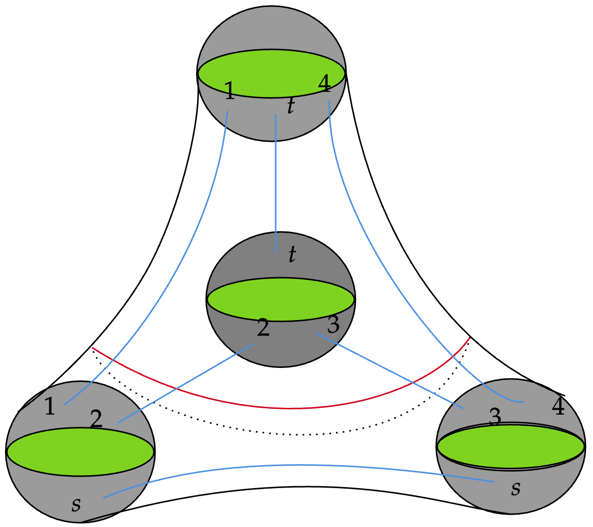
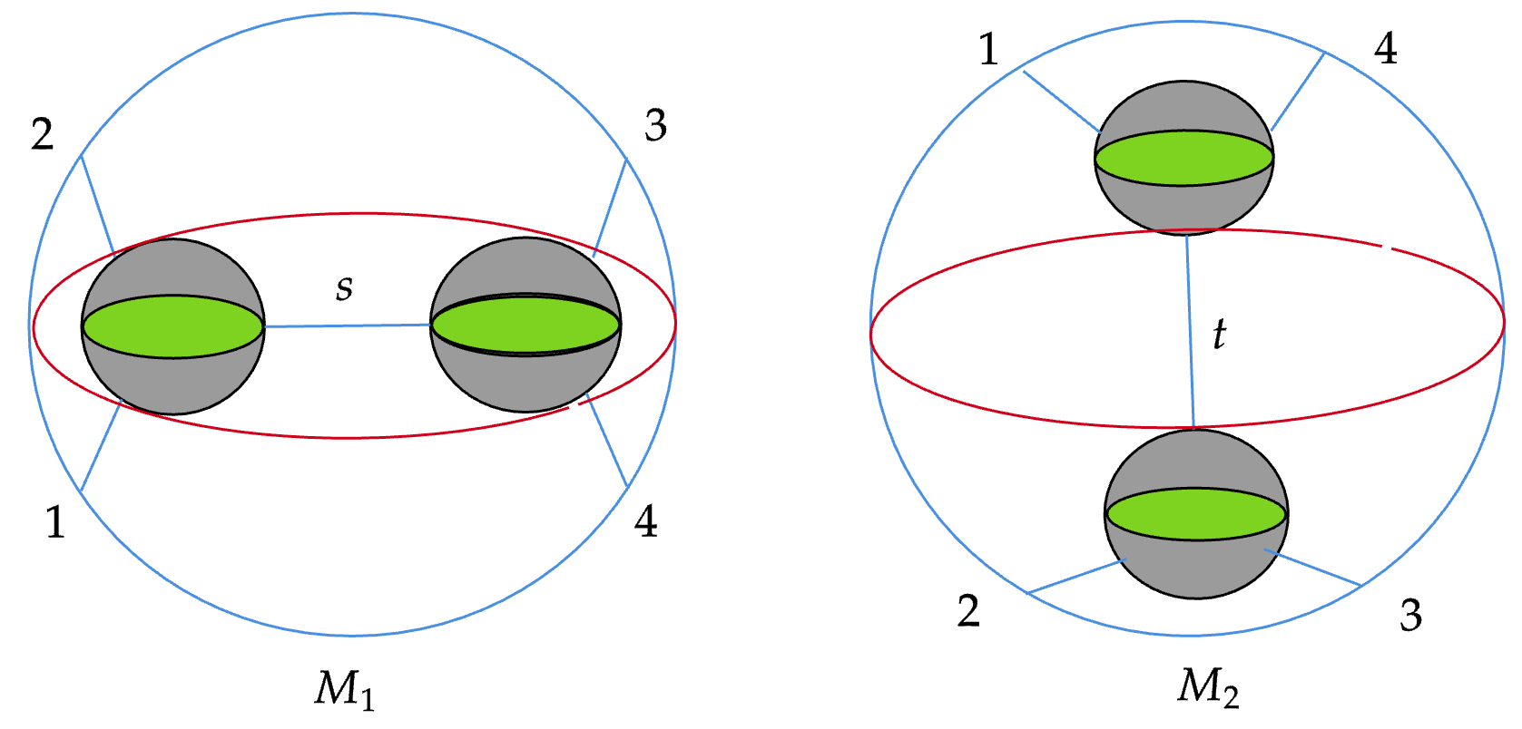
Figure 1: Figure depicting the four three punctured sphere wormholes in super-Liouville theory with non-spinning Liouvile momenta. The figure on the right side shows the Heegard splitting.

Four boundary genus zero wormhole

For a four-boundary wormhole, to find the gravitational partition function after Heegard splitting into the basis of compression bodies ($M_{1}\mbox{and }M_{2}$ in Fig. (1)), we need to use the super Virasoro fusion kernel to convert the $s$ channel block to $t$ channel block. We use the three-point super-block for the three punctured spheres, which is similar to the DOZZ structure constant in Liouville theory apart from a little modification He:2017lrg . The four-boundary super-Virasoro sphere wormhole partition function can be written as,

$$\begin{split}{Z}_{\text{SuperVir}}^{\text{Wormhole}}\Bigg{(}\begin{minipage}[h]{73.7146pt} \vspace{4pt} \scalebox{1.3}{\includegraphics[width=433.62pt]{wormhole_3.png}} \end{minipage}\hskip 19.91684pt\Bigg{)}=\frac{\mathbb{F}_{P_{\{s\}},P_{\{t\}}}\begin{bmatrix}P_{1}&P_{4}\\ P_{2}&P_{3}\end{bmatrix}}{\Omega_{0\,\,s}(P_{t})C_{NS}(P_{1},P_{4},P_{t})C_{NS}{(P_{2},P_{3},P_{t})}}\,.\end{split}$$ (51)

In evaluating the above, we used the Ponsot-Teschner fusion kernel Ponsot:1999uf , which expands $t$-channel block $\{t\}$ in terms of the complete basis of $s$-channel block $\{s\}$.The SLFT fusion kernel is given in Appendix (C). The main advantage of using such a formula is even without knowing the $\{s\}$ or $\{t\}$ channel conformal blocks, we can use the closed form of the fusion kernel to obtain the OPE density, which is one of the important ingredients to calculate/check quantities, e.g. partition function, ETH Srednicki:1995pt ; PhysRevA.43.2046 ; Rigol2007ThermalizationAI .

Partition function of a torus

Usually, the partition function for torus is written in the following way as the sum of the vacuum and non-vacuum characters Benjamin:2019stq .

$$\begin{split}{Z}_{\text{Vir}}^{\text{Torus}}\Bigg{(}\begin{minipage}[h]{73.7146pt} \vspace{4pt} \scalebox{0.8}{\includegraphics[width=433.62pt]{torus.png}} \end{minipage}\Bigg{)}=\chi_{0}(q)\chi_{0}(\bar{q})+\sum_{h,\bar{h}\geq t_{gap}}n_{h,\bar{h}}\chi_{h}(q)\bar{\chi}_{\bar{h}},\end{split}$$ (52)

where,

$$\chi_{0}(q)=(1-q)\frac{q^{-\frac{c-1}{24}}}{\eta(q)},\hskip 56.9055pt\chi_{h>0}(q)=\frac{q^{h-\frac{c-1}{24}}}{\eta(q)}$$ (53)

As we are interested in 2d CFTs with finite twist gap $2t_{gap}>0$ implying that there is no conserved current in the theory. Below we mention the modular $S$ transformation properties of the vacuum Virasoro characters and non-degenerate primaries.

The non-degenerate and the degenerate primary characters transforms as Benjamin:2019stq ,

$$\chi_{P}\Big{(}-\frac{1}{\tau}\Big{)}=\int_{0}^{\infty}dP^{\prime}S_{P}^{p^{\prime}}\chi_{p^{\prime}},\,\,\,\chi_{m,n}\Big{(}-\frac{1}{\tau}\Big{)}=\int_{0}^{\infty}dp^{\prime}S_{m,n}^{P^{\prime}}\chi_{P^{\prime}}.$$ (54)

with $S_{m,n}^{P^{\prime}}=2\sqrt{2}\sinh(\pi mP^{\prime}b^{-1})\sinh(\pi nP^{\prime}b)$ and $S_{P}^{P^{\prime}}=\sqrt{2}\cos(\pi PP^{\prime})$. Considering analytic continuation of the Liouville OPE for $\alpha\not{\in}[0,Q]$, we can obtain the following representation of fusion,

$$\mathbfcal{V}_{\alpha_{A}}\times\mathbfcal{V}_{\alpha_{B}}:=\sum_{\begin{subarray}{c}\alpha_{n,m}<Q/2\\ n,m\in\mathbb{Z}_{\geq 0}\end{subarray}}\mathcal{V}_{\alpha_{n,m}}+\int_{Q/2+0}^{Q/2+i\infty}d\alpha\mathcal{V}_{\alpha},$$ (55)

where $\mathbfcal{V}_{\alpha}$ is a primary with associated conformal dimension $\Delta=\alpha(Q-\alpha)\,.$ In calculating OTOC we consider $\alpha>Q/2$, so we only have the contribution from the integral.

Having all these ingredients in hand, we proceed to calculate the partition function for different topologies.

Calculation of Torus Wormhole:

After calculating the partition function of multiboundary sphere wormholes, we now proceed to calculate the partition function of the two boundary wormholes on the super-torus. The computation of the partition function is similar to the Liouville case, and the modular sum is the same as the usual (non-supersymmetric) Liouville theory. The main reason behind this is that for the even spin structure, superspace generalisation of the torus does not contain the $\textrm{Im}(\tau)$ factor or any other extra modular parameter to change the modular sum. The modular sum changes substantially when we consider the odd-spin structure on the super-torus.

Even spin structure: The two boundary torus wormhole partition function is given by,

$$\begin{split}&{Z}_{\text{Super-Vir}}^{\text{Torus-Wormhole}}\bigg{(}\begin{minipage}[h]{73.7146pt} \vspace{4pt} \scalebox{1.3}{\includegraphics[width=433.62pt]{Torus_wormhole.png}} \end{minipage}\hskip 19.91684pt\bigg{)}\\ &=\frac{1}{\sqrt{-i(\tau-\bar{\tau})}|\eta(\tau)|^{2}}\times\Bigg{(}\Bigg{|}\frac{\Theta_{3}(z=0|\tau)}{\eta(\tau)}\Bigg{|}+\Bigg{|}\frac{\Theta_{4}(z=0|\tau)}{\eta(\tau)}\Bigg{|}+\Bigg{|}\frac{\Theta_{2}(z=0|\tau)}{\eta(\tau)}\Bigg{|}\Bigg{)}\,.\end{split}$$ (56)

The $\Theta$ functions appearing in are (56) chosen according to the boundary conditions mentioned in Table (1). Now replacing $\tau\rightarrow\tau_{1}$ and $-\bar{\tau}\rightarrow\gamma\cdot\tau_{2}$, where the usual modular transformation $\gamma\cdot\tau=\frac{a\tau+b}{c\tau+d}$, with $ad-bc\neq 0$, the gravity partition function is written as,
gray!8 black

$$\tikzmarkin[disableroundedcorners=true]{ewr}(0.3,-0.5)(-0.1,0.8)Z_{\textrm{super-grav}}(T^{2}\times[0,1])=Z^{\textrm{torus-wormhole}}_{\textrm{SuperVir}}(\tau_{1})Z^{\textrm{torus-wormhole}}_{\textrm{{superVir}}}(\tau_{2})\sum_{\gamma}\frac{\sqrt{\textrm{Im}(\tau_{1})\,\textrm{Im}(\gamma\cdot\tau_{2})}}{|\tau_{1}+\gamma\cdot\tau_{2}|}\,.\tikzmarkend{ewr}$$ (57)

However, it should be noted that there exists an issue with the calculated partition function in $\mathcal{N}=1$ super-Liouville theory with the modular sum, which is similar to Eberhardt:2023mrq . For the gravitino field, there is at least one cycle around which the gravitino changes sign due to the boundary condition and in such cases, there are no zero modes.

Odd torus-Wormhole partition function: For the odd spin structure, we identify the points,

$$\begin{split}(z,\theta)\sim(z+1,\theta);\hskip 56.9055pt(z,\theta)\sim(z+\tau+\theta\delta,\theta+\delta)\,.\end{split}$$ (58)

Clearly, due to this, a function (for odd spin structure) $\xi(z,\theta)$ satisfies

$$\begin{split}&\xi(z,\theta)=\xi(z+\tau+\theta\delta,\theta+\delta)\,,\\ &\xi(z,\theta)=\xi(z+1,\theta)\,.\end{split}$$ (59)

Physically, the odd($\delta$) and the even ($\tau$) are the modular periods of $(\theta,z)$ correspond to zero modes for gravitino and the graviton (these constant modes cannot be gauged). These type of functions in (59) are also known as ‘Superelliptic’ functions. To obtain the partition function, we have the following action as Myung:1989bg ,

$$\begin{split}A^{\prime}=\frac{g}{2\pi}\int_{\mathcal{T}}d^{2}\omega&\Bigg{[}\partial_{\omega}\Phi_{1}\partial_{\bar{\omega}}\Phi_{1}+\bar{\psi}_{1}\partial_{\omega}\bar{\psi}_{1}-\psi_{1}\partial_{\bar{\omega}}\psi_{1}+\frac{\delta\bar{\delta}}{2\tau_{I}^{2}}\bar{\psi}_{1}\psi_{1}-F_{1}^{2}-\frac{i\delta}{\tau_{I}}\psi_{1}\partial_{\omega}\Phi_{1}-\frac{i\bar{\delta}}{\tau_{I}}\bar{\psi}_{1}\partial_{\bar{\omega}}\Phi_{1}\\ &+g\frac{\delta\bar{\delta}}{4\pi\tau_{I}}\bar{\psi}_{0}\psi_{0}-\frac{g\tau_{I}F_{0}^{2}}{2\pi}\Bigg{]}\,.\end{split}$$ (60)

Here the new coordinates $W=(\omega,\phi)$ is related with $Z=(z,\theta)$ in the following way,

$$z=\omega+\phi\delta\frac{\omega_{I}}{\tau_{I}},\,\,\,\,\,\,\theta=\phi+\delta\frac{\omega_{I}}{\tau_{I}}\,.$$ (61)

$\omega_{I}$ and $\tau_{I}$ denotes the imaginary part of $\omega,\tau$. The action (60) comes from the expansion of

$$A^{\prime}=\frac{g}{2\pi}\int_{s\mathcal{T}}d^{4}zD_{\theta}JD_{\bar{\theta}}J$$ (62)

with

$$J(W,\bar{W})=\Phi(\omega,\bar{\omega})+\phi\psi(\omega,\bar{\omega})-\bar{\phi}\bar{\psi}(\omega,\bar{\omega})+\bar{\phi}\phi F(\omega,\bar{\omega})\,.$$ (63)

The auxiliary field F can be removed by using the equation of motion. The total partition function is given by Myung:1989bg ,

$$\begin{split}Z={\int D\Phi_{1}e^{-A_{\Phi_{1}}}}\leavevmode\nobreak\ {\int DS_{0}\,D[\psi_{1},\bar{\psi}_{1}]e^{-A_{r}}}=Z_{0}\cdot Z_{1},\end{split}$$ (64)

where,

$$\begin{split}&Z_{0}=\Bigg{(}\frac{g}{2\tau_{I}}\Bigg{)}^{1/2}\frac{1}{|\eta(\tau)|^{2}}\,\,,\quad Z_{1}=\frac{\bar{\delta}\delta}{\tau_{I}}|\eta(\tau)|^{2},\end{split}$$ (65)

where, $DS_{0}=CdF_{0}d\psi_{0}d\bar{\psi_{0}}$ and $A_{r}=A^{\prime}-A_{\Phi_{1}}$. $Z_{0}$ comes from the contribution of zero modes of action, and $Z_{1}$ comes from the path integral over $\Phi_{1}$. In odd super-torus, the modular transformation works as,

$$\tau^{\prime}=\frac{a\tau+b}{c\tau+d},\,\,\,\,\,\,\,\,\,\,\,\,\delta^{\prime}=\frac{\delta}{(c\tau+d)^{3/2}},$$ (66)

where $\tau,\delta$ belongs to the super-torus and $\begin{bmatrix}a&b\\ c&d\end{bmatrix}\in SL(2,\mathbb{Z})\,.$ The modular sum (which gives the gravitational partition function) can be casted as,

$$Z^{\textrm{odd}}_{\textrm{Supergrav}}(T^{2}\times[0,1])=\sum_{\begin{subarray}{c}\gamma\in\frac{a\tau+b}{c\tau+d}\\ \gamma^{\prime}\in\frac{\delta}{(c\tau+d)^{3/2}}\end{subarray}}\left|\frac{(\gamma^{\prime}\cdot\delta_{2})\,\delta_{1}}{(\tau_{1}+\gamma\cdot\tau_{2})^{3/2}}\right|^{2}$$ (67)

We will leave performing the modular sum and its extensions for future work. For this case, the boundary conditions are periodic in both cycles of the torus. Hence the gravitino field does not change its sign, and therefore, there are zero modes appearing in theory. Due to this, the laplacian operator does not yield an inverse. This is one of the important subtleties involved in the "PP" boundary condition. So, we perform the calculation where the fermionic mode is at least antiperiodic in one of the cycles of the torus (i.e. for an even spin structure), leaving the complete analysis for the odd spin case for future studies.

In this section we focused on the computation of partition function. Now, a natural question arises: What are the gravitational descriptions of higher point functions? The answer to this question is a bit tricky. The direct answer is that, although there is a general holographic correspondence between 3D gravity and 2D CFT working for ensemble averages of large charge CFTs, they reproduce the gravitational counterparts in very few cases. For the Gaussian ensemble, it reproduces the gravitational result upto two boundary wormholes deBoer:2024kat . However, for wormholes with more than two boundaries, non-gaussianities Belin:2023efa are important, and Gaussian contractions lead to wrong results. Partial progress has been made by considering non-gaussian contractions to reproduce the gravitational counterparts in deBoer:2024kat . In VTQFT formalism, one can define states in super-Virasoro CFT as four punctured torus surfaces, and one can calculate the gravitational counterpart by squaring and performing the modular sum. Generally, the one-punctured torus wormholes correspond to carving out a solid tori from the interior and glueing along the inner torus boundary. These types of wormholes are called Maldacena-Maoz wormholes Maldacena:2004rf . Furthermore, one can think of the higher point functions as conical defects propagating in the bulk of such a wormhole.

In our paper, we focus on calculating the fount-point OTOC on torus (leading geometry), taking resort of (super-) VTQFT braiding transformations. One can calculate the contribution to the OTOC in the bulk silde coming from the torus-wormhole, by taking the inner-product of four-point conformal blocks on torus. In the next section we present the details of the computation of OTOC.

4 Four-point Conformal blocks on $T^{2}$

In this section, we proceed to evaluate the torus ($T^{2}$) four-point block in the large-charge ($c\rightarrow\infty$) regime. One way to evaluate this is to use the monodromy method for super-torus using super-Ward identities. However, we use the procedure mentioned in Alkalaev:2017bzx to calculate the large charge conformal blocks using the recursive approach. The calculated conformal blocks are Necklace channel conformal blocks. We showcase the formalism to calculate the OPE channel blocks from the necklace channel blocks using some basic fusion and modular transformations. To begin with, we first review what is the torus one-point function in this approach in Liouville CFT.

NS Vertex operators

Super-descendants $\Phi_{\Delta,\bar{\Delta}}(\xi,\bar{\xi}|Z,\bar{Z})$ of the super-primary field $\Phi_{\Delta,\bar{\Delta}}(Z,\bar{Z})=\Phi_{\Delta,\bar{\Delta}}(\nu,\bar{\nu}|Z,\bar{Z})$ are given by the following relation,

$$\begin{split}&\Phi_{\Delta,\bar{\Delta}}(L_{-m}\xi,\bar{\xi}|Z,\bar{Z})=\oint\frac{dW}{2\pi i}(W-Z)^{1-m}T(W)\Phi_{\Delta,\bar{\Delta}}(\xi,\bar{\xi}|Z,\bar{Z})\,\,\,\,\,\,\,\,\,\,\,\,\,\,\,m\in\mathbb{N}\,,\\ &\Phi_{\Delta,\bar{\Delta}}(G_{-k}\xi,\bar{\xi}|Z,\bar{Z})=\oint\frac{dW}{2\pi i}(W-Z)^{1/2-k}T(W)\Phi_{\Delta,\bar{\Delta}}(\xi,\bar{\xi}|Z,\bar{Z})\,\,\,\,\,\,\,\,\,\,\,\,\,\,\,k\in\mathbb{N}-1/2\,.\end{split}$$ (68)

Few conformal ward identities can be found in Suchanek:2010kq ; Hadasz:2006qb .

Liouville Torus one-point function:

The torus one-point function $\phi_{\lambda,\bar{\lambda}}$ with the modular parameter $\tau$ can be casted as Suchanek:2010kq ,

$$\begin{split}\langle\phi_{\lambda,\bar{\lambda}}\rangle&=(q\bar{q})^{-c/24}\sum_{\Delta,\bar{\Delta}}\,\,\sum_{f,\bar{f}\in\frac{1}{2}\bigcup\{0\}}q^{\Delta+f}\bar{q}^{\bar{\Delta}+\bar{f}}\sum_{\begin{subarray}{c}f=|M|+|K|=|N|+|L|\\ \scriptstyle{\bar{f}=|\bar{M}|+|\bar{K}|=|\bar{N}|+|\bar{L}|}\end{subarray}}[B^{f}_{\Delta}]^{MK,NL}[B^{\bar{f}}_{\bar{\Delta}}]^{\bar{M}\bar{K},\bar{N}\bar{L}}\\ &\times\langle\langle\Delta|_{MK}\bigotimes\langle\bar{\Delta}|_{\bar{M}\bar{K}}|\phi_{\lambda,\bar{\lambda}}(1,1)||\Delta\rangle_{NL}\bigotimes|\bar{\Delta}\rangle_{\bar{N}\bar{L}}\rangle\end{split}$$ (69)

where $q=\exp(2\pi i\tau)$ and the sum runs over the whole supermodule of the Neveu-schwarz(NS) sector. The matrices $[B^{f}_{\Delta}]^{MK,NL}$, $[B^{f}_{\bar{\Delta}}]^{\bar{M}\bar{K},\bar{N}\bar{L}}$ are the inverse of the Gram matrices, and they are given by,

$$[B^{f}_{\Delta}]_{MK,NL}=\langle\langle\Delta|_{MK}\Big{|}|\Delta\rangle_{NL}\rangle,\leavevmode\nobreak\ \leavevmode\nobreak\ \leavevmode\nobreak\ \leavevmode\nobreak\ \leavevmode\nobreak\ \leavevmode\nobreak\ \leavevmode\nobreak\ \leavevmode\nobreak\ \leavevmode\nobreak\ [B^{\bar{f}}_{\bar{\Delta}}]_{\bar{M}\bar{K},\bar{N}\bar{L}}=\langle\langle\bar{\Delta}|_{\bar{M}\bar{K}}\Big{|}|\bar{\Delta}\rangle_{\bar{N}\bar{L}}\rangle$$

calculated in the standard NS sector. Apart from this, we have,

$$|\Delta\rangle_{MK}=L_{-M}G_{-K}|\Delta\rangle=L_{-m_{j}}\cdots L_{-m_{1}}G_{-k_{i}}\cdots G_{-k_{1}}|\Delta\rangle$$

where $k_{i}>\cdots>k_{1}$ and $k_{s}\in\mathbb{N}-1/2$ alongwith $m_{j}\geq\cdots\geq m_{1},m_{r}\in\mathbb{N}.$ For $K,L\mbox{ and }\bar{K},\bar{L}$ having the same parity one has,

$$\begin{split}\langle\langle\Delta|_{MK}\bigotimes{\langle\bar{\Delta}|_{\bar{M}\bar{K}}}\Big{|}\phi_{\lambda,\bar{\lambda}}(1,1)\Big{|}|\Delta\rangle_{NL}\bigotimes|\bar{\Delta}\rangle_{\bar{N}\bar{L}}\rangle=\rho_{NN}(\Delta_{MK},\Delta_{\lambda},\Delta_{NL})\rho_{NN}({\bar{\Delta}_{\bar{M}\bar{K}}},\bar{\Delta}_{\bar{\lambda}},{\bar{\Delta}_{\bar{N}\bar{L}}})C^{\lambda,\bar{\lambda}}_{\Delta,\bar{\Delta}},\end{split}$$ (70)

where the quantity $C^{\lambda,\bar{\lambda}}_{\Delta,\bar{\Delta}}$ is the primary three-point structure constants. The quantity $\rho$ can be computed by taking the product of fusion polynomials.

In the next subsection, we move on to the computation of the torus four-point conformal block, which is relevant for computing the OTOC Kusuki:2019gjs ; Roberts:2014ifa .

Super Liouville four-point function on torus:

Now, we proceed to compute the torus four-point block in $s$-channel. The $t$-channel block can be computed by using the fusion kernel method or by taking the OPE directly in the different channels. Then, we will show how to achieve the global blocks in the $c\rightarrow\infty$ limit. Recalling that $\langle\tilde{\Delta}_{m}|\phi_{k}(z_{k})|\tilde{\Delta}_{l}\rangle=C_{\tilde{\Delta}_{m}\Delta_{k}\tilde{\Delta}_{l}}z_{k}^{\tilde{\Delta}_{m}-\Delta_{k}-\tilde{\Delta}_{l}}$ are the structure constants, we write the four point function for super-Liouville theory as,

$$\begin{split}&\langle\Phi_{1}(Z_{1},\bar{Z}_{1})\Phi_{2}(Z_{2},\bar{Z}_{2})\Phi_{3}(Z_{3},\bar{Z}_{3})\Phi_{4}(Z_{4},\bar{Z}_{4})\rangle_{\tau}\\ &=\sum_{\tilde{\Delta}_{1},\tilde{\Delta}_{2},\tilde{\Delta}_{3},\tilde{\Delta}_{4}}C_{\tilde{\Delta}_{1}\Delta_{1}\tilde{\Delta}_{2}}C_{\tilde{\Delta}_{2}\Delta_{2}\tilde{\Delta}_{3}}C_{\tilde{\Delta}_{3}\Delta_{3}\tilde{\Delta}_{4}}C_{\tilde{\Delta}_{4}\Delta_{4}\tilde{\Delta}_{1}}\\ &\times Z_{1}^{\tilde{\Delta}_{1}-\Delta_{1}-\tilde{\Delta}_{2}}Z_{2}^{\tilde{\Delta}_{2}-\Delta_{2}-\tilde{\Delta}_{3}}Z_{3}^{\tilde{\Delta}_{3}-\Delta_{3}-\tilde{\Delta}_{4}}Z_{4}^{\tilde{\Delta}_{4}-\Delta_{4}-\tilde{\Delta}_{1}}\Big{[}\mathcal{F}_{c}^{\{s\}\Delta_{1,2,3,4}\tilde{\Delta}_{1,2,3,4}}(q,Z_{1,2,3,4})\Big{]}\times(\textrm{anti-holomorphic})\end{split}$$ (71)

where the necklace-channel conformal block is denoted by $\mathcal{F}^{\{s\}}$ and the expression is given by,

$$\begin{split}\mathcal{F}^{\{s\}}_{c}&=q^{c/24-\tilde{\Delta}_{1}}\sum_{n,m,r,g=0}^{\infty}q^{n}\sum_{\begin{subarray}{c}|M|+|K|=|N|+|L|=n\\ |S|+|J|=|T|+|P|=m\\ |O|+|Y|=|U|+|V|=r\\ |E|+|W|=|C|+|X|=g\end{subarray}}[B^{1}_{\Delta}]^{MK,NL}\frac{\langle\tilde{\Delta}_{1},MK|\Phi_{1}(Z_{1})|SJ,\tilde{\Delta}_{2}\rangle}{\langle\tilde{\Delta}_{1}|\Phi_{1}(Z_{1})|\tilde{\Delta}_{2}\rangle}[B^{2}_{\Delta}]^{SJ,TP}\\ &\times\frac{\langle\tilde{\Delta}_{2},TP|\Phi_{2}(Z_{2})|OY,\tilde{\Delta}_{3}\rangle}{\langle\tilde{\Delta}_{2}|\Phi_{2}(Z_{2})|\tilde{\Delta}_{3}\rangle}[B^{3}_{\Delta}]^{OY,UV}\frac{\langle\tilde{\Delta}_{3},UV|\Phi_{3}(Z_{3})|EW,\tilde{\Delta}_{4}\rangle}{\langle\tilde{\Delta}_{3}|\Phi_{3}(Z_{3})|\tilde{\Delta}_{4}\rangle}\,\,[B^{4}_{\Delta}]^{EW,CX}\frac{\langle\tilde{\Delta}_{4},CX|\Phi_{4}(Z_{4})|NL,\tilde{\Delta}_{1}\rangle}{\langle\tilde{\Delta}_{4}|\Phi_{4}(Z_{4})|\tilde{\Delta}_{1}\rangle}\,.\end{split}$$ (72)

We will be mainly focusing on the calculation of the Out-of-time-order (OTO) four-point function, which has a form of $\langle\mathcal{O}_{A}\mathcal{O}_{B}\mathcal{O}_{A}\mathcal{O}_{B}\rangle\,.$ We will set the conformal dimensions of the two primaries (super-Virasoro) inserted on the time circle in the torus to be equal while calculating the time-ordered (TO) super-Liouville four-point function. We can write the conformal block structure in the TO four-point function on the torus as, (defining $x=z_{2}/z_{1}$)

$$\begin{split}&\mathcal{F}^{\{s\}}_{\langle\Phi_{1}(z_{1},\bar{z}_{1})\Phi_{1}(z_{2},\bar{z}_{2})\Phi_{3}(z_{3},\bar{z}_{3})\Phi_{3}(z_{4},\bar{z}_{4})\rangle_{\tau}}={\bf\mathcal{A}}_{c}^{\Delta_{1,2},\tilde{\Delta}_{1,2,3,4}}(z_{1,2,3,4})+q^{1/2}{\bf\mathcal{B}}_{c}^{\Delta_{1,2,3,4},\tilde{\Delta}_{1,2,3,4}}(z_{1,2,3,4})+\mathcal{O}(q)+\cdots\,.\end{split}$$ (73)

Here $\mathcal{A}_{c}$ and $\mathcal{B}_{c}$ are given in (116) and (117) respectively. In the next section, we use the four-point function given in (71) to compute the OTOC using suitable transformation and analyze its early-time behaviour.

5 A brief tour to OTOC

The out-of-time-order correlator (OTOC) is a probe for early-time chaos. The OTOC is defined as the inner product between two states $A(t)B|0\rangle_{\beta}$ and $BA(t)|0\rangle_{\beta}$ where the operators $A$ and $B$ are separated in space by $x$ and in Lorentzian time by $t$ at the inverse temperature $\beta\,.$ The definition of the normalised OTOC is given by ,

$$\mathbfcal{C}_{\beta}(x,t):=\frac{\langle B^{\dagger}A^{\dagger}(t)B\,A(t)\rangle_{\beta}}{\sqrt{\langle B^{\dagger}A^{\dagger}(t)B(t)\,A\rangle_{\beta}\langle A^{\dagger}(t)B^{\dagger}B\,A(t)\rangle_{\beta}}}\,.$$ (74)

To compute the OTOC, we do the analytic continuation of the following TO correlator,
$\langle B^{\dagger}(z_{1},\bar{z}_{1})B(z_{2},\bar{z}_{2})A^{\dagger}(z_{3},\bar{z}_{3})A(z_{4},\bar{z}_{4})\rangle_{\beta}$, so that the operator ordering becomes $\langle B^{\dagger}A^{\dagger}(t)B\,A(t)\rangle_{\beta}\,.$

This can be obtained by the following choice of coordinates on the thermal cylinder as Roberts:2014ifa ,

$$\begin{split}&z_{1}=e^{\frac{2\pi}{\beta}(t+i\epsilon_{1})},\hskip 56.9055pt\bar{z}_{1}=e^{-\frac{2\pi}{\beta}(t+i\epsilon_{1})}\,,\\ &z_{2}=e^{\frac{2\pi}{\beta}(t+i\epsilon_{2})},\hskip 56.9055pt\bar{z}_{2}=e^{-\frac{2\pi}{\beta}(t+i\epsilon_{1})}\,,\\ &z_{3}=e^{\frac{2\pi}{\beta}(x+i\epsilon_{3})},\hskip 56.9055pt\bar{z}_{3}=e^{-\frac{2\pi}{\beta}(x-i\epsilon_{3})}\,,\\ &z_{4}=e^{\frac{2\pi}{\beta}(x+i\epsilon_{4})},\hskip 56.9055pt\bar{z}_{4}=e^{\frac{2\pi}{\beta}(x-i\epsilon_{4})}\\ &\end{split}$$ (75)

where we analytically continued the correlator to the real-time considering $\epsilon_{1}<\epsilon_{3}<\epsilon_{2}<\epsilon_{4}$.

At late times, the OTOC is exponentially damped for truly chaotic systems, and it may decay polynomically for non-chaotic models. The time evolution of the cross-ratio $z$ is given by $(1-z)\rightarrow(1-z)e^{-2\pi i}$, which means, in turn, that the late time behaviour of the OTOC is given by the corresponding Regge limit of the correlator.

In this case, the cross-ratio on the complex plane is given by,

$$z\approx e^{\frac{-2\pi}{\beta}(x-t)}\epsilon_{12}^{*}\epsilon_{34}\,,\hskip 56.9055pt\bar{z}\approx-e^{\frac{-2\pi}{\beta}(x+t)}\epsilon_{12}^{*}\epsilon_{34}$$ (76)

Where we use the abbreviation,

$$\epsilon_{ij}=i\Big{(}e^{\frac{2\pi}{\beta}i\epsilon_{i}}-e^{\frac{2\pi}{\beta}i\epsilon_{j}}\Big{)}$$ (77)

Now, One needs to pick the monodromy around the branch cut in $z\sim[1,\infty)$.

We shall use the below limits of fusion kernel in case of finding the OTOC.

$$\begin{split}\mathbb{F}_{P_{3},P_{t}}\begin{bmatrix}P_{3}&P_{2}\\ \mathbb{1}&P_{1}\end{bmatrix}&=\delta(P_{1}-P_{t})\ ,\\ \mathbb{F}_{\mathbb{1},P_{t}}\begin{bmatrix}P_{3}&P_{2}\\ P_{3}&P_{2}\end{bmatrix}&=C_{NS}(P_{2},P_{3},P_{t})\,\frac{W_{NS}(\alpha_{t})}{W_{NS}(Q-\alpha_{t})}\ ,\\ \mathbb{S}_{\mathbb{1},P}[\mathbb{1}]&=W_{NS}(\alpha)W_{NS}(Q-\alpha)\ .\end{split}$$ (78)

In case of finding the OTOC on the torus one needs to remember that there are two cycles in this specific topology. One is called the spatial circle, and the other one is called the time circle. We are interested in finding this probe of chaos (OTOC) for super-Liouville matter insertions. For calculating the Out-of-time-order correlator in this case, we need to perform an R-transformation on the time-ordered four-point function. Pictorially this can be described as Mertens:2022irh ,

$$\begin{split}\begin{minipage}[h]{73.7146pt} \vspace{4pt} \scalebox{0.85}{\includegraphics[width=433.62pt]{OTO.png}} \end{minipage}\hskip 8.5359pt=\int d\alpha_{s}\mathbb{R}^{(s)\gamma,\epsilon}_{\alpha_{s}\alpha_{t}}\begin{bmatrix}\alpha_{B}&\alpha_{A}\\ \alpha_{\psi}&\alpha_{\psi^{\prime}}\end{bmatrix}\begin{minipage}[h]{73.7146pt} \vspace{4pt} \scalebox{0.85}{\includegraphics[width=433.62pt]{TO.png}} \end{minipage}\end{split}$$ (79)

In the above equation, $\mathbb{R}$ matrix is related to the fusion matrix in the following fashion for Virasoro respresentation as Suchanek:2010kq ,

$$\mathbb{R}_{\alpha_{s}\alpha_{t}}\begin{bmatrix}\alpha_{3}&\alpha_{2}\\ \alpha_{4}&\alpha_{1}\end{bmatrix}=e^{2\pi i(\Delta_{2}+\Delta_{4}-\Delta_{s}-\Delta_{t})}\mathbb{F}_{\alpha_{s}\alpha_{t}}\begin{bmatrix}\alpha_{3}&\alpha_{2}\\ \alpha_{4}&\alpha_{1}\end{bmatrix}\,.$$ (80)

The $\mathbb{F}$-matrix can be written in terms of quantum 6j symbols via,

$$\mathbb{F}_{\alpha_{s}\alpha_{t}}\begin{bmatrix}\alpha_{3}&\alpha_{2}\\ \alpha_{4}&\alpha_{1}\end{bmatrix}=|S_{b}(2\alpha_{t})S_{b}(2\alpha_{s})|\sqrt{\frac{C(\alpha_{4},\alpha_{t},\alpha_{1})C(\bar{\alpha}_{t},\alpha_{3},\alpha_{2})}{C(\alpha_{3},\alpha_{4},\alpha_{s})C(\bar{\alpha}_{s},\alpha_{2},\alpha_{1})}}\begin{Bmatrix}\alpha_{1}&\alpha_{2}&\alpha_{s}\\ \alpha_{3}&\alpha_{4}&\alpha_{t}\end{Bmatrix}_{b}$$

where $S_{b}$ denotes the double sine function , $\alpha_{j}=\frac{Q}{2}+i\underbrace{bk_{j}}_{P_{j}}$ and $C(\alpha_{1},\alpha_{2},\alpha_{s})$ are the usual DOZZ coefficients in the Liouville theory. The 6j symbols can be found in Blommaert:2018oro . The generalization to the super-Liouville case is quite straightforward.

The necklace channel braiding $(\mathbb{R})$ matrix is given by,

$$\mathbb{R}^{\gamma,\epsilon}_{\alpha_{s}\alpha_{t}}\begin{bmatrix}\alpha_{3}&\alpha_{2}\\ \alpha_{4}&\alpha_{1}\end{bmatrix}=e^{\pi i\epsilon(\Delta_{4}+\Delta_{1}-\Delta_{s}-\Delta_{t})}\,\mathbb{R}^{\gamma}_{\alpha_{s}\alpha_{t}}\begin{bmatrix}\alpha_{3}&\alpha_{2}\\ \alpha_{4}&\alpha_{1}\end{bmatrix}\,\,\,\,\,\,\,\,\,\,\,\,\,\,\,\gamma=(e,o)\,\,\,\,\,\,\,\,\,\,\,\,\,\,\epsilon=\textrm{sign}(\textrm{Arg}\,z_{3}-\textrm{Arg}\,z_{2})$$ (81)

where,

$$\begin{split}\mathbb{R}^{\gamma}_{\alpha_{s}\alpha_{t}}\begin{bmatrix}\alpha_{3}&\alpha_{2}\\ \alpha_{4}&\alpha_{1}\end{bmatrix}=M^{\gamma}_{\alpha_{s},\alpha_{t}}\begin{bmatrix}\alpha_{3}&\alpha_{2}\\ \alpha_{4}&\alpha_{1}\end{bmatrix}\frac{\Gamma_{NS}(2\alpha_{s})\Gamma_{NS}(2Q-2\alpha_{s})}{4\Gamma_{NS}(Q-2\alpha_{t})\Gamma_{NS}(2\alpha_{t}-Q)}\int_{-i\infty}^{i\infty}\frac{d\tau}{i}J^{\gamma}_{\alpha_{s},\alpha_{t}}\end{split}$$ (82)

with,

$$\begin{split}M^{e}_{\alpha_{s},\alpha_{t}}\begin{bmatrix}\alpha_{3}&\alpha_{2}\\ \alpha_{4}&\alpha_{1}\end{bmatrix}=&\frac{4^{|\sigma|}\Gamma_{\sigma}(\alpha_{t}+\alpha_{4}-\alpha_{2})\Gamma_{\sigma}(\bar{\alpha}_{t}+\alpha_{4}-\alpha_{2})\Gamma_{\sigma}(\alpha_{t}+\bar{\alpha}_{4}-\alpha_{2})\Gamma_{\sigma}(\bar{\alpha}_{t}+\bar{\alpha}_{4}-\alpha_{2})}{4^{|\eta|}\Gamma_{\eta}(\alpha_{s}+\alpha_{4}-\alpha_{3})\Gamma_{\eta}(\bar{\alpha}_{s}+\alpha_{4}-\alpha_{3})\Gamma_{\eta}(\alpha_{s}+\bar{\alpha}_{4}-\alpha_{3})\Gamma_{\eta}(\bar{\alpha}_{s}+\bar{\alpha}_{4}-\alpha_{3})}\\ &\times\frac{\Gamma_{\sigma}(\alpha_{t}+\alpha_{1}-\alpha_{3})\Gamma_{\sigma}(\bar{\alpha}_{t}+\alpha_{1}-\alpha_{3})\Gamma_{\sigma}(\alpha_{t}+\bar{\alpha}_{1}-\alpha_{3})\Gamma_{\sigma}(\bar{\alpha}_{t}+\bar{\alpha}_{1}-\alpha_{3})}{\Gamma_{\eta}(\alpha_{s}+\alpha_{1}-\alpha_{2})\Gamma_{\eta}(\bar{\alpha}_{s}+\alpha_{1}-\alpha_{2})\Gamma_{\eta}(\alpha_{s}+\bar{\alpha}_{1}-\alpha_{2})\Gamma_{\eta}(\bar{\alpha}_{s}+\bar{\alpha}_{1}-\alpha_{2})}\end{split}$$ (83)

and for the even structure, the J($\tau$) matrix is given by Chorazkiewicz:2008es ,

$$J^{e}(\tau)=\begin{pmatrix}\begin{bmatrix}N&N&N&N\\ N&N&N&N\end{bmatrix}+\begin{bmatrix}R&R&R&R\\ R&R&R&R\end{bmatrix}&\frac{1}{i}\begin{bmatrix}N&N&N&N\\ R&R&N&N\end{bmatrix}+i\begin{bmatrix}R&R&R&R\\ N&N&R&R\end{bmatrix}\\ \frac{1}{i}\begin{bmatrix}N&N&N&N\\ N&N&R&R\end{bmatrix}+i\begin{bmatrix}R&R&R&R\\ R&R&N&N\end{bmatrix}&-\begin{bmatrix}N&N&N&N\\ R&R&R&R\end{bmatrix}-\begin{bmatrix}R&R&R&R\\ N&N&N&N\end{bmatrix}\end{pmatrix}$$

where we use the abbreviations,

$$\begin{bmatrix}N&N&N&N\\ N&N&N&N\end{bmatrix}=\frac{S_{NS}(\bar{\alpha}_{4}-\alpha_{3}+\alpha_{2}+\tau)S_{NS}(\alpha_{1}+\tau)S_{NS}(\alpha_{4}-\alpha_{3}+\alpha_{2}+\tau)S_{NS}(\bar{\alpha}_{1}+\tau)}{S_{NS}(\bar{\alpha}_{3}+\bar{\alpha}_{t}+\tau)S_{NS}(\bar{\alpha}_{3}+\alpha_{t}+\tau)S_{NS}(\alpha_{s}+\alpha_{2}+\tau)S_{NS}(\bar{\alpha}_{s}+\alpha_{2}+\tau)}$$ (84)

similarly,

$$\begin{bmatrix}N&R&N&R\\ N&N&N&N\end{bmatrix}=\frac{S_{NS}(\bar{\alpha}_{4}-\alpha_{3}+\alpha_{2}+\tau)S_{R}(\alpha_{1}+\tau)S_{NS}(\alpha_{4}-\alpha_{3}+\alpha_{2}+\tau)S_{R}(\bar{\alpha}_{1}+\tau)}{S_{NS}(\bar{\alpha}_{3}+\bar{\alpha}_{t}+\tau)S_{NS}(\bar{\alpha}_{3}+\alpha_{t}+\tau)S_{NS}(\alpha_{s}+\alpha_{2}+\tau)S_{NS}(\bar{\alpha}_{s}+\alpha_{2}+\tau)}\,.$$ (85)

Here, $\bar{\alpha}_{i}=Q-\alpha_{i}$. Again ,

$$\lim_{\alpha_{1}\rightarrow 0}\mathbb{R}^{e}_{\alpha_{s}\alpha_{t}}\begin{bmatrix}\alpha_{3}&\alpha_{2}\\ \alpha_{4}&\alpha_{1}\end{bmatrix}^{e}_{\lambda}={\bf\delta(\alpha_{s}-\alpha_{2})}\delta^{e}_{\lambda}\delta(P_{t}-P_{3})\,.$$

Before computing the exact form of the integral, we wish to extract the asymptotic behaviour of the 4-point necklace channel conformal block and see how it depends on the cross-ratio and the conformal dimension $\Delta_{s}$, which can easily be done using the shadow formalism Ferrara:1972kab ; Iliesiu:2015qra ; Alkalaev:2023evp .

Torus blocks: Shadow formalism

To calculate the OTOC in super-Liouville field theory on the torus one should compute the asymptotic behaviour of the necklace channel conformal block precisely Rosenhaus:2018zqn . This computation will mainly help to fix the nature of OTOC with time. We show that as there is a connection between comb channel conformal blocks and necklace channel conformal blocks, we can extract the $n$-point necklace channel conformal block from the $n+2$-point comb channel conformal block Rosenhaus:2018zqn .

$$\mathcal{F}_{N}^{(n)}(q,z|\Delta,\tilde{\Delta},\Delta_{\alpha})=\sum_{m=0}^{\infty}\frac{q^{m+\Delta_{\alpha}}A_{m}^{(n+2)}(z|\Delta,\tilde{\Delta},\Delta_{\alpha})}{m!(2\Delta_{\alpha})_{m}},$$ (86)

where,

$$A_{m}^{(n+2)}(z|\Delta,\tilde{\Delta},\Delta_{\alpha})=\lim_{\begin{subarray}{c}z_{0}\rightarrow 0\\ z_{n+1}\rightarrow 0\end{subarray}}\partial_{0}^{m}\partial_{n+1}^{m}\Big{(}z_{0}^{-2\Delta_{\alpha}}\mathcal{G}_{n+2}(1/z_{0},z,z_{n+1}|\Delta,\tilde{\Delta},\Delta_{\alpha})\Big{)}\,.$$ (87)

In (87), $\mathcal{G}_{n+2}$ denotes the $n+2$-point comb channel conformal block. We denote the external dimensions as $(\Delta,\Delta_{1}\cdots\Delta_{n})$ and the internal dimensions as $(\tilde{\Delta}_{0},\tilde{\Delta}_{1}\cdots\tilde{\Delta}_{n-2})$. In general, the computation of 6-point comb channel blocks yields the following compact form,

$$\mathcal{G}_{\tilde{\Delta}_{1},\tilde{\Delta}_{2},\tilde{\Delta}_{3}}^{\Delta_{1},\cdots\Delta_{6}}(z_{0},z,z_{n+1})=\mathcal{L}^{(\Delta_{1},\cdots\Delta_{4})}(z_{0},\cdots,z_{4})\,\chi_{0}^{\tilde{\Delta}_{0}}\chi_{1}^{\tilde{\Delta}_{1}}\chi_{2}^{\tilde{\Delta}_{2}}{\bf F_{K}}\begin{bmatrix}-\mathcal{S}_{1}&\tilde{\Delta}_{0}+\tilde{\Delta}_{1}-\Delta_{2}&\tilde{\Delta}_{1}+\tilde{\Delta}_{2}-\Delta_{3}&\,\,\,-\mathcal{S}_{2}\\ &\hskip 28.45274pt2\tilde{\Delta}_{0},\,2\tilde{\Delta}_{1},\,2\tilde{\Delta}_{2}\end{bmatrix}(\chi_{0},\chi_{1},\chi_{2})$$ (88)

where the leg-factor can be casted in a compact form as,

$$\mathcal{L}^{(\Delta_{1},\cdots\Delta_{4})}(z_{0},\cdots,z_{4})=\Big{(}\frac{z_{12}z_{34}}{z_{01}z_{02}z_{45}z_{35}}\Big{)}^{\Delta_{\alpha}}\prod_{i=0}^{3}\Big{(}\frac{z_{i,i+2}}{z_{i,i+1}z_{i+1,i+2}}\Big{)}^{\Delta_{i+1}}$$ (89)

and the comb function is given by,

$${\bf F_{K}}\begin{bmatrix}a_{1},&b_{1},\cdots b_{k-1},&a_{2}\\ &c_{1},\cdots,c_{k}\end{bmatrix}(x_{1},\cdots x_{k})=\sum_{n_{1},\cdots n_{k}=0}^{\infty}\frac{(a_{1})_{n_{1}}(b_{1})_{n_{1}+n_{2}}(b_{2})_{n_{2}+n_{3}}\cdots{(b_{k-1})_{n_{k-1}+n_{k}}(a_{2})_{n_{k}}}}{{(c_{1})_{n_{1}}\cdots(c_{k})_{n_{k}}}}\frac{x_{1}^{n_{1}}}{n_{1}!}\cdots\frac{x_{k}^{n_{k}}}{n_{k}!}\,.$$ (90)

In (88), we define the cross-ratios as,

$$\chi_{0}=\frac{z_{01}z_{23}}{z_{02}z_{13}};\,\,\,\,\,\,\chi_{1}=\frac{z_{12}z_{34}}{z_{13}z_{24}};\,\,\,\,\,\,\chi_{2}=\frac{z_{23}z_{45}}{z_{24}z_{35}}$$ (91)

and we also have used the short notation of $\Delta_{ij}=\Delta_{i}-\Delta_{j}$. ${\bf F_{K}}$ denotes the comb function. Its properties and few identitites are defined in Rosenhaus:2018zqn . In (88) we define,

$$\mathcal{S}_{1}=\Delta_{1}-\Delta_{\alpha}-\tilde{\Delta}_{0},\hskip 56.9055pt\mathcal{S}_{2}=\Delta_{4}-\Delta_{\alpha}-\tilde{\Delta}_{2}\,.$$ (92)

Now the quantity $A^{(6)}_{m}{(z|\Delta,\tilde{\Delta},\Delta_{\alpha})}$ which is related to the 4-point necklace channel block becomes,

$$\begin{split}A^{(6)}_{m}{(z|\Delta,\tilde{\Delta},\Delta_{\alpha})}=&\lim_{\begin{subarray}{c}z_{0}\rightarrow 0\\ z_{5}\rightarrow 0\end{subarray}}(\Delta_{1}-\Delta_{\alpha}-n_{1})_{m}(1-z_{0}){}^{-\Delta_{\alpha}+\Delta_{1}-m-n_{1}}(-\Delta_{4}-\Delta_{\alpha}+n_{3})_{m}(\chi_{1}-z_{5}){}^{-\Delta_{\alpha}-\Delta_{4}-m+n_{3}}\times\Xi({\bf\rho})\,,\\ &=(\Delta_{1}-\Delta_{\alpha}-n_{1})_{m}(-\Delta_{4}-\Delta_{\alpha}+n_{3})_{m}(\chi_{1}){}^{-\Delta_{\alpha}-\Delta_{4}-m+n_{3}}\,\Xi({\bf\rho})\,.\end{split}$$ (93)

Here, ${\bf\rho}$ denotes the other insertion points except $z_{0}$ and $z_{5}\,.$ $\Xi({\bf\rho})$ refers to the part of the correlation function independent of the cross-ratio. We need mainly the dependence on the cross ratio in leading behaviour to find the out-of-time-order correlator. We will use this in Sec. (5.2).

5.1 OTOC in plane for super-Liouville CFT

The leading behaviour of the $4$-point comb channel conformal block has the following form for our case as,

$$\mathcal{V}_{c}^{\Delta_{1,2,3,4},\tilde{\Delta}_{1,2,3,4}}\sim\chi_{1}^{\alpha_{s}(Q-\alpha_{s})}\,.$$ (94)

Now, to compute the OTOC we need to compute the following integral as given in (79),

$$\begin{split}\textrm{OTOC}&=\mathcal{F}_{r}\int_{Q/2}^{Q/2+i\infty}d\alpha_{s}e^{\pi i\epsilon(\tilde{\Delta}_{2}+\tilde{\Delta}_{4}-\Delta_{s}-\Delta_{t})}\frac{W_{NS}(Q)W_{NS}(\alpha_{s})}{\pi W_{NS}(Q-\alpha_{A})W_{NS}(Q-\alpha_{B})}\\ &\hskip 227.62204pt\times C_{NS}(\alpha_{s},\alpha_{A},\alpha_{B})\mathcal{V}_{c}^{\Delta_{1,2,3,4},\tilde{\Delta}_{1,2,3,4}}\mathbb{M}^{p}_{\alpha_{t},\alpha_{s}}\Big{[}\alpha_{A},\alpha_{B}\Big{]}\,,\\ \\ &=\underbrace{\lim_{P_{s}\rightarrow 0}\partial_{P_{s}}^{2}\Bigg{[}{\bf\Psi(\alpha_{A},\alpha_{B},Q,P_{s})\bf\bar{\Psi}(\bar{\alpha}_{A},\bar{\alpha}_{B},Q,\bar{P}_{s})}\mathbb{M}^{p}_{\alpha_{t},\alpha_{s}}\Big{[}\alpha_{A},\alpha_{B}\Big{]}\Bigg{]}}_{\bf\tilde{\Theta}(\alpha_{A},\alpha_{B},Q)}\mathcal{F}_{r}\int_{0}^{\infty}dP_{s}P_{s}^{2}\chi_{1}^{2P_{s}^{2}}\,,\\ &={\bf\tilde{\Theta}}(\alpha_{A},\alpha_{B},Q)\frac{\chi_{1}^{Q^{2}/4}}{(-\log(\chi_{1}))^{3/2}}\mathcal{F}_{r}\sim\chi_{1}^{Q^{2}/4}\Big{(}-\log(\chi_{1})\Big{)}^{-3/2}\mathcal{F}_{r},\hskip 28.45274pt\alpha_{A},\alpha_{B}>\frac{Q}{4}\,.\end{split}$$ (95)

Where $\mathbb{M}^{p}_{\alpha_{t},\alpha_{s}}\Big{[}\alpha_{A},\alpha_{B}\Big{]}$ is the monodromy matrix which is defined to be,

$$\mathcal{F}^{AA}_{BB}(h_{p}|\chi_{1})\xrightarrow{(1-\chi_{1})\to(1-\chi_{1})e^{2\pi i}}\int_{\mathbb{S}^{\prime}}d\alpha\leavevmode\nobreak\ \mathbb{M}^{p}_{\alpha_{t},\alpha_{s}}\Big{[}\alpha_{A},\alpha_{B}\Big{]}\,\mathcal{F}^{AA}_{BB}(h_{\alpha}|\chi_{1})$$ (96)

In (96) the contour $\mathbb{S}^{\prime}$ runs from $Q/2\to Q/2+i\infty$ and in fact it can be expressed in terms of fusion matrix as Kusuki:2019gjs ,

$$\mathbb{M}^{p}_{\alpha_{p},\alpha}\begin{bmatrix}\alpha_{A}&\alpha_{A}\\ \alpha_{B}&\alpha_{B}\end{bmatrix}=\int_{\mathbb{S}^{\prime}}d\beta e^{-2\pi i(h_{\beta}-h_{A}-h_{B})}F_{\alpha_{p},\beta}\begin{bmatrix}\alpha_{A}&\alpha_{B}\\ \alpha_{A}&\alpha_{B}\end{bmatrix}F_{\beta,\alpha}\begin{bmatrix}\alpha_{A}&\alpha_{A}\\ \alpha_{B}&\alpha_{B}\end{bmatrix}.$$ (97)

In (95) the function ${\bf\Psi(\alpha_{A},\alpha_{B},Q,P_{s})}$ is defined in (143) of Appendix (A). This behaviour of OTOC in the super-Liouville theory is exactly similar to the behaviour of OTOC obtained in Kusuki:2019gjs for the case of Liouville theory. To compute the integral, we used the saddle-point approach, and we have taken $C_{NS}$ approximated for two light conformal dimensions and one heavy conformal dimension. In deriving its the asymptotic form, we used the expression of $\Gamma_{b}(x)$ defined in Appendix (B). $\mathcal{F}_{r}$ is independent of $\alpha_{s}$ and it comes from the other remaining part of the conformal block.

5.2 OTOC on even torus

The two-point bosonic and fermionic super-Virasoro blocks in torus at leading order in $q$ is given by, gray!8 black

$$\begin{split}\tikzmarkin[disableroundedcorners=true]{werp}(0.5,-0.5)(-0.1,1)&{\color[rgb]{0,0,0}\mathbfcal{B}_{B}^{(1)}}=\,\frac{\Big{[}(\Delta_{s}+\tilde{\Delta}_{2}-\Delta_{2})(\tilde{\Delta}_{4}+\Delta_{s}-\Delta_{3})\Big{]}}{{2\Delta_{s}}}\chi_{1}+\mathcal{O}(q)\,,\\ &{\color[rgb]{0,0,0}\mathbfcal{B}_{F}^{(1)}}=\Big{[}\frac{(-\tilde{\Delta}_{2}-\Delta_{s}-\Delta_{2}+1/2)(-\Delta_{s}-\tilde{\Delta}_{4}-\Delta_{3}+1/2)}{2\Delta_{s}}\Big{]}\chi_{1}+\mathcal{O}(q)\,.\tikzmarkend{werp}\end{split}$$ (98)

In the following part, we focus on the "classical" torus conformal block, which is given by,

$$\mathcal{V}_{c}^{\Delta_{1,2,3,4},\tilde{\Delta}_{1,2,3,4}}(q,z_{1,2,3,4})=\exp(\frac{c}{6}f^{\epsilon_{1,2,3,4},\tilde{\epsilon}_{1,2,3,4}})\,\,\,\,\,\text{as}\,\,\,\ c\rightarrow\infty\,,$$ (99)

where the function f is the classical conformal block and,

$$\epsilon_{i}=\frac{\Delta_{i}}{k},\,\,\,\,\,\,\,\,\tilde{\epsilon}_{i}=\frac{\tilde{\Delta}_{i}}{k},\,\,\,\,\,\,\,\,\text{where}\,\,\,\,\,\,\,\,k=\frac{c}{6}.$$

Now, using (115) the $s$-channel block function is given by,

$$f^{\epsilon_{1,2,3,4},\tilde{\epsilon}_{1,2,3,4}}=(\tilde{\epsilon}_{1}-1/4)\log(q)+\sum_{n=0}^{\infty}q^{n}f_{n,B/F}^{(1)}(\epsilon,\tilde{\epsilon}|x,y),$$ (100)

where the first few expansion coefficients are,

$$\begin{split}&f^{(1)}_{B0}=\frac{1}{2\tilde{\epsilon}_{3}}\Big{[}\frac{(\tilde{\epsilon}_{1}+\tilde{\epsilon}_{2}-\epsilon_{1})(\tilde{\epsilon}_{2}+\tilde{\epsilon}_{3}-\epsilon_{2})}{2\tilde{\epsilon}_{2}}\chi_{1}\frac{(\tilde{\epsilon}_{3}+\tilde{\epsilon}_{4}-\epsilon_{3})(\tilde{\epsilon}_{4}+\tilde{\epsilon}_{1}-\epsilon_{4})}{2\tilde{\epsilon}_{4}}\Big{]}\,,\\ &f^{(1)}_{F0}=\frac{1}{2\tilde{\epsilon}_{3}}\Big{[}\frac{(-\tilde{\epsilon}_{1}-\tilde{\epsilon}_{2}-\epsilon_{1}+1/2)(-\tilde{\epsilon}_{2}-\tilde{\epsilon}_{3}-\epsilon_{2}+1/2)}{2\tilde{\epsilon}_{2}}\chi_{1}\frac{(-\tilde{\epsilon}_{3}-\tilde{\epsilon}_{4}-\epsilon_{3}+1/2)(-\tilde{\epsilon}_{4}-\tilde{\epsilon}_{1}-\epsilon_{4}+1/2)}{2\tilde{\epsilon}_{4}}\Big{]}\end{split}$$ (101)

with, $\chi_{1}:=\frac{z_{12}z_{34}}{z_{13}z_{24}}$ . Also, B/F denotes the bosonic or fermionic counterpart.

The out-of-time-order OPE channel conformal block can be obtained from the necklace channel conformal block by composition of three fusion($\mathbb{F}$) and one $\mathbb{S}$-move deBoer:2024kat .

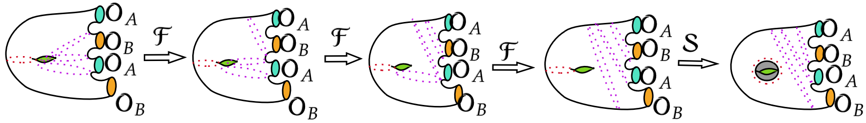
Figure 2: Figure depicting the transformation needed to get the OTO OPE block from the Necklace channel out of time order conformal block by modular-$\mathbb{S}$ transformation and the fusion-$\mathbb{F}$ transformation.

$$\begin{split}&{\color[rgb]{0,0,0}\mathcal{F}_{OPE}=\int\frac{d\tilde{\alpha}_{2}}{2}\frac{d\tilde{\alpha}_{3}}{2}\frac{d\tilde{\alpha}_{4}}{2}\frac{d\tilde{\alpha}_{1}}{2}\mathbb{F}_{\alpha_{2}^{\prime}\tilde{\alpha}_{2}}\begin{bmatrix}\alpha_{B}&\tilde{\alpha}_{3}\\ \alpha_{A}&\tilde{\alpha}_{1}\end{bmatrix}\mathbb{F}_{\alpha_{3}^{\prime}\tilde{\alpha}_{3}}\begin{bmatrix}\alpha_{A}&\tilde{\alpha}_{4}\\ \alpha_{2}^{\prime}&\tilde{\alpha}_{1}\end{bmatrix}\mathbb{F}_{\alpha_{4}^{\prime}\tilde{\alpha}_{4}}\begin{bmatrix}\alpha_{B}&\tilde{\alpha}_{1}\\ \alpha_{3}^{\prime}&\tilde{\alpha}_{1}\end{bmatrix}\mathbb{S}_{\alpha_{1}^{\prime}\tilde{\alpha}_{1}}[\alpha_{4}^{\prime}]\mathcal{F}_{N}^{OTO}}\,.\end{split}$$ (102)

Now in the limit, $\alpha_{3}^{\prime}=\alpha_{2}^{\prime}=\alpha_{B}$ and $\alpha_{A}=\epsilon\rightarrow 0$ we get,

$$\begin{split}&\mathbb{F}_{\alpha_{3}^{\prime}\tilde{\alpha}_{3}}\begin{bmatrix}\epsilon&\tilde{\alpha}_{4}\\ \alpha_{2}^{\prime}&\tilde{\alpha}_{1}\end{bmatrix}=\delta(\tilde{\alpha}_{3}-\alpha_{2}^{\prime})+\mathcal{O}(\epsilon)\,,\\ &\mathbb{F}_{\alpha_{2}^{\prime}\tilde{\alpha}_{2}}\begin{bmatrix}\alpha_{B}&\tilde{\alpha}_{3}\\ \epsilon&\tilde{\alpha}_{1}\end{bmatrix}=\delta(\tilde{\alpha}_{2}-\alpha_{B})+\mathcal{O}(\epsilon)\,.\end{split}$$ (103)

The transformations are schematically sketched in Fig. ((2)). Now considering $\alpha_{4}^{\prime},\alpha_{1}^{\prime}\rightarrow 0$, the integral simplifies to,

$$\begin{split}\mathcal{F}_{OPE}&=\int\frac{d\tilde{\alpha}_{2}}{2}\frac{d\tilde{\alpha}_{3}}{2}\frac{d\tilde{\alpha}_{4}}{2}\frac{d\tilde{\alpha}_{1}}{2}\delta(\tilde{\alpha}_{3}-\alpha_{2}^{\prime})\delta(\tilde{\alpha}_{2}-\alpha_{B})C_{{NS}}(\tilde{\alpha}_{4},\tilde{\alpha}_{1},\alpha_{B})\frac{W_{NS}(Q)W_{NS}(\tilde{\alpha}_{4})}{\pi W_{NS}(Q-\tilde{\alpha}_{1})W_{NS}(Q-\alpha_{B})}\\ &\hskip 256.0748pt\times\mathbb{S}_{\alpha_{1}^{\prime}\tilde{\alpha}_{1}}[\alpha_{4}^{\prime}]{\color[rgb]{0,0,0}\mathcal{F}_{N}^{OTO}}\,,\\ &=\int\frac{d\tilde{\alpha}_{4}}{2}\frac{d\tilde{\alpha}_{1}}{2}C_{{NS}}(\tilde{\alpha}_{4},\tilde{\alpha}_{1},\alpha_{B})\frac{W_{NS}(Q)W_{NS}(\tilde{\alpha}_{4})}{\pi W_{NS}(Q-\tilde{\alpha}_{1})W_{NS}(Q-\alpha_{B})}\mathbb{S}_{0\tilde{\alpha}_{1}}[0]\times\mathcal{F}_{N}^{OTO}|_{\tilde{\alpha}_{3}=\alpha_{2}^{\prime},\tilde{\alpha}_{2}=\alpha_{B}}+(\cdots)\end{split}$$ (104)

where in (104) we define ,

$$\begin{split}&W_{NS}(\alpha)=\frac{2(\pi\mu{\color[rgb]{0,0,0}\gamma(\frac{bQ}{2}))}^{-\frac{Q-2\alpha}{2b}}\pi(\alpha-Q/2)}{\Gamma(1+b(\alpha-Q/2))\Gamma(1+\frac{1}{b}(\alpha-Q/2))}\end{split}$$ (105)

where $\gamma(x)=\frac{\Gamma(x)}{\Gamma(1-x)}$, and the structure constant is given by,

$$\begin{split}C_{NS}(\alpha_{1},\alpha_{2},\alpha_{3})&=\lambda^{(Q-\sum_{i=1}^{3}\alpha_{i})/b}\\ &\times\frac{\Upsilon^{\prime}_{NS}(0)\Upsilon_{NS}(2\alpha_{1})\Upsilon_{NS}(2\alpha_{2})\Upsilon_{NS}(2\alpha_{3})}{\Upsilon_{NS}(\alpha_{1}+\alpha_{2}+\alpha_{3}-Q)\Upsilon_{NS}(\alpha_{1}+\alpha_{2}-\alpha_{3})\Upsilon_{NS}(-\alpha_{1}+\alpha_{2}+\alpha_{3})\Upsilon_{NS}(-\alpha_{3}+\alpha_{1}-\alpha_{2})}\end{split}$$ (106)

with $\lambda=\pi\mu\gamma(bQ/2)b^{1-b^{2}}\,.$ $\mathcal{F}^{OTO}_{N}$ is the out-of-time-order conformal block. Also we need the following modular-$\mathbb{S}$ transformation matrix elements,

$$\mathbb{S}_{0,\alpha_{1}}[0]=\textrm{sin}(\pi b^{-1}(\alpha_{1}-Q/2))\textrm{sin}(\pi b(\alpha_{1}-Q/2))\,,$$ (107)

$$\mathbb{S}_{0,\alpha_{3}}[0]=\textrm{sin}(\pi b^{-1}(\alpha_{3}-Q/2))\textrm{sin}(\pi b(\alpha_{3}-Q/2))\,.$$ (108)

Behaviour of OTOC with time:

In the case of torus, the OTOC can be found by using the out-of-time order necklace channel conformal block.

The bare n-point necklace channel torus block is given by,

$$\mathcal{V}^{h}_{\Delta}(\rho)=\,\prod_{i=1}^{n}\rho_{i}^{\tilde{\Delta}_{i}}\,\,{\bf F_{K}}\begin{bmatrix}\tilde{\Delta}_{1}+\tilde{\Delta}_{2}-\Delta_{1}&\tilde{\Delta}_{2}+\tilde{\Delta}_{3}-\Delta_{2}&\cdots&\,\,\,\tilde{\Delta}_{n}+\tilde{\Delta}_{1}-\Delta_{n}\\ &\hskip 28.45274pt2\tilde{\Delta}_{1},\,2\tilde{\Delta}_{2},\,2\tilde{\Delta}_{3},\cdots,2\Delta_{n}\end{bmatrix}(\rho_{1},\rho_{2},\cdots,\rho_{n})$$ (109)

where the cross-ratios on the torus are defined as,

$$\begin{split}&\rho_{1}=\frac{qz_{12}z_{n-1,n}}{(z_{n-1}-qz_{1})(z_{n}-qz_{2})}=-q\chi_{1},\hskip 71.13188pt\rho_{2}=\frac{z_{23}(z_{n}-qz_{1})}{z_{13}(z_{n}-qz_{2})}=1-\chi_{1}\,,\\ &\rho_{n}=\frac{z_{23}(z_{n}-qz_{1})}{z_{13}(z_{n}-qz_{2})}=\chi_{1},\hskip 128.0374pt\rho_{i}=\frac{z_{i-2,i-1}z_{i,i+1}}{z_{i-2,i}z_{i-1,i+1}}=\chi_{1}-1\,,\hskip 28.45274pt\mbox{for}\,\,\,\,3\leq i\leq n-1\,.\end{split}$$ (110)

The above cross-ratios are obtained for the configuration $z_{1}=0,z_{2}=\chi_{1},z_{3}=1,z_{4}=\infty$. The monodromy ($\mathbb{M}_{1}$) around $\chi_{1}=1$ is given by,

$$\begin{split}\mathbb{M}^{T}_{1}[\mathcal{V}^{h}_{\Delta}]=\lim_{\epsilon\rightarrow 0}&\,\pi(-1)^{\tilde{\Delta}_{4}}\chi_{1}^{\tilde{\Delta}_{3}}(-q\chi_{1})^{\tilde{\Delta}_{1}}\csc(\pi(-\tilde{\Delta}_{1}-\tilde{\Delta}_{3}+\Delta_{1}+\Delta_{2}))\Gamma(2\tilde{\Delta}_{2})\,\,\,_{2}F_{1}(-\Delta_{2}+\tilde{\Delta}_{1}+\tilde{\Delta}_{4},-\Delta_{1}+\tilde{\Delta}_{3}+\tilde{\Delta}_{4};2\tilde{\Delta}_{4};-1)\\ &\leavevmode\nobreak\ \leavevmode\nobreak\ \leavevmode\nobreak\ \leavevmode\nobreak\ \leavevmode\nobreak\ \leavevmode\nobreak\ \leavevmode\nobreak\ \leavevmode\nobreak\ \leavevmode\nobreak\ \leavevmode\nobreak\ \leavevmode\nobreak\ \leavevmode\nobreak\ \leavevmode\nobreak\ \leavevmode\nobreak\ \leavevmode\nobreak\ \leavevmode\nobreak\ \leavevmode\nobreak\ \leavevmode\nobreak\ \leavevmode\nobreak\ \leavevmode\nobreak\ \leavevmode\nobreak\ \leavevmode\nobreak\ \leavevmode\nobreak\ \Bigg{(}\frac{1}{\Gamma(\Delta_{1}-\tilde{\Delta}_{1}+\tilde{\Delta}_{2})\Gamma(\Delta_{2}+\tilde{\Delta}_{2}-\tilde{\Delta}_{3})\Gamma(-\Delta_{1}-\Delta_{2}+\tilde{\Delta}_{1}+\tilde{\Delta}_{3}+1)}\\ &\hskip 128.0374pt-\frac{e^{-\frac{1}{2}i\pi(-\tilde{\Delta}_{1}-\tilde{\Delta}_{3}+\Delta_{1}+\Delta_{2})}(2\pi)^{-\tilde{\Delta}_{1}-\tilde{\Delta}_{3}+\Delta_{1}+\Delta_{2}}\epsilon^{-\tilde{\Delta}_{1}-\tilde{\Delta}_{3}+\Delta_{1}+\Delta_{2}}}{\Gamma(-\Delta_{1}+\tilde{\Delta}_{1}+\tilde{\Delta}_{2})\Gamma(\Delta_{1}+\Delta_{2}-\tilde{\Delta}_{1}-\tilde{\Delta}_{3}+1)\Gamma(-\Delta_{2}+\tilde{\Delta}_{2}+\tilde{\Delta}_{3})}\Bigg{)}.\end{split}$$ (111)

In Fig. (3), we have shown the plot of super-Liouville OTOC for real and imaginary parts. The leading behaviour with respect to time can be easily extracted by substituting Kudler-Flam:2019kxq ,

$$\tau=i\,\frac{K_{1}(1-\chi_{1s})}{K_{1}(\chi_{1s})},\leavevmode\nobreak\ \leavevmode\nobreak\ \leavevmode\nobreak\ \leavevmode\nobreak\ \leavevmode\nobreak\ \chi_{1s}=\left(\frac{\Theta_{2s}(e^{i\pi\tau})}{\Theta_{3s}(e^{i\pi\tau})}\right)^{4}.$$ (112)

in (95). $K_{1}(z)$ are elliptic integral of the first kind. The monodromy around $\chi_{1s}=1$ is mapped to torus modular parameter via ,

$$\tau\to\frac{\tau}{1+2\tau},\leavevmode\nobreak\ \leavevmode\nobreak\ \leavevmode\nobreak\ \leavevmode\nobreak\ \bar{\tau}\to\bar{\tau}.$$ (113)

The behaviour of the holomorphic part of OTOC in time is given by,

$$\textrm{OTOC}\xrightarrow{\chi_{1}\sim 0}\frac{(-ie^{-\frac{2\pi t}{\beta}})^{\frac{Q^{2}}{4}}\Bigg{(}i\exp\Big{[}-\frac{2\pi\Big{(}t\,K_{1}(-ie^{-\frac{2\pi t}{\beta}})+(\beta+2it)\,K_{1}(1+ie^{-\frac{2\pi t}{\beta}})\Big{)}}{\beta\Big{(}K_{1}(-ie^{-\frac{2\pi t}{\beta}})+2i\,K_{1}(1+i\,e^{-\frac{2\pi t}{\beta}})\Big{)}}\Big{]}\Bigg{)}^{\tilde{\Delta}_{1}}}{\Big{(}-\log(-ie^{-\frac{2\pi t}{\beta}})\Big{)}^{3/2}}.$$ (114)

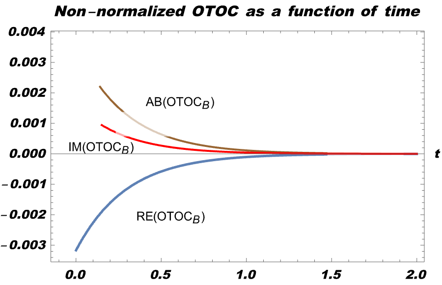
Figure 3: Figure depicting the plot of non-normalized Out-of-time-order correlator for the case of super-Liouville OTOC. The red curve depicts the real part of OTOC, and the red curve denotes the imaginary part of the OTOC. Brown curve denotes absolute value of the OTOC. The real part of the OTOC saturates at zero value at late time. Similarly the imaginary part saturates after decaying at the specific same value.

It’s evident from (non-normalized) (114) that the early-time behaviour of the OTOC does not show a simple exponential decay, i.e. it is (the real part of it) not simply of the form $\alpha-\beta e^{\lambda_{L}\,t}\,$ Fig. (3) shows the plot of the real, imaginary and absolute value of the non-normalized OTOC. This is quite distinct from what is known for the Schwarzian theory dual to JT gravity Maldacena:2016hyu . Further studies are required, including subleading corrections from the geometry, to understand its implication for quantum chaos better.

6 Conclusion and Outlook

Mainly motivated by the aspects of Topological QFT and Gravity, in this paper, we discuss how to compute the partition function of $\mathcal{N}=1$ super-Liouville theory using super-Virasoro TQFT. Due to different spin structures related to the super-torus, the bosonic or fermionic fields may or may not have zero modes. Correspondingly, the path integral and the modular sum changes. Apart from calculating partition functions for different topologies with sphere and torus boundaries, we also compute the OTOC on the torus, including the fermionic contribution to probe the early-time chaotic regime. As a probe matter, we include super-Liouville primaries in the boundary of the torus. Below, we summarize the main findings of the paper,

• First, we show that the claim of Eberhardt:2023mrq , that the gravitational partition function is equal to the sum of the modulus square of the Virasoro partition function from the Teichmuller $\times$ Teichmuller correspondence also holds for the $\mathcal{N}=1$ super-Liouville theory. We claimed and showed that the inner product of the superconformal blocks with two different Liouville momenta satisfies delta function type normalization. The bulk mapping class group (MCG) becomes a subset of the boundary mapping class group for Riemann surfaces with boundaries. Due to this, we needed to perform an extra modular sum to compute the gravitational partition function. The modular sum depends on the spin structure corresponding to the different boundary conditions.

• Second, we compute the partition function of supergravity by using the super-Virasoro TQFT. Apart from the spherical boundary, we also consider torus wormholes. Different spin structures lead to different partition functions. Odd spin structures change the boundary condition so that the zero modes contribute, and we also had to sum over odd modular parameter transformations.

• Eventually, we calculate the OTOC on the super-torus with super-Liouville matter insertions. For this purpose, we first compute the necklace channel out-of-time-order conformal block in the large charge ($c\rightarrow\infty$) limit. In this semiclassical limit, one can see that the conformal blocks are exponentiated. One should be able to verify this using the monodromy method. However, in the torus, it is a bit tedious to calculate the exponential function using superconformal ward identities on the super-torus. Hence, we use braiding transformation to compute the out-of-time order necklace channel conformal block from the time-ordered one. Then, we find the OPE channel conformal block using fusion and modular transformations on the torus.

Now, we end by discussing some possible future directions. One can, in principle, generalize this study for $\mathcal{N}=2$ super-Liouville theory and test whether the normalization (4) of the conformal block holds. However, one has to first study the fusion and modular transformation matrices for $\mathcal{N}=2$ as they are not well know. Furthermore, one should also consider non-gaussian contractions for multi-boundary OPE statistics as well as test the Eigenstate-Thermalization Hypothesis (ETH). Another immediate calculation is to calculate the Handlebody partition function for the super-Liouville case generalizing Eberhardt:2023mrq . Currently, there has been a resurgence of studying field theories on null manifolds with Carrollian symmetry Bagchi:2019xfx ; Bagchi:2019clu and its supersymmetric extensions Bagchi:2022owq . It will be interesting to generalize the computations presented in Sec. (4) and Sec. (5) for BMS₃ super Torus generalizing Bagchi:2020rwb .

Appendix A Sketching the derivation of the necklace channel conformal block

$$\mathcal{F}^{\{s\}}={\bf\mathcal{A}}_{c}^{\Delta_{1,2,3,4},\tilde{\Delta}_{1,2,3,4}}(z_{1,2,3,4})+q^{1/2}{\bf\mathcal{B}}_{c}^{\Delta_{1,2,3,4},\tilde{\Delta}_{1,2,3,4}}(z_{1,2,3,4})+\mathcal{O}(q),$$ (115)

The coefficients can be defined as ,

$$\begin{split}\mathcal{A}_{c}&=\sum_{m,r,g=0}^{\infty}\sum_{\begin{subarray}{c}|S|+|J|=|T|+|P|=m\\ |O|+|Y|=|U|+|V|=r\\ |E|+|W|=|C|+|X|=g\end{subarray}}\frac{\langle\tilde{\Delta}_{1}|\Phi_{1}(Z_{1})|SJ,\tilde{\Delta}_{2}\rangle}{\langle\tilde{\Delta}_{1}|\Phi_{1}(Z_{1})|\tilde{\Delta}_{2}\rangle}[B^{2}_{\Delta}]^{SJ,TP}\frac{\langle\tilde{\Delta}_{2},TP|\Phi_{2}(Z_{2})|OY,\tilde{\Delta}_{3}\rangle}{\langle\tilde{\Delta}_{2}|\Phi_{2}(Z_{2})|\tilde{\Delta}_{3}\rangle}\\ &\times[B^{3}_{\Delta}]^{OY,UV}\frac{\langle\tilde{\Delta}_{3},UV|\Phi_{3}(Z_{3})|EW,\tilde{\Delta}_{4}\rangle}{\langle\tilde{\Delta}_{3}|\Phi_{3}(Z_{3})|\tilde{\Delta}_{4}\rangle}\,\,[B^{4}_{\Delta}]^{EW,CX}\frac{\langle\tilde{\Delta}_{4},CX|\Phi_{4}(Z_{4})|\tilde{\Delta}_{1}\rangle}{\langle\tilde{\Delta}_{4}|\Phi_{4}(Z_{4})|\tilde{\Delta}_{1}\rangle}\end{split}$$ (116)

and similarly the other coefficient can be determined as ,

$$\begin{split}\mathcal{B}_{c}&=\sum_{m,r,g=0}^{\infty}\sum_{\begin{subarray}{c}|S|+|J|=|T|+|P|=m\\ |O|+|Y|=|U|+|V|=r\\ |E|+|W|=|C|+|X|=g\end{subarray}}\frac{\langle\tilde{\Delta}_{1}|G_{\frac{1}{2}}\Phi_{1}(Z_{1})|SJ,\tilde{\Delta}_{2}\rangle}{\langle\tilde{\Delta}_{1}|\Phi_{1}(Z_{1})|\tilde{\Delta}_{2}\rangle}[B^{2}_{\Delta}]^{SJ,TP}\frac{\langle\tilde{\Delta}_{2},TP|\Phi_{2}(Z_{2})|OY,\tilde{\Delta}_{3}\rangle}{\langle\tilde{\Delta}_{2}|\Phi_{2}(Z_{2})|\tilde{\Delta}_{3}\rangle}\\ &\times[B^{3}_{\Delta}]^{OY,UV}\frac{\langle\tilde{\Delta}_{3},UV|\Phi_{3}(Z_{3})|EW,\tilde{\Delta}_{4}\rangle}{\langle\tilde{\Delta}_{3}|\Phi_{3}(Z_{3})|\tilde{\Delta}_{4}\rangle}\,\,[B^{4}_{\Delta}]^{EW,CX}\frac{\langle\tilde{\Delta}_{4},CX|\Phi_{4}(Z_{4})G_{-\frac{1}{2}}|\tilde{\Delta}_{1}\rangle}{\langle\tilde{\Delta}_{4}|\Phi_{4}(Z_{4})|\tilde{\Delta}_{1}\rangle}\,.\end{split}$$ (117)

Using (134) one achieves,

$$\begin{split}\frac{\langle\tilde{\Delta}_{2},TP|\Phi(z,\theta)|OY,\tilde{\Delta}_{3}\rangle}{\langle\tilde{\Delta}_{2}|\Phi(z,\theta)|\tilde{\Delta}_{3}\rangle}\sim\frac{\langle\tilde{\Delta}_{2}|G_{\frac{1}{2}}\Phi(z,\theta)G_{-\frac{1}{2}}|\tilde{\Delta}_{3}\rangle}{C_{\Phi_{1}\Phi_{2}\Phi_{3}}}=&\frac{(\tilde{\Delta}_{3}+\tilde{\Delta}_{2}-\Delta)\,C_{\Phi\phi\Phi}\,z^{\tilde{\Delta}_{2}-\Delta-\tilde{\Delta}_{3}}}{C_{\Phi_{1}\Phi_{2}\Phi_{3}}}+\\ &\frac{(-\tilde{\Delta}_{2}-\tilde{\Delta}_{3}-\Delta+1/2)\,C_{\Phi\psi\Phi}\,\theta\,z^{\tilde{\Delta}_{2}-\Delta-1/2-\tilde{\Delta}_{3}}}{C_{\Phi_{1}\Phi_{2}\Phi_{3}}}\,.\end{split}$$ (118)

•Non-vanishing structure constants:

$$C_{\Phi_{1}\Phi_{2}\Phi_{3}}=\Big{(}\pi\mu\,\gamma\Big{(}\frac{Qb}{2}\Big{)}b^{1-b^{2}}\Big{)}^{\frac{Q-a}{b}}\frac{\Upsilon^{\prime}_{NS}(0)\Upsilon_{NS}(2a_{1})\Upsilon_{NS}(2a_{2})\Upsilon_{NS}(2a_{3})}{\Upsilon_{NS}(a-Q)\Upsilon_{NS}(a_{1+2-3})\Upsilon_{NS}(a_{3+2-1})\Upsilon_{NS}(a_{3+1-2})}\,,$$ (119)

$$\tilde{C}_{\Phi_{1}\Phi_{2}\Phi_{3}}=\Big{(}\pi\mu\,\gamma\Big{(}\frac{Qb}{2}\Big{)}b^{1-b^{2}}\Big{)}^{\frac{Q-a}{b}}\frac{2i\Upsilon^{\prime}_{NS}(0)\Upsilon_{NS}(2a_{1})\Upsilon_{NS}(2a_{2})\Upsilon_{NS}(2a_{3})}{\Upsilon_{R}(a-Q)\Upsilon_{R}(a_{1+2-3})\Upsilon_{R}(a_{3+2-1})\Upsilon_{R}(a_{3+1-2})}$$ (120)

where $\Upsilon_{NS}$and $\Upsilon_{R}$ are defined in (9). Now we also have,

$$C_{\Phi_{1}\psi_{2}\Phi_{3}}=x_{31}\tilde{C}_{\Phi_{1}\Phi_{2}\Phi_{3}}\hskip 56.9055ptC_{\Phi_{1}\psi_{2}\psi_{3}}=-\frac{\Delta_{2}+\Delta_{3}-\Delta_{1}}{x_{23}}C_{\Phi_{1}\Phi_{2}\Phi_{3}}\,.$$ (121)

NS algebra and Superfields

The mode expansion of the superfield of conformal dimension $\Delta$ is given by,

$$\Phi_{\Delta}(Z)=\sum_{m\in\mathbb{N}_{0}}z^{-m-\Delta}\Phi_{m}+\sum_{2m\in\mathbb{N}_{0}}z^{-m-1/2-\Delta}\theta\,\Phi_{m}$$ (122)

where $\mathbb{N}_{0}$ denotes non-negative integers and Z denotes the super-coordinate $Z\equiv Z(z,\theta)$.The OPE of G(z) with the superfield $\Phi$ is given by,

$$G(z)\Phi_{NS}(0,0)=\sum_{k\in\mathbb{Z}+1/2}z^{k-3/2}G_{-k}\Phi_{NS}(0,0)\,.$$

Again the OPE with Virasoro generators $L_{n}$ is defined as,

$$T(z)\Phi_{NS}=\sum_{k\in\mathbb{Z}}z^{n-2}L_{-n}\Phi_{NS}(0,0)\,.$$

The generator algebra takes the following form,

$$\begin{split}[L_{m},L_{n}]&=(m-n)L_{m+n}+\frac{c}{12}m(m^{2}-1)\delta_{m+n,0}\,,\\ &[L_{m},G_{k}]=\frac{m-2k}{2}G_{m+k}\,,\\ &\{G_{k},G_{l}\}=2L_{k+l}+\frac{c}{3}(k^{2}-\frac{1}{4})\delta_{k+l,0}\,.\end{split}$$ (123)

The superfields satisfy the algebra,

$$\begin{split}&[L_{n},\Phi_{\Delta,\bar{\Delta}}(z,\theta,\bar{z},\bar{\theta})]=z^{n}[z\partial_{z}+(n+1)(\Delta+\frac{1}{2}\theta\partial_{\theta})]\Phi_{\Delta,\bar{\Delta}}\,,\\ &[\bar{L}_{n},\Phi_{\Delta,\bar{\Delta}}(z,\theta,\bar{z},\bar{\theta})]=\bar{z}^{n}[\bar{z}\partial_{\bar{z}}+(n+1)(\bar{\Delta}+\frac{1}{2}\bar{\theta}\partial_{\bar{\theta}})]\Phi_{\Delta,\bar{\Delta}}\,,\\ &[G_{k},\Phi_{\Delta,\bar{\Delta}}(z,\theta,\bar{z},\bar{\theta})]=z^{k-1/2}[z\partial_{\theta}-\theta z\partial_{z}-\theta(2k+1)\Delta]\Phi_{\Delta,\bar{\Delta}}\,,\\ &[\bar{G}_{k},\Phi_{\Delta,\bar{\Delta}}(z,\theta,\bar{z},\bar{\theta})]=\bar{z}^{k-1/2}[\bar{z}\partial_{\bar{\theta}}-\bar{\theta}\bar{z}\partial_{\bar{z}}-\bar{\theta}(2k+1)\bar{\Delta}]\Phi_{\Delta,\bar{\Delta}}\,.\end{split}$$ (124)

Three-point function of the super-primary fields is given by

$$\begin{split}&\langle\Phi(z_{3},\theta_{3};\bar{z}_{3},\bar{\theta}_{3})\Phi(z_{2},\theta_{2};\bar{z}_{2},\bar{\theta}_{2})\Phi(z_{1},\theta_{1};\bar{z}_{1},\bar{\theta}_{1})\rangle=\\ &\,Z_{32}^{\beta_{1}}Z_{31}^{\beta_{2}}Z_{21}^{\beta_{3}}\langle\Phi(\infty,0;\infty,0)\Phi(1,\Theta;1,\bar{\Theta})\Phi(0,0;0,0)\rangle\end{split}$$ (125)

where $\beta_{i}=\Delta_{i}-\Delta_{j}-\Delta_{k},Z_{12}=z_{1}-z_{2}-\theta_{1}\theta_{2},$ alongwith

$$\Theta=\frac{1}{\sqrt{z_{12}z_{13}z_{23}}}\Big{(}\theta_{1}z_{23}+\theta_{2}z_{31}+\theta_{3}z_{12}-\frac{1}{2}\theta_{1}\theta_{2}\theta_{3}\Big{)}\,.$$

We need to compute the following quantity,

$$\begin{split}\langle\tilde{\Delta}_{2}|G_{\frac{1}{2}}\Phi(z)G_{-\frac{1}{2}}|\tilde{\Delta}_{3}\rangle\equiv\langle\tilde{\Delta}_{2}|G_{\frac{1}{2}}(\phi(z)+\theta\psi(z))G_{-\frac{1}{2}}|\tilde{\Delta}_{3}\rangle\,.\end{split}$$ (126)

To do this we need to have the mode expansion of the scalar and the fermionic field as mentioned in (122). We have,

$$\begin{split}\psi_{\Delta+1/2}(z)=\sum_{m\in\mathbb{Z}+1/2}z^{-m-1/2-\Delta}\,\psi_{m}\,.\end{split}$$ (127)

The mode coefficient can be extracted using the Cauchy residue theorem and is given by,

$$\begin{split}\psi_{m}=\oint_{0}\frac{dz}{2\pi i}\,z^{m+\Delta-1/2}\,\psi_{\Delta+1/2}(z)\,.\end{split}$$ (128)

Now, in (126), let’s first concentrate on the Fermionic part and do the algebra,

$$\langle\tilde{\Delta}_{2}|G_{\frac{1}{2}}\psi(z)G_{-\frac{1}{2}}|\tilde{\Delta}_{3}\rangle=\sum_{m\in\mathbb{Z}+1/2}z^{-m-1/2-\Delta}\langle\tilde{\Delta}_{2}|G_{\frac{1}{2}}\psi_{m}G_{-\frac{1}{2}}|\tilde{\Delta}_{3}\rangle\,.$$ (129)

Our goal is to express the correlation function in terms of the three-point function $\langle\tilde{\Delta}_{2}|\psi(z)|\tilde{\Delta}_{3}\rangle$. To do this, one has to know the following algebra $\{G_{r},\psi_{m}\}$ and $[G_{r},\phi_{m}]$.

$$\begin{split}\{G_{r},\psi_{m}\}&=\oint_{0}\frac{dz}{2\pi i}\,z^{m+\Delta-1/2}\{G_{r},\psi_{\Delta+q/2}(z)\}\,,\\ &=\oint_{0}\frac{dz}{2\pi i}\,z^{m+\Delta+r-1}(z\partial_{z}+(2r+1)\Delta)\phi_{\Delta}(z)\,,\\ &=\oint_{0}\frac{dz}{2\pi i}z^{m+r+\Delta-1}[-(m+r+\Delta)+(2r+1)\Delta]\phi_{\Delta}(z)\,,\\ &=[-(m+r+\Delta)+(2r+1)\Delta]\phi_{m+r}\,.\end{split}$$ (130)

Similarly, we can have the algebra for the second one,

$$\begin{split}[G_{r},\phi_{m}]&=\oint_{0}\frac{dz}{2\pi i}z^{m+\Delta-1}[G_{r},\phi_{\Delta}(z)]\,,\\ &=\oint_{0}\frac{dz}{2\pi i}z^{m+r+\Delta-1/2}\psi(z)=\psi_{m+r}\,.\end{split}$$ (131)

Now, (128) can be evaluated as follows,

$$\begin{split}\langle\tilde{\Delta}_{2}|G_{\frac{1}{2}}\psi(z)G_{-\frac{1}{2}}|\tilde{\Delta}_{3}\rangle&=\sum_{m\in\mathbb{Z}+1/2}z^{-m-1/2-\Delta}\langle\tilde{\Delta}_{3}|G_{\frac{1}{2}}\psi_{-m}G_{-\frac{1}{2}}|\tilde{\Delta}_{2}\rangle^{*}\,,\\ &=\sum_{m\in\mathbb{Z}+1/2}z^{-m-1/2-\Delta}\langle\tilde{\Delta}_{3}|\big{(}\{G_{\frac{1}{2}},\psi_{-m}\}-\psi_{-m}G_{\frac{1}{2}}\big{)}G_{-\frac{1}{2}}|\tilde{\Delta}_{2}\rangle^{*}\,,\\ &=\sum_{m\in\mathbb{Z}+1/2}z^{-m-1/2-\Delta}\langle\tilde{\Delta}_{3}|(m-1/2{\color[rgb]{0,0,0}+\Delta})\phi_{-m+1/2}G_{-\frac{1}{2}}-\psi_{-m}G_{\frac{1}{2}}G_{-\frac{1}{2}}|\tilde{\Delta}_{2}\rangle^{*}\,,\\ &=\sum_{m\in\mathbb{Z}+1/2}z^{{\color[rgb]{0,0,0}-m-1/2-\Delta}}(m-1/2+\Delta)\langle\tilde{\Delta}_{3}|\phi_{-m+1/2}G_{-\frac{1}{2}}|\tilde{\Delta}_{2}\rangle^{*}\\ &\hskip 56.9055pt-\sum_{m\in\mathbb{Z}+1/2}z^{m-1/2+\Delta}\langle\tilde{\Delta}_{3}|\psi_{-m}2L_{0}|\tilde{\Delta}_{2}\rangle^{*}\,,\\ &=(-\tilde{\Delta}_{2}-\tilde{\Delta}_{3}-\Delta+1/2)\langle\tilde{\Delta}_{2}|\psi_{\Delta+1/2}(z)|\tilde{\Delta}_{3}\rangle\,.\end{split}$$ (132)

In a similar fashion one can compute the following correlator,

$$\begin{split}\langle\tilde{\Delta}_{2}|G_{\frac{1}{2}}\phi(z)G_{-\frac{1}{2}}|\tilde{\Delta}_{3}\rangle&=\sum_{m\in\mathbb{Z}}z^{-m-\Delta}\langle\tilde{\Delta}_{3}|G_{\frac{1}{2}}\phi_{-m}G_{-\frac{1}{2}}|\tilde{\Delta}_{2}\rangle^{*}\,,\\ &=\sum_{m\in\mathbb{Z}}z^{-m-\Delta}\langle\tilde{\Delta}_{3}|\psi_{-m+1/2}G_{-\frac{1}{2}}|\tilde{\Delta}_{2}\rangle^{*}-2\sum_{m\in\mathbb{Z}}z^{-m-\Delta}\langle\tilde{\Delta}_{3}|\phi_{-m}L_{0}|\tilde{\Delta}_{2}\rangle^{*}\,,\\ &=(\tilde{\Delta}_{3}+\tilde{\Delta}_{2}-\Delta)\langle\tilde{\Delta}_{2}|\phi_{\Delta}(z)|\tilde{\Delta}_{3}\rangle\,.\end{split}$$ (133)

Therefore the correlator involving the superfield $\Phi$ is given by,

$$\begin{split}\langle\tilde{\Delta}_{2}|G_{\frac{1}{2}}\Phi(z,\theta)G_{-\frac{1}{2}}|\tilde{\Delta}_{3}\rangle=(\tilde{\Delta}_{3}+\tilde{\Delta}_{2}-\Delta)\,\,z^{\tilde{\Delta}_{2}-\Delta-\tilde{\Delta}_{3}}+(-\tilde{\Delta}_{2}-\tilde{\Delta}_{3}-\Delta+1/2)\,C_{\Phi\psi\Phi}\,\theta\,z^{\tilde{\Delta}_{2}-\Delta-1/2-\tilde{\Delta}_{3}}\end{split}$$ (134)

where the structure constants take the following non-vanishing contributions,

$$C_{\Phi\phi\Phi}=C_{\phi\phi\phi}-\tilde{\theta}_{2}\tilde{\theta}_{3}C_{\psi\phi\psi},\,C_{\Phi\psi\Phi}=\tilde{\theta}_{2}C_{\psi\psi\phi}-\tilde{\theta}_{3}C_{\phi\psi\psi}\,.$$ (135)

In the last line, we used the relation,

$$\begin{split}\sum_{m}(\tilde{\Delta}_{2}-\tilde{\Delta}_{3})\langle\tilde{\Delta}_{2}|\psi_{m}|\tilde{\Delta}_{3}\rangle z^{-m-\Delta-1/2}=-\sum_{m}\langle\tilde{\Delta}_{2}|m\psi_{m}|\tilde{\Delta}_{3}\rangle z^{-m-1/2-\Delta}\end{split}$$ (136)

and

$$\begin{split}\sum_{m}(\tilde{\Delta}_{2}-\tilde{\Delta}_{3})\langle\tilde{\Delta}_{2}|\phi_{m}|\tilde{\Delta}_{3}\rangle z^{-m-\Delta}=-\sum_{m}\langle\tilde{\Delta}_{2}|m\phi_{m}|\tilde{\Delta}_{3}\rangle z^{-m-\Delta}\,.\end{split}$$ (137)

In a similar way, we also have,

$$\begin{split}&\langle\tilde{\Delta}_{2}|G_{\frac{1}{2}}\Phi(z)|\tilde{\Delta}_{3}\rangle=\sqrt{z}C_{\Phi\psi\Phi}+\theta(\tilde{\Delta}_{2}-\tilde{\Delta}_{3}+\Delta)C_{\Phi\phi\Phi}\,,\\ &\langle\tilde{\Delta}_{2}|\Phi(z)G_{-\frac{1}{2}}|\tilde{\Delta}_{3}\rangle=-C_{\Phi\psi\Phi}+\theta z^{-1}(\tilde{\Delta}_{2}-\tilde{\Delta}_{3}+\Delta)C_{\Phi\phi\Phi}\,.\end{split}$$ (138)

We break the Super-primary field into the Liouville primary field and the fermionic field. The non-vanishing matrix elements are given by (133) and (138). In principle one should compute the matrix elements to all orders in $q$.

Asymptotic formulas

•   We define the Upsilon function as,

$$\Upsilon_{b}(x)=\frac{1}{\Gamma_{b}(x)\Gamma_{b}(Q-x)}\,.$$ (139)

This function is an entire function of x with zeroes located at $x=-mb-nb^{-1}$ and $x=Q+mb+nb^{-1}$ and it has the following integral representation,

$$\log\Upsilon_{b}(x):=\int_{0}^{\infty}\frac{dt}{t}\Bigg{[}(Q/2-x)^{2}e^{-t}-\frac{\sinh^{2}((Q/2-x)t/2)}{\sinh(bt/2)\sinh(t/2b)}\Bigg{]}\,\,\,\,\,\,\,\,\,\text{for }0<Re(x)<Q\,.$$ (140)

The asymptotics of the Upsilon function for large x in the upper half plane is given by Collier:2018exn ,

$$\begin{split}\log\Upsilon_{b}(x)\sim&x^{2}\log(x)-\Bigg{(}3/2+\frac{i\pi}{2}\Bigg{)}x^{2}-Qx\,\log x+(1+\frac{i\pi}{2})\,Qx+(\frac{Q^{2}+1}{6})\,\log x-\\ &-\frac{i\pi}{12}(Q^{2}+1)-2\log\Gamma_{0}(b)+\mathcal{O}(x^{-1})\,.\end{split}$$ (141)

In (141) the function $\Gamma_{0}(b)$ independent of $x$ is given by,

$$\log\Gamma_{0}(b)=-\int_{0}^{\infty}\frac{dt}{t}\Bigg{(}\frac{e^{-Qt/2}}{(1-e^{-bt})(1-e^{-t/b})}-\frac{1}{t^{2}}-\frac{Q^{2}-2}{24}e^{-t}\Bigg{)}\,.$$ (142)

• The quantity $\Psi$ is defined below comes from the asymptotic expansions of $C_{NS}$.

$${\bf\Psi}(\alpha_{A},\alpha_{B},Q,P)\equiv\frac{\Psi_{1}}{\Psi_{2}}$$ (143)

where,

$$\begin{split}\Psi_{1}=&\Bigg{(}\alpha_{A}\alpha_{B}\text{$\Upsilon_{1}$}(0)e^{-i\pi(\frac{Q}{2}-iP)(\frac{Q}{2}+iP)}(\frac{1}{2}(-2\alpha_{A}-Q)+Q)(Q-\alpha_{A})(2\alpha_{A}+Q)(\frac{1}{2}(-2\alpha_{B}-Q)+Q)(Q-\alpha_{B})(2\alpha_{B}+Q)\\ &(C_{1}+\frac{1}{2}(Q^{2}+1)\log(\frac{Q}{2}+iP)-((\frac{3}{2}+\frac{i\pi}{2})(\frac{Q}{2}+iP)^{2})+(1+\frac{i\pi}{2})Q(\frac{Q}{2}+iP)+(\frac{Q}{2}+iP)^{2}\log(\frac{Q}{2}+iP)\\ &-Q(\frac{Q}{2}+iP)\log(\frac{Q}{2}+iP)-\frac{1}{12}i\pi(Q^{2}+1))(C_{1}+\frac{1}{2}(Q^{2}+1)\log(\frac{1}{2}(Q+2(\frac{Q}{2}+iP)))-\frac{1}{4}(\frac{3}{2}+\frac{i\pi}{2})\\ &(Q+2(\frac{Q}{2}+iP))^{2}+\frac{1}{2}(1+\frac{i\pi}{2})Q(Q+2(\frac{Q}{2}+iP))+\frac{1}{4}(Q+2(\frac{Q}{2}+iP))^{2}\log(\frac{1}{2}(Q+2(\frac{Q}{2}+iP)))\\ &-\frac{1}{2}Q(Q+2(\frac{Q}{2}+iP))\log(\frac{1}{2}(Q+2(\frac{Q}{2}+iP)))-\frac{1}{12}i\pi(Q^{2}+1))\Bigg{)}\frac{W_{NS}(Q)W_{NS}(\alpha)}{\pi W_{NS}(Q-\alpha_{A})W_{NS}(Q-\alpha_{B})}\,,\end{split}$$

$$\begin{split}\Psi_{2}&=4C_{2}^{8}(-\frac{1}{4}(\frac{3}{2}+\frac{i\pi}{2})(iP+\frac{Q}{2}-\alpha_{A}-\alpha_{B})^{2}+\frac{1}{4}\log(\frac{1}{2}(iP+\frac{Q}{2}-\alpha_{A}-\alpha_{B}))(iP+\frac{Q}{2}-\alpha_{A}-\alpha_{B})^{2}\\ &+\frac{1}{2}(1+\frac{i\pi}{2})Q(iP+\frac{Q}{2}-\alpha_{A}-\alpha_{B})-\frac{1}{2}Q\log(\frac{1}{2}(iP+\frac{Q}{2}-\alpha_{A}-\alpha_{B}))(iP+\frac{Q}{2}-\alpha_{A}-\alpha_{B})+C_{1}\\ &-\frac{1}{12}i\pi(Q^{2}+1)+\frac{1}{2}(Q^{2}+1)\log(\frac{1}{2}(iP+\frac{Q}{2}-\alpha_{A}-\alpha_{B})))\Big{(}-\frac{1}{4}(\frac{3}{2}+\frac{i\pi}{2})(iP+\frac{3Q}{2}-\alpha_{A}-\alpha_{B})^{2}\\ &+\frac{1}{4}\log(\frac{1}{2}(iP+\frac{3Q}{2}-\alpha_{A}-\alpha_{B}))(iP+\frac{3Q}{2}-\alpha_{A}-\alpha_{B})^{2}+\frac{1}{2}(1+\frac{i\pi}{2})Q(iP+\frac{3Q}{2}-\alpha_{A}-\alpha_{B})\\ &-\frac{1}{2}Q\log(\frac{1}{2}(iP+\frac{3Q}{2}-\alpha_{A}-\alpha_{B}))(iP+\frac{3Q}{2}-\alpha_{A}-\alpha_{B})+C_{1}-\frac{1}{12}i\pi(Q^{2}+1)\\ &+\frac{1}{2}(Q^{2}+1)\log(\frac{1}{2}(iP+\frac{3Q}{2}-\alpha_{A}-\alpha_{B}))\Big{)}(-\frac{1}{4}(\frac{3}{2}+\frac{i\pi}{2})(iP+\frac{Q}{2}+\alpha_{A}-\alpha_{B})^{2}\end{split}$$

$$\begin{split}&+\frac{1}{4}\log(\frac{1}{2}(iP+\frac{Q}{2}+\alpha_{A}-\alpha_{B}))(iP+\frac{Q}{2}+\alpha_{A}-\alpha_{B})^{2}+\frac{1}{2}(1+\frac{i\pi}{2})Q(iP+\frac{Q}{2}+\alpha_{A}-\alpha_{B})\\ &-\frac{1}{2}Q\log(\frac{1}{2}(iP+\frac{Q}{2}+\alpha_{A}-\alpha_{B}))(iP+\frac{Q}{2}+\alpha_{A}-\alpha_{B})+C_{1}-\frac{1}{12}i\pi(Q^{2}+1)\\ &+\frac{1}{2}(Q^{2}+1)\log(\frac{1}{2}(iP+\frac{Q}{2}+\alpha_{A}-\alpha_{B})))(-\frac{1}{4}(\frac{3}{2}+\frac{i\pi}{2})(iP+\frac{3Q}{2}+\alpha_{A}-\alpha_{B})^{2}\\ &+\frac{1}{4}\log(\frac{1}{2}(iP+\frac{3Q}{2}+\alpha_{A}-\alpha_{B}))(iP+\frac{3Q}{2}+\alpha_{A}-\alpha_{B})^{2}+\frac{1}{2}(1+\frac{i\pi}{2})Q(iP+\frac{3Q}{2}+\alpha_{A}-\alpha_{B})\\ &-\frac{1}{2}Q\log(\frac{1}{2}(iP+\frac{3Q}{2}+\alpha_{A}-\alpha_{B}))(iP+\frac{3Q}{2}+\alpha_{A}-\alpha_{B})+C_{1}-\frac{1}{12}i\pi(Q^{2}+1)\\ &+\frac{1}{2}(Q^{2}+1)\log(\frac{1}{2}(iP+\frac{3Q}{2}+\alpha_{A}-\alpha_{B})))(-\frac{1}{4}(\frac{3}{2}+\frac{i\pi}{2})(-iP+\alpha_{A}+\alpha_{B}-\frac{Q}{2})^{2}\\ &+\frac{1}{4}\log(\frac{1}{2}(-iP+\alpha_{A}+\alpha_{B}-\frac{Q}{2}))(-iP+\alpha_{A}+\alpha_{B}-\frac{Q}{2})^{2}+\frac{1}{2}(1+\frac{i\pi}{2})Q(-iP+\alpha_{A}+\alpha_{B}-\frac{Q}{2})\\ &-\frac{1}{2}Q\log(\frac{1}{2}(-iP+\alpha_{A}+\alpha_{B}-\frac{Q}{2}))(-iP+\alpha_{A}+\alpha_{B}-\frac{Q}{2})+C_{1}-\frac{1}{12}i\pi(Q^{2}+1)+\frac{1}{2}(Q^{2}+1)\\ &\times\log(\frac{1}{2}(-iP+\alpha_{A}+\alpha_{B}-\frac{Q}{2})))(-\frac{1}{4}(\frac{3}{2}+\frac{i\pi}{2})(iP+\alpha_{A}+\alpha_{B}-\frac{Q}{2})^{2}+\frac{1}{4}\log(\frac{1}{2}(iP+\alpha_{A}+\alpha_{B}-\frac{Q}{2}))\\ &\times(iP+\alpha_{A}+\alpha_{B}-\frac{Q}{2})^{2}+\frac{1}{2}(1+\frac{i\pi}{2})Q(iP+\alpha_{A}+\alpha_{B}-\frac{Q}{2})-\frac{1}{2}Q\log(\frac{1}{2}(iP+\alpha_{A}+\alpha_{B}-\frac{Q}{2}))\\ &\times(iP+\alpha_{A}+\alpha_{B}-\frac{Q}{2})+C_{1}-\frac{i\pi}{12}(Q^{2}+1)+\frac{Q^{2}+1}{2}\log(\frac{1}{2}(iP+\alpha_{A}+\alpha_{B}-\frac{Q}{2})))(-\frac{1}{4}(\frac{3}{2}+\frac{i\pi}{2})(-iP+\frac{Q}{2}+\alpha_{A}+\alpha_{B})^{2}\\ &+\frac{1}{4}\log(\frac{1}{2}(-iP+\frac{Q}{2}+\alpha_{A}+\alpha_{B}))(-iP+\frac{Q}{2}+\alpha_{A}+\alpha_{B})^{2}+\frac{1}{2}(1+\frac{i\pi}{2})Q(-iP+\frac{Q}{2}+\alpha_{A}+\alpha_{B})\\ &-\frac{1}{2}Q\log(\frac{1}{2}(-iP+\frac{Q}{2}+\alpha_{A}+\alpha_{B}))(-iP+\frac{Q}{2}+\alpha_{A}+\alpha_{B})+C_{1}-\frac{1}{12}i\pi(Q^{2}+1)\\ &+\frac{1}{2}(Q^{2}+1)\log(\frac{1}{2}(-iP+\frac{Q}{2}+\alpha_{A}+\alpha_{B})))(-\frac{1}{4}(\frac{3}{2}+\frac{i\pi}{2})\times(iP+\frac{Q}{2}+\alpha_{A}+\alpha_{B})^{2}\\ &+\frac{1}{4}\log(\frac{1}{2}(iP+\frac{Q}{2}+\alpha_{A}+\alpha_{B}))(iP+\frac{Q}{2}+\alpha_{A}+\alpha_{B})^{2}+\frac{1}{2}(1+\frac{i\pi}{2})Q(iP+\frac{Q}{2}+\alpha_{A}+\alpha_{B})\\ &-\frac{1}{2}Q\log(\frac{1}{2}(iP+\frac{Q}{2}+\alpha_{A}+\alpha_{B}))(iP+\frac{Q}{2}+\alpha_{A}+\alpha_{B})+C_{1}-\frac{1}{12}i\pi(Q^{2}+1)+\frac{1}{2}(Q^{2}+1)\log(\frac{1}{2}(iP+\frac{Q}{2}+\alpha_{A}+\alpha_{B})))\,.\end{split}$$ (144)

Appendix B Definition of different functions

In this appendix, we will review some special functions that we heavily used in the main text.

•Barnes double gamma function

For Re(x)>0 the function $\Gamma_{b}(x)$ is given by the integral representation,

$$\log\Gamma_{b}(x)=\int\frac{dt}{t}\Big{[}\frac{e^{-xt}-e^{-Q/2t}}{(1-e^{-tb})(1-e^{-t/b})}-\frac{\Big{(}Q/2-x\Big{)}^{2}}{2e^{t}}-\frac{\Big{(}Q/2-x\Big{)}}{t}\Big{]}\,.$$ (145)

$\Gamma_{b}(x)$ is a special case of Barnes double gamma $\Gamma_{\nu_{1}\nu_{2}}(x)$ with $\nu_{1}=\nu_{2}^{-1}=b$, being an analytic continuation of the function,

$$\log\Gamma_{\nu_{1}\nu_{2}}=\frac{\partial}{\partial s}\sum_{m,n=0}^{\infty}(m\nu_{1}+n\nu_{2}+z)^{-s}$$

to $s=0$, showing a self duality property,

$$\Gamma_{b}(x)=\Gamma_{b^{-1}}(x).$$ (146)

$\Gamma_{b}(x)$ satisfies also,

$$\Gamma_{b}(x+b)=\frac{\sqrt{2\pi}b^{bx-1/2}\Gamma_{b}(x)}{\Gamma(bx)}\,,$$

$$S_{NS}(x)=S_{b}(\frac{x}{2})S_{b}(\frac{Q+x}{2})\,.$$ (147)

•Reflection Properties:

$$S_{NS}(x)S_{NS}(Q-x)=S_{R}(x)S_{R}(Q-x)=1\,.$$ (148)

•Location of the Zeroes and poles:

$$\begin{split}&S_{NS}(x)=0\iff x=Q+mb+nb^{-1},\,\,\,\,\,\,m,n\in\mathbb{Z}_{\geq 0}\,,\,\,\,\,\,\,m+n\in 2\mathbb{Z}\\ &S_{R}(x)=0\iff x=Q+mb+nb^{-1},\,\,\,\,\,\,m,n\in\mathbb{Z}_{\geq 0}\,,\,\,\,\,\,\,m+n\in 2\mathbb{Z}+1\\ &S_{NS}^{-1}(x)=0\iff x=-mb-nb^{-1},\,\,\,\,\,\,m,n\in\mathbb{Z}_{\geq 0}\,,\,\,\,\,\,\,m+n\in 2\mathbb{Z}\\ &S_{R}^{-1}(x)=0\iff x=-mb-nb^{-1},\,\,\,\,\,\,m,n\in\mathbb{Z}_{\geq 0}\,,\,\,\,\,\,\,m+n\in 2\mathbb{Z}+1\end{split}$$ (149)

•Basic Residue:

$$\lim_{x\rightarrow 0}x\,S_{NS}(x)=\frac{1}{\pi}\,.$$ (150)

•Few important functions:

$$\frac{\Gamma_{NS}(2\alpha)}{\Gamma_{NS}(2\alpha-Q)}=W_{NS}(\alpha)\lambda^{\frac{Q-2\alpha}{2b}}\,.$$ (151)

Where,

$$\begin{split}&W_{NS}(\alpha)=\frac{2(\pi\mu{\color[rgb]{0,0,0}\gamma(\frac{bQ}{2}))}^{-\frac{Q-2\alpha}{2b}}\pi(\alpha-Q/2)}{\Gamma(1+b(\alpha-Q/2))\Gamma(1+\frac{1}{b}(\alpha-Q/2))}\end{split}$$ (152)

•  $\Gamma_{NS}(x)$ has a pole at 0, the behaviour near the pole is given by

$$\Gamma_{NS}(x)\xrightarrow[]{x\to 0}\frac{\Gamma_{NS}(Q)}{\pi x},\hskip 56.9055pt\Upsilon^{\prime}_{NS}(0)=\frac{\pi}{\Gamma^{2}_{NS}(Q)}.$$ (153)

•Upsilon functions:

$$\frac{\Upsilon_{NS}(2x)}{\Upsilon_{NS}(2x-Q)}=\mathcal{G}_{NS}(x)\lambda^{-\frac{Q-2x}{b}},$$ (154)

where,

$$\mathcal{G}_{NS}(x)=\frac{W_{NS}(Q-x)}{W_{NS}(x)}.$$ (155)

Appendix C Torus two-point function (Liouville CFT) with general left and right moving temperature

We first calculate the torus two-point function in 2d CFT where we have some intermediate left and right moving temperature $\beta_{L}$ and $\beta_{R}$, respectively. We insert the two operators $\mathcal{O}_{1}$ and $\mathcal{O}_{2}$ in the Euclidean time circle. To distinguish them from the insertion in the spatial circle, we use a tilde symbol. Now we use the modular crossing kernels and Virasoro fusion kernel to calculate the torus two-point function in the following fashion Fig. (4), considering $\alpha=\frac{Q}{2}+iP$ (where P is the Liouville Momenta),

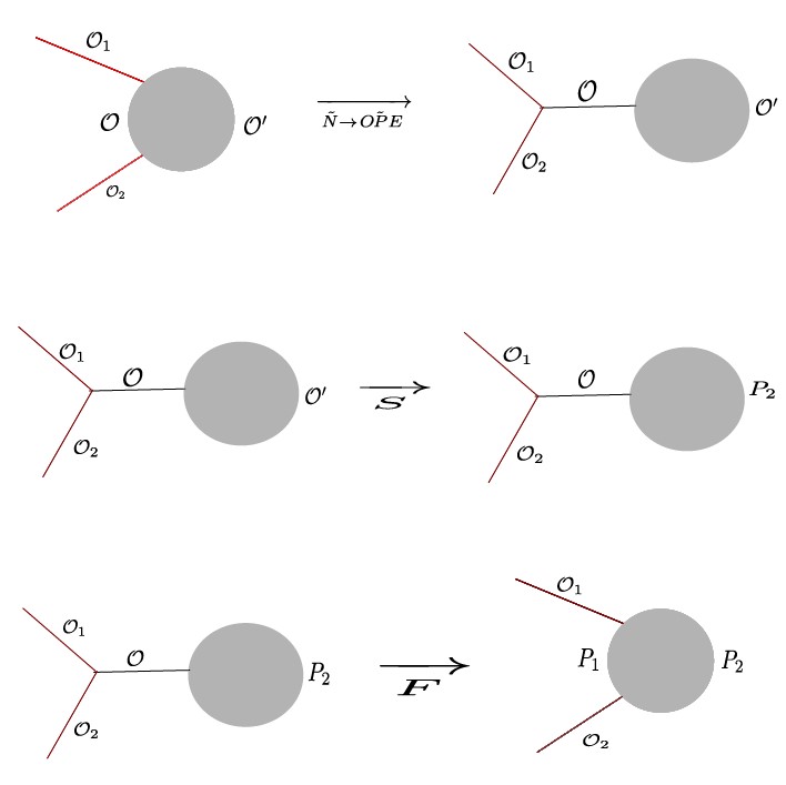
Figure 4: In the first step we transform from the $\tilde{N}$ channel to the $\widetilde{OPE}$ channel. Then we use the modular crossing transformation. At last, we use the Virasoro fusion kernel to write the OPE channel in terms of the Necklace channel.

$$\begin{split}\mathcal{F}^{\tilde{N}}_{hh^{\prime}}&=\widetilde{\mathcal{F}^{OPE}_{P^{\prime}P}}\,,\\ &=\int\frac{dP_{2}}{2}\frac{dP_{1}}{2}\mathbb{S}_{P^{\prime}P_{2}}[P]\,\mathbb{F}_{P,P_{1}}\begin{bmatrix}\tilde{P}&P_{2}\\ \tilde{P}&P_{2}\end{bmatrix}\mathcal{F}^{N}_{P_{1},P_{2}}\,.\end{split}$$ (156)

Now we know that the fusion kernel can be written in the following integral form Ghosh:2019rcj ,

$$\mathbb{F}_{P^{\prime\prime},P}\begin{bmatrix}P^{*}&\tilde{P}\\ P^{*}&\tilde{P}\end{bmatrix}=P(\alpha_{i};\alpha^{\prime\prime},\alpha)P(\alpha_{i};Q-\alpha^{\prime\prime},Q-\alpha)\int_{\mathcal{C}^{\prime}}\frac{ds}{i}\prod_{k=1}^{4}\frac{\mathcal{S}_{b}(s+U_{k})}{\mathcal{S}_{b}(s+V_{k})}$$ (157)

where,

$$P(\alpha_{i};\alpha^{\prime\prime},\alpha)=\frac{\Gamma_{b}^{2}(\alpha^{\prime\prime}+\alpha^{*}-\tilde{\alpha})\Gamma(\alpha^{\prime\prime}+Q-\tilde{\alpha}-\alpha^{*})\Gamma(\alpha^{\prime\prime}-Q+\tilde{\alpha}+\alpha^{*})\Gamma_{b}(2\alpha)}{\Gamma_{b}^{2}(\alpha)\Gamma(\alpha+Q-2\tilde{\alpha})\Gamma(\alpha-Q+2\alpha^{*})\Gamma_{b}(2\alpha-Q)}$$ (158)

along with,

$$\mathcal{S}_{b}(x):=\frac{\Gamma_{b}(x)}{\Gamma_{b}(Q-x)}.$$ (159)

We also define $U_{k}$ and $V_{k}$ as follows,

$$\begin{split}&U_{1}=i(P_{1}-P_{4})=0\,,\hskip 85.35826ptV_{1}=Q/2+i(-P^{\prime\prime}+P^{*}-\tilde{P})\,,\\ &U_{2}=-i(P_{1}+P_{4})=-2i\tilde{P}\,,\hskip 59.75095ptV_{2}=Q/2+i(P^{\prime\prime}+P^{*}-\tilde{P})\,,\\ &U_{3}=i(P_{2}+P_{3})=2iP^{*}\,,\hskip 65.44142ptV_{3}=Q/2+iP\,,\\ &U_{4}=i(P_{2}-P_{3})=0\,,\hskip 85.35826ptV_{4}=Q/2-iP\,.\end{split}$$ (160)

Various limits of the fusion kernel with heavy operator insertions are discussed in Collier:2019weq .
Now we will proceed to show the formalism to compute the Virasoro torus two-point function. If we insert the operator in the dual Necklace channel (Euclidean time circle), this can be written as,

$$\begin{split}\langle\mathcal{O}_{1}^{s}(v,\bar{v})\mathcal{O}_{2}^{s}(0)\rangle_{T^{2}(\tau,\bar{\tau})}&=\begin{minipage}[h]{21.68231pt} \vspace{-3 pt}\scalebox{0.3}{\includegraphics{yan_final.jpg}}\end{minipage}\\ &=\sum_{p,q}\begin{minipage}[h]{21.68231pt} \vspace{-9 pt}\scalebox{0.3}{\includegraphics{torus1.png}}\end{minipage}\\ &=\sum_{p,q}C_{\mathcal{O}_{1}\mathcal{O}_{p}\mathcal{O}_{q}}C_{\mathcal{O}_{2}\mathcal{O}_{p}\mathcal{O}_{q}}|\mathcal{F}^{g=1}_{12}(h_{p},h_{q};\tau,v)|^{2}\,.\end{split}$$ (161)

Considering the probe operators $\mathcal{O}_{1}=\mathcal{O}_{2}=\tilde{\mathcal{O}}$ to be heavy, we can write (161) as,

$$=\sum_{p,q}|C_{\tilde{\mathcal{O}}\mathcal{O}_{p}\mathcal{O}_{q}}|^{2}|\mathcal{F}^{g=1}_{12}(h_{p},h_{q};\tau,v)|^{2}\,.$$

Now the average over the product of two torus two-point function is given by Yan:2023rjh :

$$\begin{split}&\overline{\langle\mathcal{O}_{1}(v,\bar{v})\mathcal{O}_{2}(0)\rangle_{T^{2}(\tau,\bar{\tau})}{\langle\mathcal{O}_{1}(v^{\prime},\bar{v^{\prime}})\mathcal{O}_{2}(0)\rangle_{T^{2}(\tau^{\prime},\bar{\tau^{\prime}})}}}\,,\\ &=\sum_{p,q,g,h}\overline{|C_{\mathcal{O}_{1}\mathcal{O}_{p}\mathcal{O}_{q}}|^{2}|C_{\mathcal{O}_{1}\mathcal{O}_{g}\mathcal{O}_{h}}|^{2}}|\mathcal{F}^{\tilde{N},g=1}_{12}(h_{p},h_{q};\tau,v)|^{2}|\mathcal{F}^{\tilde{N},g=1}_{12}(h_{g},h_{h};\tau,v)|^{2}\,,\\ &=2\Bigg{|}\int dh_{p}dh_{q}\rho_{0}(h_{p})\rho_{0}(h_{q})C_{0}(\tilde{h},h_{p},h_{q})C_{0}(\bar{\tilde{h}},\bar{h}_{p},\bar{h}_{q})|\mathcal{F}^{\tilde{N},g=1}_{12}(h_{p},h_{q};\tau,v)|^{2}\Bigg{|}^{2}\end{split}$$ (162)

where

$$\mathcal{F}^{\tilde{N},g=1}_{12}(h,h^{\prime};\tau,v)=\int\frac{dP_{2}}{2}\frac{dP_{1}}{2}\mathbb{S}_{P^{\prime}P_{2}}[P]\,\mathbb{F}_{P,P_{1}}\begin{bmatrix}\tilde{P}&P_{2}\\ \tilde{P}&P_{2}\end{bmatrix}\mathcal{F}^{N}_{P_{1},P_{2}}.$$

and

$$C_{0}(P_{1},P_{2},P_{3})=\frac{\Gamma_{b}(2Q)\Gamma_{b}(\frac{Q}{2}\pm iP_{1}\pm iP_{2}\pm iP_{3})}{\sqrt{2}\Gamma_{b}(Q)^{3}\prod_{k=1}^{3}\Gamma_{b}(Q\pm 2iP_{k})}.$$ (163)

In (162) the “bar" denotes the averaging over the dimensions of the heavy operators while the other conformal dimensions are held fixed. The Liouville structure constants show a universal behaviour in this limit Collier:2018exn .

Fusion matrix in super Liouville field theory

We describe the fusion matrix in SLFT in this appendix . Generally, the fusion matrices take the following form $\{i,j\}=1,2$ which correspond to parity of even and odd respectively ,

$$\begin{split}&\mathbb{F}_{\alpha_{s},\alpha_{t}}\left[\begin{array}[]{cc}\alpha_{3}&\alpha_{2}\\ \alpha_{4}&\alpha_{1}\end{array}\right]^{i}_{j}={\Gamma_{i}(2Q-\alpha_{t}-\alpha_{2}-\alpha_{3})\Gamma_{i}(Q-\alpha_{t}+\alpha_{3}-\alpha_{2})\Gamma_{i}(Q+\alpha_{t}-\alpha_{2}-\alpha_{3})\Gamma_{i}(\alpha_{3}+\alpha_{t}-\alpha_{2})\over\Gamma_{j}(2Q-\alpha_{1}-\alpha_{s}-\alpha_{2})\Gamma_{j}(Q-\alpha_{s}-\alpha_{2}+\alpha_{1})\Gamma_{j}(Q-\alpha_{1}-\alpha_{2}+\alpha_{s})\Gamma_{j}(\alpha_{s}+\alpha_{1}-\alpha_{2})}\\ &\times{\Gamma_{i}(Q-\alpha_{t}-\alpha_{1}+\alpha_{4})\Gamma_{i}(\alpha_{1}+\alpha_{4}-\alpha_{t})\Gamma_{i}(\alpha_{t}+\alpha_{4}-\alpha_{1})\Gamma_{i}(\alpha_{t}+\alpha_{1}+\alpha_{4}-Q)\over\Gamma_{j}(Q-\alpha_{s}-\alpha_{3}+\alpha_{4})\Gamma_{j}(\alpha_{3}+\alpha_{4}-\alpha_{s})\Gamma_{j}(\alpha_{s}+\alpha_{4}-\alpha_{3})\Gamma_{j}(\alpha_{s}+\alpha_{3}+\alpha_{4}-Q)}\\ &\times{\Gamma_{\rm NS}(2Q-2\alpha_{s})\Gamma_{\rm NS}(2\alpha_{s})\over\Gamma_{\rm NS}(Q-2\alpha_{t})\Gamma_{\rm NS}(2\alpha_{t}-Q)}{1\over i}\int_{-i\infty}^{i\infty}d\tau J_{\alpha_{s},\alpha_{t}}\left[\begin{array}[]{cc}\alpha_{3}&\alpha_{2}\\ \alpha_{4}&\alpha_{1}\end{array}\right]^{i}_{j}\,,\end{split}$$ (164)

We will consider $i=j=1$, for the fusion matrix in NS sector. we have,

$$\begin{split}&J_{\alpha_{s},\alpha_{t}}\left[\begin{array}[]{cc}\alpha_{3}&\alpha_{2}\\ \alpha_{4}&\alpha_{1}\end{array}\right]^{1}_{1}={S_{NS}(Q+\tau-\alpha_{1})S_{\rm NS}(\tau+\alpha_{4}+\alpha_{2}-\alpha_{3})S_{NS}(\tau+\alpha_{1})S_{NS}(\tau+\alpha_{4}+\alpha_{2}+\alpha_{3}-Q)\over S_{NS}(Q+\tau+\alpha_{4}-\alpha_{t})S_{NS}(\tau+\alpha_{4}+\alpha_{t})S_{NS}(Q+\tau+\alpha_{2}-\alpha_{s})S_{NS}(\tau+\alpha_{2}+\alpha_{s})}\\ &+{S_{R}(Q+\tau-\alpha_{1})S_{R}(\tau+\alpha_{4}+\alpha_{2}-\alpha_{3})S_{R}(\tau+\alpha_{1})S_{R}(\tau+\alpha_{4}+\alpha_{2}+\alpha_{3}-Q)\over S_{R}(Q+\tau+\alpha_{4}-\alpha_{t})S_{R}(\tau+\alpha_{4}+\alpha_{t})S_{R}(Q+\tau+\alpha_{2}-\alpha_{s})S_{R}(\tau+\alpha_{2}+\alpha_{s})}\,,\end{split}$$ (165)

where $S_{NS,R}$ are defined by,

$$S_{NS}(x)=\frac{\Gamma_{NS}(x)}{\Gamma_{NS}(Q-x)},\hskip 56.9055ptS_{R}(x)=\frac{\Gamma_{R}(x)}{\Gamma_{R}(Q-x)}\leavevmode\nobreak\ \leavevmode\nobreak\ \leavevmode\nobreak\ \leavevmode\nobreak\ \leavevmode\nobreak\ \leavevmode\nobreak\ \textrm{with}\leavevmode\nobreak\ \leavevmode\nobreak\ \leavevmode\nobreak\ \leavevmode\nobreak\ \Gamma_{R}(x)=\Gamma_{b}(\frac{x+b}{2})\Gamma_{b}(\frac{x+b^{-1}}{2})$$ (166)

Alternatively, it can be shown that for $\alpha_{s}=0$, the fusion matrix takes the following form,

$$\begin{split}F_{0,\alpha_{t}}\left[\begin{array}[]{cc}\alpha_{3}&\alpha_{1}\\ \alpha_{3}&\alpha_{1}\end{array}\right]^{1}_{1}=C_{NS}(\alpha_{t},\alpha_{1},\alpha_{3}){W_{NS}(Q)W_{NS}(\alpha_{t})\over\pi W_{NS}(Q-\alpha_{1})W_{NS}(Q-\alpha_{3})}\,.\end{split}$$ (167)

One can also verify that,

$$W_{NS}(x)W_{NS}(Q-x)=-4\sin\pi b(x-Q/2)\sin\pi{1\over b}(x-Q/2)\,.$$ (168)

Appendix D Different transformations

We have the following basic moves Collier:2023fwi :

• Braiding:

  $$\leavevmode\hbox to78.02pt{\vbox to62.66pt{\text{[drawing]}}}\ =\mathbb{B}_{12}^{3}\ \leavevmode\hbox to78.02pt{\vbox to62.66pt{\text{[drawing]}}}$$ (169)

• Fusion:

  $$\leavevmode\hbox to113.87pt{\vbox to88.26pt{\text{[drawing]}}}\ =\sum_{s}\ \mathbb{F}_{st}\begin{bmatrix}3&2\\ 4&1\end{bmatrix}\ \leavevmode\hbox to113.87pt{\vbox to88.26pt{\text{[drawing]}}} s t s t$$ (170)

• Modular S-transformation:

  $$\leavevmode\hbox to78.02pt{\vbox to88.26pt{\text{[drawing]}}}\ =\sum_{2}\mathbb{S}_{12}[0]\ \leavevmode\hbox to78.02pt{\vbox to88.26pt{\text{[drawing]}}}$$ (171)

$\mathbb{B}$ is easy to determine,

$$\mathbb{B}_{12}^{3}=\pm\mathrm{e}^{\pi i(\Delta_{3}-\Delta_{1}-\Delta_{2})}\,.$$ (172)

References

- (1) R. Jackiw, Lower Dimensional Gravity, Nucl. Phys. B 252 (1985) 343–356.
- (2) C. Teitelboim, Gravitation and Hamiltonian Structure in Two Space-Time Dimensions, Phys. Lett. B 126 (1983) 41–45.
- (3) P. Saad, S. H. Shenker and D. Stanford, JT gravity as a matrix integral, 1903.11115.
- (4) J. M. Maldacena, The Large N limit of superconformal field theories and supergravity, Adv. Theor. Math. Phys. 2 (1998) 231–252 [hep-th/9711200].
- (5) E. Witten, Anti-de Sitter space and holography, Adv. Theor. Math. Phys. 2 (1998) 253–291 [hep-th/9802150].
- (6) G. J. Turiaci and E. Witten, = 2 JT supergravity and matrix models, JHEP 12 (2023) 003 [2305.19438].
- (7) L. V. Iliesiu, On 2D gauge theories in Jackiw-Teitelboim gravity, 1909.05253.
- (8) L. V. Iliesiu and G. J. Turiaci, The statistical mechanics of near-extremal black holes, JHEP 05 (2021) 145 [2003.02860].
- (9) L. V. Iliesiu, J. Kruthoff, G. J. Turiaci and H. Verlinde, JT gravity at finite cutoff, SciPost Phys. 9 (2020) 023 [2004.07242].
- (10) S. Collier, L. Eberhardt, B. Muehlmann and V. A. Rodriguez, The Virasoro minimal string, SciPost Phys. 16 (2024), no. 2, 057 [2309.10846].
- (11) S. Ebert, H.-Y. Sun and Z. Sun, -deformed free energy of the Airy model, JHEP 08 (2022) 026 [2202.03454].
- (12) A. Bhattacharyya, S. Ghosh and S. Pal, Aspects of deformed 2D topological gravity : from partition function to late-time SFF, 2309.16658.
- (13) M. Atiyah, Topological quantum field theories, Inst. Hautes Etudes Sci. Publ. Math. 68 (1989) 175–186.
- (14) V. Mikhaylov, Teichmüller TQFT vs. Chern-Simons theory, JHEP 04 (2018) 085 [1710.04354].
- (15) A. Maloney and E. Witten, Quantum Gravity Partition Functions in Three Dimensions, JHEP 02 (2010) 029 [0712.0155].
- (16) X. Yin, Partition Functions of Three-Dimensional Pure Gravity, Commun. Num. Theor. Phys. 2 (2008) 285–324 [0710.2129].
- (17) E. Witten, Three-Dimensional Gravity Revisited, 0706.3359.
- (18) J. Manschot, AdS(3) Partition Functions Reconstructed, JHEP 10 (2007) 103 [0707.1159].
- (19) A. Maloney and E. Witten, Averaging over Narain moduli space, JHEP 10 (2020) 187 [2006.04855].
- (20) S. Collier and A. Maloney, Wormholes and spectral statistics in the Narain ensemble, JHEP 03 (2022) 004 [2106.12760].
- (21) N. Afkhami-Jeddi, H. Cohn, T. Hartman and A. Tajdini, Free partition functions and an averaged holographic duality, JHEP 01 (2021) 130 [2006.04839].
- (22) N. Benjamin, C. A. Keller, H. Ooguri and I. G. Zadeh, Narain to Narnia, Commun. Math. Phys. 390 (2022), no. 1, 425–470 [2103.15826].
- (23) J. Chandra, S. Collier, T. Hartman and A. Maloney, Semiclassical 3D gravity as an average of large-c CFTs, JHEP 12 (2022) 069 [2203.06511].
- (24) A. Belin and J. de Boer, Random statistics of OPE coefficients and Euclidean wormholes, Class. Quant. Grav. 38 (2021), no. 16, 164001 [2006.05499].
- (25) T. G. Mertens, J. Simón and G. Wong, A proposal for 3d quantum gravity and its bulk factorization, JHEP 06 (2023) 134 [2210.14196].
- (26) L. Eberhardt, M. R. Gaberdiel and R. Gopakumar, Deriving the AdS3/CFT2 correspondence, JHEP 02 (2020) 136 [1911.00378].
- (27) L. Eberhardt, M. R. Gaberdiel and R. Gopakumar, The Worldsheet Dual of the Symmetric Product CFT, JHEP 04 (2019) 103 [1812.01007].
- (28) S. Collier, L. Eberhardt and M. Zhang, Solving 3d gravity with Virasoro TQFT, SciPost Phys. 15 (2023), no. 4, 151 [2304.13650].
- (29) S. Collier, L. Eberhardt and M. Zhang, 3d gravity from Virasoro TQFT: Holography, wormholes and knots, 2401.13900.
- (30) A. Dymarsky and A. Shapere, Bulk derivation of TQFT gravity, 2405.20366.
- (31) J. de Boer, D. Liska and B. Post, Multiboundary wormholes and OPE statistics, 2405.13111.
- (32) D. L. Jafferis, L. Rozenberg and G. Wong, 3d Gravity as a random ensemble, 2407.02649.
- (33) L. Chen, L.-Y. Hung, Y. Jiang and B.-X. Lao, Quantum 2D Liouville Path-Integral Is a Sum over Geometries in AdS3 Einstein Gravity, 2403.03179.
- (34) R. Ducrocq, M. Rausch De Traubenberg and M. Valenzuela, A pedagogical discussion of four-dimensional supergravity in superspace, Mod. Phys. Lett. A 36 (2021), no. 16, 2130015 [2104.06671].
- (35) L. Eberhardt, Notes on crossing transformations of Virasoro conformal blocks, 2309.11540.
- (36) J. Ellegaard Andersen and R. Kashaev, A TQFT from Quantum Teichmüller Theory, Commun. Math. Phys. 330 (2014) 887–934 [1109.6295].
- (37) N. Aghaei, M. Pawelkiewicz and J. Teschner, Quantisation of super Teichmüller theory, Commun. Math. Phys. 353 (2017), no. 2, 597–631 [1512.02617].
- (38) N. Aghaei, M. K. Pawelkiewicz and M. Yamazaki, Towards Super Teichmüller Spin TQFT, Adv. Theor. Math. Phys. 26 (2022), no. 2, 245–294 [2008.09829].
- (39) A. Sen and B. Zwiebach, String Field Theory: A Review, 2405.19421.
- (40) E. Witten, Notes On Super Riemann Surfaces And Their Moduli, Pure Appl. Math. Quart. 15 (2019), no. 1, 57–211 [1209.2459].
- (41) F. A. Dolan and H. Osborn, Conformal four point functions and the operator product expansion, Nucl. Phys. B 599 (2001) 459–496 [hep-th/0011040].
- (42) A. I. Larkin and Y. N. Ovchinnikov, Quasiclassical Method in the Theory of Superconductivity, Journal of Experimental and Theoretical Physics (1969).
- (43) F. Haake, Quantum Signatures of Chaos. Springer Series in Synergetics. Springer, Berlin, 2010.
- (44) O. Bohigas, M. J. Giannoni and C. Schmit, Characterization of chaotic quantum spectra and universality of level fluctuation laws, Phys. Rev. Lett. 52 (1984) 1–4.
- (45) M. V. Berry, The Bakerian Lecture, 1987: Quantum Chaology, Proceedings of the Royal Society of London Series A 413 (Sept., 1987) 183–198.
- (46) L. D’Alessio, Y. Kafri, A. Polkovnikov and M. Rigol, From quantum chaos and eigenstate thermalization to statistical mechanics and thermodynamics, Adv. Phys. 65 (2016), no. 3, 239–362 [1509.06411].
- (47) P. Hosur, X.-L. Qi, D. A. Roberts and B. Yoshida, Chaos in quantum channels, JHEP 02 (2016) 004 [1511.04021].
- (48) A. Nahum, S. Vijay and J. Haah, Operator Spreading in Random Unitary Circuits, Phys. Rev. X 8 (2018), no. 2, 021014 [1705.08975].
- (49) C. von Keyserlingk, T. Rakovszky, F. Pollmann and S. Sondhi, Operator hydrodynamics, OTOCs, and entanglement growth in systems without conservation laws, Phys. Rev. X 8 (2018), no. 2, 021013 [1705.08910].
- (50) I. L. Aleiner, L. Faoro and L. B. Ioffe, Microscopic model of quantum butterfly effect: out-of-time-order correlators and traveling combustion waves, Annals Phys. 375 (2016) 378–406 [1609.01251].
- (51) M. Gärttner, J. G. Bohnet, A. Safavi-Naini, M. L. Wall, J. J. Bollinger and A. M. Rey, Measuring out-of-time-order correlations and multiple quantum spectra in a trapped ion quantum magnet, Nature Phys. 13 (2017) 781 [1608.08938].
- (52) A. Kitaev, A simple model of quantum holography. https://online.kitp.ucsb.edu/online/entangled15/kitaev2/.
- (53) J. Maldacena and D. Stanford, Remarks on the Sachdev-Ye-Kitaev model, Phys. Rev. D 94 (2016), no. 10, 106002 [1604.07818].
- (54) J. Cotler, N. Hunter-Jones, J. Liu and B. Yoshida, Chaos, Complexity, and Random Matrices, JHEP 11 (2017) 048 [1706.05400].
- (55) D. Chowdhury and B. Swingle, Onset of many-body chaos in the model, Phys. Rev. D 96 (2017), no. 6, 065005 [1703.02545].
- (56) V. Khemani, D. A. Huse and A. Nahum, Velocity-dependent Lyapunov exponents in many-body quantum, semiclassical, and classical chaos, Phys. Rev. B 98 (2018), no. 14, 144304 [1803.05902].
- (57) A. Seshadri, V. Madhok and A. Lakshminarayan, Tripartite mutual information, entanglement, and scrambling in permutation symmetric systems with an application to quantum chaos, Phys. Rev. E 98 (2018), no. 5, 052205 [1806.00113].
- (58) K. Hashimoto, K. Murata and R. Yoshii, Out-of-time-order correlators in quantum mechanics, JHEP 10 (2017) 138 [1703.09435].
- (59) T. Ali, A. Bhattacharyya, S. S. Haque, E. H. Kim, N. Moynihan and J. Murugan, Chaos and Complexity in Quantum Mechanics, Phys. Rev. D 101 (2020), no. 2, 026021 [1905.13534].
- (60) A. Bhattacharyya, W. Chemissany, S. S. Haque, J. Murugan and B. Yan, The Multi-faceted Inverted Harmonic Oscillator: Chaos and Complexity, SciPost Phys. Core 4 (2021) 002 [2007.01232].
- (61) S. Sachdev and J. Ye, Gapless spin-fluid ground state in a random quantum Heisenberg magnet., Physical review letters 70 21 (1992) 3339–3342.
- (62) P. Di Francesco, P. H. Ginsparg and J. Zinn-Justin, 2-D Gravity and random matrices, Phys. Rept. 254 (1995) 1–133 [hep-th/9306153].
- (63) D. A. Roberts and D. Stanford, Two-dimensional conformal field theory and the butterfly effect, Phys. Rev. Lett. 115 (2015), no. 13, 131603 [1412.5123].
- (64) J. Maldacena, S. H. Shenker and D. Stanford, A bound on chaos, JHEP 08 (2016) 106 [1503.01409].
- (65) A. Kitaev and S. J. Suh, The soft mode in the Sachdev-Ye-Kitaev model and its gravity dual, JHEP 05 (2018) 183 [1711.08467].
- (66) A. M. García-García and J. J. M. Verbaarschot, Spectral and thermodynamic properties of the Sachdev-Ye-Kitaev model, Phys. Rev. D 94 (2016), no. 12, 126010 [1610.03816].
- (67) K. Papadodimas and S. Raju, Local Operators in the Eternal Black Hole, Phys. Rev. Lett. 115 (2015), no. 21, 211601 [1502.06692].
- (68) G. Sárosi, AdS2 holography and the SYK model, PoS Modave2017 (2018) 001 [1711.08482].
- (69) J. S. Cotler, G. Gur-Ari, M. Hanada, J. Polchinski, P. Saad, S. H. Shenker, D. Stanford, A. Streicher and M. Tezuka, Black Holes and Random Matrices, JHEP 05 (2017) 118 [1611.04650], [Erratum: JHEP 09, 002 (2018)].
- (70) V. Balasubramanian, B. Craps, B. Czech and G. Sárosi, Echoes of chaos from string theory black holes, JHEP 03 (2017) 154 [1612.04334].
- (71) C. Krishnan, S. Sanyal and P. N. Bala Subramanian, Quantum Chaos and Holographic Tensor Models, JHEP 03 (2017) 056 [1612.06330].
- (72) E. Dyer and G. Gur-Ari, 2D CFT Partition Functions at Late Times, JHEP 08 (2017) 075 [1611.04592].
- (73) V. Jahnke, Recent developments in the holographic description of quantum chaos, Adv. High Energy Phys. 2019 (2019) 9632708 [1811.06949].
- (74) N. R. Hunter-Jones, Chaos and Randomness in Strongly-Interacting Quantum Systems., Dissertation (Ph.D.), California Institute of Technology. 52 (2018) 1–4.
- (75) A. Altland, B. Post, J. Sonner, J. van der Heijden and E. P. Verlinde, Quantum chaos in 2D gravity, SciPost Phys. 15 (2023), no. 2, 064 [2204.07583].
- (76) A. Bhattacharyya, W. Chemissany, S. Shajidul Haque and B. Yan, Towards the web of quantum chaos diagnostics, Eur. Phys. J. C 82 (2022), no. 1, 87 [1909.01894].
- (77) J. Kudler-Flam, L. Nie and S. Ryu, Conformal field theory and the web of quantum chaos diagnostics, JHEP 01 (2020) 175 [1910.14575].
- (78) T. Zhou and B. Swingle, Operator growth from global out-of-time-order correlators, Nature Commun. 14 (2023), no. 1, 3411 [2112.01562].
- (79) B. Swingle, Unscrambling the physics of out-of-time-order correlators, Nature Phys. 14 (2018), no. 10, 988–990.
- (80) S. H. Shenker and D. Stanford, Black holes and the butterfly effect, JHEP 03 (2014) 067 [1306.0622].
- (81) D. Stanford, Many-body chaos at weak coupling, JHEP 10 (2016) 009 [1512.07687].
- (82) T. G. Mertens and G. J. Turiaci, Solvable models of quantum black holes: a review on Jackiw–Teitelboim gravity, Living Rev. Rel. 26 (2023), no. 1, 4 [2210.10846].
- (83) S. Xu and B. Swingle, Scrambling Dynamics and Out-of-Time-Ordered Correlators in Quantum Many-Body Systems, PRX Quantum 5 (2024), no. 1, 010201 [2202.07060].
- (84) I. García-Mata, R. A. Jalabert and D. A. Wisniacki, Out-of-time-order correlators and quantum chaos, Scholarpedia 18 (2023) 55237 [2209.07965].
- (85) Y. Kusuki and M. Miyaji, Entanglement Entropy, OTOC and Bootstrap in 2D CFTs from Regge and Light Cone Limits of Multi-point Conformal Block, JHEP 08 (2019) 063 [1905.02191].
- (86) P. Caputa, Y. Kusuki, T. Takayanagi and K. Watanabe, Out-of-Time-Ordered Correlators in , Phys. Rev. D 96 (2017), no. 4, 046020 [1703.09939].
- (87) P. Caputa, T. Numasawa and A. Veliz-Osorio, Out-of-time-ordered correlators and purity in rational conformal field theories, PTEP 2016 (2016), no. 11, 113B06 [1602.06542].
- (88) B. Craps, S. Khetrapal and C. Rabideau, Chaos in CFT dual to rotating BTZ, JHEP 11 (2021) 105 [2107.13874].
- (89) S. Das, B. Ezhuthachan, A. Kundu, S. Porey, B. Roy and K. Sengupta, Out-of-Time-Order correlators in driven conformal field theories, JHEP 08 (2022) 221 [2202.12815].
- (90) Y. Sekino and L. Susskind, Fast Scramblers, JHEP 10 (2008) 065 [0808.2096].
- (91) R. H. Poghossian, Structure constants in the N=1 superLiouville field theory, Nucl. Phys. B 496 (1997) 451–464 [hep-th/9607120].
- (92) A. Artemev and V. Belavin, Torus one-point correlation numbers in minimal Liouville gravity, JHEP 02 (2023) 116 [2210.14568].
- (93) E. D’Hoker and D. H. Phong, The Geometry of String Perturbation Theory, Rev. Mod. Phys. 60 (1988) 917.
- (94) A. Borel and J.-P. Serre, Le théorème de Riemann-Roch, Bulletin de la Société Mathématique de France 86 (1958) 97–136.
- (95) L. Baulieu and M. P. Bellon, Beltrami Parametrization and String Theory, Phys. Lett. B 196 (1987) 142–150.
- (96) H. Verlinde, Conformal field theory, two-dimensional quantum gravity and quantization of Teichmüller space, Nuclear Physics B 337 (1990), no. 3, 652–680.
- (97) K. Alkalaev and V. Belavin, Large- superconformal torus blocks, JHEP 08 (2018) 042 [1805.12585].
- (98) C. Grosche, Selberg Supertrace Formula for Superriemann Surfaces, Analytic Properties of Selberg Superzeta Functions and Multiloop Contributions for the Fermionic String, Commun. Math. Phys. 133 (1990) 433–486.
- (99) P. H. Ginsparg, APPLIED CONFORMAL FIELD THEORY, in Les Houches Summer School in Theoretical Physics: Fields, Strings, Critical Phenomena. 9, 1988. hep-th/9108028.
- (100) L. Eberhardt, Off-shell Partition Functions in 3d Gravity, Commun. Math. Phys. 405 (2024), no. 3, 76 [2204.09789].
- (101) S. He, Conformal bootstrap to Rényi entropy in 2D Liouville and super-Liouville CFTs, Phys. Rev. D 99 (2019), no. 2, 026005 [1711.00624].
- (102) B. Ponsot and J. Teschner, Liouville bootstrap via harmonic analysis on a noncompact quantum group, hep-th/9911110.
- (103) M. Srednicki, Thermal fluctuations in quantized chaotic systems, J. Phys. A 29 (1996) L75–L79 [chao-dyn/9511001].
- (104) J. M. Deutsch, Quantum statistical mechanics in a closed system, Phys. Rev. A 43 (Feb, 1991) 2046–2049.
- (105) M. Rigol, V. Dunjko and M. Olshanii, Thermalization and its mechanism for generic isolated quantum systems, Nature 452 (2007) 854–858.
- (106) N. Benjamin, H. Ooguri, S.-H. Shao and Y. Wang, Light-cone modular bootstrap and pure gravity, Phys. Rev. D 100 (2019), no. 6, 066029 [1906.04184].
- (107) Y.-S. Myung, CORRELATION FUNCTION FOR N=1 SUPERCONFORMAL MODELS ON SUPERTORUS, Phys. Rev. D 40 (1989) 1980.
- (108) A. Belin, J. de Boer, D. L. Jafferis, P. Nayak and J. Sonner, Approximate CFTs and Random Tensor Models, 2308.03829.
- (109) J. M. Maldacena and L. Maoz, Wormholes in AdS, JHEP 02 (2004) 053 [hep-th/0401024].
- (110) K. B. Alkalaev and V. A. Belavin, Holographic duals of large-c torus conformal blocks, JHEP 10 (2017) 140 [1707.09311].
- (111) P. Suchanek, Elliptic recursion for 4-point superconformal blocks and bootstrap in N=1 SLFT, JHEP 02 (2011) 090 [1012.2974].
- (112) L. Hadasz, Z. Jaskolski and P. Suchanek, Recursion representation of the Neveu-Schwarz superconformal block, JHEP 03 (2007) 032 [hep-th/0611266].
- (113) A. Blommaert, T. G. Mertens and H. Verschelde, The Schwarzian Theory - A Wilson Line Perspective, JHEP 12 (2018) 022 [1806.07765].
- (114) D. Chorazkiewicz and L. Hadasz, Braiding and fusion properties of the Neveu-Schwarz super-conformal blocks, JHEP 01 (2009) 007 [0811.1226].
- (115) S. Ferrara, A. F. Grillo, G. Parisi and R. Gatto, Covariant expansion of the conformal four-point function, Nucl. Phys. B 49 (1972) 77–98 [Erratum: Nucl.Phys.B 53, 643–643 (1973)].
- (116) L. Iliesiu, F. Kos, D. Poland, S. S. Pufu, D. Simmons-Duffin and R. Yacoby, Bootstrapping 3D Fermions, JHEP 03 (2016) 120 [1508.00012].
- (117) K. Alkalaev and S. Mandrygin, Torus shadow formalism and exact global conformal blocks, JHEP 11 (2023) 157 [2307.12061].
- (118) V. Rosenhaus, Multipoint Conformal Blocks in the Comb Channel, JHEP 02 (2019) 142 [1810.03244].
- (119) A. Bagchi, A. Mehra and P. Nandi, Field Theories with Conformal Carrollian Symmetry, JHEP 05 (2019) 108 [1901.10147].
- (120) A. Bagchi, R. Basu, A. Mehra and P. Nandi, Field Theories on Null Manifolds, JHEP 02 (2020) 141 [1912.09388].
- (121) A. Bagchi, D. Grumiller and P. Nandi, Carrollian superconformal theories and super BMS, JHEP 05 (2022) 044 [2202.01172].
- (122) A. Bagchi, P. Nandi, A. Saha and Zodinmawia, BMS Modular Diaries: Torus one-point function, JHEP 11 (2020) 065 [2007.11713].
- (123) S. Collier, Y. Gobeil, H. Maxfield and E. Perlmutter, Quantum Regge Trajectories and the Virasoro Analytic Bootstrap, JHEP 05 (2019) 212 [1811.05710].
- (124) A. Ghosh, H. Maxfield and G. J. Turiaci, A universal Schwarzian sector in two-dimensional conformal field theories, JHEP 05 (2020) 104 [1912.07654].
- (125) S. Collier, A. Maloney, H. Maxfield and I. Tsiares, Universal dynamics of heavy operators in CFT2, JHEP 07 (2020) 074 [1912.00222].
- (126) C. Yan, More on torus wormholes in 3d gravity, JHEP 11 (2023) 039 [2305.10494].