Active Learning for Neural PDE Solvers

Abstract

Solving partial differential equations (PDEs) is a fundamental problem in engineering and science. While neural PDE solvers can be more efficient than established numerical solvers, they often require large amounts of training data that is costly to obtain. Active Learning (AL) could help surrogate models reach the same accuracy with smaller training sets by querying classical solvers with more informative initial conditions and PDE parameters. While AL is more common in other domains, it has yet to be studied extensively for neural PDE solvers. To bridge this gap, we introduce AL4PDE, a modular and extensible active learning benchmark. It provides multiple parametric PDEs and state-of-the-art surrogate models for the solver-in-the-loop setting, enabling the evaluation of existing and the development of new AL methods for PDE solving. We use the benchmark to evaluate batch active learning algorithms such as uncertainty- and feature-based methods. We show that AL reduces the average error by up to 71% compared to random sampling and significantly reduces worst-case errors. Moreover, AL generates similar datasets across repeated runs, with consistent distributions over the PDE parameters and initial conditions. The acquired datasets are reusable, providing benefits for surrogate models not involved in the data generation.

1 Introduction

Partial differential equations describe numerous physical phenomena such as fluid dynamics, heat flow, and cell growth. Because of the difficulty of obtaining exact solutions for PDEs, it is common to utilize numerical schemes to obtain approximate solutions. However, numerical solvers require a high temporal and spatial resolution to obtain sufficiently accurate numerical solutions, leading to high computational costs. This issue is further exacerbated in settings like parameter studies, inverse problems, or design optimization, where many iterations of simulations must be conducted. Thus, it can be beneficial to replace the numerical simulator with a surrogate model by training a neural network to predict the simulator outputs (Takamoto et al., 2022; Lippe et al., 2023; Brandstetter et al., 2021; Gupta & Brandstetter, 2023; Li et al., 2020b). In addition to being more efficient, neural surrogate models have other advantages, such as being end-to-end differentiable.

One of the main challenges of neural PDE surrogates is that their training data is often obtained from the same expensive simulators they are intended to ultimately replace. Hence, training a surrogate provides a computational advantage only if the generation of the training data set requires fewer simulations than will be saved during inference. Moreover, it is non-trivial to obtain training data for a diverse set of initial conditions and PDE parameters required to train a surrogate model with sufficient generalizability. For instance, contrary to training foundation models for text and images, foundation models for solving PDEs require targeted and expensive data generation to generalize well.

Active learning is a possible solution to these challenges as it might help to iteratively select a smaller number of the most informative and diverse training trajectories, thereby reducing the total number of simulations required to reach the same level of accuracy. Furthermore, AL may also improve the reliability of the surrogate models by covering challenging dynamical regimes with enough training data, which may otherwise be hard to find through hand-tuned input distributions. However, developing neural PDE solvers is a challenging problem for AL due to the complex regression tasks characterized by high-dimensional input and output spaces and time series data. While AL has been used extensively for other scientific ML domains such as material science (Lookman et al., 2019; Wang et al., 2022; Zaverkin et al., 2022; 2024), it has only been recently applied to PDEs in the context of physics-informed neural networks (PINNs; Wu et al. 2023a; Sahli Costabal et al. 2020; Aikawa et al. 2023), specific PDE domains (Pestourie et al., 2021; 2023), or direct prediction models (Li et al., 2023; 2020b). Hence, AL is still unexplored for a broader class of neural PDE solvers, which currently rely on extensive, brute-force numerical simulations to generate a sufficient amount of training data.

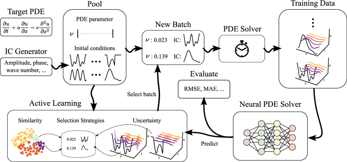
Figure 1: An extensible benchmark framework for pool-based active learning for neural PDE solvers.

Contributions.

This paper presents AL4PDE, the first AL framework for neural PDE solvers. The benchmark supports the study of existing AL algorithms in scientific ML applications and facilitates the development of novel PDE-specific AL methods. In addition to various AL algorithms, the benchmark provides differentiable numerical simulators for multiple PDEs, such as compressible Navier-Stokes, and neural surrogate models, such as the U-Net (Ronneberger et al., 2015; Gupta & Brandstetter, 2023). The benchmark is extensible, allowing new algorithms, models, and tasks to be added. Using the benchmark, we conducted several experiments exploring the behavior of AL algorithms for PDE solving. These experiments show that AL can increase data efficiency and especially reduce worst-case errors. Among the methods, the largest cluster maximum distance (LCMD) and stochastic batch active learning (SBAL) are consistently the two best-performing algorithms. We demonstrate that using AL can result in more accurate surrogate models trained in less time. Additionally, the generated data distribution is consistent between random repetitions, initial datasets, and models, showing that AL can reliably generate reusable datasets for neural PDE solvers that were not used to gather the data. The code will be available at github.com/dmusekamp/al4pde.

2 Background

We seek the solution $\operatorname{\mathbf{u}}:[0,T]\times\mathcal{X}\rightarrow\mathbb{R}^{N_{c}}$ of a PDE with a $D$-dimensional spatial domain $\mathcal{X}$, $\operatorname{\mathbf{x}}=[x_{1},x_{2},\ldots,x_{D}]^{\top}\in\mathcal{X}$, temporal domain $t\in[0,T]$, and ${N_{c}}$ field variables or channels $c$  (Brandstetter et al., 2021):

$$\partial_{t}\operatorname{\mathbf{u}}=F\left(\operatorname{\bm{\lambda}},t,\operatorname{\mathbf{x}},\operatorname{\mathbf{u}},\partial_{\operatorname{\mathbf{x}}}\operatorname{\mathbf{u}},\partial_{\operatorname{\mathbf{x}}\operatorname{\mathbf{x}}}\operatorname{\mathbf{u}},\ldots\right),\quad\quad\quad\quad\quad\quad\quad(t,\operatorname{\mathbf{x}})\in[0,T]\times\mathcal{X}$$ (1)

$$\operatorname{\mathbf{u}}(0,\operatorname{\mathbf{x}})=\operatorname{\mathbf{u}}^{0}(\operatorname{\mathbf{x}}),\quad\operatorname{\mathbf{x}}\in\mathcal{X};\quad\quad\mathcal{B}[\operatorname{\mathbf{u}}](t,\operatorname{\mathbf{x}})=0,\quad(t,\operatorname{\mathbf{x}})\in[0,T]\times\partial\mathcal{X}$$ (2)

Here, the boundary condition $\mathcal{B}$ (Eq. 2) determines the behavior of the solution at the boundaries $\partial\mathcal{X}$ of the spatial domain $\mathcal{X}$, and the initial condition (IC) $\operatorname{\mathbf{u}}^{0}$ defines the initial state of the system (Eq. 2). The vector $\operatorname{\bm{\lambda}}=(\operatorname{\lambda}_{1},...,\operatorname{\lambda}_{l})^{\top}\in\mathbb{R}^{l}$ with $\operatorname{\lambda}_{i}\in[a_{i},b_{i}]$ denotes the PDE parameters which influence the dynamics of the physical system governed by the PDE such as the diffusion coefficient in Burgers’ equation. In the following, we only consider a single boundary condition (periodic) for simplicity, and thus a single initial value problem can be identified by the tuple $\operatorname{\bm{\psi}}=(\operatorname{\mathbf{u}}^{0},\operatorname{\bm{\lambda}})$. The inputs to the initial value problem are drawn from the test input distribution $p_{T}$, $\operatorname{\bm{\psi}}\sim p_{T}(\operatorname{\bm{\psi}})=p_{T}(\operatorname{\mathbf{u}}^{0})p_{T}(\operatorname{\bm{\lambda}})$. The distributions are typically only given implicitly, i.e., we are given an IC generator $p_{T}(\operatorname{\mathbf{u}}^{0})$ and a PDE parameter generator $p_{T}(\operatorname{\bm{\lambda}})$, from which we can draw samples. For instance, the ICs may be drawn from a superposition of sinusoidal functions with random amplitudes and phases (Takamoto et al., 2022), while the PDE parameters ($\lambda_{i}$) are typically drawn uniformly from their interval $[a_{i},b_{i}]$.

The ground truth data is generated using a numerical solver, which can be defined as a forward operator $\mathcal{G}:\mathcal{U}\times\mathbb{R}^{l}\rightarrow\mathcal{U}$, mapping the solution at the current timestep to the one at the next timestep (Li et al., 2020b; Takamoto et al., 2022), $\operatorname{\mathbf{u}}(t+\Delta t,\cdot)=\mathcal{G}(\operatorname{\mathbf{u}}(t,\cdot),\operatorname{\bm{\lambda}})$ with timestep size $\Delta t$. Here, $\mathcal{U}$ is a suitable space of functions $\operatorname{\mathbf{u}}(t,\cdot)$. The solution $\operatorname{\mathbf{u}}$ is uniformly discretized across the spatial dimensions, yielding $N_{\operatorname{\mathbf{x}}}$ spatial points in total and the temporal dimension into $N_{t}$ timesteps. The forward operator is applied autoregressively, i.e., feeding the output state back into $\mathcal{G}$ (also called rollout), to obtain a full trajectory $\operatorname{\mathbf{u}}=(\operatorname{\mathbf{u}}^{0},\operatorname{\mathbf{u}}^{1},...,\operatorname{\mathbf{u}}^{N_{t}})$. We aim to replace the numerical solver with a neural PDE solver. While there are also other paradigms such as PINNs (Raissi et al., 2019), we restrict ourselves to autoregressive solvers $\mathcal{G}_{\theta}$ with $\hat{\operatorname{\mathbf{u}}}(t+\Delta t,\cdot)=\mathcal{G}_{\theta}(\hat{\operatorname{\mathbf{u}}}(t,\cdot),\operatorname{\bm{\lambda}})$ (Lippe et al., 2023). The training set for the said $\mathcal{G}_{\theta}(\operatorname{\mathbf{u}}(t,\cdot),\operatorname{\bm{\lambda}})$ consists of aligned pairs of $\operatorname{\bm{\psi}}$ and the corresponding solutions obtained from the numerical solver, i.e., $\operatorname{\mathcal{S}_{\text{train}}}=\{(\operatorname{\bm{\psi}}_{1},\operatorname{\mathbf{u}}_{1}),\ldots,(\operatorname{\bm{\psi}}_{N_{\text{train}}},\operatorname{\mathbf{u}}_{N_{\text{train}}})\}$. The neural network parameters $\theta$ are minimized using the root mean squared error (RMSE) on the training samples,

$$\mathcal{L}_{\text{RMSE}}(\operatorname{\mathbf{u}},\hat{\operatorname{\mathbf{u}}})=\sqrt{\frac{1}{N_{t}N_{\operatorname{\mathbf{x}}}N_{c}}\sum_{i=1}^{N_{t}}\sum_{j=1}^{N_{\operatorname{\mathbf{x}}}}\|{\operatorname{\mathbf{u}}(t_{i},\operatorname{\mathbf{x}}_{j})-\hat{\operatorname{\mathbf{u}}}(t_{i},\operatorname{\mathbf{x}}_{j})\|}_{2}^{2}}$$ (3)

where $\hat{\operatorname{\mathbf{u}}}$ denotes the estimated solutions of the neural surrogate models.

3 Related Work

Neural surrogate models for solving parametric PDEs is a popular area of research (Takamoto et al., 2023; Kapoor et al., 2023; Lippe et al., 2023; Hagnberger et al., 2024; Cho et al., 2024). Most existing works, however, often focus on single or uniformly sampled parameter values for the PDE coefficients and improving the neural architectures to boost the accuracy. In the context of neural PDE solvers, AL has primarily been applied to select the collocation points of PINNs. A typical approach is to sample the collocation points based on the residual error directly (Arthurs & King, 2021; Gao & Wang, 2023; Mao & Meng, 2023; Wu et al., 2023a). While this strategy can be effective, it differs from standard AL since it uses the “label”, i.e., the residual loss, when selecting data points. Aikawa et al. (2023) use a Bayesian PINN to select points based on uncertainty, whereas Sahli Costabal et al. (2020) employ a PINN ensemble for AL of cardiac activation mapping.

Pestourie et al. (2020) use AL to approximate Maxwell equations using ensemble-based uncertainty quantification for metamaterial design. Uncertainty-based AL was also employed for diffusion, reaction-diffusion, and electromagnetic scattering (Pestourie et al., 2023). In multi-fidelity AL, the optimal spatial resolution of the simulation is chosen (Li et al., 2020a; 2021; Wu et al., 2023b). For instance, Li et al. (2023) use an ensemble of FNOs in the single prediction setting. Wu et al. (2023c) apply AL to stochastic simulations using a spatio-temporal neural process. Bajracharya et al. (2024) investigate AL to predict the stationary solution of a diffusion problem. They consider AL using two different uncertainty estimation techniques and selecting based on the diversity in the input space. Pickering et al. (2022) use AL to find extreme events using ensembles of DeepONets (Lu et al., 2019). Next to using AL, it is also possible to reduce the data generation time using Krylov Subspace Recycling (Wang et al., 2023) or by applying data augmentation techniques such as Lie-point symmetries (Brandstetter et al., 2022). Such symmetries could also be combined with AL using LADA (Kim et al., 2021).

In recent years, several benchmarks for neural PDE solvers have been published (Takamoto et al., 2022; Gupta & Brandstetter, 2023; Hao et al., 2023; Luo et al., 2023; Liu et al., 2024). For instance, PDEBench (Takamoto et al., 2022) and PDEArena (Gupta & Brandstetter, 2023) provide efficient implementations of numerical solvers for multiple hydrodynamic PDEs such as Advection, Navier-Stokes, as well as recent implementations of neural PDE solvers (e.g., DilResNet, U-Net, FNO) for standard and conditioned PDE solving. Similarly, CODBench (Burark et al., 2023) compares the performance of different neural operators. WaveBench (Liu et al., 2024) is a benchmark specifically aimed at wave propagation PDEs that are categorized into time-harmonic and time-varying problems. For a more detailed discussion of related benchmarks, see Appendix A.3. Contrary to prior work, AL4PDE is the first framework for evaluating and developing AL methods for neural PDE solvers.

4 AL4PDE: An AL Framework for Neural PDE Solvers

The AL4PDE benchmark consists of three major parts: (1) AL algorithms, (2) surrogate models, and (3) PDEs and the corresponding simulators. It follows a modular design to make the addition of new approaches or problems as easy as possible (Fig. 2). The following sections describe the AL approaches, including the general problem setup, acquisition and similarity functions, and batch selection strategies. Moreover, we describe the included PDEs and surrogate models.

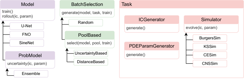
Figure 2: Structural overview of the AL4PDE benchmark.

4.1 Problem Definition and Setup

AL aims to select the most informative training samples so that the model can reach the same generalization error with fewer calls to the numerical solver. We measure the error using test trajectories on random samples from an input distribution $p_{T}$. Fig. 1 shows the full AL cycle. Since it requires retraining the NN(s) after each round, we use batch AL with sufficiently large batches. Specifically, in each round, a batch of simulator inputs $\operatorname{\mathcal{S}_{\text{batch}}}=\{\operatorname{\bm{\psi}}_{1},...,\operatorname{\bm{\psi}}_{N_{\text{batch}}}\}$ is selected. It is then passed to the numerical solver, which computes the output trajectories using numerical approximation schemes. The new trajectories are then added to the training set, and the cycle is repeated.

We implement pool-based active learning methods, which select from a set of possible inputs $\operatorname{\mathcal{S}_{\text{pool}}}=\{\operatorname{\bm{\psi}}_{1},...,\operatorname{\bm{\psi}}_{N_{\text{pool}}}\}$ called “pool”. The selected batch is then removed from the pool, simulated, and added to the training set $\operatorname{\mathcal{S}_{\text{train}}}$:

$$\operatorname{\mathcal{S}_{\text{pool}}}\leftarrow\operatorname{\mathcal{S}_{\text{pool}}}\setminus\operatorname{\mathcal{S}_{\text{batch}}},\quad\quad\ \operatorname{\mathcal{S}_{\text{train}}}\leftarrow\operatorname{\mathcal{S}_{\text{train}}}\cup\ \mathrm{solve}(\operatorname{\mathcal{S}_{\text{batch}}}).$$ (4)

We sample the pool set randomly from a proposal distribution $\pi$. In our experiments, we sample pool and test set from the same input distribution $\pi=p_{T}$, although $p_{T}$ might not always be known in practice. Following common practice, the initial batch is selected randomly. Besides pool-based methods, our framework is also compatible with query-synthesis AL methods that are not restricted to a finite pool set. Several principles are useful for the design of AL methods (Wu, 2018): First, they should select highly informative samples that allow the model to reduce its uncertainty. Second, selecting inputs that are representative of the test input distribution at test time is often desirable. Third, the batch should be diverse, i.e., the individual samples should provide non-redundant information. The last point is particular to the batch setting, which is essential to maintain acceptable runtimes. In the following, we will investigate batch AL methods that first extract latent features or direct uncertainty estimates from the neural surrogate model for each sample in the pool and subsequently apply a selection method to construct the batch.

4.2 Uncertainties and Features

Since neural PDE solvers provide high-dimensional autoregressive rollouts without direct uncertainty predictions, many AL methods cannot be applied straightforwardly. In the AL4PDE framework, we select the following two different classes of methods: the uncertainty-based approach, which directly assigns an uncertainty score to each candidate, and the feature-based framework of Holzmüller et al. (2023), which uses features (or kernels) to evaluate the similarity between inputs.

Uncertainties.

Epistemic uncertainty is often used as a measure of sample informativeness. While a more costly Bayesian approach is possible, we adopt the query-by-committee (QbC) approach (Seung et al., 1992), a simple but effective method that utilizes the variance between the ensemble members’ outputs as an uncertainty estimate:

$$a_{\text{QbC}}(\operatorname{\bm{\psi}}_{i}):=\frac{1}{N_{t}N_{\operatorname{\mathbf{x}}}N_{c}}\sum_{j=1}^{N_{t}}\sum_{k=1}^{N_{\operatorname{\mathbf{x}}}}\frac{1}{N_{m}}\sum_{m=1}^{N_{m}}\|{\hat{\operatorname{\mathbf{u}}}_{i,m}(t_{j},\operatorname{\mathbf{x}}_{k})-\overline{\hat{\operatorname{\mathbf{u}}}_{i}}(t_{j},\operatorname{\mathbf{x}}_{k})}\|_{2}^{2}\leavevmode\nobreak\ .$$ (5)

Here, $\overline{\hat{\operatorname{\mathbf{u}}}_{i}}$ is the mean prediction of all $N_{m}$ models with $\overline{\hat{\operatorname{\mathbf{u}}}_{i}}(t,\operatorname{\mathbf{x}})=\sum_{m}\hat{\operatorname{\mathbf{u}}}_{i,m}(t,\operatorname{\mathbf{x}})/N_{m}$. The ensemble members produce different outputs $\hat{\operatorname{\mathbf{u}}}_{i}$ due to the inherent randomness resulting from the weight initialization and stochastic gradient descent. The assumption of QbC is that the variance of the ensemble member predictions correlates positively with the error. A high variance, therefore, points to a region of the input space where we need more data. Using the variance of the model outputs directly corresponds to minimizing the expected MSE. Note that many more error metrics can be considered for PDEs (Takamoto et al., 2022), for which measures other than the variance may be more appropriate.

Features.

Many deep batch AL methods rely on some feature representation $\phi(\operatorname{\bm{\psi}})\in\mathbb{R}^{p}$ of inputs and utilize a distance metric in the feature space as a proxy for the similarity between inputs, which can help to ensure diversity of the selected batch. A typical representation is the inputs to the last neural network layer, but other representations are possible (Holzmüller et al., 2023). For neural PDE solvers, we compute the trajectory and concatenate the latent features at each timestep. Since this can result in very high-dimensional feature vectors, we follow Holzmüller et al. (2023) and apply Gaussian sketching. Specifically, we use $\phi_{\text{sketch}}(\operatorname{\bm{\psi}}):=\mathbf{U}\phi(\operatorname{\bm{\psi}})/\sqrt{p^{\prime}}\in\mathbb{R}^{p^{\prime}}$, to reduce the feature space to a fixed dimension $p^{\prime}$ using a random matrix $\mathbf{U}\in\mathbb{R}^{p^{\prime}\times p}$ with i.i.d. standard Gaussian entries.

While ensemble-based AL methods can also be formulated in terms of feature maps (Kirsch, 2023), the use of latent features allows AL methods to work with a single model. Moreover, methods based on distances of latent features can naturally incorporate diversity into batch AL by avoiding the selection of highly similar examples. Feature-based AL methods are, however, not translation equivariant. In settings with periodic boundary conditions, an IC translated along the spatial axis will produce a trajectory shifted by the same amount. By using periodic padding within the convolutional layers of U-Net, the network is equivariant w.r.t. translations; hence, adding a translated version of the same IC is redundant. Uncertainty-based approaches based on ensembles are translation-invariant since all ensemble model outputs are shifted by the same amount and produce the same outputs. To make feature-based AL translation invariant, we take the spatial average over the features.

4.3 Batch Selection Strategies

Given uncertainties or features, we need to define a method to select a batch of pool samples. As a generic baseline, we compare to the selection of a (uniformly) random sampling of the inputs according to the input distribution, $\operatorname{\bm{\psi}}\sim p_{T}(\operatorname{\bm{\psi}})$.

Uncertainty-based selection strategies.

When given a single-sample acquisition function $a$ such as the ensemble uncertainty, a simple and common approach to selecting a batch of $k$ samples is Top-K, taking the $k$ most uncertain samples. However, this does not ensure that the selected batch is diverse. To improve diversity, Kirsch et al. (2023) proposed stochastic batch active learning (SBAL). SBAL samples inputs $\operatorname{\bm{\psi}}$ from the remaining pool set $\operatorname{\mathcal{S}_{\text{pool}}}$ without replacement according to the probability distribution $p_{\text{power}}(\operatorname{\bm{\psi}})\propto a(\operatorname{\bm{\psi}})^{m}$, where $m$ is a hyperparameter controlling the sharpness of the distribution. Random sampling corresponds to $m=0$ and Top-K to $m=\infty$. The advantage of SBAL is that it selects samples from input regions that are not from the highest mode of the uncertainty distribution and encourages diversity.

Feature-based selection strategies.

In the simpler version of their Core-Set algorithm, Sener & Savarese (2018) iteratively select the input from the remaining pool with the highest distance to the closest selected or labeled point. While Core-Set produces batches of diverse and informative samples, its objective aims at covering the feature space uniformly. Hence, Core-Set in general does not select samples that are representative for the proposal distribution. To alleviate this issue, Holzmüller et al. (2023) propose to replace the greedy Core-Set with LCMD, a similarly efficient method inspired by k-medoids clustering. LCMD interprets previously selected inputs as cluster centers, assigns all remaining pool points to their closest center, selects the cluster with the largest sum of squared distances to the center, and from this cluster selects the point that is furthest away from the center. The newly selected point then becomes a new center and the process is repeated until a batch of the desired size is obtained.

4.4 PDEs

Figure 3: Example trajectories of the PDEs.

PDE	T in s	Sim. Res.	Train. Res.
		($N_{t},N_{\operatorname{\mathbf{x}}},[N_{\operatorname{\mathbf{y}}}]$)	($N_{t},N_{\operatorname{\mathbf{x}}},[N_{\operatorname{\mathbf{y}}}]$)
Burgers	2	(201, 1024)	(41, 256)
KS	40	(801, 512)	(41, 256)
CE	4	(501, 64)	(51, 64)
CNS	1	(21, 128, 128)	(21, 64, 64)

Table 1: Discretizations of the PDEs.

We consider 1D and 2D parametric PDEs, all with periodic boundary conditions. The first 1D PDE is the Burgers’ equation from PDEBench (Takamoto et al., 2022) with kinematic viscosity $\nu$: . Secondly, the Kuramoto–Sivashinsky (KS) equation, , from Lippe et al. (2023) demonstrates diverse dynamical behaviors, from fixed points and periodic limit cycles to chaos (Hyman & Nicolaenko, 1986). Next to the viscosity $\nu$, the domain length L is also varied. Thirdly, to test a multiphysics problem with more parameters, we include the so-called combined equation (CE) from Brandstetter et al. (2021) where we set the forcing term $\delta=0$: . Depending on the value of the PDE coefficients ($\alpha,\beta,\gamma$), this equation recovers the Heat, Burgers, or the Korteweg-de-Vries PDE. For 2D, we use the compressible Navier-Stokes (CNS) equations from PDEBench (Takamoto et al., 2022), $\definecolor{tcbcol@origin}{rgb}{0,0,0}\definecolor{.}{rgb}{0,0,0}\definecolor{.}{rgb}{0,0,0}\leavevmode\hbox to79.13pt{\vbox to12.85pt{\text{[drawing]}}},\leavevmode\nobreak\ \leavevmode\nobreak\ \leavevmode\nobreak\ \definecolor{tcbcol@origin}{rgb}{0,0,0}\definecolor{.}{rgb}{0,0,0}\definecolor{.}{rgb}{0,0,0}\leavevmode\hbox to208.85pt{\vbox to12.85pt{\text{[drawing]}}}$, . The ICs are generated from random initial fields. Full details on PDEs, ICs, and the PDE parameter distributions can be found in Appendix B.

4.5 Neural Surrogate Models

Currently, the benchmark includes the following neural PDE solvers: (i) a recent version of U-Net (Ronneberger et al., 2015) from Gupta & Brandstetter (2023), (ii) SineNet (Zhang et al., 2024), which is an enhancement of the U-Net model that corrects the feature misalignment issue in the residual connections of modern U-Nets and can be considered a model with state of the art accuracy, specifically for advection-type equations, and (iii) the Fourier neural operator  (FNO, Li et al., 2020b).

5 Selection of Experiments

We investigate (i) the impact of AL methods on the average error, (ii) the error distribution, (iii) the variance and reusability of the generated data, (iv) the temporal advantage of AL, and (v) conduct an ablation study concerning the different design choices of SBAL and LCMD. We use a smaller version of the modern U-Net from Gupta & Brandstetter (2023). We train the model on sub-trajectories (two steps) to strike a balance between learning auto-regressive rollouts and fast training. The training is performed with a cosine schedule, which reduces the learning rate from $10^{-3}$ to $10^{-5}$. The batch size is set to 512 (CNS: 64). We use an exponential data schedule, i.e., in each AL iteration, the amount of data added is equal to the current training set size (Kirsch et al., 2023). For 1D equations, we start with 256 trajectories (2D: 128). The pool size is fixed to 100,000 candidates. For Burgers, we choose the parameter space $\nu\in[0.001,1)$ and sample values uniformly at random but on a logarithmic scale. For the KS equation, besides the viscosity $\nu\in[0.5,4)$, we vary the domain length $L\in[0.1,100)$ as the second parameter. For CE, the parameter space is defined to be $\alpha\in[0,3)$, $\beta\in[0,0.4)$, $\gamma\in[0,1)$. For the CNS equations, we set $\eta,\zeta\in[10^{-4},10^{-1})$ and draw values on a logarithmic scale as with Burgers’ PDE. Additionally, we use random Mach numbers $m\in[0.1,1)$ for the IC generator. We repeat all experiments with five random seeds (Burgers: ten) and report the 95% confidence interval of the mean unless stated otherwise.

Comparison of AL methods.

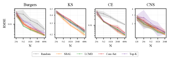
Figure 4: Error over the number of trajectories in the training set (N). The shaded area represents the $95\%$ confidence interval of the mean calculated over ten seeds for Burgers and and five for the rest. AL can reduce the error relative to random sampling of the inputs on all tested PDEs but CNS, where the difference was not significant.

Fig. 4 shows the RMSE for the various AL methods and PDEs. AL often reduces the error compared to sampling uniformly at random for the same amount of data. The advantage of AL is especially large for CE, which is likely due to the diverse dynamic regimes found in the PDE. SBAL and LCMD achieve similar errors on all PDEs with the exception of KS, where only SBAL can improve over random sampling. SBAL and LCMD can reach lower error values with only a quarter of the data points in the case of CE and Burgers. However, the greedy methods Top-K and Core-Set even increase the error for some PDEs. The difference on the CNS task was not significant, likely due to the performance of the base model training (see Fig. 8a) for a stronger model). Worst-case errors are of special interest when solving PDEs. Since we found the absolute maximum error to be unstable, we show the RMSE quantiles in Fig. 5. Notably, all AL algorithms reduce the higher quantiles while the 50 % percentile error is increased in some cases.

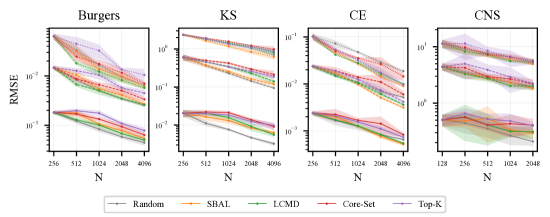
Figure 5: Error quantiles over the number of trajectories in the training set (N). The 50%, 95%, and 99% quantiles are displayed using full, dashed, and dotted lines, respectively. AL especially improves the higher error quantiles, making the trained model more reliable.

Different Error Functions.

It is important to consider error metrics for surrogate model training besides the RMSE (Takamoto et al., 2022). Thus, we explore the impact of AL on the mean absolute error (MAE) as an example of an alternative metric. As depicted in Fig. 7b), SBAL, when using the absolute difference between the models as the uncertainty, can also successfully reduce the MAE. However, the MAE does not improve greatly relative to random sampling when the standard variance between the models is used. Hence, it is crucial to tailor the AL method to the relevant metric.

Generated Datasets.

The marginal distributions of the PDE and the IC generator parameters implicitly sampled from by AL are shown in Fig. 6 for CE. These distributions are highly similar for different random seeds, and thus, AL reliably selects similar training datasets. The various AL methods generally sample similar parameter values but can differ substantially in certain regions of the parameter space (Section F.3). In general, the methods appear to sample more in the region of the chaotic KdV equation $(\alpha=3,\beta=0,\gamma=1)$. For $\alpha$ and $\gamma$, a difference between the two QbC methods Top-K and SBAL to the feature-based ones LCMD and Core-Set is observable. Appendix F provides the distributions for all PDEs and visual examples. To investigate the effect of the generated data on other models, we use an FNO ensemble to select the data that we use to train the standard U-Net. Fig. 7b) depicts the error of the U-Net over the number of samples selected using the FNO ensemble, showing the selected data is beneficial for models not used for the AL-based data selection. The reusability of the data is especially important, since otherwise the whole AL procedure would have to be repeated every time a new model is developed.

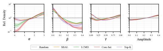
Figure 6: Marginal distribution of the PDE parameters and the amplitudes of the IC in the training set generated by AL for CE (relative to the uniform distribution). The shaded area represents the standard deviation between the random seeds. All AL methods exhibit a small standard deviation, indicating that they reliably generate similar datasets between independent runs.

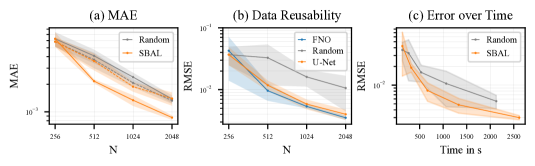
Figure 7: (a) AL with the MAE as the objective on Burgers, compared to the MAE of the same setup trained with the RMSE (dashed). Considering the desired error metric in the uncertainty estimate and training loss is essential. (b) Error of the standard U-Net on Burgers, with data generated using FNO or U-Net with SBAL. The selected data is also helpful for a model not used during AL. (c) Error of the standard U-Net on Burgers over the required total time. Using smaller FNOs to select the data, SBAL can provide smaller errors in the same amount of time.

Temporal Behavior.

The main experiments only provide the error over the number of data points since we use problems with rather fast solvers to accelerate the benchmarking of the AL methods. Second, a more lightweight model, trained for a shorter time, might be enough for data selection even if it does not reach the best possible accuracy. To investigate AL in terms of time efficiency gains, we perform one experiment on the Burgers’ PDE, for which the numerical solver is the most expensive among all 1D PDEs due to its higher resolution. We use SBAL with an ensemble of smaller FNOs (See Section C.6 for more details). We train a regular U-Net on the AL collected data, which allows us to use a small, lightweight model for data selection only and an expensive one to evaluate the data selected. Fig. 7c) shows the accuracy of the evaluation U-Net over the cumulative time consumed for training the selection model, selecting the inputs, and simulation. For the random baseline, only the simulation time is considered. On Burgers, AL provides better accuracy for the same time budget.

Ablations.

We ablate different design choices for the considered AL algorithms. For the SBAL algorithm, we investigate the base model architecture (Fig. 8a) and the ensemble size (Fig. 8b). On CNS, the accuracy of both SineNet and FNO can be significantly improved using SBAL, showing that AL is also helpful for other architectures. The improvement is even clearer than with the U-Net which did not show a statistically significant advantage. Consistent with prior work (Pickering et al., 2022), choosing an ensemble size of two models is already sufficient (Fig. 8b). In general, the average uncertainty and error of a trajectory with two ensemble members are correlated with a Pearson coefficient of 0.41 on CE in the worst case up to 0.94 on CNS (Table 8). Fig. 8c) compares different feature choices for the LCMD algorithm, which are used to calculate the distances. Using the spatial average of the last layer features produces higher accuracy than using the full feature vector or the features from the bottleneck step in the middle of the U-Net. Thus, it is indeed important for distance-based selection to consider the equivariances of the problem in the distance function.

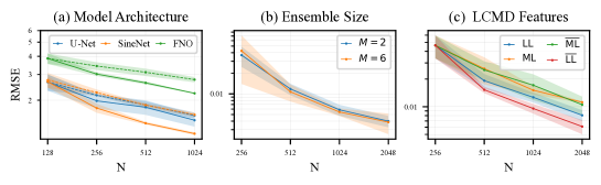
Figure 8: (a) Different base models on CNS using SBAL (solid) and random sampling (dashed). SBAL can also improve the accuracy of other models besides the U-Net. (b) Number of models $M$ in the ensemble on Burgers. SBAL works reliably with only two models. (c) Comparison of different feature vectors LCMD on CE. Shown are the last layer feature map (LL), its spatial average ($\overline{\text{LL}}$), as well as the features of the mid layer (ML) and its spatial average ($\overline{\text{ML}}$). Averaging the feature maps improves the error, indicating the importance of considering the model invariances.

6 Conclusion

This paper introduces AL4PDE, an extensible framework to develop and evaluate AL algorithms for neural PDE solvers. AL4PDE includes four PDEs, surrogate models including U-Net, FNO, and SineNet, and AL algorithms such as SBAL and LCMD. An initial study shows that existing AL algorithms can already be advantageous for neural PDE solvers and can allow a model to reach the same accuracy with up to four times fewer data points. Thus, our work shows the potential of AL for making neural PDE solvers more data-efficient and reliable for future application cases. However, the experiments also showed that stable model training can be difficult depending on the base architecture (CNS). AL is especially impacted by such issues, since the model is trained repeatedly with different data sets and the data selection relies on the model. Hence, more work on the reliability of the surrogate model training is necessary. Another general open issue of AL is the question of how to select hyperparameters which work sufficiently well on the growing, unseen datasets during AL. To be closer to realistic engineering applications, future work should also consider more complex geometries and non-periodic boundary conditions, as well as irregular grids. AL could be especially helpful in such settings due to the inherently more complex input space to select from.

  [sections] Active Learning for Neural PDE Solvers
Supplemental Material  [sections]l0

Appendix A Additional Background on Related Work

In this section, we elaborate on related works that tackle active learning in relevant settings and problems discussed here. Moreover, we summarize related work on uncertainty quantification and SciML benchmarks closely related to the proposed AL4PDE benchmark.

A.1 General Active Learning

Most AL algorithms are evaluated on classic image classification datasets (Ash et al., 2021; 2019) and many benchmarks also consider the more common classification setting (Rauch et al., 2023; Yang & Loog, 2018; Zhan et al., 2021). There is also work on specialized tasks such as entity matching (Meduri et al., 2020), structural integrity (Moustapha et al., 2022), material science (Wang et al., 2022), or drug discovery (Mehrjou et al., 2021). Holzmüller et al. (2023) present a benchmark for AL of single-output, tabular regression tasks. Wu et al. (2023a) study different adaptive and non-adaptive methods for selecting collocation points for PINNs. Ren et al. (2023) benchmark pool-based AL methods on simulated, mostly tabular regression tasks.

In terms of deep active learning methods for regression, there are multiple approaches: Query-by-committee (Seung et al., 1992) uses ensemble prediction variances as uncertainties. Tsymbalov et al. (2018) use Monte Carlo dropout to obtain uncertainties; however, their method is only applicable by training with dropout. Approaches based on last-layer Bayesian linear regression (Pinsler et al., 2019; Ash et al., 2021) are often convenient since they do not require ensembles or dropout. These methods are applicable in principle in our setting but lose their original Bayesian interpretation since the last layer of a neural operator is applied multiple times during the autoregressive rollout. Distance-based methods like Core-Set (Sener & Savarese, 2018; Geifman & El-Yaniv, 2017) and the clustering-based LCMD (Holzmüller et al., 2023) exhibit better runtime complexity than last-layer Bayesian methods while sharing their other advantages (Holzmüller et al., 2023). Since these algorithms just require some distance function between two input points, we can adapt them to the neural PDE solver setting in Section 4.2.

A.2 Uncertainty Quantification (UQ)

Uncertainty quantification has been studied in the context of SciML simulations. Psaros et al. (2023) provide a detailed overview of UQ methods in SciML, specifically for PINNs and DeepONets. However, effective and reliable UQ methods for neural operators (i.e., mapping between function spaces) and high dimensionality of data, which is common in PDE solving, remain challenging.

Neural PDE Solvers.

LE-PDE-UQ (Wu et al., 2024) deals with a method to estimate the uncertainty of neural operators by modeling the dynamics in the latent space. The model has been shown to outperform other UQ approaches, such as Bayes layer, Dropout, and L2 regularization on Navier-Stokes turbulent flow prediction tasks. Unlike the considered setting in our case, the model utilizes a history of 10 timesteps and has been tested only on a fixed PDE parameter. Hence, it is unclear whether the robustness of this approach remains when these settings change.

Mouli et al. (2024) aim to develop a cost-efficient method for uncertainty quantification of parametric PDEs, specifically one that works well in the out-of-domain test settings of PDE parameters. First, the study shows the challenges of existing UQ methods, such as the Bayesian neural operator (BayesianNO) for out-of-domain test data. It then shows that ensembling several neural operators is an effective strategy for UQ that is well-correlated with prediction errors and proposes diverse neural operators (DiverseNO) as a cost-effective way to estimate uncertainty with just a single model based on FNO outputting multiple predictions.

Thakur (2023) studies UQ in the context of neural operators and develops a probabilistic FNO model to quantify aleatoric and epistemic uncertainties. Weber et al. (2024) study UQ for FNO and propose a Laplace approximation for the Fourier layer to effectively compute uncertainty.

A.3 Further Scientific Machine Learning Benchmarks

In recent years, various benchmarks and datasets for SciML have been published. We outline some of the major open-source benchmarks below.

PDEBench (Takamoto et al., 2022) is a large-scale SciML benchmark of 1D to 3D PDE equations modeling hydrodynamics ranging from Burgers’ to compressible and incompressible Navier-Stokes equations. PDEArena (Gupta & Brandstetter, 2023) is a modern surrogate modeling benchmark including PDEs such as incompressible Navier-Stokes, Shallow Water, and Maxwell equations (Brandstetter et al., 2023). CFDBench (Luo et al., 2023) is a recent benchmark comprising four flow problems, each with three different operating parameters, the specific instantiations of which include varying boundary conditions, physical properties, and geometry of the fluid. The benchmark compares the generalization capabilities of a range of neural operators and autoregressive models for each of the said operating parameters. LagrangeBench (Toshev et al., 2023) is a large-scale benchmark suite for modeling 2D and 3D fluid mechanics problems based on the Lagrangian specification of the flow field. The benchmark provides both datasets and baseline models. For the former, it introduces seven datasets of varying Reynolds numbers by solving a weak form of NS equations using smoothed particle hydrodynamics. For the latter, efficient JAX implementations of GNN baseline models such as Graph Network-based Simulator and (Steerable) Equivariant GNN are included. EAGLE (Janny et al., 2023) introduces an industrial-grade dataset of non-steady fluid mechanics simulations encompassing 600 geometries and 1.1 million 2D meshes. In addition, to effectively process a dataset of this scale, the benchmark proposes an efficient multi-scale attention model, mesh transformer, to capture long-range dependencies in the simulation. BubbleML (Hassan et al., 2023) is a thermal simulations dataset comprising boiling scenarios that exhibit multiphase and multiphysics phase change phenomena. It also consists of a benchmark validating the dataset against U-Nets and several variants of FNO.

Appendix B Additional Problem Details

In the following section, we will discuss the tasks considered in detail. Table 1 shows the temporal and spatial resolution of the considered PDEs.

B.1 Burgers’ Equation

The 1D Burgers’ equation is written as

$$\partial_{t}u+u\partial_{x}u=({\nicefrac{{\nu}}{{\pi}}})\partial_{xx}u.$$ (6)

The spatial domain is set to $x\in[0,1]$. Following the parameter spacing of the PDE parameters values in PDEBench (Takamoto et al., 2022) and CAPE (Takamoto et al., 2023), we draw them on a logarithmic scale, i.e., we first draw $\operatorname{\bm{\lambda}}_{i,\text{normed}}$ uniformly from $[0,1)$ and then transform the parameter to its domain $[a_{i},b_{i})$ using

$$\operatorname{\bm{\lambda}}_{i}=a_{i}\exp(\log(b_{i}/a_{i})\operatorname{\bm{\lambda}}_{i,\text{normed}}).$$ (7)

We use the FDM-based JAX simulator and the initial condition generator from PDEBench (Takamoto et al., 2022). The ICs are constructed based on a superposition of sinusoidal waves (Takamoto et al., 2022),

$$\operatorname{\mathbf{u}}^{0}(x)=\sum_{i=1}^{N_{w}}A_{i}\sin(2\pi k_{i}x/L+\phi_{i})$$ (8)

where the wave number $k_{i}$ is an integer sampled uniformly from $[1,5)$, amplitude $A_{i}$ is sampled uniformly from $[0,1)$, and phase $\phi_{i}$ from $[0,2\pi)$. The number of waves $N_{w}$ is set to 2. Windowing is applied afterward with a probability of 10%, where all parts of the IC are set to zero outside of $[x_{L},x_{R}]$. $x_{L}$ is drawn uniformly from $[0.1,0.45)$ and $x_{R}$ from $[0.55,0.9)$. Lastly, the sign of $\operatorname{\mathbf{u}}^{0}$ is flipped for all entries with a probability of $10\%$.

B.2 Kuramoto-Sivashinsky (KS)

The 1D KS equation reads as

$$\partial_{t}u+u\partial_{x}u+\partial_{xx}u+\nu\partial_{xxxx}u=0\quad x\in[0,L].$$ (9)

The ICs are generated using the superposition of sinusoidal waves (Eq. 8), but $k_{i}$ is sampled from $[1,10)$, $A_{i}$ from $[-1,1)$ and $\phi_{i}$ from $[0,2\pi)$. No windowing or sign flips are applied. The total number of waves $N_{w}$ in this case is set to 10. Since we cannot omit the first part of the simulations as Lippe et al. (2023), we reduce the simulation time to 40s, but allow for more variance in the ICs to reach the chaotic behavior easier by increasing the number of wave functions of the IC. The trajectories are obtained using JAX-CFD (Dresdner et al., 2023). The PDE parameters are drawn uniformly from their range (no logarithmic scale).

B.3 Combined Equation (CE)

We adopt the combined equation albeit without the forcing term and the corresponding numerical solver from Brandstetter et al. (2021).

$$\partial_{t}u+\partial_{x}\left(\alpha u^{2}-\beta\partial_{x}u+\gamma\partial_{xx}u\right)=0$$ (10)

As for the IC, the domain of $k_{i}$ is set to $[1,3)$ and for $A_{i}$ it is set as $[-0.4,0.4)$. The number of waves $N_{w}$ is set to 5, and no windowing or sign flips are applied either. The PDE parameters are also drawn uniformly from their range. Depending on the choice of the PDE coefficients ($\alpha,\beta,\gamma$), this equation recovers the Heat (0, 1, 0), Burgers (0.5, 1, 0), or the Korteweg-de-Vries (3, 0, 1) PDE. The spatial domain is set to $x\in[0,16]$.

B.4 Compressible Navier-Stokes (CNS)

The 2D CNS equations from PDEBench (Takamoto et al., 2022) are written as

$$\partial_{t}\rho+\nabla\cdot(\rho\textbf{v}) =0,$$ (11a)

$$\rho(\partial_{t}\textbf{v}+\textbf{v}\cdot\nabla\textbf{v}) =-\nabla p+\eta\triangle\textbf{v}+(\zeta+{\nicefrac{{\eta}}{{3}}})\nabla(\nabla\cdot\textbf{v}),$$ (11b)

$$\partial_{t}(\epsilon+{\nicefrac{{\rho v^{2}}}{{2}}}) +\nabla\cdot[(p+\epsilon+{\nicefrac{{\rho v^{2}}}{{2}}})\bf{v}-\bf{v}\cdot\sigma^{\prime}]=0,$$ (11c)

where $\sigma^{\prime}$ is the viscous tensor. The equation has four channels (density $\rho$, velocity x-component $v_{x}$ and y-component $v_{y}$ as well as the pressure $p$. The spatial domain is set to $\operatorname{\mathbf{x}}\in[0,1]\times[0,1]$ We use the JAX simulator and IC generator from PDEBench (Takamoto et al., 2022) for CNS equations. The PDE parameters are drawn in logarithmic scale as in Eq. 7. The IC generator for the pressure, density, and velocity channels is also based on the superposition of sinusoidal functions. However, the velocity channels are renormalized so that the IC has a given input Mach number. Secondly, we constrain the density channel to be positive by

$$\operatorname{\mathbf{u}}_{\rho}=\rho_{0}(1+\Delta_{\rho}\operatorname{\mathbf{u}}_{\rho}^{\prime}/\max_{x}(|\operatorname{\mathbf{u}}_{\rho}^{\prime}(x)|)$$ (12)

where $\rho_{0}$ is sampled from $[0.1,10)$ and $\Delta_{\rho}$ from $[0.013,0.26)$. The pressure channel $p$ is similarly transformed using $\Delta_{p}\in[0.04,0.8)$. The offset $p_{0}$ is defined relatively to $\rho_{0}$ as $p_{0}=T_{0}\rho_{0}$ with $T_{0}\in[0.1,10)$. The compressibility is reduced using a Helmholtz-decomposition (Takamoto et al., 2022). A windowing is applied with a probability of $50\%$ to a channel.

Appendix C Additional Model and Training Details

This section describes the baseline surrogate models used in more detail, lists the hyperparameters, and explains various training methods. First, we provide a short description of the base models used. Then, we explain the training methods and list the hyperparameters.

C.1 Fourier Neural Operators (FNOs)

We use the FNO (Li et al., 2020b) implementation provided by PDEBench (Takamoto et al., 2022). FNOs are based on spectral convolutions, where the layer input is transformed using a Fast Fourier Transformation (FFT), multiplied in the Fourier space with a weight matrix, and then transformed back using an inverse FFT. Following the recent observations made in Lanthaler et al. (2023; 2024) that only a small fixed number of modes are sufficient to achieve the needed expressivity of FNO, we retain only a limited number of low-frequency Fourier modes and discard the ones with higher frequencies. The raw PDE parameter values are appended as additional constant channels to the model input (Takamoto et al., 2023).

C.2 U-shaped Networks (U-Nets)

U-Net (Ronneberger et al., 2015) is a common architecture in computer vision, particularly for perception and semantic segmentation tasks. The structure resembles an hourglass, where the inputs are first successively downsampled at multiple levels and then gradually, with the same number of levels, upsampled back to the original input resolution. This structure allows the model to capture and process spatial information at multiple scales and resolutions. The U-Net used in this paper is based on the modern U-Net version of Gupta & Brandstetter (2023), which differs from the original U-Net (Ronneberger et al., 2015) by including improvements such as group normalization (Wu & He, 2018). The model is conditioned on the input PDE parameter values, where they are transformed into vectors using a learnable Fourier embedding (Vaswani et al., 2017) and a projection layer and are then added to the convolutional layers’ inputs in the up and down blocks.

C.3 SineNet

U-Nets were originally designed for semantic segmentation problems in medical images (Ronneberger et al., 2015). Due to its intrinsic capabilities for multi-scale representation modeling, U-Nets have been widely adopted by the SciML community for PDE solving (Takamoto et al., 2022; Gupta & Brandstetter, 2023; Lippe et al., 2023; Rahman et al., 2022; Ovadia et al., 2023). One of the important components of U-Nets to recover high-resolution details in the upsampling path is by the fusion of feature maps using skip connections. This does not cause an issue for semantic segmentation tasks since the desired output for a given image is a segmentation mask. However, in the context of time-dependent PDE solving, specifically for advection-type PDEs modeling transport phenomena, this is not well-suited since there will be a “lag” in the feature maps of the downsampling path since the upsampling path is expected to predict the solution u for the next timestep. This detail was overlooked in U-Net adaptations for time-dependent PDE solving. SineNet is a recently introduced image-to-image model that aims to mitigate this problem by stacking several U-Nets, called waves, drastically reducing the feature misalignments. More formally, SineNet learns the mapping

$${\bm{x}_{t}} ={P}(\{{\bm{u}_{t-h+1},\ldots,\bm{u}_{t}}\})$$

$$\bm{u}_{t+1} ={Q}(\bm{x}_{t+1})$$

$$\bm{x}_{t+\Delta_{k}} ={V_{k}}(\bm{x}_{t-\Delta_{k-1}}),\quad\quad k=1,\ldots,K$$

Unlike the original SineNet, our adaptation uses only one temporal step as a context to predict the solution for the subsequent timestep.

C.4 Hyperparameters and Training Protocols

During AL, we use m=1 for power sampling and a prediction batch size for the pool of 200. The features of all inputs are projected using the sketch operator to a dimension of 512. Table 2 lists the model hyperparameters.

Table 2: Model hyperparamters.

U-Net
Activation	GELU (Hendrycks & Gimpel, 2016)
Conditioning	Fourier (Vaswani et al., 2017)
Channel multiplier	[1, 2, 2, 4]
Hidden Channels	16
# Param	3,378,865 (1D) / 9,182,036 (2D)
FNO
Activation	GELU (Hendrycks & Gimpel, 2016)
Conditioning	Additional input channel
Layers	4
Width	64 (1D) / 32 (2D)
Modes	20
# Param	353,154 (1D) / 3,286,310 (2D)
SineNet
Activation	GELU (Hendrycks & Gimpel, 2016)
Conditioning	Fourier (Vaswani et al., 2017)
Hidden Channels	32
Waves	4
# Param	5,020,840 (2D)

The inputs are channel-wise normalized using the standard deviation of the different channels on the initial data set. The outputs are denormalized accordingly. The input only consists of the current state $\textbf{u}_{t}$, not including data from prior timesteps. All models are used to predict the difference to the current timestep (for U-Net, the outputs are multiplied with a fixed factor of 0.3 following Lippe et al. (2023).

We employ one- and two-step training strategies during the training phase and a complete rollout of the trajectories during validation. For the FNO model in the 2D experiment we found it better to use the teacher-forcing schedule from Takamoto et al. (2023). We found it necessary to add gradient clipping to prevent a sudden divergence in the training curve. To account for the very different gradient norms among problems, we set the upper limit to 5 times the highest gradient found in the first five epochs. Afterwards, the limit is adapted using a moving average.

C.5 Hardware and Runtime

Table 3: Total runtime of the different AL methods and the memory during training (since all methods train the same model, the memory usage during training is identical).

	Burgers	KS	CE	CNS
Runtime in h
Random	15.1	12.9	16.8	37.9
SBAL	22.9	20.1	25.6	54.4
LCMD	14.5	13.9	17.2	39.0
Core-Set	14.5	13.4	16.6	39.7
Top-K	22.1	29.8	26.4	55.5
Training Memory in GB
All	8.16	8.18	4.47	7.29

The experiments were performed on NVIDIA GeForce RTX 4090 GPUs (one per experiment). Table 3 shows the runtime and GPU memory during training.

C.6 Timing Experiment

A realistic time measurement for the simulator of Burgers’ equation is challenging. Firstly, we observed that we can reach the shortest time per trajectory by setting the batch size to 4096 (0.52 seconds). Therefore, we use this as the fixed time per trajectory. The actual simulation times per AL iteration are higher since we start with batch sizes below this saturation point. Secondly, the simulation step size is adapted to the PDE parameter value due to the CFL condition (Lewy et al., 1928). Therefore, it would be beneficial to batch similar parameter values together and also to consider the parameter simulation costs in the acquisition function. Fig. 9 shows training, selection, and simulation times.

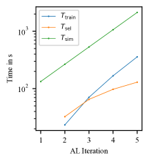
Figure 9: Cumulative training, selection, and simulation times necessary to reach the given active learning iteration (e.g., time to select data for iteration 2 counted in iteration 2) for 1D Burgers PDE.

The FNO surrogate used for selection is only trained for 20 epochs with a batch size of 1024. We use one-step training, and the learning rate of 0.001 is not annealed. The model itself has a width of 20 and uses 20 modes, resulting in 36,706 parameters. During selection, a batch size of 32,768 is used.

Appendix D Framework Overview

The framework has three major components: Model, BatchSelection, and Task. Task acts as a container of all the PDE-specific information and contains the Simulator, PDEParamGenerator, and ICGenerator classes. PDEParamGenerator and ICGenerator can draw samples from the test input distribution $p_{T}$. The inputs are first drawn from a normalized range and then transformed into the actual inputs. Afterward, the inputs can be passed to the simulator to be evolved into a trajectory. Fig. 10 shows the pseudocode of the (random) data generation pipeline. In order to implement a new PDE, a user has to implement a new subclass of Simulator overwrite the __call__ function and, if desired, add a new ICGenerator.

⬇

1

2class PDEParamGenerator:

3\pardef get_normed_pde_params(self, n):

4# Generates the random PDE parameters in a normed space

5# (e.g. between 0 and 1).

6\pardef get_pde_params(self, pde_params_normed):

7# Transforms the normed parameters to their true value.

8\par\parclass ICGenerator:

9\pardef initialize_ic_params(self, n):

10# Generates the random parameters of an IC (e.g. Mach number).

11\pardef generate_initial_conditions(self, ic_params, pde_params)

12# Transforms the IC parameters and PDE parameters to the IC.

13\par\parclass Simulator:

14\pardef __call__(self, ic, pde_params, grid):

15# Evolves the IC for a given PDE parameter.

16\par\par# generate pde parameters

17pde_params_normed = pde_gen.get_normed_pde_params(n)

18pde_params = pde_gen.get_pde_params(pde_params_normed)

19\par# generate ICs

20ic_params = ic_gen.initialize_ic_params(n)

21ic_gen.generate_initial_conditions(ic_params, pde_params)

22\partrajectories = sim(ic, pde_param, grid)

Figure 10: Interface and example code for generating inputs and simulation.

⬇

1

2class Model(nn.Module):

3\pardef init_training(self, al_iter):

4# Reset model, optimizer, scheduler, ...

5\pardef forward(self, xx, grid, param, return_features):

6# Predic next state.

7\pardef rollout(self, xx, grid, final_step, param, return_features):

8# Autoregressive rollout of the model until timestep final_step.

9\pardef evaluate(self, step, loader, prefix):

10# Evaluate the model on the given dataset (e.g. validation, train).

11\pardef train_single_epoch(self, current_epoch, total_epoch, num_epoch):

12# Train the model for one epoch.

13\pardef train_n_epoch(self, al_iter, num_epoch):

14# Train the model .

15\par\parclass ProbModel(Model):

16\pardef uncertainty(self, xx, grid, param):

17# Get uncertainty over next state.

18\pardef unc_roll_out(self, xx, grid, final_step, param, return_features):

19# Compute prediction and uncertainty of the rollout.

20\par\parclass BatchSelection:

21\pardef generate(self, prob_model, al_iter, train_loader):

22# Selects new inputs and passes them to the simulator.

23\par\parclass PoolBased(BatchSelection):

24\pardef select_next(self, step, prob_model, ic_pool, pde_param_pool,

25ic_train, pde_param_train, grid, al_iter):

26# Selects new input from (ic_pool, pde_param_pool).

27\par\parfor al_iter in range(num_al_iter):

28# retrain model

29prob_model.train_n_epoch(al_iter, num_epoch)

30\par# select next inputs

31batch_sel.generate(prob_model, al_iter, train_loader)

Figure 11: Interface and example code for the neural operator models and AL methods.

Fig. 11 shows the interface for the Model and ProbModel classes. Model provides functions to rollout a surrogate and deals with the training and evaluation. In order to add a new surrogate, a user has to overwrite the forward method. The rollout function also allows to get the internal model features for distance-based acquisition functions. ProbModel is an extension of the Model class, which adds the possibility of getting an uncertainty estimate. After training the model, the BatchSelection class is called in order to select a new set of inputs. The most important subclass is the PoolBased class, which deals with managing the pool and provides the select_next method, which a new pool-based method has to overwrite.

Appendix E Detailed Results

Tables 4, 5, 6 and 7 list the results from the main experiments. Table 8 shows the Pearson and Spearman coefficient of the average uncertainty per trajectory with the average error per trajectory. Among the PDEs, the Pearson correlation coefficient is the lowest on CE. The Spearman coefficient, which measures the correlation in terms of the ranking, is above 0.73 on average for all experiments.

Table 4: Error metrics on Burgers’ equation.

Iteration	1	2	3	4	5
RMSE $\times 10^{-2}$
Random	$3.684\pm 0.001$.203)	$3.278\pm 0.002$.107)	$1.607\pm 0.000$.485)	$1.062\pm 0.000$.614)	$0.552\pm 0.000$.133)
SBAL	$3.684\pm 0.001$.203)	$1.179\pm 0.000$.223)	$0.586(0.106)$	$0.400(0.075)$	$0.259\pm 0.000$.028)
LCMD	$3.684\pm 0.001$.203)	$0.808\pm 0.000$.053)	$0.521\pm 0.000$.052)	$0.394\pm 0.000$.043)	$0.269(0.014)$
Core-Set	$3.684\pm 0.001$.203)	$1.021(0.160)$	$0.659\pm 0.000$.100)	$0.476\pm 0.000$.134)	$0.292\pm 0.000$.015)
Top-K	$3.684\pm 0.001$.203)	$1.494\pm 0.000$.250)	$0.964\pm 0.000$.258)	$0.477\pm 0.000$.044)	$0.360\pm 0.000$.096)
50% Quantile $\times 10^{-2}$
Random	$0.182\pm 0.000$.015)	$0.122\pm 0.000$.015)	$0.083\pm 0.000$.010)	$0.058\pm 0.000$.005)	$0.044\pm 0.000$.007)
SBAL	$0.182\pm 0.000$.015)	$0.178\pm 0.000$.032)	$0.105\pm 0.000$.011)	$0.078\pm 0.000$.011)	$0.054\pm 0.000$.006)
LCMD	$0.182\pm 0.000$.015)	$0.129(0.014)$	$0.101(0.015)$	$0.068(0.008)$	$0.050(0.006)$
Core-Set	$0.182\pm 0.000$.015)	$0.169\pm 0.000$.017)	$0.133\pm 0.000$.013)	$0.094\pm 0.000$.014)	$0.063\pm 0.000$.008)
Top-K	$0.182\pm 0.000$.015)	$0.197\pm 0.000$.020)	$0.176\pm 0.000$.024)	$0.109\pm 0.000$.010)	$0.078\pm 0.000$.012)
95% Quantile $\times 10^{-2}$
Random	$1.468\pm 0.000$.136)	$0.834(0.125)$	$0.502\pm 0.000$.037)	$0.343\pm 0.000$.014)	$0.255\pm 0.000$.025)
SBAL	$1.468\pm 0.000$.136)	$1.054\pm 0.000$.248)	$0.544\pm 0.000$.065)	$0.409\pm 0.000$.064)	$0.269\pm 0.000$.026)
LCMD	$1.468\pm 0.000$.136)	$0.669\pm 0.000$.069)	$0.503(0.091)$	$0.347(0.030)$	$0.259(0.020)$
Core-Set	$1.468\pm 0.000$.136)	$0.865\pm 0.000$.123)	$0.662\pm 0.000$.090)	$0.503\pm 0.000$.113)	$0.336\pm 0.000$.034)
Top-K	$1.468\pm 0.000$.136)	$1.273\pm 0.000$.177)	$1.045\pm 0.000$.200)	$0.575\pm 0.000$.064)	$0.449\pm 0.000$.077)
99% Quantile $\times 10^{-2}$
Random	$6.315\pm 0.000$.838)	$3.327\pm 0.000$.724)	$1.653\pm 0.000$.111)	$0.968(0.046)$	$0.649\pm 0.000$.027)
SBAL	$6.315\pm 0.000$.838)	$3.169\pm 0.000$.945)	$1.360(0.213)$	$0.987\pm 0.000$.239)	$0.599(0.056)$
LCMD	$6.315\pm 0.000$.838)	$1.802\pm 0.000$.157)	$1.223\pm 0.000$.237)	$0.819\pm 0.000$.108)	$0.573\pm 0.000$.041)
Core-Set	$6.315\pm 0.000$.838)	$2.461(0.500)$	$1.756\pm 0.000$.360)	$1.153\pm 0.000$.295)	$0.703\pm 0.000$.056)
Top-K	$6.315\pm 0.000$.838)	$4.456\pm 0.001$.685)	$3.251\pm 0.001$.039)	$1.347\pm 0.000$.129)	$1.048\pm 0.000$.326)

Table 5: Error metrics on KS.

Iteration	1	2	3	4	5
RMSE
Random	$0.452\pm 0.000$.026)	$0.370(0.012)$	$0.312\pm 0.000$.013)	$0.272\pm 0.000$.010)	$0.229\pm 0.000$.010)
SBAL	$0.452\pm 0.000$.026)	$0.347\pm 0.000$.020)	$0.281\pm 0.000$.010)	$0.236\pm 0.000$.008)	$0.200\pm 0.000$.012)
LCMD	$0.452\pm 0.000$.026)	$0.370\pm 0.000$.009)	$0.315\pm 0.000$.013)	$0.266\pm 0.000$.019)	$0.219(0.018)$
Core-Set	$0.452\pm 0.000$.026)	$0.389\pm 0.000$.011)	$0.335\pm 0.000$.013)	$0.278\pm 0.000$.006)	$0.235\pm 0.000$.020)
Top-K	$0.452\pm 0.000$.026)	$0.378\pm 0.000$.018)	$0.305(0.011)$	$0.264(0.014)$	$0.225\pm 0.000$.015)
50% Quantile
Random	$0.021\pm 0.000$.005)	$0.011\pm 0.000$.002)	$0.008\pm 0.000$.001)	$0.005\pm 0.000$.001)	$0.003\pm 0.000$.001)
SBAL	$0.021\pm 0.000$.005)	$0.016(0.004)$	$0.013(0.003)$	$0.008(0.001)$	$0.006\pm 0.000$.001)
LCMD	$0.021\pm 0.000$.005)	$0.020\pm 0.000$.003)	$0.016\pm 0.000$.003)	$0.009\pm 0.000$.003)	$0.006(0.001)$
Core-Set	$0.021\pm 0.000$.005)	$0.022\pm 0.000$.003)	$0.021\pm 0.000$.002)	$0.014\pm 0.000$.002)	$0.009\pm 0.000$.002)
Top-K	$0.021\pm 0.000$.005)	$0.020\pm 0.000$.003)	$0.018\pm 0.000$.002)	$0.012\pm 0.000$.003)	$0.010\pm 0.000$.002)
95% Quantile
Random	$0.603\pm 0.000$.106)	$0.363\pm 0.000$.020)	$0.231\pm 0.000$.024)	$0.143\pm 0.000$.011)	$0.094\pm 0.000$.006)
SBAL	$0.603\pm 0.000$.106)	$0.376(0.060)$	$0.255(0.031)$	$0.163(0.022)$	$0.119(0.018)$
LCMD	$0.603\pm 0.000$.106)	$0.458\pm 0.000$.024)	$0.344\pm 0.000$.024)	$0.230\pm 0.000$.035)	$0.140\pm 0.000$.023)
Core-Set	$0.603\pm 0.000$.106)	$0.501\pm 0.000$.025)	$0.425\pm 0.000$.034)	$0.295\pm 0.000$.021)	$0.213\pm 0.000$.053)
Top-K	$0.603\pm 0.000$.106)	$0.458\pm 0.000$.017)	$0.340\pm 0.000$.026)	$0.257\pm 0.000$.039)	$0.188\pm 0.000$.016)
99% Quantile
Random	$2.368\pm 0.000$.153)	$1.844\pm 0.000$.105)	$1.382\pm 0.000$.117)	$1.040(0.092)$	$0.708(0.048)$
SBAL	$2.368\pm 0.000$.153)	$1.655\pm 0.000$.137)	$1.177\pm 0.000$.100)	$0.844\pm 0.000$.103)	$0.619\pm 0.000$.093)
LCMD	$2.368\pm 0.000$.153)	$1.811(0.056)$	$1.440\pm 0.000$.097)	$1.151\pm 0.000$.123)	$0.802\pm 0.000$.149)
Core-Set	$2.368\pm 0.000$.153)	$1.920\pm 0.000$.077)	$1.571\pm 0.000$.090)	$1.230\pm 0.000$.046)	$0.982\pm 0.000$.202)
Top-K	$2.368\pm 0.000$.153)	$1.860\pm 0.000$.126)	$1.356(0.092)$	$1.138\pm 0.000$.086)	$0.873\pm 0.000$.119)

Table 6: Error metrics on CE.

Iteration	1	2	3	4	5
RMSE $\times 10^{-2}$
Random	$4.651\pm 0.001$.293)	$3.814\pm 0.001$.121)	$2.609\pm 0.000$.466)	$1.630\pm 0.000$.257)	$1.108\pm 0.000$.117)
SBAL	$4.651\pm 0.001$.293)	$1.597\pm 0.000$.083)	$0.931(0.125)$	$0.496\pm 0.000$.087)	$0.318\pm 0.000$.048)
LCMD	$4.651\pm 0.001$.293)	$1.528\pm 0.000$.121)	$0.957\pm 0.000$.114)	$0.609\pm 0.000$.107)	$0.338(0.041)$
Core-Set	$4.651\pm 0.001$.293)	$1.596(0.235)$	$1.033\pm 0.000$.076)	$0.761\pm 0.000$.230)	$0.424\pm 0.000$.053)
Top-K	$4.651\pm 0.001$.293)	$1.678\pm 0.000$.099)	$0.904\pm 0.000$.101)	$0.529(0.103)$	$0.373\pm 0.000$.077)
50% Quantile $\times 10^{-2}$
Random	$0.238\pm 0.000$.025)	$0.166\pm 0.000$.036)	$0.125\pm 0.000$.021)	$0.083\pm 0.000$.005)	$0.065\pm 0.000$.004)
SBAL	$0.238\pm 0.000$.025)	$0.200\pm 0.000$.024)	$0.125(0.009)$	$0.076\pm 0.000$.008)	$0.052\pm 0.000$.004)
LCMD	$0.238\pm 0.000$.025)	$0.171(0.007)$	$0.128\pm 0.000$.015)	$0.083(0.008)$	$0.054(0.004)$
Core-Set	$0.238\pm 0.000$.025)	$0.224\pm 0.000$.070)	$0.168\pm 0.000$.020)	$0.143\pm 0.000$.059)	$0.083\pm 0.000$.009)
Top-K	$0.238\pm 0.000$.025)	$0.211\pm 0.000$.019)	$0.155\pm 0.000$.016)	$0.111\pm 0.000$.015)	$0.073\pm 0.000$.008)
95% Quantile $\times 10^{-2}$
Random	$2.373\pm 0.000$.220)	$1.619(0.222)$	$1.090\pm 0.000$.050)	$0.695\pm 0.000$.039)	$0.516\pm 0.000$.019)
SBAL	$2.373\pm 0.000$.220)	$1.723\pm 0.000$.126)	$0.980\pm 0.000$.070)	$0.510\pm 0.000$.036)	$0.313\pm 0.000$.014)
LCMD	$2.373\pm 0.000$.220)	$1.485\pm 0.000$.121)	$1.038(0.087)$	$0.609(0.061)$	$0.361(0.020)$
Core-Set	$2.373\pm 0.000$.220)	$1.902\pm 0.000$.379)	$1.389\pm 0.000$.126)	$1.102\pm 0.000$.469)	$0.598\pm 0.000$.095)
Top-K	$2.373\pm 0.000$.220)	$1.901\pm 0.000$.100)	$1.236\pm 0.000$.099)	$0.739\pm 0.000$.151)	$0.416\pm 0.000$.039)
99% Quantile $\times 10^{-2}$
Random	$10.192\pm 0.001$.523)	$7.260\pm 0.001$.226)	$4.741\pm 0.000$.281)	$2.893\pm 0.000$.227)	$1.870\pm 0.000$.099)
SBAL	$10.192\pm 0.001$.523)	$4.756(0.215)$	$2.701\pm 0.000$.251)	$1.433\pm 0.000$.070)	$0.896\pm 0.000$.053)
LCMD	$10.192\pm 0.001$.523)	$4.198\pm 0.000$.103)	$2.787(0.210)$	$1.631(0.178)$	$0.991\pm 0.000$.038)
Core-Set	$10.192\pm 0.001$.523)	$5.056\pm 0.000$.827)	$3.526\pm 0.000$.212)	$2.638\pm 0.001$.069)	$1.446\pm 0.000$.290)
Top-K	$10.192\pm 0.001$.523)	$5.382\pm 0.000$.373)	$3.174\pm 0.000$.181)	$1.756\pm 0.000$.448)	$0.972(0.092)$

Table 7: Error metrics on CNS.

Iteration	1	2	3	4	5
RMSE
Random	$2.662\pm 0.000$.339)	$2.162\pm 0.000$.029)	$1.856\pm 0.000$.106)	$1.572\pm 0.000$.072)	$1.362\pm 0.000$.065)
SBAL	$2.662\pm 0.000$.339)	$1.979\pm 0.000$.226)	$1.790\pm 0.000$.203)	$1.458(0.140)$	$1.205\pm 0.000$.027)
LCMD	$2.662\pm 0.000$.339)	$1.991(0.293)$	$1.734(0.189)$	$1.356\pm 0.000$.081)	$1.277(0.083)$
Core-Set	$2.662\pm 0.000$.339)	$2.322\pm 0.000$.350)	$1.731\pm 0.000$.168)	$1.613\pm 0.000$.202)	$1.343\pm 0.000$.186)
Top-K	$2.662\pm 0.000$.339)	$2.684\pm 0.001$.129)	$2.070\pm 0.000$.368)	$1.623\pm 0.000$.524)	$1.313\pm 0.000$.106)
50% Quantile
Random	$0.506\pm 0.000$.119)	$0.447\pm 0.000$.156)	$0.356\pm 0.000$.111)	$0.266\pm 0.000$.087)	$0.209\pm 0.000$.034)
SBAL	$0.506\pm 0.000$.119)	$0.480(0.116)$	$0.543\pm 0.000$.344)	$0.336\pm 0.000$.063)	$0.295(0.053)$
LCMD	$0.506\pm 0.000$.119)	$0.574\pm 0.000$.361)	$0.412\pm 0.000$.234)	$0.317(0.065)$	$0.312\pm 0.000$.085)
Core-Set	$0.506\pm 0.000$.119)	$0.562\pm 0.000$.154)	$0.411(0.085)$	$0.433\pm 0.000$.191)	$0.408\pm 0.000$.120)
Top-K	$0.506\pm 0.000$.119)	$0.653\pm 0.000$.165)	$0.521\pm 0.000$.133)	$0.483\pm 0.000$.174)	$0.400\pm 0.000$.065)
95% Quantile
Random	$4.421\pm 0.000$.630)	$3.491\pm 0.000$.154)	$2.828(0.314)$	$2.317\pm 0.000$.207)	$1.927(0.170)$
SBAL	$4.421\pm 0.000$.630)	$3.308(0.550)$	$2.936\pm 0.000$.370)	$2.310(0.349)$	$1.821\pm 0.000$.128)
LCMD	$4.421\pm 0.000$.630)	$3.263\pm 0.000$.561)	$2.758\pm 0.000$.351)	$2.025\pm 0.000$.177)	$2.003\pm 0.000$.326)
Core-Set	$4.421\pm 0.000$.630)	$4.235\pm 0.000$.899)	$2.952\pm 0.000$.375)	$2.690\pm 0.000$.396)	$2.189\pm 0.000$.437)
Top-K	$4.421\pm 0.000$.630)	$5.009\pm 0.002$.402)	$3.891\pm 0.000$.921)	$2.911\pm 0.001$.392)	$2.238\pm 0.000$.289)
99% Quantile
Random	$11.378\pm 0.001$.863)	$9.135\pm 0.000$.253)	$7.754\pm 0.000$.507)	$6.620\pm 0.000$.340)	$5.735\pm 0.000$.320)
SBAL	$11.378\pm 0.001$.863)	$8.295(1.062)$	$7.195\pm 0.000$.786)	$6.058(0.573)$	$4.933\pm 0.000$.112)
LCMD	$11.378\pm 0.001$.863)	$8.196\pm 0.000$.926)	$7.229(0.609)$	$5.569\pm 0.000$.362)	$5.265\pm 0.000$.399)
Core-Set	$11.378\pm 0.001$.863)	$9.739\pm 0.001$.416)	$7.263\pm 0.000$.707)	$6.646\pm 0.000$.794)	$5.404\pm 0.000$.722)
Top-K	$11.378\pm 0.001$.863)	$11.424\pm 0.005$.585)	$8.531\pm 0.001$.478)	$6.466\pm 0.002$.101)	$5.237(0.417)$

Table 8: Correlation coefficients in percent between the error and the uncertainty averages per trajectory, including the standard deviation. Computed for SBAL on the main experiments as well as the ensemble size ablation experiment.

Iteration	1	2	3	4
Pearson
KS	$87.1\pm 0.3$.8)	$84.9\pm 0.2$.3)	$78.0\pm 0.5$.4)	$80.5\pm 0.3$.7)
CE	$49.2\pm 1.6$.2)	$62.0\pm 1.4$.6)	$41.3\pm 2.2$.1)	$73.8\pm 2.0$.9)
CNS	$78.2\pm 0.6$.4)	$78.9\pm 1.8$.0)	$90.8\pm 0.2$.7)	$94.3\pm 0.2$.0)
Burgers $M=2$	$92.0\pm 0.6$.3)	$71.3\pm 2.7$.1)	$71.4\pm 1.1$.5)	$67.9\pm 1.8$.4)
Burgers $M=6$	$89.5\pm 0.8$.2)	$60.9\pm 2.6$.7)	$67.9\pm 1.9$.6)
Spearman
KS	$86.4\pm 0.2$.8)	$83.0\pm 0.2$.8)	$83.9\pm 0.4$.2)	$82.7\pm 0.0$.4)
CE	$87.4\pm 0.1$.7)	$83.9\pm 0.2$.1)	$81.2\pm 0.1$.0)	$80.5\pm 0.1$.5)
CNS	$94.6\pm 0.2$.4)	$93.4\pm 0.2$.3)	$91.1\pm 0.3$.9)	$93.4\pm 0.1$.6)
Burgers $M=2$	$87.5\pm 0.2$.7)	$83.2\pm 1.1$.0)	$75.2\pm 0.5$.0)	$73.7\pm 0.5$.3)
Burgers $M=6$	$90.3\pm 0.0$.9)	$84.5\pm 0.2$.3)	$80.8\pm 0.2$.2)

Appendix F Overview of the Generated Datasets

In the following sections, we show visual examples of the data selected by random sampling and SBAL, and the marginal distributions of all PDE and IC parameters afterwards.

F.1 Example Trajectories

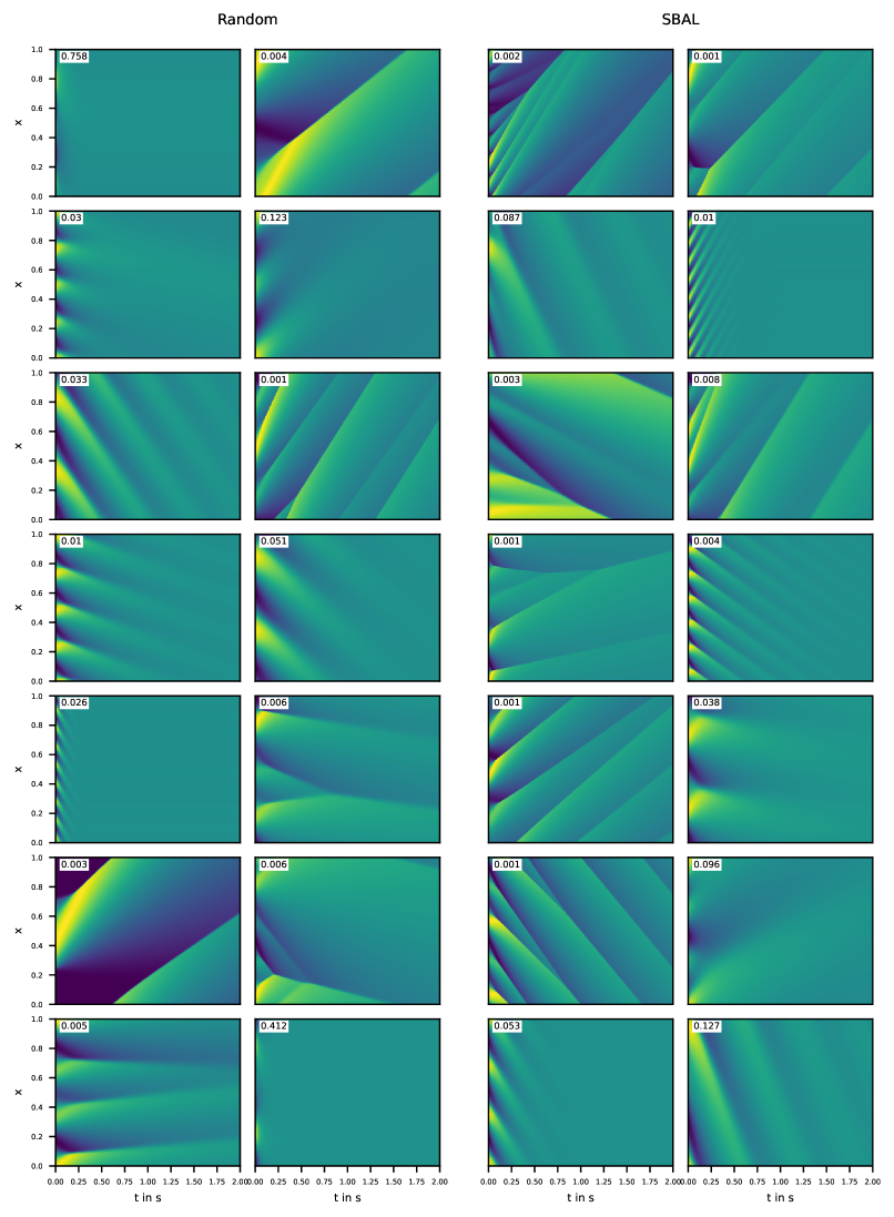
Figure 12: Example ground truth trajectories of random and SBAL on Burgers. The number on the top left of the trajectories shows the PDE parameter $\nu$.

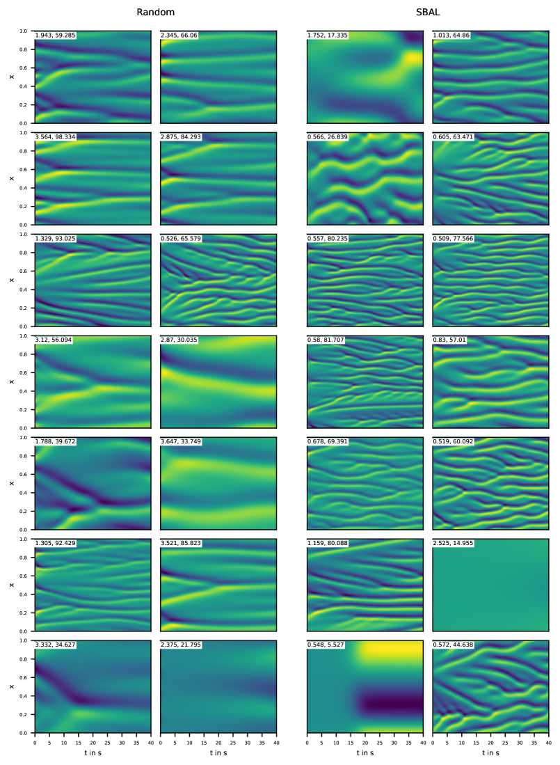
Figure 13: Example ground truth trajectories of random and SBAL on KS. The number on the top left of the trajectories shows the parameters ($\nu$, L). The x-axis is shown in normalized values between 0 and 1 independent of the variable domain length $L$.

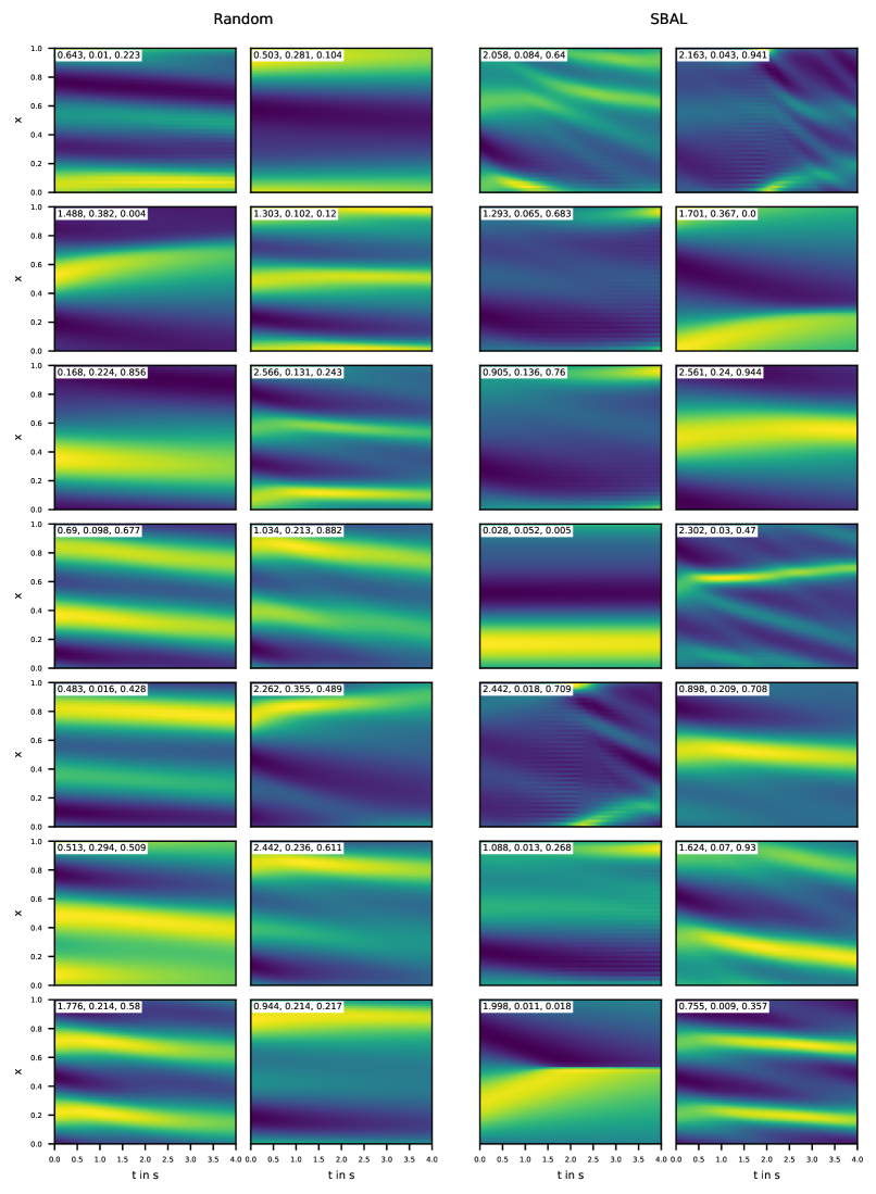
Figure 14: Example ground truth trajectories of random and SBAL on CE. The numbers on the top left of the trajectories shows the PDE parameters ($\alpha$, $\beta$, $\gamma$).

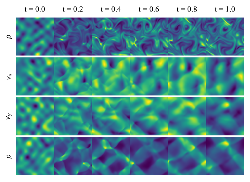
Figure 15: Example ground truth trajectory of CNS.

F.2 IC Parameter Marginal Distributions

Figures 16, 17, 18 and 19 show the marginal distributions of the random parameters of the IC generators, i.e. the random variables drawn which are then transformed using a deterministic function to the actual IC. For example, the KS IC generator draws amplitudes and phases from a uniform distribution and uses them afterward for the superposition of sine waves. If multiple numbers are drawn from each type of variable, we put them together, e.g., in the case of KS, multiple amplitudes are drawn for the different waves, but Fig. 17 only shows the distribution of all amplitude variables mixed. The distribution curves for continuous variables are computed using kernel density estimation. The shaded areas (vertical lines for discrete variables) show the standard deviation between the marginal distributions of different random seeds.

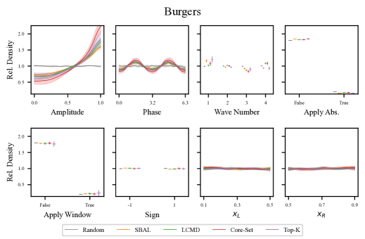
Figure 16: Marginal distribution of the parameters of the ICs sampled by the AL methods for Burgers. Displayed as the ratio to the density of the uniform distribution.

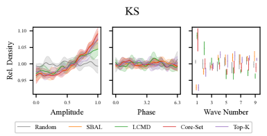
Figure 17: Marginal distribution of the parameters of the ICs sampled by the AL methods for KS. Displayed as the ratio to the density of the uniform distribution.

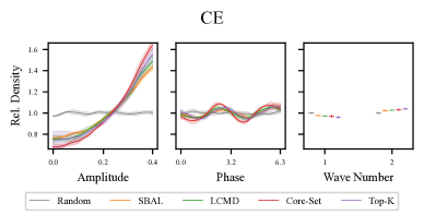
Figure 18: Marginal distribution of the parameters of the ICs sampled by the AL methods for CE. Displayed as the ratio to the density of the uniform distribution.

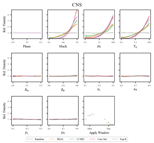
Figure 19: Marginal distribution of the parameters of the ICs sampled by the AL methods for 2D CNS. Displayed as the ratio to the density of the uniform distribution.

F.3 PDE Parameter Marginal Distributions

Similarly Fig. 20 shows the KDE estimates of the dataset after the final AL iteration for the PDE parameters.

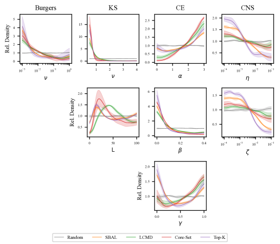
Figure 20: Marginal distribution of the PDE parameters, including the standard deviation between different runs. Displayed as the ratio to the density of the test distribution.

References

- Aikawa et al. (2023) Yuri Aikawa, Naonori Ueda, and Toshiyuki Tanaka. Improving the efficiency of training physics-informed neural networks using active learning. In The 37th Annual Conference of the Japanese Society for Artificial Intelligence, 2023.
- Arthurs & King (2021) Christopher J. Arthurs and Andrew P. King. Active training of physics-informed neural networks to aggregate and interpolate parametric solutions to the navier-stokes equations. J. Comput. Phys., 438:110364, 2021.
- Ash et al. (2021) Jordan Ash, Surbhi Goel, Akshay Krishnamurthy, and Sham Kakade. Gone fishing: Neural active learning with fisher embeddings. Advances in Neural Information Processing Systems, 34:8927–8939, 2021.
- Ash et al. (2019) Jordan T Ash, Chicheng Zhang, Akshay Krishnamurthy, John Langford, and Alekh Agarwal. Deep batch active learning by diverse, uncertain gradient lower bounds. In International Conference on Learning Representations, 2019.
- Bajracharya et al. (2024) Pradeep Bajracharya, Javier Quetzalcóatl Toledo-Marín, Geoffrey Fox, Shantenu Jha, and Linwei Wang. Feasibility study on active learning of smart surrogates for scientific simulations. arXiv preprint arXiv:2407.07674, 2024.
- Brandstetter et al. (2021) Johannes Brandstetter, Daniel E Worrall, and Max Welling. Message passing neural pde solvers. In International Conference on Learning Representations, 2021.
- Brandstetter et al. (2022) Johannes Brandstetter, Max Welling, and Daniel E Worrall. Lie point symmetry data augmentation for neural pde solvers. In International Conference on Machine Learning, pp. 2241–2256. PMLR, 2022.
- Brandstetter et al. (2023) Johannes Brandstetter, Rianne van den Berg, Max Welling, and Jayesh K. Gupta. Clifford neural layers for PDE modeling. In The Eleventh International Conference on Learning Representations, ICLR 2023, Kigali, Rwanda, May 1-5, 2023, 2023.
- Burark et al. (2023) Priyanshu Burark, Karn Tiwari, Meer Mehran Rashid, Prathosh A P, and N. M. Anoop Krishnan. Codbench: A critical evaluation of data-driven models for continuous dynamical systems. CoRR, abs/2310.01650, 2023.
- Cho et al. (2024) Woojin Cho, Minju Jo, Haksoo Lim, Kookjin Lee, Dongeun Lee, Sanghyun Hong, and Noseong Park. Parameterized physics-informed neural networks for parameterized PDEs. In Proceedings of the 41st International Conference on Machine Learning, volume 235 of Proceedings of Machine Learning Research, pp. 8510–8533. PMLR, 21–27 Jul 2024.
- Dresdner et al. (2023) Gideon Dresdner, Dmitrii Kochkov, Peter Christian Norgaard, Leonardo Zepeda-Nunez, Jamie Smith, Michael Brenner, and Stephan Hoyer. Learning to correct spectral methods for simulating turbulent flows. Transactions on Machine Learning Research, 2023.
- Gao & Wang (2023) Wenhan Gao and Chunmei Wang. Active learning based sampling for high-dimensional nonlinear partial differential equations. Journal of Computational Physics, 475:111848, 2023.
- Geifman & El-Yaniv (2017) Yonatan Geifman and Ran El-Yaniv. Deep active learning over the long tail. arXiv preprint arXiv:1711.00941, 2017.
- Gupta & Brandstetter (2023) Jayesh K Gupta and Johannes Brandstetter. Towards multi-spatiotemporal-scale generalized pde modeling. Transactions on Machine Learning Research, 2023.
- Hagnberger et al. (2024) Jan Hagnberger, Marimuthu Kalimuthu, Daniel Musekamp, and Mathias Niepert. Vectorized conditional neural fields: A framework for solving time-dependent parametric partial differential equations. In Proceedings of the 41st International Conference on Machine Learning, volume 235 of Proceedings of Machine Learning Research, pp. 17189–17223. PMLR, 21–27 Jul 2024.
- Hao et al. (2023) Zhongkai Hao, Jiachen Yao, Chang Su, Hang Su, Ziao Wang, Fanzhi Lu, Zeyu Xia, Yichi Zhang, Songming Liu, Lu Lu, and Jun Zhu. PINNacle: A comprehensive benchmark of physics-informed neural networks for solving pdes. CoRR, abs/2306.08827, 2023.
- Hassan et al. (2023) Sheikh Md Shakeel Hassan, Arthur Feeney, Akash Dhruv, Jihoon Kim, Youngjoon Suh, Jaiyoung Ryu, Yoonjin Won, and Aparna Chandramowlishwaran. Bubbleml: A multiphase multiphysics dataset and benchmarks for machine learning. In Advances in Neural Information Processing Systems, 2023.
- Hendrycks & Gimpel (2016) Dan Hendrycks and Kevin Gimpel. Gaussian error linear units (gelus). arXiv preprint arXiv:1606.08415, 2016.
- Holzmüller et al. (2023) David Holzmüller, Viktor Zaverkin, Johannes Kästner, and Ingo Steinwart. A framework and benchmark for deep batch active learning for regression. J. Mach. Learn. Res., 24:164:1–164:81, 2023.
- Hyman & Nicolaenko (1986) James M Hyman and Basil Nicolaenko. The kuramoto-sivashinsky equation: a bridge between pde’s and dynamical systems. Physica D: Nonlinear Phenomena, 18(1-3):113–126, 1986.
- Janny et al. (2023) Steeven Janny, Aurélien Béneteau, Madiha Nadri, Julie Digne, Nicolas Thome, and Christian Wolf. EAGLE: large-scale learning of turbulent fluid dynamics with mesh transformers. In The Eleventh International Conference on Learning Representations, ICLR 2023, Kigali, Rwanda, May 1-5, 2023, 2023.
- Kapoor et al. (2023) Taniya Kapoor, Abhishek Chandra, Daniel Tartakovsky, Hongrui Wang, Alfredo Núñez, and Rolf Dollevoet. Neural oscillators for generalizing parametric pdes. In The Symbiosis of Deep Learning and Differential Equations III, 2023.
- Kim et al. (2021) Yoon-Yeong Kim, Kyungwoo Song, JoonHo Jang, and Il-Chul Moon. LADA: Look-Ahead Data Acquisition via augmentation for deep active learning. Advances in Neural Information Processing Systems, 34:22919–22930, 2021.
- Kirsch (2023) Andreas Kirsch. Black-box batch active learning for regression. Transactions on Machine Learning Research, 2023.
- Kirsch et al. (2023) Andreas Kirsch, Sebastian Farquhar, Parmida Atighehchian, Andrew Jesson, Frédéric Branchaud-Charron, and Yarin Gal. Stochastic batch acquisition: A simple baseline for deep active learning. Transactions on Machine Learning Research, 2023.
- Lanthaler et al. (2023) Samuel Lanthaler, Roberto Molinaro, Patrik Hadorn, and Siddhartha Mishra. Nonlinear reconstruction for operator learning of pdes with discontinuities. In The Eleventh International Conference on Learning Representations, ICLR. OpenReview.net, 2023.
- Lanthaler et al. (2024) Samuel Lanthaler, Zongyi Li, and Andrew M. Stuart. Nonlocality and nonlinearity implies universality in operator learning. CoRR, 2024.
- Lewy et al. (1928) H Lewy, K Friedrichs, and R Courant. Über die partiellen differenzengleichungen der mathematischen physik. Mathematische annalen, 100:32–74, 1928.
- Li et al. (2020a) Shibo Li, Wei Xing, Robert Kirby, and Shandian Zhe. Multi-fidelity bayesian optimization via deep neural networks. Advances in Neural Information Processing Systems, 33:8521–8531, 2020a.
- Li et al. (2021) Shibo Li, Robert Kirby, and Shandian Zhe. Batch multi-fidelity bayesian optimization with deep auto-regressive networks. Advances in Neural Information Processing Systems, 34:25463–25475, 2021.
- Li et al. (2023) Shibo Li, Xin Yu, Wei Xing, Mike Kirby, Akil Narayan, and Shandian Zhe. Multi-resolution active learning of fourier neural operators. arXiv preprint arXiv:2309.16971, 2023.
- Li et al. (2020b) Zongyi Li, Nikola Kovachki, Kamyar Azizzadenesheli, Burigede Liu, Kaushik Bhattacharya, Andrew Stuart, and Anima Anandkumar. Fourier neural operator for parametric partial differential equations. arXiv preprint arXiv:2010.08895, 2020b.
- Lippe et al. (2023) Phillip Lippe, Bas Veeling, Paris Perdikaris, Richard E. Turner, and Johannes Brandstetter. Pde-refiner: Achieving accurate long rollouts with neural PDE solvers. In Advances in Neural Information Processing Systems, 2023.
- Liu et al. (2024) Tianlin Liu, Jose Antonio Lara Benitez, Amirehsan Khorashadizadeh, Florian Faucher, Maarten V de Hoop, and Ivan Dokmanić. Wavebench: Benchmarking data-driven solvers for linear wave propagation pdes. Transactions on Machine Learning Research Journal, 2024.
- Lookman et al. (2019) Turab Lookman, Prasanna V Balachandran, Dezhen Xue, and Ruihao Yuan. Active learning in materials science with emphasis on adaptive sampling using uncertainties for targeted design. npj Computational Materials, 5(1):21, 2019.
- Lu et al. (2019) Lu Lu, Pengzhan Jin, and George Em Karniadakis. Deeponet: Learning nonlinear operators for identifying differential equations based on the universal approximation theorem of operators. arXiv preprint arXiv:1910.03193, 2019.
- Luo et al. (2023) Yining Luo, Yingfa Chen, and Zhen Zhang. Cfdbench: A comprehensive benchmark for machine learning methods in fluid dynamics. CoRR, abs/2310.05963, 2023.
- Mao & Meng (2023) Zhiping Mao and Xuhui Meng. Physics-informed neural networks with residual/gradient-based adaptive sampling methods for solving partial differential equations with sharp solutions. Applied Mathematics and Mechanics, 44(7):1069–1084, 2023.
- Meduri et al. (2020) Venkata Vamsikrishna Meduri, Lucian Popa, Prithviraj Sen, and Mohamed Sarwat. A comprehensive benchmark framework for active learning methods in entity matching. In Proceedings of the 2020 ACM SIGMOD international conference on management of data, pp. 1133–1147, 2020.
- Mehrjou et al. (2021) Arash Mehrjou, Ashkan Soleymani, Andrew Jesson, Pascal Notin, Yarin Gal, Stefan Bauer, and Patrick Schwab. Genedisco: A benchmark for experimental design in drug discovery. In International Conference on Learning Representations, 2021.
- Mouli et al. (2024) S. Chandra Mouli, Danielle C. Maddix, Shima Alizadeh, Gaurav Gupta, Andrew Stuart, Michael W. Mahoney, and Yuyang Wang. Using uncertainty quantification to characterize and improve out-of-domain learning for pdes. In International Conference on Machine Learning, ICML, volume abs/2403.10642 of Proceedings of Machine Learning Research. PMLR, 2024.
- Moustapha et al. (2022) Maliki Moustapha, Stefano Marelli, and Bruno Sudret. Active learning for structural reliability: Survey, general framework and benchmark. Structural Safety, 96:102174, 2022.
- Ovadia et al. (2023) Oded Ovadia, Eli Turkel, Adar Kahana, and George Em Karniadakis. Ditto: Diffusion-inspired temporal transformer operator. CoRR, abs/2307.09072, 2023.
- Pestourie et al. (2020) Raphaël Pestourie, Youssef Mroueh, Thanh V Nguyen, et al. Active learning of deep surrogates for pdes: application to metasurface design. Computational Materials, 6(1):164, 2020.
- Pestourie et al. (2021) Raphaël Pestourie, Youssef Mroueh, Christopher Vincent Rackauckas, Payel Das, and Steven Glenn Johnson. Data-efficient training with physics-enhanced deep surrogates. In AAAI 2022 Workshop on AI for Design and Manufacturing (ADAM), 2021.
- Pestourie et al. (2023) Raphaël Pestourie, Youssef Mroueh, Chris Rackauckas, Payel Das, and Steven G. Johnson. Physics-enhanced deep surrogates for partial differential equations. Nat. Mac. Intell., 5(12):1458–1465, 2023.
- Pickering et al. (2022) Ethan Pickering, Stephen Guth, George Em Karniadakis, and Themistoklis P Sapsis. Discovering and forecasting extreme events via active learning in neural operators. Nature Computational Science, 2(12):823–833, 2022.
- Pinsler et al. (2019) Robert Pinsler, Jonathan Gordon, Eric Nalisnick, and José Miguel Hernández-Lobato. Bayesian batch active learning as sparse subset approximation. Advances in neural information processing systems, 32, 2019.
- Psaros et al. (2023) Apostolos F. Psaros, Xuhui Meng, Zongren Zou, Ling Guo, and George Em Karniadakis. Uncertainty quantification in scientific machine learning: Methods, metrics, and comparisons. J. Comput. Phys., 477:111902, 2023.
- Rahman et al. (2022) Md Ashiqur Rahman, Zachary E. Ross, and Kamyar Azizzadenesheli. U-NO: u-shaped neural operators. Transactions on Machine Learning Research, abs/2204.11127, 2022.
- Raissi et al. (2019) Maziar Raissi, Paris Perdikaris, and George E Karniadakis. Physics-informed neural networks: A deep learning framework for solving forward and inverse problems involving nonlinear partial differential equations. Journal of Computational physics, 378:686–707, 2019.
- Rauch et al. (2023) Lukas Rauch, Matthias Aßenmacher, Denis Huseljic, Moritz Wirth, Bernd Bischl, and Bernhard Sick. Activeglae: A benchmark for deep active learning with transformers. In Joint European Conference on Machine Learning and Knowledge Discovery in Databases, pp. 55–74. Springer, 2023.
- Ren et al. (2023) Simiao Ren, Yang Deng, Willie J. Padilla, Leslie M. Collins, and Jordan M. Malof. Deep active learning for scientific computing in the wild. CoRR, abs/2302.00098, 2023.
- Ronneberger et al. (2015) Olaf Ronneberger, Philipp Fischer, and Thomas Brox. U-net: Convolutional networks for biomedical image segmentation. In Medical image computing and computer-assisted intervention–MICCAI 2015: 18th international conference, pp. 234–241. Springer, 2015.
- Sahli Costabal et al. (2020) Francisco Sahli Costabal, Yibo Yang, Paris Perdikaris, Daniel E Hurtado, and Ellen Kuhl. Physics-informed neural networks for cardiac activation mapping. Frontiers in Physics, 8:42, 2020.
- Sener & Savarese (2018) Ozan Sener and Silvio Savarese. Active learning for convolutional neural networks: A core-set approach. In International Conference on Learning Representations, 2018.
- Seung et al. (1992) H Sebastian Seung, Manfred Opper, and Haim Sompolinsky. Query by committee. In Proceedings of the fifth annual workshop on Computational learning theory, pp. 287–294, 1992.
- Takamoto et al. (2022) Makoto Takamoto, Timothy Praditia, Raphael Leiteritz, Daniel MacKinlay, Francesco Alesiani, Dirk Pflüger, and Mathias Niepert. Pdebench: An extensive benchmark for scientific machine learning. In NeurIPS, 2022.
- Takamoto et al. (2023) Makoto Takamoto, Francesco Alesiani, and Mathias Niepert. Learning neural PDE solvers with parameter-guided channel attention. In International Conference on Machine Learning, ICML, volume 202 of Proceedings of Machine Learning Research, pp. 33448–33467. PMLR, 2023.
- Thakur (2023) Akshay Thakur. Uncertainty Quantification for Signal-to-Signal Regression-Based Neural Operator Frameworks. 7 2023.
- Toshev et al. (2023) Artur P. Toshev, Gianluca Galletti, Fabian Fritz, Stefan Adami, and Nikolaus A. Adams. Lagrangebench: A lagrangian fluid mechanics benchmarking suite. In Advances in Neural Information Processing Systems, 2023.
- Tsymbalov et al. (2018) Evgenii Tsymbalov, Maxim Panov, and Alexander Shapeev. Dropout-based active learning for regression. In Analysis of Images, Social Networks and Texts: 7th International Conference, AIST 2018, Moscow, Russia, July 5–7, 2018, Revised Selected Papers 7, pp. 247–258. Springer, 2018.
- Vaswani et al. (2017) Ashish Vaswani, Noam Shazeer, Niki Parmar, Jakob Uszkoreit, Llion Jones, Aidan N Gomez, Łukasz Kaiser, and Illia Polosukhin. Attention is all you need. Advances in neural information processing systems, 30, 2017.
- Wang et al. (2022) Alex Wang, Haotong Liang, Austin McDannald, Ichiro Takeuchi, and Aaron Gilad Kusne. Benchmarking active learning strategies for materials optimization and discovery. Oxford Open Materials Science, 2(1):itac006, 2022.
- Wang et al. (2023) Hong Wang, Zhongkai Hao, Jie Wang, Zijie Geng, Zhen Wang, Bin Li, and Feng Wu. Accelerating data generation for neural operators via krylov subspace recycling. In The Twelfth International Conference on Learning Representations, 2023.
- Weber et al. (2024) Tobias Weber, Emilia Magnani, Marvin Pförtner, and Philipp Hennig. Uncertainty quantification for fourier neural operators. In ICLR 2024 Workshop on AI4DifferentialEquations In Science, 2024.
- Wu et al. (2023a) Chenxi Wu, Min Zhu, Qinyang Tan, Yadhu Kartha, and Lu Lu. A comprehensive study of non-adaptive and residual-based adaptive sampling for physics-informed neural networks. Computer Methods in Applied Mechanics and Engineering, 403:115671, 2023a.
- Wu (2018) Dongrui Wu. Pool-based sequential active learning for regression. IEEE transactions on neural networks and learning systems, 30(5):1348–1359, 2018.
- Wu et al. (2023b) Dongxia Wu, Ruijia Niu, Matteo Chinazzi, Yian Ma, and Rose Yu. Disentangled multi-fidelity deep bayesian active learning. In International Conference on Machine Learning, pp. 37624–37634. PMLR, 2023b.
- Wu et al. (2023c) Dongxia Wu, Ruijia Niu, Matteo Chinazzi, Alessandro Vespignani, Yi-An Ma, and Rose Yu. Deep bayesian active learning for accelerating stochastic simulation. In Proceedings of the 29th ACM SIGKDD Conference on Knowledge Discovery and Data Mining, pp. 2559–2569, 2023c.
- Wu et al. (2024) Tailin Wu, Willie Neiswanger, Hongtao Zheng, Stefano Ermon, and Jure Leskovec. Uncertainty quantification for forward and inverse problems of pdes via latent global evolution. In Thirty-Eighth AAAI Conference on Artificial Intelligence, AAAI, pp. 320–328. AAAI Press, 2024.
- Wu & He (2018) Yuxin Wu and Kaiming He. Group normalization. In Proceedings of the European conference on computer vision (ECCV), pp. 3–19, 2018.
- Yang & Loog (2018) Yazhou Yang and Marco Loog. A benchmark and comparison of active learning for logistic regression. Pattern Recognition, 83:401–415, 2018.
- Zaverkin et al. (2022) Viktor Zaverkin, David Holzmüller, Ingo Steinwart, and Johannes Kästner. Exploring chemical and conformational spaces by batch mode deep active learning. Digital Discovery, 1:605–620, 2022.
- Zaverkin et al. (2024) Viktor Zaverkin, David Holzmüller, Henrik Christiansen, Federico Errica, Francesco Alesiani, Makoto Takamoto, Mathias Niepert, and Johannes Kästner. Uncertainty-biased molecular dynamics for learning uniformly accurate interatomic potentials. npj Computational Materials, 10(1):83, 2024.
- Zhan et al. (2021) Xueying Zhan, Huan Liu, Qing Li, and Antoni B Chan. A comparative survey: Benchmarking for pool-based active learning. In IJCAI, pp. 4679–4686, 2021.
- Zhang et al. (2024) Xuan Zhang, Jacob Helwig, Yuchao Lin, Yaochen Xie, Cong Fu, Stephan Wojtowytsch, and Shuiwang Ji. Sinenet: Learning temporal dynamics in time-dependent partial differential equations. CoRR, abs/2403.19507, 2024.
\startcontents[sections]