Gibbs Sampling gives Quantum Advantage at Constant Temperatures with $O(1)$-Local Hamiltonians

Abstract

Sampling from Gibbs states — states corresponding to system in thermal equilibrium — has recently been shown to be a task for which quantum computers are expected to achieve super-polynomial speed-up compared to classical computers, provided the locality of the Hamiltonian increases with the system size [BCL24]. We extend these results to show that this quantum advantage still occurs for Gibbs states of Hamiltonians with O(1)-local interactions at constant temperature by showing classical hardness-of-sampling and demonstrating such Gibbs states can be prepared efficiently using a quantum computer. In particular, we show hardness-of-sampling is maintained even for 5-local Hamiltonians on a 3D lattice. We additionally show that the hardness-of-sampling is robust when we are only able to make imperfect measurements. Beyond these hardness results, we present a lower bound on the temperatures that Gibbs states become easy to sample from classically in terms of the maximum degree of the Hamiltonian’s interaction graph.

1 Introduction

Gibbs states are fundamental objects of interest in many-body physics and chemistry, where they correspond to the state a system equilibrates to at a fixed temperature, and play an important role in semidefinite program solving and machine learning. One of the key uses cases for quantum computers has been to simulate many-body quantum systems, and with this in mind, a variety of quantum algorithms for Gibbs state preparation and sampling have been proposed, including a recent promising quantum generalisation of Metropolis-Hastings algorithm [CKG23, Gil+24].

At a given inverse temperature $\beta$ and Hamiltonian $H$, we define the Gibbs state as:

$$\rho(H,\beta)=\frac{e^{-\beta H}}{\operatorname{tr}\left[e^{-\beta H}\right]}.$$

Despite their importance, the computational complexity of calculating quantum Gibbs state properties, and whether there is a quantum advantage, has remained poorly understood — particularly at temperature independent of system size $\beta=\Theta(1)$. For Gibbs states of both classical and quantum Hamiltonians, efficient algorithms are known to exist above certain critical temperatures [Fra17, HMS20, MH21, YL23, RFA24, Bak+24], and at sufficiently low $O(1)$ temperatures Gibbs state properties of classical Hamiltonians are known to be NP-hard and even MA-complete to compute [Sly10, CBB10, SS12]. At even lower temperatures, $\beta=\Omega(\log(n))$, the Gibbs state has high overlap with the system’s ground state, and so for quantum Hamiltonians we can argue that cooling to these temperatures must be at least QMA-hard. For quantum Hamiltonians at $\beta=\Omega(\operatorname{poly}(n))$, computing expectation values of local observables measured on Gibbs states has been shown to be hard for a class QXC, “Quantum Approximate Counting” [Bra+22, Bra+24]. But exactly how this class relates to other classical and quantum complexity classes, and whether we expect similar hardness results for $\beta=\Theta(1)$, remains poorly understood. Gibbs sampling is also related to other important problems which have shown quantum speed-up including sampling log-concave distributions and volume estimation [Chi+22, Cha+23].

Recent work by [BCL24] consider the task of sampling bitstrings from quantum Gibbs states [BCL24]. That is, sampling from a distribution close in total variation distance to

$$P(x)=\frac{\bra{x}e^{-\beta H}\ket{x}}{\operatorname{tr}\left[e^{-\beta H}\right]},$$

for a bitstring $x\in\{0,1\}^{n}$. [BCL24] demonstrate that sampling bitstrings from families of Gibbs states of quantum Hamiltonians with $O(\log\log(n))$-local terms at temperature $\beta=\Theta(1)$ is classically intractable unless the polynomial hierarchy collapses to the third level [BCL24]. They further demonstrate that such Gibbs states can be prepared in polynomial time using a quantum computer, and hence the task of Gibbs sampling can be done efficiently with the aid of a quantum computer. Not only does this demonstrate a quantum advantage in Gibbs state preparation over classical computers — and thus may be a good test of so-called quantum supremacy — but it is arguably the first convincing demonstration that Gibbs states retain non-trivial quantum computational properties at $\beta=\Theta(1)$ temperatures.

In this work we build upon the work in [BCL24] and demonstrate there exist families of 5-local and 6-local Hamiltonians such that sampling from Gibbs states at $\beta=\Theta(1)$ temperatures remains classically intractable unless the polynomial hierarchy collapses to the third level.

Theorem 1 ((Informal) Classically Intractable Gibbs Sampling).

There exist two families $\mathcal{F}_{1},\mathcal{F}_{2}$ of efficiently constructable Hamiltonians such that sampling from a probability distribution $Q(x)$ satisfying:

$$\left\lVert Q(x)-\frac{\bra{x}e^{-\beta H}\ket{x}}{\operatorname{tr}\left[e^{-\beta H}\right]}\right\rVert_{1}\leq\epsilon,$$

is not possible for randomised classical algorithms unless the polynomial hierarchy collapses, for the following parameter regimes:

1. the Hamiltonians are 5-local, nearest-neighbour Hamiltonians on a 3D cubic lattice, where each qubit is involved in at most $4$ Hamiltonian terms, and $\epsilon=O(\exp(-n))$. Furthermore, we allow each single-qubit measurement outcome to be incorrect with an $O(1)$ probability.

2. the Hamiltonians are 6-local, and $\epsilon=O(1)$.

Sampling from a $Q(x)$ close to either of these distributions can be done efficiently using a quantum computer.

We prove our results by combining results from the hardness of sampling IQP circuits with results from measurement-based quantum computation and error-detection protocols. In particular, we utilise work on the hardness of sampling from IQP circuits developed by [FT16] [FT16] and [BMS17] [BMS17] to construct families of Hamiltonians whose corresponding Gibbs states inherent this hardness of sampling. We anticipate that the families of Hamiltonians in $\mathcal{F}_{1},\mathcal{F}_{2}$ are easier to realise experimentally than those presented in previous works.

Beyond showing hardness of Gibbs sampling for Hamiltonians with more restrictive physical properties, we seek to put bounds on the temperature regions where “dequantization” algorithms such those in [Bak+24] can effectively sample from Gibbs states. We find that our hardness results asymptotically complement easiness results from [Bak+24], but with a small gap in parameter scaling. In particular, we construct $6$-local Hamiltonians with max degree $\Delta$, for which sampling is classically intractable for inverse temperatures $\beta=\Omega(1/\sqrt{\Delta})$. We compare this to [Bak+24] [Bak+24, Theorem 1.6] who show that one can efficiently sample from Gibbs states for $O(1)$-local Hamiltonians at inverse temperatures $\beta=O\left(\frac{1}{\Delta}\right)$ using a polynomial-time classical algorithm.

We show how our results compare to existing work on the complexity of sampling from Gibbs States in Table 1.

	Hardness, [BCL24]	Easiness, [Bak+24]	Hardness, Sec. 3.2	Hardness, Sec. 3.3
Locality ($\ell$)	$O(\log\log(n))$	$O(1)$	$5$	$6$
Max. Degree ($\Delta$)	$O(\log(n))$	$O(1)$	$5$	$O(\log(n))$
Interaction Geometry	None	Any	3D Cubic Lattice	None
Sampling Precision ($\epsilon$)	$1/\operatorname{poly}(n)$	$1/\exp(n)$	$1/\exp(n)$	$1/\operatorname{poly}(n)$

Table 1: Comparison of results about the complexity of sampling Gibbs states at constant temperature. Here the “Easiness” result of [Bak+24] gives efficient algorithms for Gibbs sampling. The maximum degree refers to the number of Hamiltonian terms that each qubit is involved in. The “Interaction Geometry” row denotes which geometries the hardness/easiness results hold for. We also remark that the hardness of sampling shown in Sec. 3.2 has the added bonus of being robust to measurement error on the output bits

Paper Outline

In Section 2 we give the preliminaries and notation. Section 3 contains an overview of the proof techniques, as well as our main results: Section 3.2 proves hardness of sampling Gibbs states of 5-local Hamiltonians on a 3D lattice and Section 3.3 proves hardness for 6-local Hamiltonians. In Section 4, we show how these hardness results can be made robust to errors in measurement. In Section 5 we show that by increasing the maximum degree of Hamiltonians (i.e. the maximum number of terms which act on a single particle), we can increase the temperatures for which sampling remains classically hard. In Section 6 we suggest a heuristic method of demonstrating that we have prepared the desired Gibbs state. Finally, we discuss this work and open questions in Section 7.

2 Preliminaries

2.1 Notation

Consider a set of $n$ particles, each with local Hilbert space $\mathbb{C}^{d}$, then the full Hilbert space is $(\mathbb{C}^{d})^{\otimes n}$. For a Hilbert space $\mathcal{H}$ we denote the set of bounded linear operators as $\mathcal{B}(\mathcal{H})$. A Hamiltonian acting on $n$ qudits is a Hermitian operator $H\in\mathcal{B}((\mathbb{C}^{d})^{\otimes n})$. For the rest of this work will we consider the case $d=2$, i.e. the Hamiltonian acts on qubits. $\left\lVert\cdot\right\rVert$ will denote the operator norm, $\left\lVert\cdot\right\rVert_{1}$ will denote the Schatten 1-norm when acting on operators, and if acting on probability distributions is the standard $L1$ distance between probability distributions.

Hamiltonian Parameters.

The Hamiltonian is called a $k$-local Hamiltonian if we can write it as:

$$H=\sum_{i}h_{i}$$

if each $h_{i}$ acts on at most $k$ many qubits. Given a local Hamiltonian, we can define a interaction (hyper)graph, where the vertices are given by the qubits and the (hyper)edges are given by the qubits $h_{i}$ acts non-trivially on. We denote the maximum degree of the interaction graph as $\Delta$. We assume that $\left\lVert h_{i}\right\rVert=O(1)$ for all local terms in the Hamiltonian.

Thermal Physics.

Given a temperature $T\in\mathbb{R}^{+}$, we will work with the inverse temperature $\beta=1/T$. For a given Hamiltonian $H$ with eigenvalues $\{\lambda_{i}\}_{i}$, and a given inverse temperature $\beta$, the partition function is define as:

$$Z=\text{tr}\left[e^{-\beta H}\right]=\sum_{i}e^{-\beta\lambda_{i}},$$

and the associated Gibbs state is:

$$\rho(H,\beta)=\frac{1}{Z}e^{-\beta H}.$$

Noisy Circuits.

We will often discuss circuits by directly referring to their unitary matrix $C$, with the convention that $C\ket{0}^{\otimes n}$ is the output state after applying $C$ on $\ket{0}^{\otimes n}$. We will be interested in bit-flip noise in our circuit, and define the single-qubit channel:

$$\mathcal{D}_{p}(\rho)=(1-p)\rho+pX\rho X$$

We use the following notation to refer to the output distribution of a circuit with noise on the input state:

Definition 2 (Circuit Sampling Distributions).

For any circuit $C$ we will use $P_{C}$ to denote the output distribution of sampled bitstrings from $C$,

$$P_{C}(x)=|\bra{x}C\ket{0^{n}}|^{2},$$

and $P_{C,q}$ to denote the output distribution of sampled bitstrings from $C$ with independent single-qubit bit-flips applied on every input qubit with probability $q$:

$$P_{C,q}(x)=\operatorname{tr}\left[\ket{x}\bra{x}\cdot C(\mathcal{D}^{\otimes n}_{q}(\ket{0}\bra{0}^{\otimes n}))C^{\dagger}\right].$$

2.2 Parent Hamiltonian Construction for Quantum Circuits

Initially consider a non-interacting Hamiltonian on $n$ qubits:

$$H_{\text{NI}}=\sum_{i=1}^{n}\frac{1}{2}(\mathds{1}-Z_{i}).$$

It can be seen that the eigenstates of this Hamiltonian correspond to bitstrings $\ket{x}$ for $x\in\{0,1\}^{n}$, where the energy of eigenstate $\ket{x}$ is $\lambda_{x}=\operatorname{HW}(x)$, where $\operatorname{HW}$ denotes the Hamming weight of a string $x$. The zero-energy ground state is $\ket{0}^{\otimes n}$. The corresponding Gibbs state of the Hamiltonian is:

$$\frac{1}{Z}e^{-\beta H}=\frac{1}{Z}e^{-\beta\sum_{x\in\{0,1\}^{n}}\lambda_{x}\ket{x}\bra{x}}$$

and $Z=\sum_{x\in\{0,1\}^{n}}e^{-\beta\lambda_{x}}$. We see that $Z$ is the partition function for $n$ non-interacting spins, and hence $Z=(1+e^{-\beta})^{n}$. Now, given a circuit $C$ on $n$ qubits, we can define a parent Hamiltonian:

$$H_{C}=CH_{\text{NI}}C^{\dagger}.$$

2.3 Gibbs States of Parent Hamiltonians

We use the following two lemmas in our work. The first (implicitly used in [BCL24]) shows that for the set of parent Hamiltonians formed using quantum circuits, their Gibbs states are equivalent to the circuit with bit-flip noise acting on the input. Here the input noise strength is related to the temperature of the Gibbs state. We provide an explicit proof in Appendix B for completeness. Here the temperature of the Gibbs state corresponds to the strength of the bit-flip noise.

Lemma 3.

For any circuit $C$ constructed from $k$-local gates of depth $d$, there exists a $O(kd)$-local parent Hamiltonian $H_{C}$, such that:

$$\frac{1}{Z}e^{-\beta H_{C}} =C(\mathcal{D}_{q}^{\otimes n}(\ket{0}\bra{0}))C^{\dagger}$$

for $q=\frac{e^{-\beta}}{1+e^{-\beta}}$.

The second lemma, which is a large portion of the technical work in [BCL24], shows that a quantum computer can efficiently prepare the Gibbs States of these parent Hamiltonians.

Lemma 4 (Efficient Gibbs State Preparation for Parent Hamiltonians, Lemma 1.2 of [BCL24]).

Fix $\beta>0$, and let $H_{C}$ be the parent Hamiltonian of a quantum circuit $C$ on $n$ qubits, of depth $d$ and locality $\ell$. Then, there exists a quantum algorithm which can prepare the Gibbs state of $H$ at inverse-temperature $\beta$ up to an error $\epsilon$ in trace distance in time $O(2^{4\ell}2^{d}e^{\beta}n\operatorname{poly}(\log\frac{n}{\epsilon},\ell,\beta))$.

3 Hardness of Sampling Gibbs States with O(1)-Local Hamiltonians

3.1 Overview of Techniques

We wish to prove hardness of classically sampling the from Gibbs states of a Hamiltonian. To do so, we turn to Lemma 3: our goal is to find a family of circuits $C$ with corresponding parent Hamiltonians whose Gibbs states are hard to sample from with a classical computer but efficiently sampleable with a quantum computer. $C$ must satisfy the following requirements,

1. For some noise strength $q=O(1)$, $P_{C,q}$ must be hard to sample from with either inverse exponential or additive error.

2. $H_{C}$ must be $O(1)$-local.

3. $C$ must have $O(\log n)$ depth.

In this work, we will choose $C$ to be from the family of IQP circuits with the aim of maintaining classical hardness-of-sampling while ensuring the associated parent Hamiltonian remains $O(1)$-local. The main reason for choosing these circuits is that there are known constant depth IQP circuits which are hard to sample from Refs. [FT16, Han+18], and the shallowness of the circuit is useful to obtain $O(1)$-locality of the parent Hamiltonian. In particular, we need to choose a family of IQP circuits whose hardness of sampling is robust to bit-flip noise on the input. This is non-trivial since in many cases the presence of noise may make the IQP circuit classically easy to sample [BMS16, RWL24].

To prove our results, we use two separate error mitigation techniques. First, we use a result from [FT16] [FT16]. [FT16] make use of topologically protected circuits to ensure that, provided the circuit noise is below a certain threshold, exact sampling from the circuit remains difficult. Modifying this proof allows us to obtain hardness of sampling with inverse exponential error, and this allows us to arrive at $\mathcal{F}_{1}$ of Theorem 1, a family of $5$-local Hamiltonians with degree $5$, which are hard to sample from with inverse exponential error.

Second, we implement an error-detection strategy inspired by the techniques of Refs. [BMS17, BCL24], where parts of the circuit are repeated and we simultaneously introduce flag qubits which flip to show where an error may have occurred. This allows us to arrive at hardness of sampling from with additive error for $\mathcal{F}_{2}$, a family of Hamiltonians with $O(1)$ locality. Our hardness-of-sampling proof follows the similar outline as Ref. [BCL24], but here we prove hardness for different sets of circuits which allows us to obtain hardness for families of Hamiltonians with $O(1)$-locality rather than $O(\log\log(n))$-locality. We also note similar work on thermal states of measurement-based thermal states in [Fuj15].

Finally, by combining these two techniques, we obtain a family of $6$-local Hamiltonians with max degree $\Delta$, such that their Gibbs states are hard to sample from with inverse exponential error when $\beta=O(1/\sqrt{\Delta})$, which complements easiness results from [Bak+24].

3.2 Hardness of Sampling Gibbs States on 3D Lattices

[FT16] demonstrate a family of constant-depth, geometrically local IQP circuits which are hard to exactly sample from in the presence of noise of constant strength [FT16]. At a high level, [FT16] give a protocol in which a cluster state is constructed using a depth 4 IQP circuit. If the noise level is sufficiently smaller than the threshold value for topologically protected MBQC, then the output distribution of the circuit cannot be exactly sampled from. Provided the noise is restricted to bit-flip noise and kept below a threshold strength of $\sim 0.134$, then T-gate synthesis is still possible in the circuit, and postselecting on error-free outcomes allows one to decide PostBQP-complete problems. Since $\textsf{PostBQP}=\textsf{PP}$ and it is believed that $\textsf{PostBQP}\not\subseteq\textsf{PostBPP}$ unless the polynomial hierarchy collapses to the third level, then sampling from the noisy circuit is still hard [Aar05].

By taking this set of topologically protect circuits from [FT16] we prove the following lemma in Appendix A.

Lemma 5.

There exists a family of IQP circuits $\mathcal{C}$, constructed on a 3D cubic lattice, consisting of a single layer of $e^{iZ\pi/8}$ gates and 4 layers of nearest-neighbour $e^{iZZ\pi/4}$ gates, such that sampling from any probability distribution $Q$ over bitstrings which satisfies $\|P_{C,q}-Q\|_{1}<(1-q)^{n}2^{-6n-4}/5$ is not possible with a classical polynomial algorithm, unless the polynomial hierarchy collapses to the third level, when $q<0.134$.

We now want to use this family of classically hard-to-sample circuits to generate hard-to-sample Gibbs states. In particular, we combine this hard-to-sample from family of IQP circuits with the fact that the Gibbs states of IQP parent Hamiltonians look like the output of noisy IQP circuits, as per Lemma 3, and we get the following.

Theorem 6 (Classical Hardness of Gibbs Sampling).

One can efficiently construct a family of $5$-local Hamiltonians on a 3D cubic lattice of qubits, $\{H_{C}\}_{C}$, whose Gibbs states at $\beta=O(1)$ are hard to classically sample from with $1$-error $(1-q)^{n}2^{-6n-4}/5$, unless the polynomial hierarchy collapses to the 3rd level.

Proof.

We choose a hard-to-sample IQP circuit $C$ from Lemma 5 and specify the new Hamiltonian as $H_{C}=CH_{\text{NI}}C^{\dagger}$. By Lemma 3, the output distribution of the Gibbs states of $H_{C}$ is exactly $P_{C,q}$ Choosing:

$$q=\frac{e^{-\beta}}{1+e^{-\beta}}\leq 0.134$$ (1)

and we see that the output distribution must be hard to sample from, as per Lemma 5. Thus we see that for $\beta\gtrsim 1.87=O(1)$, it is hard to sample this distribution.

To see that the locality of $H_{C}$ is $5$, we note that for each qubit $i$, there are at most $4$ gates acting on qubit $i$ in $C$, each of which introduces interaction with at most $4$ other qubits. Thus, when conjugating the $Z_{i}$ term of $H_{NI}$ with the gates of $C$, it becomes an at most $5$-local term. ∎

Notably, in order to prove hardness of sampling with inverse exponential error from a noisy IQP circuit, a postselection argument suffices, rather than a full fault-tolerant encoding. Thus, there is no added overhead needed to give hardness of sampling, which ensures that the locality of the parent Hamiltonian is purely determined by the logical IQP circuit structure, which has low depth and locality. This is not true for the circuits and parent Hamiltonians in the next section, or in Ref. [BCL24] where additional elements need to be added to the circuit to allow for error detection.

3.3 Hardness of Gibbs Sampling to O(1/poly(N)) Error

While the hardness of sampling from noiseless IQP circuits with inverse exponential error can be obtained through a postselection argument, proving hardness of sampling with additive error typically requires a few more ingredients (e.g. anticoncentration, average-to-worst case reduction). Here, we use existing results from [Han+18] [Han+18] which construct a family of constant-depth IQP circuits that exhibit such hardness (up to some complexity-theoretic conjectures).

Lemma 7.

(Corollary 12 of [Han+18]) There exists a family of constant depth IQP circuits $\{C_{n}\}_{n}\geq 1$ on a 2D square lattice of $n$ qubits, such that no randomised classical polynomial-time algorithm can sample from the output distribution of $C_{n}$ up to additive $1$ error of $\delta=1/192$, assuming the average-case hardness of computing a fixed family of partition functions, and the non-collapse of the polynomial hierarchy.

Now we would like to show that the hardness of sampling from this circuit is robust to input noise, and without postselection (as this would make it more difficult to show hardness of additive error sampling). This task has been explored in Refs. [BMS17, BCL24] for IQP circuits, and they each provide a method of encoding an arbitrary IQP circuit into a larger, noise-robust circuit. Here, we describe an encoding method that is heavily inspired by these techniques.

Our construction is as follows. Suppose the initial circuit acts on $n$ qubits. Fix some positive integer $r$. For each ‘logical’ qubit $i$ in the circuit of Lemma 7 (initialised in the $\ket{0}$ state), initialise a block of $r$ ‘physical’ qubits in the $\ket{0}$ state, and label them $i_{1},\ldots,i_{r}$. For each block $i$, apply $r-1$ CNOT gates which are all controlled on $i_{1}$, and targeting a qubit in $i_{2},\ldots,i_{r}$. Let the unitary corresponding to this CNOT network be $B$. Then, apply the logical circuit (from Lemma 7) amongst the first qubits of each block (qubits labelled $1_{1},2_{1},\ldots,n_{1}$). Finally, measure all qubits in the computational basis. See Fig. 1 for an example of such a circuit with $r=2$.

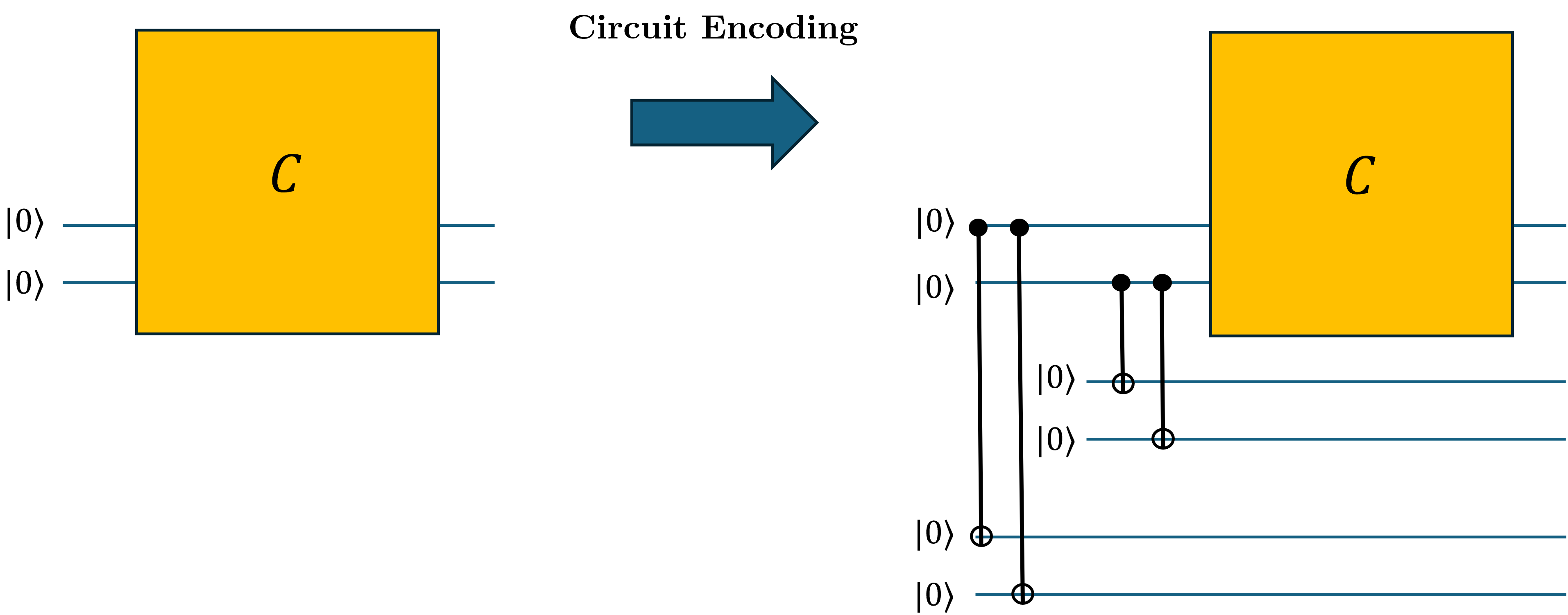
Figure 1: The encoding of the IQP circuit $C$ with $r=3$. For clarity, only two input qubits are shown explicitly, but the procedure applies to all qubits present.

We see that if the initial logical qubit is flipped by noise at the start of the circuit, the CNOT network associated with that qubit should flip all the associated ancillary qubits to the $\ket{1}$ state, thus flagging the error which can be corrected in postprocessing. We require $r$ auxiliary qubits to flag the error as the auxiliary qubits themselves may have noise incident on them, and so the multiple copies acts a repetition code to suppress this case.

We show in Appendix C that with classical post-processing, one can recover the logical output distribution with an error rate that is exponentially suppressed in $r$. Crucially, we only require $r=O(1)$ which means the parent Hamiltonian remains $O(1)$-local. Our proof works by examining the propagation of Pauli’s through the CNOT network.

Lemma 8.

Let $C$ be an arbitrary IQP circuit constructed with $2$-qubit gates of depth $d$ on $n$ qubits. Then, for any integer parameter $r\geq 1$, there is an encoded IQP circuit $C^{*}$ constructed with $2$-qubit gates of depth $d+r$ on $nr$ qubits, and a decoding algorithm $A^{*}$ such that,

$$A^{*}(P_{C^{*},q})=P_{C,p_{\text{fail}}}$$ (2)

where $p_{\text{fail}}\leq(4q(1-q))^{r/2}$. Furthermore, the parent Hamiltonian of $C^{*}$ has locality $k\leq d+2$ and degree $\Delta\leq r(d+1)$

Thus, given an initial circuit $C$, obtain a new circuit composed of an initial set of CNOT layers, followed by an IQP circuit. The output of the error-free circuit can be extracted from classical post-processing. We can put this all together to obtain the following theorem.

Theorem 9.

One can efficiently construct a family of $6$-local Hamiltonians, $\{H_{C}\}_{C}$, whose Gibbs states at $\beta=O(1)$ are hard to classically sample from with constant $1$-error up to $1/192$, unless the polynomial hierarchy collapses to the 3rd level.

Proof.

We choose a hard-to-sample IQP circuit $C$ from Lemma 7. Then, we encode $C$ into $C^{*}$ as in Lemma 8 (with parameter $r$ to be set later), and specify the new Hamiltonian as $H_{C^{*}}=C^{*}H_{\text{NI}}C^{*\dagger}$. By Lemma 3, the output distribution of the Gibbs states of $H_{C^{*}}$ at constant temperature is exactly $P_{C^{*},q}$. Using $A^{*}$, we can postprocess this to obtain $P_{C,p_{\text{fail}}}$ where $p_{\text{fail}}\leq(4q(1-q))^{r/2}$. Therefore, it suffices to choose $r=O(\log n)$ in order to set the probability of an error happening on any qubit to be $O(1/n)$. By increasing $r$, we can set the approximation error arbitrarily lower than $1/192$. Thus, it is hard to sample from the Gibbs states of $H_{C^{*}}$ with constant $1$ error up to $\delta=1/192$. ∎

Additionally, in Appendix C we show that the output distributions of this work and previous noise-robust IQP encodings (specifically those presented in here and in Refs. [BMS17, BCL24]) are equivalent, up to reversible classical postprocessing. This highlights the fact that improvements in Hamiltonian locality have not been obtained by considering very different output distributions, but rather, different Hamiltonian constructions.

3.4 Quantum Advantage from Gibbs Sampling of O(1)-Local Hamiltonians

So far we have proven hardness of sampling from Gibbs states for the families of parent Hamiltonians in Section 3.2 and Section 3.3. Here we employ the Gibbs state preparation algorithm of Ref. [Che+23] in conjunction with Lemma 4.

Theorem 10 (Quantum Advantage with $O(1)$-Local Hamiltonians).

The Gibbs states associated with the families of parent Hamiltonians in Theorem 6 and Theorem 9 can be sampled from efficiently using a quantum computer in the same parameter regimes for which they are classically hard.

Proof.

For both of the families of Hamiltonians in Theorem 6 and Theorem 9 the Hamiltonians are $O(1)$-local, hence the runtime of the Gibbs state preparation algorithm in Lemma 4 with $\beta=\Theta(1)$, $\ell=O(1)$ and $\epsilon=\frac{1}{9}(1+e^{-\beta})^{-n}2^{-6n-4}$ gives a total runtime of $O(2^{4\ell}2^{d}e^{\beta}n\operatorname{poly}(\log\frac{n}{\epsilon},\ell,\beta))=O(\operatorname{poly}(n))$. Thus sampling from these distributions can be done in polynomial time for a quantum computer.

On the other hand, as shown in Theorem 6 and Theorem 9, sampling from these Gibbs states in this parameter regime is classically intractable unless the polynomial hierarchy collapses to the third level. ∎

4 Measurement Errors in Gibbs State Sampling

When trying to show a quantum advantage in Gibbs state sampling, there are two sources of error: (a) we can only approximately prepare the true Gibbs state, and (b) when sampling, we expect our measurements to have an error associated with them. Here we show that, even with these two sources of error, we are sampling from a probability distribution that we do not expect to be able to sample from classically.

Theorem 11.

Consider a family of IQP circuits $\mathcal{C}$, the associated parent Hamiltonians $\{H_{C}\}_{C\in\mathcal{C}}$ and an inverse temperature $\beta=\Theta(1)$. There are a family of efficiently preparable states $\{\tilde{\rho}_{C}\}_{C\in\mathcal{C}}$ in time $\operatorname{poly}(n)$ on a quantum computer, such that for $\epsilon=\frac{1}{9}(1+e^{-\beta})^{-n}2^{-6n-4}$,

$$\left\lVert\tilde{\rho}_{C}-\rho(H_{C},\beta)\right\rVert_{1}\leq\epsilon$$

and sampling from $\mathcal{D}_{q}^{\otimes n}(\tilde{\rho}_{C})$ (i.e. with imperfect measurements with single qubit measurement error $q=\Theta(1)$) is not possible using a randomised classical algorithm unless the polynomial hierarchy collapses to the 3rd level.

Proof.

From Lemma 4, we see that preparing $\tilde{\rho}_{C}$ to this precision is possible in $O(\operatorname{poly}(n))$ time using a quantum computer. The distribution we are sampling corresponding to faulty measurements with probability $q$ on the prepared state $\tilde{\rho}$ approximating $\rho(H_{C},\beta)$ is:

$$\tilde{P}(x)=\operatorname{tr}\left[\ket{x}\bra{x}\cdot\mathcal{D}_{q}^{\otimes n}(\tilde{\rho}_{C})\right].$$

We using Hölder’s inequality:

$$\left\lVert\tilde{P}(x)-\operatorname{tr}\left[\ket{x}\bra{x}\mathcal{D}_{q}^{\otimes n}(\rho(H_{C},\beta))\right]\right\rVert_{1} \leq\left\lVert\mathcal{D}_{q}^{\otimes n}(\tilde{\rho}_{C})-\mathcal{D}_{q}^{\otimes n}(\rho(H_{C},\beta))\right\rVert_{1}.$$

Since $\left\lVert\tilde{\rho}_{C}-\rho(H_{C},\beta)\right\rVert_{1}\leq\epsilon$, then we see:

$$\left\lVert\mathcal{D}_{q}^{\otimes n}(\tilde{\rho}_{C}-\rho(H_{C},\beta))\right\rVert_{1} \leq\left\lVert\tilde{\rho}_{C}-\rho(H_{C},\beta)\right\rVert_{1}$$

$$\leq\epsilon,$$

where we have used that $\mathcal{D}^{\otimes n}(\cdot)$ is a CPTP map. Thus we see that sampling from $\tilde{P}(x)$ approximates sampling from the Gibbs state $\mathcal{D}^{\otimes n}(\rho(H_{C},\beta))$ with imperfect measurements.

Now, we show that $\mathcal{D}^{\otimes n}(\rho(H_{C},\beta))$ is also hard to classically sample from. We know from Lemma 3 that we can write Gibbs states of parent Hamiltonians as equivalent to the output of a noisy IQP circuit:

$$\mathcal{D}^{\otimes n}_{q}\left(\frac{e^{-\beta H_{C}}}{Z}\right) =\mathcal{D}^{\otimes n}_{q}\mathcal{D}^{\otimes n}_{\frac{e^{-\beta}}{1+e^{-\beta}}}(C\ket{0}\bra{0}^{\otimes n}C^{\dagger})$$

$$=\mathcal{D}^{\otimes n}_{q^{\prime}}(C\ket{0}\bra{0}^{\otimes n}C^{\dagger})$$

$$=\frac{e^{-\beta^{\prime}H_{C}}}{Z}$$

where we have defined $q^{\prime}=(\frac{e^{-\beta}}{1+e^{-\beta}})(1-q)+q(1-\frac{e^{-\beta}}{1+e^{-\beta}})$ and $q^{\prime}=\frac{e^{-\beta^{\prime}}}{1+e^{-\beta^{\prime}}}$.

Provided we keep $\beta^{\prime}$ sufficiently small (but still $\Theta(1)$), we see that sampling from $\rho(H_{C},\beta^{\prime})$ is classically intractable from Theorem 6, hence $\mathcal{D}^{\otimes n}_{q}(\rho(H_{C},\beta))$ is classically hard to sample too. In particular, we can choose values of $\beta,q=\Theta(1)$ simultaneously. ∎

5 Sampling Hardness at Higher Temperatures with Increased Degree

An natural question to ask is “for what Hamiltonian parameters does Gibbs sampling retain its quantum advantage”? Recent work by [Bak+24] demonstrates that at sufficiently high temperatures there is classical algorithm, followed by a step of single-qubit gates, which prepares Gibbs states [Bak+24]. In particular, the temperature above which this algorithm works scales as $\beta=O(1/\Delta)$. Here we find a lower bound on where efficient Gibbs state algorithm can exist as a function of the maximum degree of the Hamiltonian, $\Delta$.

If we start with the topologically protected circuit family from Lemma 5 and apply the repetition code from Lemma 8, we will only be able to prove hardness of inverse exponential error. However, the CNOT encoding will allow us to arbitrarily suppress the logical error. Specifically, we have the following result.

Theorem 12.

One can efficiently construct a family of $6$-local Hamiltonians, $\{H_{C^{*}}\}_{C^{*}}$, with maximum degree $\Delta$, whose Gibbs states at inverse temperature $\beta=\Omega(1/\sqrt{\Delta})$ are hard to classically sample from with constant $1$-error up to $1/192$, unless the polynomial hierarchy collapses to the 3rd level.

Proof.

We start with an $n$-qubit circuit from the family defined in Lemma 5 $C$ and apply the CNOT encoding from Lemma 8 to obtain a new circuit $C^{*}$, where we set $r=\Delta/5$. Since $C$ was composed of $4$ layers of $2$-qubit gates, this implies the associated parent Hamiltonian $H_{C^{*}}$ has max degree $\Delta$. By Lemma 3, sampling from the Gibbs states of $H_{C^{*}}$ at inverse temperature $\beta$, is equivalent to sampling from $P_{C^{*},\frac{e^{-\beta}}{1+e^{-\beta}}}$. By Lemma 8 we can decode samples from this distribution using decoder $A^{*}$ to obtain $P_{C,p_{\text{fail}}}$ where

$$p_{\text{fail}} \leq\left(4\frac{e^{-\beta}}{1+e^{-\beta}}\left(1-\frac{e^{-\beta}}{1+e^{-\beta}}\right)\right)^{r/2}$$ (3)

$$\leq\left(4\frac{e^{-\beta}}{(1+e^{-\beta})^{2}}\right)^{\Delta/10}$$

$$\leq\left(\text{cosh}(\beta/2)\right)^{-\Delta/5}$$

$$\leq e^{-\beta^{2}\Delta/100}$$

where we have used that $\cosh(x)\geq e^{x^{2}/20}$ for $|\beta|<2.6$. Therefore, when $e^{-\beta^{2}\Delta/40}<0.134$ we have obtained a hard-to-sample distribution from the Gibbs state of $H_{C^{*}}$. This condition is satisfied when $\beta=\Omega(1/\sqrt{\Delta})$. ∎

6 Heuristic Verification Procedure

One the of the major limitations with many quantum supremacy experiments is that verifying that the desired experiment has actually been implemented — and not ruined by noise or an adversary — is not trivial [Han+19]. For example, in the case of Random Circuit Sampling and IQP sampling, cross-entropy benchmarking is often used as a proxy for measuring fidelity between the actual state and the ideal state [Boi+18, Han+24]. However, although cross-entropy benchmarking only requires a polynomial number of samples, it requires computing samples of the ideal distribution which is exponentially expensive, and it appears to be spoofable for many classes of circuits. Thus verifying that one is sampling from a distribution close one taken from random circuits is highly non-trivial.

A Heuristic Verification Protocol

Suppose we wish to implement the Gibbs sampling procedure using the Hamiltonians in this work as a quantum supremacy test, then we have a similar problem — how do we verify that we are sampling from the correct distribution? Here we suggest a heuristic test for correctness — we ask to verify that the Gibbs state we are sampling from has the correct Hamiltonian. That is, suppose for part of our sampling routine, we wish to sample from the state $\rho(H_{P},\beta)$, where $H_{P}$ is a Hamiltonian formed from a sum of Pauli operators and can be written as:

$$H_{P}=\sum_{i=1}^{m}\mu_{i}P_{i}$$

where each $P_{i}$ is a $k$-local Pauli string. To verify that we are correctly preparing Gibbs states, we take $N$ copies of the Gibbs state $\rho(H_{P},\beta)$. We then use the Hamiltonian learning algorithm proposed in [Bak+23, Theorem 6.1] to learn the coefficients of the Hamiltonian. In particular, if we want to learn the parameters to precision $(\tilde{\mu}_{i}-\mu_{i})^{2}\leq\epsilon$ with probability $>1-\delta$, we need a number of sample $N$:

$$N=O\left(\frac{m^{6}}{\epsilon^{c}}+\frac{c}{\beta^{2}\epsilon^{2}}\log\left(\frac{m}{\delta}\right)\right),$$

for a constant $c$ which depends on the locality and maximum degree of the interaction graph. Then we check closeness for all parameters $\mu_{i}$ which appear in our Hamiltonians. We can then use the following lemma to argue that if the measured Hamiltonians are close, then the sampled states are close:

Lemma 13 (Lemma 16 of  [BS17]).

Let $H,H^{\prime}$ be Hermitian matrices. Then:

$$\left\lVert\frac{e^{-H_{1}}}{\operatorname{tr}\left[e^{-H_{1}}\right]}-\frac{e^{-H_{2}}}{\operatorname{tr}\left[e^{-H_{2}}\right]}\right\rVert_{1}\leq 2(e^{\|H_{1}-H_{2}\|_{\infty}}-1).$$ (4)

In particular, if $\beta\|H_{1}-H_{2}\|\leq\epsilon\ll 1$, then $\left\lVert\rho(H_{1},\beta)-\rho(H_{2},\beta)\right\rVert_{1}\leq O(\epsilon)$.

In particular, if we wish to verify that the actual observed Hamiltonian is close to the ideal Hamiltonian on all $k$-local terms, then this reduces to learning a Hamiltonian with $4^{k}\binom{n}{k}=O(\operatorname{poly}(n))$-many terms. This can be done efficiently using the algorithms of [Bak+23].

Limitations of the Protocol

However, our measurement approach is limited in the sense that the state prepared may not have been the Gibbs state of the desired form, but some other state $\rho$. We can always write $\rho=\frac{1}{Z}\sum_{i}p_{i}\ket{\psi_{i}}\bra{\psi_{i}}=\frac{1}{Z}\sum_{i}e^{-\beta\lambda_{i}}\ket{\psi_{i}}\bra{\psi_{i}}$ where we have written $p_{i}=\frac{e^{-\beta\lambda_{i}}}{Z}$ for some “false” energies $\lambda_{i}$. This gives and effective Hamiltonian $H_{\text{eff}}=\sum_{i}\lambda_{i}\ket{\psi_{i}}\bra{\psi_{i}}=\sum_{j}\mu^{\prime}_{j}P_{j}$. Thus if the state is incorrect, and not close to the Gibbs state, then when we apply our learning algorithm we will learn the parameters of $H_{\text{eff}}$. Although the $\mu^{\prime}_{i}$ associated with $H_{\text{eff}}$ may be close to $H_{P}$ on all the parameters $\mu_{i}$, there may be some $\mu^{\prime}_{i}$ which are non-zero (and large) when $\mu_{i}$ is zero. Thus $H_{\text{eff}}$ will look close to $H_{P}$ for the Pauli coefficients that we have measured. In general, to distinguish $H_{\text{eff}}$ and $H_{P}$, we may have to make $4^{n}$ many measurements.

Despite this, it remains an open question whether Hamiltonian structure learning can be done efficiently for quantum Gibbs states. That is, can we not only estimate the values of the parameters $\mu_{i}$, but determine the entire Hamiltonian structure? Classically, this can be done efficiently [Vuf+16, KM17].

Finally, we note that although the above Hamiltonian learning procedure may be spoofed if the measurements are performed by an untrustworthy source, they may be useful for verification in a laboratory setting where measurements are trusted.

Gibbs Sampling as a Test for Quantum Advantage

We briefly note here that the algorithms considered in this work for Gibbs state preparation are well beyond the power of NISQ devices, and likely require a full quantum computer to implement. We suggest that, for the specific case of IQP parent Hamiltonians, there may be much simpler algorithms which guarantee convergence to the Gibbs state. Furthermore, because Gibbs states are fixed points of Lindbladians, we might expect a certain level of robustness to external noise. For example, one might hope that Trotterizing a parent Hamiltonian and running its time-evolution on a weakly-noisy device may result in the state converging to the Gibbs state.

7 Discussion and Future Work

In this paper we have constructed two families of $O(1)$-local Hamiltonians for which their corresponding Gibbs states are classically hard to sample at $O(1)$ temperatures. Furthermore, these Gibbs states can be efficiently prepared and sampled from using a quantum computer. By showing that our hardness-of-sampling results hold for $\beta=\Omega(1/\sqrt{\Delta})$, we have placed bounds on where classical sampling algorithms can be efficient. Finally, we have suggested some heuristic routes for verifying quantum advantage via Gibbs sampling.

Beyond the work studied here, there exist many potential future routes for improvement.

1. Although the Hamiltonians here have constant locality, they do not necessarily correspond to Hamiltonians seen in nature, or to distributions we are interested in sampling from in computer science. A natural question to ask it whether sampling from Gibbs states of geometrically local Hamiltonians is still hard at constant temperature, even considering hardness with additional constraints such as translationally invariant terms or certain symmetries or restricted families of interaction terms. Remarkably, in the case of ground states, predicting local observables is known to be hard on 2D lattice and 1D translationally invariant chains [GI09, GPY20, WBG23]. While the properties of Gibbs states in 1D are well understood to be easy-to-sample, for 2D and beyond is not.

2. We also note that the parent Hamiltonian here has same partition function as a non-interacting Hamiltonian. Since non-interacting Hamiltonians do not undergo thermally-driven phase transitions, the parent Hamiltonian here does not either. Yet there is an apparent transition in temperature where the system moves from easy-to-sample to hard-to-sample. It would be interesting to understand if this transition coincides with other physical changes in the system, or if there is some way of characterising the change in sampleability in terms of other physics properties such as entanglement, entropies, etc.

3. The bounds on efficient sampling of Gibbs states by a classical computer leaves a gap open relative to the boundary showing classical easiness of sampling in [Bak+24] [Bak+24]. There is future work to be done to understand where exactly this boundary lies.

4. Recently there has been much discussion of learning Hamiltonians with sample access to Gibbs states [Ans+21a, Ans+21, HKT22, Alh23, Ono+23, RF24, Gar+24, Bak+24]. Universally, the sample complexity of these algorithms increases as the temperature drops. However, it is notable that some of these algorithms are only efficient in the high temperature regime, and their costs blows up exponentially past some critical threshold. It would be desirable to understand how these thresholds relate the onset of sampling complexity (if there is any relation at all).

5. As far as we are aware, classical hardness-of-sampling results for noisy IQP circuits from Ref. [FT16] are only known for sampling to exponentially high precision in total variation distance (i.e. multiplicative error). It remains an open question whether the output distributions of these noisy circuits can be shown to anti-concentrate. If they do anti-concentrate, then this would imply hardness of classical sampling to $1/\operatorname{poly}(n)$ error in total variation distance, which then implies hardness of sampling Gibbs states with $O(1/\operatorname{poly}(n))$ error for the circuits in Section 3.2.

Author Contribution Statement

Both authors contributed equally and are listed alphabetically.

Appendix

Appendix A Hardness of Noisy IQP Sampling to Inverse Exponential Approximation

We make modifications to the proof from Ref. [FT16] to show that noisy IQP circuits are hard to sample with, even with inverse exponential error. First, we introduce the following lemma (derived in a different form in Ref. [FT16]) which allows us to bound the probability that postselected probabilities are close.

Lemma 14.

Let $P$ and $P^{\prime}$ be any two probability distributions over bitstrings of length $n$. Suppose further that the bitstrings start with a decision bit $x$, and are followed by a ‘postselection’ register $y$ of $n-1$ bits. For any $0<\delta<1/2$, if $\|P^{\prime}-P\|_{1}<\frac{\delta}{2+\delta}P(y=0)$, then

$$|P^{\prime}(x|y=0)-P(x|y=0)|<\delta$$ (5)

Proof.

We can lower bound $P^{\prime}(y=0)$ as

$$P^{\prime}(y=0)>P(y=0)-\|P^{\prime}-P\|_{1}>P(y=0)\frac{2}{2+\delta}$$ (6)

Then, we have

$$|P^{\prime}(x|y=0)-P(x|y=0)| =\left|\frac{P^{\prime}(x,y=0)}{P^{\prime}(y=0)}-\frac{P(x,y=0)}{P(y=0)}\right|$$ (7)

$$\leq\left|\frac{P^{\prime}(x,y=0)}{P^{\prime}(y=0)}-\frac{P(x,y=0)}{P^{\prime}(y=0)}\right|+\left|\frac{P(x,y=0)}{P^{\prime}(y=0)}-\frac{P(x,y=0)}{P(y=0)}\right|$$ (8)

$$\leq\frac{1}{P^{\prime}(y=0)}\left|P^{\prime}(x,y=0)-P(x,y=0)\right|+P(x,y=0)\left|\frac{1}{P^{\prime}(y=0)}-\frac{1}{P(y=0)}\right|$$ (9)

$$\leq\frac{\|P^{\prime}-P\|_{1}}{P^{\prime}(y=0)}+P(x,y=0)\left|\frac{P(y=0)-P^{\prime}(y=0)}{P^{\prime}(y=0)P(y=0)}\right|$$ (10)

$$\leq\frac{\|P^{\prime}-P\|_{1}}{P^{\prime}(y=0)}\left(1+\frac{P(x,y=0)}{P(y=0)}\right)$$ (11)

$$\leq\frac{2\|P^{\prime}-P\|_{1}}{P^{\prime}(y=0)}$$ (12)

$$\leq\frac{2\delta}{(2+\delta)}\frac{P(y=0)}{P^{\prime}(y=0)}$$ (13)

$$<\delta$$ (14)

Where we have used the fact that $P(x,y=0)\leq P(y=0)$, and substituted expressions for $\|P^{\prime}-P\|_{1}$ and $P^{\prime}(y=0)$ in terms of $P(y=0)$ in the final steps. ∎

Definition 15.

(PostBQP) A language $L$ is in the class PostBQP iff there exists a uniform family of postselected circuits $\{C_{w}\}$ with a decision port $x$ and a postselection port $y$, and

$$\text{if }w\in L,P_{C_{w}}(x=1|y=0)\geq 1/2+\delta$$ (15)

$$\text{if }w\not\in L,P_{C_{w}}(x=1|y=0)\leq 1/2-\delta$$ (16)

where $\delta$ can be chosen arbitrary such that $0<\delta<1/2$. Further, the class $\textsf{PostBQP}^{*}$ is defined with the added restriction that $P_{C_{w}}(y=0)>2^{-6m-4}$, where $m$ is the number of qubits, and [FT16] show that $\textsf{PostBQP}^{*}=\textsf{PostBQP}=\textsf{PP}$.

Lemma 16.

(Restatement of Lemma 5) There exists a family of IQP circuits $\mathcal{C}$, constructed on a 3D cubic lattice, consisting of a single layer of $e^{iZ\pi/8}$ gates and 4 layers of nearest-neighbour $e^{iZZ\pi/4}$ gates, such that sampling from any probability distribution $Q$ over bitstrings which satisfies $\|P_{C,q}-Q\|_{1}<(1-q)^{n}2^{-6n-4}/5$ is not possible with a classical polynomial algorithm, unless the polynomial hierarchy collapses to the third level, when $q<0.134$.

Proof.

First, we will outline the proof in [FT16] for review, then we will make our modifications. As in [FT16], by topologically protected MBQC, any quantum circuit can be encoded into a fault-tolerant IQP circuit of the form mentioned in Lemma 16, such that postselection recovers the original output distribution. Explicitly, for any quantum circuit $C_{w}$ on $m$ qubits and error parameter $\epsilon$, one can construct $C$ on $n=\operatorname{poly}(m,\log(1/\epsilon))$ qubits, such that

$$\|P_{C,q|y^{\prime}=0}-P_{C_{w}}\|_{1}\leq\epsilon$$ (17)

where $y^{\prime}$ is an error-detection register. This is essentially a variant of the threshold theorem, for the case of postselected error detection, rather than error correction (instead of doing fault-tolerant MBQC which requires adaptive measurement, we post-select on outcomes corresponding to ‘no error-detected’).

Suppose we choose some uniform family of quantum circuits $C_{w}$ which decide some PP-complete language $L$ with confidence gap $0<\delta<1/2$, with decision port $x$ and postselection port $y$ where $P_{C_{w}}(y=0)>2^{-6m-4}$. For some $0<\delta^{\prime}<\delta$, suppose we encode this circuit into an IQP circuit $C$ using the fault-tolerance construction mentioned above with polynomial overhead, where $\epsilon=2^{-6m-4}\frac{\delta^{\prime}}{2+\delta^{\prime}}$. By Lemma 14 and using the fact that $P_{C_{w}}(y=0)>2^{-6m-4}$, this means that $|P_{C,q}(x|y=0,y^{\prime}=0)-P_{C_{w}}(x|y=0)|<\delta^{\prime}$. Clearly, post-selection on JW: $y,y^{\prime}$ registers for $P_{C,q}$ can also decide $L$, with confidence gap $\delta-\delta^{\prime}$. There are standard complexity-theoretic reductions to show hardness of exactly sampling from probability distributions that decide $PP$-complete problems under postselection (see [HE23] for review). This concludes the outline of the proof from [FT16].

Now, note that $P_{C,q}(y^{\prime}=0)\geq(1-q)^{n}$ because $y^{\prime}=0$ in $P_{C,q}$ when no bit-flip error occurs. This means that

$$P_{C,q}(y=0,y^{\prime}=0) =P_{C,q}(y=0|y^{\prime}=0)P_{C,q}(y^{\prime}=0)$$ (18)

$$\geq P_{C,q}(y=0|y^{\prime}=0)(1-q)^{n}$$ (19)

$$\geq(P_{C_{w}}(y=0)-\epsilon)(1-q)^{n}$$ (20)

$$>2^{-6m-4}\left(1-\frac{\delta^{\prime}}{2+\delta^{\prime}}\right)(1-q)^{n}$$ (21)

$$>2^{-6m-4}\frac{2}{2+\delta^{\prime}}(1-q)^{n}$$ (22)

For some $0<\delta^{\prime\prime}<\delta^{\prime}$, suppose we consider some distribution $Q$ such that $\|P_{C,q}-Q\|_{1}\leq(1-q)^{n}2^{-6m-4}\frac{2}{2+\delta^{\prime}}\frac{\delta^{\prime\prime}}{2+\delta^{\prime\prime}}$. Using the triangle inequality and two applications of Lemma 14, we have that

$$|Q(x|y=0,y^{\prime}=0)-P_{C_{w}}(x|y=0)| \leq|Q(x|y=0,y^{\prime}=0)-P_{C,q}(x|y=0,y^{\prime}=0)|$$ (23)

$$+|P_{C,q}(x|y=0,y^{\prime}=0)-P_{C_{w}}(x|y=0)|$$ (24)

$$<\delta^{\prime\prime}+\delta^{\prime}$$ (25)

Thus, choosing $\delta^{\prime\prime}$ to be close to $1/2$ and $\delta^{\prime}$ to be close to $0$, one can solve PP-complete problems by postselecting on $Q$ whenever $\|P_{C,q}-Q\|_{1}\leq(1-q)^{n}2^{-6n-4}/5$, which implies that sampling from $Q$ is hard (assuming $PH$) ∎

Appendix B Equivalence of Gibbs States and Circuits with Input Noise

Here we provide a proof of Lemma 3 in the main text.

Lemma 17.

For any circuit $C$ constructed from $k$-local gates of depth $d$, there exists a $O(kd)$-local parent Hamiltonian $H_{C}$, such that:

$$\frac{1}{Z}e^{-\beta H_{C}} =C(\mathcal{D}_{q}^{\otimes n}(\ket{0}\bra{0}))C^{\dagger}$$

for $q=\frac{e^{-\beta}}{1+e^{-\beta}}$.

Proof.

Let $C$ denote an arbitrary quantum circuit. Define a corresponding parent Hamiltonian $H_{C}=CH_{\text{NI}}C^{\dagger}$ with corresponding Gibbs state:

$$\frac{1}{Z}e^{-\beta H_{C}} =\frac{1}{Z}e^{-\beta\sum_{x}\lambda_{x}C\ket{x}\bra{x}C^{\dagger}}$$ (26)

$$=\frac{1}{Z}\sum_{x\in\{0,1\}^{n}}e^{-\beta\operatorname{HW}(x)}C\ket{x}\bra{x}C^{\dagger}$$ (27)

Note that because unitary transformations preserve the spectrum, the partition functions of $H_{\text{NI}}$ and $H_{C}$ are the same. Let $|x|$ be hamming weight of bitstring $x\in\{0,1\}^{n}$. We can then compare this to the output state of $C$ with a single set of bit-flip noise of strength $q$ occurring on the input.

$$C(\mathcal{D}_{q}^{\otimes n}(\ket{0}\bra{0}))C^{\dagger} =C\left(\sum_{x\in\{0,1\}^{n}}q^{\operatorname{HW}(x)}(1-q)^{n-\operatorname{HW}(x)}\ket{x}\bra{x}^{\otimes n}\right)C^{\dagger}$$ (28)

$$=\sum_{x\in\{0,1\}^{n}}\bigg{(}\frac{q}{1-q}\bigg{)}^{\operatorname{HW}(x)}(1-q)^{n}C\ket{x}\bra{x}^{\otimes n}C^{\dagger}$$ (29)

Comparing Eq. 27 to Eq. 29, and noting that $Z=(1+e^{-\beta})^{n}$, we can see that if we set $\frac{q}{1-q}=e^{-\beta}$ and $Z=(1+e^{-\beta})^{n}=(1+\frac{q}{1-q})^{n}=1/(1-q)^{n}$, then these two states are the same. From here it is straightforward to see that the distribution $P(s)\coloneqq\bra{s}\frac{e^{-\beta H_{C}}}{Z}\ket{s}$ satisfies:

$$P(s)=P_{C,q}(s)$$

for $q=\frac{e^{-\beta}}{1+e^{-\beta}}$. ∎

Appendix C CNOT Encoding

We use a result from [BMS17] [BMS17] which shows that IQP circuits can be made robust to bit-flip noise on the input distribution, at the cost of non-locality in the gate set. The fundamental idea is to encode a repetition code into a given hard-to-sample IQP circuit, and then decode with high probability.

We provide a brief explanation of the encoding as follows. Suppose we wish to encode some logical IQP circuit $C$ into a physical circuit $C_{r}$. For each qubit $i$ involved in $C$ (and initialised in the $\ket{0}$ state), prepare a block of $r$ qubits labelled $i_{1},\ldots,i_{r}$ in $C_{r}$, which are initialised to the $\ket{0}$ state. Now, every $2$-qubit diagonal gate between qubits $i$ and $j$ in $C$ can be written in the form $D=e^{i\theta_{1}Z_{i}+\theta_{2}Z_{j}+\theta_{3}Z_{i}Z_{j}}$ (modulo global phase), for some $\theta_{1},\theta_{2},\theta_{3}$. This notation is known as an ‘X-program’ [SB09, She10, She10a, BMS17, GH23]. The encoded circuit $C_{r}$ then involves the following transformation for each $2$-qubit diagonal gate

$$D=e^{i\theta_{1}Z_{i}+\theta_{2}Z_{j}+\theta_{3}Z_{i}Z_{j}}\to D_{enc}=e^{i\theta_{1}Z_{i_{1}}Z_{i_{2}}\ldots Z_{i_{r}}+\theta_{2}Z_{j_{1}}Z_{j_{2}}\ldots Z_{j_{r}}+\theta_{3}Z_{i_{1}}Z_{j_{1}}Z_{i_{2}}Z_{j_{2}}\ldots Z_{i_{r}}Z_{j_{r}}}$$ (30)

In [BMS17], it is shown that this construction essentially encodes each logical output bit into $r$ physical output bits, each with an independent probability $q$ of being incorrect. Therefore, the logical output distribution can be recovered by taking a majority vote. This is captured in the following lemma.

Lemma 18.

(From [BMS17]) Let $C$ be an arbitrary IQP circuit constructed with $2$-qubit gates of depth $d$ on $n$ qubits. Then, for any integer parameter $r\geq 1$, there is an encoded IQP circuit $C_{enc}$ constructed with $2r$-local gates of depth $d$ on $nr$ qubits, and a decoding algorithm $A$ such that,

$$A(P_{C_{enc},q})=P_{C,p_{\text{fail}}}$$ (31)

where $p_{\text{fail}}\leq(4q(1-q))^{r/2}$.

It can be seen that the parent Hamiltonian of the above construction $H_{C_{enc}}$ will be $O(r)$-local. Now, we show that this encoding can be achieved without non-local gates by using a networks of $CNOT$s

Lemma 19.

Suppose IQP circuit $C$ on $n$ qubits is encoded into an encoded circuit $C_{enc}$ on $nr$ qubits as per Lemma 18. For each logical qubit $i$ of $C$, let the block of $r$ physical qubits be labelled $i_{1},\ldots,i_{r}$. Let $C_{1}$ denote the circuit $C$ applied transversally to the first qubits of each block ($1_{1},2_{1},\ldots,n_{1}$). Let the unitary $B$ be composed of the following CNOT network,

$$B=\prod_{i\in 1,\ldots,n}\prod_{j\in 2,\ldots,r}CNOT_{i_{1},i_{j}}$$ (32)

where $CNOT_{x,y}$ is a CNOT controlled on qubit $x$ and targeting qubit $y$. Then,

$$B^{\dagger}C_{1}B=C_{enc}$$ (33)

Proof.

Suppose $C$ is given by the diagonal gates $D_{1},\ldots,D_{m}$, so that $C=H^{\otimes nr}\prod_{l\in 1,\ldots,m}D_{l}H^{\otimes nr}$. Suppose $C_{enc}$ is given by the diagonal gates $D_{1}^{\prime},\ldots,D_{m}^{\prime}$, so that the unitary produced by $C_{r}$ is $C_{enc}=H^{\otimes nr}\prod_{l\in 1,\ldots,m}D_{l}^{\prime}H^{\otimes nr}$.

Define $B_{H}=H^{\otimes n}BH^{\otimes n}$. By a circuit identity, conjugating a CNOT with Hadamards on either qubit reverses the target and the control (i.e. $(H_{x}\otimes H_{y})CNOT_{x,y}(H_{x}\otimes H_{y})=CNOT_{y,x}$). Therefore,

$$B_{H}=\prod_{i\in 1,\ldots,n}\prod_{j\in 2,\ldots,r}CNOT_{i_{j},i_{1}}$$ (34)

Due to another circuit identity that $CNOT_{x,y}(\mathds{1}_{x}\otimes Z_{y})CNOT_{x,y}=Z_{x}\otimes Z_{y}$, we can establish that $B_{H}$ has the following property,

$$B_{H}^{\dagger}Z_{i_{1}}B_{H}=\prod_{j=1,\ldots,b}Z_{i_{j}}$$ (35)

Suppose we use $D_{l,1}$ to denote gate $D_{l}$ applied transversely to the first qubits of each block ($1_{1},2_{1},\ldots,nr_{1}$). By examining Eq. 30 and comparing it the above, one can see that

$$B_{H}^{\dagger}D_{l,1}B_{H}=D_{1}^{\prime}$$ (36)

Therefore, we have,

$$B^{\dagger}C_{1}B =B^{\dagger}\bigotimes_{i\in 1,\ldots,n}H_{i_{1}}\prod_{l\in 1,\ldots,m}D_{l,1}\bigotimes_{i\in 1,\ldots,n}H_{i_{1}}B$$ (37)

$$=B^{\dagger}H^{\otimes nr}\prod_{l\in 1,\ldots,m}D_{l,1}H^{\otimes nr}B$$ (38)

$$=H^{\otimes nr}B_{H}^{\dagger}\prod_{l\in 1,\ldots,m}D_{l,1}B_{H}H^{\otimes nr}$$ (39)

$$=H^{\otimes nr}\left(\prod_{l\in 1,\ldots,m}B_{H}^{\dagger}D_{l,1}B_{H}\right)H^{\otimes nr}$$ (40)

$$=H^{\otimes nr}D_{l}^{\prime}H^{\otimes nr}$$ (41)

$$=C_{enc}$$ (42)

where in the second step we have used the fact that $HH=I$ (so we can add a pair of Hadamards to every qubit without a Hadamard). ∎

Ref. [BCL24] use a similar encoding scheme to ours. Specifically, they construct circuit $C^{\prime}=B^{\prime}C_{1}$, where $B^{\prime}$ is a different $CNOT$ network than $B$, but also acting amongst blocks of $r$ qubits. By examining $B^{\prime}$, a simple adaptation of the above proof will show that $B^{\prime}C_{1}B^{\prime\dagger}=C_{enc}$. This means that the encodings of Ref. [BMS17], Ref.[BCL24, Lemma 8.1], and Lemma 19 are all exactly equivalent up to CNOT networks on the output state. Since CNOTs commute with measurement, this means their output distributions are equivalent modulo post-processing. This suggests that further improvements to the noise-robustness of these constructions might require changes to the underlying error-correction code (the repetition code) rather than circuit-level optimisations. We also use the fact that CNOTs commute with measurement to establish the following lemma.

Lemma 20.

Let $C$ be an arbitrary IQP circuit constructed with $2$-qubit gates of depth $d$ on $n$ qubits. Then, for any integer parameter $r\geq 1$, there is an encoded IQP circuit $C^{*}$ constructed with $2$-qubit gates of depth $d+r$ on $nr$ qubits, and a decoding algorithm $A$ such that,

$$A^{*}(P_{C^{*},q})=P_{C,p_{\text{fail}}}$$ (43)

where $p_{\text{fail}}\leq(4q(1-q))^{r/2}$. Furthermore, the parent Hamiltonian of $C^{*}$ has locality $k\leq d+2$ and degree $\Delta\leq r(d+1)$

Proof.

Using the notation of Lemma 19, define $C^{*}=C_{1}B$. $B^{\dagger}$ is composed of classical gates, which means it commutes with measurement. Therefore, we can apply it on the output distribution of $C_{1}B$, and then perform the decoding algorithm $A$ of Lemma 18. That is,

$$A^{*}(P_{C^{*},q})=A(BP_{C^{*},q})=A(P_{BC^{*},q})=A(P_{C_{r},q})=P_{C,p_{\text{fail}}}$$ (44)

To calculate the locality, we use the following circuit identities.

$$CNOT_{x,y}(\mathds{1}_{x}\otimes Z_{y})CNOT_{x,y} =Z_{x}\otimes Z_{y}$$ (45)

$$CNOT_{x,y}(Z_{x}\otimes\mathds{1}_{y})CNOT_{x,y} =Z_{x}\otimes\mathds{1}_{y}$$ (46)

We first conjugate $H_{NI}$ with $B$

$$BH_{NI}B^{\dagger}$$

$$=B\sum_{i\in[n],j\in[r]}\frac{\mathds{1}-Z_{i_{j}}}{2}B^{\dagger}$$

$$=\sum_{i\in[n]}B\frac{\mathds{1}-Z_{i_{1}}}{2}B^{\dagger}+\sum_{i\in[n],j\in[2,r]}B\frac{\mathds{1}-Z_{i_{j}}}{2}B^{\dagger}$$

$$=\sum_{i\in[n]}\prod_{j\in[2,n]}CNOT_{i_{1},i_{j}}\frac{\mathds{1}-Z_{i_{1}}}{2}\prod_{j\in[2,n]}CNOT_{i_{1},i_{j}}+\sum_{i\in[n],j\in[2,r]}CNOT_{i_{1},i_{j}}\frac{\mathds{1}-Z_{i_{j}}}{2}CNOT_{i_{1},i_{j}}$$

$$=\sum_{i\in[n]}\frac{\mathds{1}-Z_{i_{1}}}{2}+\sum_{i\in[n],j\in[2,r]}\frac{\mathds{1}-Z_{i_{1}}Z_{i_{j}}}{2}$$

Note that for each qubit $i_{1}$, there are at most $d$ diagonal gates acting on qubit $i_{1}$ in $C_{1}$. Thus, when conjugating the $Z_{i_{1}}Z_{i_{j}}$ term with $C_{1}$, the resulting interaction term spans at most $d+2$ qubits, so $k\leq d+2$.

Each qubit $i_{1}$ appears in all $r-1$ terms of the form $C_{1}Z_{i_{1}}Z_{i_{j}}C_{1}^{\dagger}$. It also appears in all $r-1$ terms of the form $C_{1}Z_{i^{\prime}_{1}}Z_{i^{\prime}_{j}}C_{1}^{\dagger}$ for each of the $d$ neighbours $i^{\prime}$. If we count the $Z_{i_{1}}$ terms as well, the total degree is $\Delta\leq(d+1)r$ ∎

References

- [Aar05] Scott Aaronson “Quantum computing, postselection, and probabilistic polynomial-time” In Proceedings of the Royal Society A: Mathematical, Physical and Engineering Sciences 461.2063 The Royal Society London, 2005, pp. 3473–3482
- [Alh23] Álvaro M Alhambra “Quantum many-body systems in thermal equilibrium” In PRX Quantum 4.4 APS, 2023, pp. 040201
- [Ans+21] Anurag Anshu, Srinivasan Arunachalam, Tomotaka Kuwahara and Mehdi Soleimanifar “Efficient learning of commuting Hamiltonians on lattices” In Electronic notes, 2021
- [Ans+21a] Anurag Anshu, Srinivasan Arunachalam, Tomotaka Kuwahara and Mehdi Soleimanifar “Sample-efficient learning of interacting quantum systems” In Nature Physics 17.8 Nature Publishing Group UK London, 2021, pp. 931–935
- [Bak+23] Ainesh Bakshi, Allen Liu, Ankur Moitra and Ewin Tang “Learning quantum hamiltonians at any temperature in polynomial time” In arXiv preprint arXiv:2310.02243, 2023
- [Bak+24] Ainesh Bakshi, Allen Liu, Ankur Moitra and Ewin Tang “High-Temperature Gibbs States are Unentangled and Efficiently Preparable” In arXiv preprint arXiv:2403.16850, 2024
- [BCL24] Thiago Bergamaschi, Chi-Fang Chen and Yunchao Liu “Quantum computational advantage with constant-temperature Gibbs sampling” In arXiv preprint arXiv:2404.14639, 2024
- [BK19] Fernando GSL Brandao and Michael J Kastoryano “Finite correlation length implies efficient preparation of quantum thermal states” In Communications in Mathematical Physics 365 Springer, 2019, pp. 1–16
- [BMS16] Michael J Bremner, Ashley Montanaro and Dan J Shepherd “Average-case complexity versus approximate simulation of commuting quantum computations” In Physical review letters 117.8 APS, 2016, pp. 080501
- [BMS17] Michael J. Bremner, Ashley Montanaro and Dan J. Shepherd “Achieving quantum supremacy with sparse and noisy commuting quantum computations” In Quantum 1 Verein zur Forderung des Open Access Publizierens in den Quantenwissenschaften, 2017, pp. 8 DOI: 10.22331/q-2017-04-25-8
- [Boi+18] Sergio Boixo et al. “Characterizing quantum supremacy in near-term devices” In Nature Physics 14.6 Nature Publishing Group UK London, 2018, pp. 595–600
- [Bra+22] Sergey Bravyi, Anirban Chowdhury, David Gosset and Pawel Wocjan “Quantum Hamiltonian complexity in thermal equilibrium” In Nature Physics 18.11 Nature Publishing Group UK London, 2022, pp. 1367–1370
- [Bra+24] Sergey Bravyi, Anirban Chowdhury, David Gosset, Vojtěch Havlíček and Guanyu Zhu “Quantum complexity of the Kronecker coefficients” In PRX Quantum 5.1 APS, 2024, pp. 010329
- [BS17] Fernando GSL Brandao and Krysta M Svore “Quantum speed-ups for solving semidefinite programs” In 2017 IEEE 58th Annual Symposium on Foundations of Computer Science (FOCS), 2017, pp. 415–426 IEEE
- [CB21] Chi-Fang Chen and Fernando GSL Brandão “Fast thermalization from the eigenstate thermalization hypothesis” In arXiv preprint arXiv:2112.07646, 2021
- [CBB10] Isaac J Crosson, Dave Bacon and Kenneth R Brown “Making classical ground-state spin computing fault-tolerant” In Physical Review E 82.3 APS, 2010, pp. 031106
- [Cha+23] Shouvanik Chakrabarti et al. “Quantum algorithm for estimating volumes of convex bodies” In ACM Transactions on Quantum Computing 4.3 ACM New York, NY, 2023, pp. 1–60
- [Che+23] Chi-Fang Chen, Michael J Kastoryano, Fernando GSL Brandão and András Gilyén “Quantum thermal state preparation” In arXiv preprint arXiv:2303.18224, 2023
- [Che+24] Hongrui Chen, Bowen Li, Jianfeng Lu and Lexing Ying “A Randomized Method for Simulating Lindblad Equations and Thermal State Preparation” In arXiv preprint arXiv:2407.06594, 2024
- [Chi+22] Andrew M Childs, Tongyang Li, Jin-Peng Liu, Chunhao Wang and Ruizhe Zhang “Quantum algorithms for sampling log-concave distributions and estimating normalizing constants” In Advances in Neural Information Processing Systems 35, 2022, pp. 23205–23217
- [CKG23] Chi-Fang Chen, Michael J Kastoryano and András Gilyén “An efficient and exact noncommutative quantum gibbs sampler” In arXiv preprint arXiv:2311.09207, 2023
- [Fra17] Daniel Stilck França “Perfect sampling for quantum Gibbs states” In arXiv preprint arXiv:1703.05800, 2017
- [FT16] Keisuke Fujii and Shuhei Tamate “Computational quantum-classical boundary of noisy commuting quantum circuits” In Scientific Reports 6.1, 2016, pp. 25598 DOI: 10.1038/srep25598
- [Fuj15] Keisuke Fujii “Quantum Computation with Topological Codes: from qubit to topological fault-tolerance” Springer, 2015
- [Gar+24] Luis Pedro García-Pintos et al. “Estimation of Hamiltonian parameters from thermal states” In arXiv preprint arXiv:2401.10343, 2024
- [GH23] David Gross and Dominik Hangleiter “Secret extraction attacks against obfuscated IQP circuits”, 2023 arXiv:2312.10156 [quant-ph]
- [GI09] Daniel Gottesman and Sandy Irani “The quantum and classical complexity of translationally invariant tiling and Hamiltonian problems” In 2009 50th Annual IEEE Symposium on Foundations of Computer Science, 2009, pp. 95–104 IEEE
- [Gil+24] András Gilyén, Chi-Fang Chen, Joao F Doriguello and Michael J Kastoryano “Quantum generalizations of Glauber and Metropolis dynamics” In arXiv preprint arXiv:2405.20322, 2024
- [GPY20] Sevag Gharibian, Stephen Piddock and Justin Yirka “Oracle Complexity Classes and Local Measurements on Physical Hamiltonians” In 37th International Symposium on Theoretical Aspects of Computer Science (STACS 2020) 154, Leibniz International Proceedings in Informatics (LIPIcs) Dagstuhl, Germany: Schloss Dagstuhl – Leibniz-Zentrum für Informatik, 2020, pp. 20:1–20:37 DOI: 10.4230/LIPIcs.STACS.2020.20
- [Han+18] Dominik Hangleiter, Juan Bermejo-Vega, Martin Schwarz and Jens Eisert “Anticoncentration theorems for schemes showing a quantum speedup” In Quantum 2 Verein zur Forderung des Open Access Publizierens in den Quantenwissenschaften, 2018, pp. 65 DOI: 10.22331/q-2018-05-22-65
- [Han+19] Dominik Hangleiter, Martin Kliesch, Jens Eisert and Christian Gogolin “Sample complexity of device-independently certified “quantum supremacy”” In Physical review letters 122.21 APS, 2019, pp. 210502
- [Han+24] Dominik Hangleiter et al. “Fault-tolerant compiling of classically hard IQP circuits on hypercubes” In arXiv preprint arXiv:2404.19005, 2024
- [HE23] Dominik Hangleiter and Jens Eisert “Computational advantage of quantum random sampling” In Rev. Mod. Phys. 95 American Physical Society, 2023, pp. 035001 DOI: 10.1103/RevModPhys.95.035001
- [HKT22] Jeongwan Haah, Robin Kothari and Ewin Tang “Optimal learning of quantum Hamiltonians from high-temperature Gibbs states” In 2022 IEEE 63rd Annual Symposium on Foundations of Computer Science (FOCS), 2022, pp. 135–146 IEEE
- [HMS20] Aram W Harrow, Saeed Mehraban and Mehdi Soleimanifar “Classical algorithms, correlation decay, and complex zeros of partition functions of quantum many-body systems” In Proceedings of the 52nd Annual ACM SIGACT Symposium on Theory of Computing, 2020, pp. 378–386
- [JI24] Jiaqing Jiang and Sandy Irani “Quantum Metropolis Sampling via Weak Measurement” In arXiv preprint arXiv:2406.16023, 2024
- [KM17] Adam Klivans and Raghu Meka “Learning graphical models using multiplicative weights” In 2017 IEEE 58th Annual Symposium on Foundations of Computer Science (FOCS), 2017, pp. 343–354 IEEE
- [MH21] Ryan L Mann and Tyler Helmuth “Efficient algorithms for approximating quantum partition functions” In Journal of Mathematical Physics 62.2 AIP Publishing, 2021
- [ML20] Evgeny Mozgunov and Daniel Lidar “Completely positive master equation for arbitrary driving and small level spacing” In Quantum 4 Verein zur Förderung des Open Access Publizierens in den Quantenwissenschaften, 2020, pp. 227
- [Mot+20] Mario Motta et al. “Determining eigenstates and thermal states on a quantum computer using quantum imaginary time evolution” In Nature Physics 16.2 Nature Publishing Group UK London, 2020, pp. 205–210
- [Mou19] Jonathan E Moussa “Low-depth quantum metropolis algorithm” In arXiv preprint arXiv:1903.01451, 2019
- [Ono+23] Emilio Onorati, Cambyse Rouzé, Daniel Stilck França and James D Watson “Efficient learning of ground & thermal states within phases of matter” In arXiv preprint arXiv:2301.12946, 2023 DOI: https://doi.org/10.48550/arXiv.2301.12946
- [RF24] Cambyse Rouzé and Daniel Stilck França “Learning quantum many-body systems from a few copies” In Quantum 8 Verein zur Förderung des Open Access Publizierens in den Quantenwissenschaften, 2024, pp. 1319
- [RFA24] Cambyse Rouzé, Daniel Stilck França and Álvaro M Alhambra “Efficient thermalization and universal quantum computing with quantum Gibbs samplers” In arXiv preprint arXiv:2403.12691, 2024
- [RWL24] Joel Rajakumar, James D Watson and Yi-Kai Liu “Polynomial-Time Classical Simulation of Noisy IQP Circuits with Constant Depth” In arXiv preprint arXiv:2403.14607, 2024
- [SB09] Dan Shepherd and Michael J. Bremner “Temporally unstructured quantum computation” In Proceedings of the Royal Society A: Mathematical, Physical and Engineering Sciences 465.2105, 2009, pp. 1413–1439 DOI: 10.1098/rspa.2008.0443
- [She10] Dan Shepherd “Binary Matroids and Quantum Probability Distributions”, 2010 arXiv:1005.1744 [cs.CC]
- [She10a] Daniel James Shepherd “Quantum Complexity: restrictions on algorithms and architectures” In arXiv preprint arXiv:1005.1425, 2010
- [Sly10] Allan Sly “Computational transition at the uniqueness threshold” In 2010 IEEE 51st Annual Symposium on Foundations of Computer Science, 2010, pp. 287–296 IEEE
- [SM21] Oles Shtanko and Ramis Movassagh “Preparing thermal states on noiseless and noisy programmable quantum processors” In arXiv e-prints, 2021, pp. arXiv–2112
- [SS12] Allan Sly and Nike Sun “The computational hardness of counting in two-spin models on d-regular graphs” In 2012 IEEE 53rd Annual Symposium on Foundations of Computer Science, 2012, pp. 361–369 IEEE
- [Tem+11] Kristan Temme, Tobias J Osborne, Karl G Vollbrecht, David Poulin and Frank Verstraete “Quantum metropolis sampling” In Nature 471.7336 Nature Publishing Group UK London, 2011, pp. 87–90
- [Vuf+16] Marc Vuffray, Sidhant Misra, Andrey Lokhov and Michael Chertkov “Interaction screening: Efficient and sample-optimal learning of Ising models” In Advances in neural information processing systems 29, 2016
- [WBG23] James D. Watson, Johannes Bausch and Sevag Gharibian “The Complexity of Translationally Invariant Problems Beyond Ground State Energies” In 40th International Symposium on Theoretical Aspects of Computer Science (STACS 2023) 254, Leibniz International Proceedings in Informatics (LIPIcs), 2023, pp. 54:1–54:21 DOI: 10.4230/LIPIcs.STACS.2023.54
- [WT23] Pawel Wocjan and Kristan Temme “Szegedy walk unitaries for quantum maps” In Communications in Mathematical Physics 402.3 Springer, 2023, pp. 3201–3231
- [YL23] Chao Yin and Andrew Lucas “Polynomial-time classical sampling of high-temperature quantum Gibbs states” In arXiv preprint arXiv:2305.18514, 2023
- [ZBC23] Daniel Zhang, Jan Lukas Bosse and Toby Cubitt “Dissipative quantum Gibbs sampling” In arXiv preprint arXiv:2304.04526, 2023