Relation of curvature and torsion of weighted graph states with graph properties and its studies on a quantum computer

Abstract

Quantum states of spin systems that can be represented with weighted graphs $G(V,E)$ are studied. The geometrical characteristics of these states are examined. We find that the velocity of quantum evolution is determined by the sum of the weighted degrees of the nodes in the graph, constructed by raising to the second power the weights in $G(V,E)$. The curvature depends on the sum of the weighted degrees of nodes in graphs constructed by raising the weights in $G(V,E)$ to the second and fourth powers. It also depends on the sum of the products of the weights of edges forming squares in graph $G(V,E)$. The torsion in addition is related to the sum of the products of the weights of edges in graph $G(V,E)$ forming triangles $S_{3}$. Geometric properties of quantum graph states and the sum of the weighted degrees of nodes have been calculated with quantum programming on IBM’s quantum computer for the case of a spin chain.

1 Introduction

Quantum analogs of well-known geometric characteristics of classical trajectories, namely the curvature and torsion of evolutionary quantum states, were introduced in [1, 2]. The curvature of quantum evolution indicates the deviation of the evolutionary quantum state vector from the geodesic line (for details, see [2]). Torsion relates to the deviation of the evolutionary quantum state vector from the plane of evolution (see [2]). In [1], the expression for the curvature of quantum evolution was derived based on studies of the geometry of quantum statistical interference. In [2], the relationship between the curvature and torsion of evolutionary quantum states and energy fluctuations was established.

It is worth mentioning that geometric ideas play a significant role in the study of quantum systems and their evolution, quantifying the entanglement of quantum states (the geometric measure of entanglement), and solving quantum information problems (see, for instance, [3, 4, 5, 6, 7, 8, 9, 10, 11, 12, 13, 14] and references therein).

In the present paper, we study the geometric properties of weighted graph states. These are multi-qubit quantum states that can be represented using graphs with edges characterized by weights (weighted graphs).

It is worth noting that quantum graph states are entangled states that have been intensively studied [15, 16, 17, 18, 19, 20, 21, 22, 23, 24, 25, 26]. The properties of quantum graph states are related to the properties of the corresponding graphs. In the case of unweighted graph states, this relationship was demonstrated, for instance, in [27, 28]. In [28], the geometric measure of entanglement of the states was examined. It was found that the entanglement of a spin in the graph state is related to the degree of the corresponding vertex in the graph. In [27], the geometric characteristics of evolutionary quantum graph states corresponding to unweighted graphs were considered, and their relation with the number of triangles, squares, and edges in the graph was found [27].

Graph states appear in various quantum information problems, such as quantum cryptography [15, 24], quantum error correction algorithms [16, 17, 20], quantum machine learning [29, 30], and others. These states can be constructed with action of two-qubit gates on an initial separable multi-qubit quantum state. In this case, qubits are represented as vertices in a graph, and the action of a two-qubit gate corresponds to linking two vertices with an edge. Many papers are devoted to the study of quantum graph states constructed with action of controlled-Z gates [18, 19, 31, 32, 33, 34, 35]. Also, the graph states constructed with controlled phase gates $CP$ [36, 37], $RXX$ gates [38] were examined and the entanglement of the states was quantified with quantum calculations.

In the present paper, we study quantum states corresponding to spin systems described by the Ising model with anisotropic interactions. These states are weighted graph states and can be represented with weighted graphs. We examine the velocity, curvature, and torsion of these states. For this purpose, we use the relation of these properties with the fluctuations of energy obtained in [2]. We find a relationship between the geometric properties of the graph states and the sum of the products of weights of edges forming triangles and squares in the graph, as well as the sum of the weighted degrees of nodes in the graphs constructed by raising the weights of the graph $G(V,E)$ to the second and the fourth powers. The curvature and torsion are calculated with quantum programming on IBM’s quantum computer ibm_sherbrooke [39] for particular case of quantum graph state corresponding to a chain.

The structure of the paper is as follows: In Section 2, the velocity, curvature, and torsion of weighted graph states are calculated analytically using their dependence on the fluctuations of energy. The relationship between the geometrical characteristics and the graph properties is obtained. Section 3 is devoted to the studies of the velocity, curvature, and torsion of weighted graph states using quantum computing. We present results of quantum calculations for curvature and torsion on IBM’s quantum computer. Section 4 is devoted to conclusions.

2 Geometric characteristics of evolutionary weighted graph states

Let us consider a system described by the Ising model with Hamiltonian

$$H_{I}={1\over 2}\sum_{i,j}J_{ij}\sigma^{z}_{i}\sigma^{z}_{j},$$ (1)

where $\sigma_{i}^{z}$ is the Pauli matrix that corresponds to spin $i$. Constants $J_{ij}$ are interaction couplings. The evolutionary state of the system

$$\ket{\psi(t)}=\exp\left(-\frac{iH_{I}t}{\hbar}\right)\ket{\psi_{0}}$$ (2)

can be considered as a quantum graph state

$$\ket{\psi_{G}}=\prod_{(i,j)\in E}RZZ_{ij}(\phi_{ij})\ket{\psi_{0}}.$$ (3)

In (2), (3), $\ket{\psi_{0}}$ is an initial state, the $RZZ$ gate is defined as $RZZ(\phi_{ij})=\exp(-i\phi_{ij}\sigma^{z}_{i}\sigma^{z}_{j}/2)$, and $\phi_{ij}=2J_{ij}t/\hbar$. State (3) can be represented with an weighted graph $G(V,E)$ with vertices $V$ corresponding to spins and edges $E$ illustrating interactions between them. Constant $J_{ij}$ corresponds to the weight of the edge $(i,j)$ and can be considered as an element of the adjacency matrix $A$ of a graph $G(V,E)$.

Let us find the geometric characteristics of the weighted graph states and study their relations with the graph properties. According to the results of paper [2] these characteristics are related with the fluctuations of energy $\langle\Delta H_{I}^{2}\rangle$ $\langle\Delta H_{I}^{3}\rangle$, $\langle\Delta H_{I}^{4}\rangle$. Hamiltonian under consideration (1) does not depend on time. So, to study $\langle\Delta H_{I}^{n}\rangle$ ($n=2,3,4$) we can calculate $\bra{\psi_{0}}\Delta H_{I}^{n}\ket{\psi_{0}}$.

We consider the initial state

$$\ket{\psi_{0}}=\ket{\bm{+}}=\ket{++..+}$$ (4)

where $\ket{+}=(\ket{0}+\ket{1})/\sqrt{2}$. Taking into account that $\bra{\bm{+}}H_{I}\ket{\bm{+}}=0$, we have

$$\langle\Delta H_{I}^{n}\rangle=\bra{\bm{+}}\Delta H_{I}^{n}\ket{\bm{+}}=\bra{\bm{+}}H_{I}^{n}\ket{\bm{+}}.$$ (5)

Let us calculate $\langle\Delta H_{I}^{2}\rangle$. We can write

$$\langle\Delta H_{I}^{2}\rangle={1\over 4}\sum_{i_{1},j_{1}}\sum_{i_{2},j_{2}}J_{i_{1}j_{1}}J_{i_{2}j_{2}}\bra{\bm{+}}\sigma^{z}_{i_{1}}\sigma^{z}_{j_{1}}\sigma^{z}_{i_{2}}\sigma^{z}_{j_{2}}\ket{\bm{+}}=$$

$$={1\over 2}\sum_{i,j}J^{2}_{ij}={1\over 2}\sum_{i}(A^{2})_{ii}.$$ (6)

Here $(A^{2})_{ii}$ are diagonal elements of squared adjacency matrix $A$. Let us consider a graph $G^{(2)}(V,E)$ constructed by squaring the weights of corresponding edges in $G(V,E)$. Note that $(A^{2})_{ii}=\sum_{j}J^{2}_{ij}=n^{(2)}_{i}$, $n_{i}^{(2)}$ is the weighted degree of node $i$ (sum of the weights of edges incident to node $i$) in graph $G^{(2)}(V,E)$. Therefore, we can also write

$$\langle\Delta H_{I}^{2}\rangle=\frac{1}{2}\sum_{i}n^{(2)}_{i}.$$ (7)

So, quadratic fluctuations of energy are related to the sum of weighted degrees of nodes in graph $G^{(2)}(V,E)$ characterized by the adjacency matrix with elements $J_{ij}^{2}$.

The velocity of quantum evolution (8) is related to the quadratic fluctuations of energy. It reads

$$v={ds\over dt}=\frac{\gamma\sqrt{\braket{(\Delta H)^{2}}}}{\hbar},$$ (8)

where $\gamma$ is a constant, see [7]. For spin system with Ising model, taking into account (7), we can write

$$v=\frac{\gamma}{\hbar}\sqrt{\frac{\sum_{i}n^{(2)}_{i}}{2}}.$$ (9)

So, the velocity of evolution is also related to the sum of weighted degrees of nodes in graph $G^{(2)}(V,E)$.

Let us examine $\langle\Delta H_{I}^{3}\rangle$. For Hamiltonian (1) we can write

$$\langle\Delta H_{I}^{3}\rangle=\sum_{i_{1}>j_{1}}\sum_{i_{2}>j_{2}}\sum_{i_{3}>j_{3}}J_{i_{1}j_{1}}J_{i_{2}j_{2}}J_{i_{3}j_{3}}\times$$

$$\times\bra{\bf{+}}\sigma^{z}_{i_{1}}\sigma^{z}_{j_{1}}\sigma^{z}_{i_{2}}\sigma^{z}_{j_{2}}\sigma^{z}_{i_{3}}\sigma^{z}_{j_{3}}\ket{\bf{+}}=\frac{3!}{6}\sum_{i,j,k}J_{ij}J_{jk}J_{ki}=\frac{3!}{6}\sum_{i}(A^{3})_{ii},$$ (10)

where $(A^{3})_{ii}$ are diagonal elements of cubed adjacency matrix $A^{3}$, number $3!$ is the number of combinations of three edges. Note that

$$S_{3}=\frac{1}{6}\sum_{i,j,k}J_{ij}J_{jk}J_{ki}$$ (11)

is the sum of products of weights of these edges $(i,j)$, $(j,k)$, $(k,i)$ in $G(V,E)$ creating triangle (multiplier $1/6$ is present because in the sum each triangle is accounted $6$ times). Therefore, we have

$$\langle\Delta H_{I}^{3}\rangle=3!S_{3}.$$ (12)

So, for cubic fluctuations of energy we have obtained that they are related to the sum of products of weights of edges creating triangles in graph $G(V,E)$ (12). In the case of $J_{ij}=J$, $S_{3}=J^{3}n_{3}$, where $n_{3}$ is the number of triangles in $G(V,E)$. So, the expression for $\langle\Delta H_{I}^{3}\rangle$ is reduced to $\langle\Delta H_{I}^{3}\rangle=3!J^{3}n_{3}$, that was obtained in [27].

Let us also calculate $\langle\Delta H^{4}\rangle$. We have

$$\langle\Delta H_{I}^{4}\rangle=\sum_{i_{1}>j_{1}}\sum_{i_{2}>j_{2}}\sum_{i_{3}>j_{3}}\sum_{i_{4}>j_{4}}J_{i_{1}j_{1}}J_{i_{2}j_{2}}J_{i_{3}j_{3}}J_{i_{4}j_{4}}\times$$

$$\times\bra{\bf{+}}\sigma^{z}_{i_{1}}\sigma^{z}_{j_{1}}\sigma^{z}_{i_{2}}\sigma^{z}_{j_{2}}\sigma^{z}_{i_{3}}\sigma^{z}_{j_{3}}\sigma^{z}_{i_{4}}\sigma^{z}_{j_{4}}\ket{\bf{+}}=$$

$$=\frac{4!}{8}\sum_{i,j,k,l}J_{ij}J_{jk}J_{kl}J_{li}(1-\delta_{ik})(1-\delta_{jl})+$$

$$+\frac{3}{4}\sum_{i,j,k,l}J^{2}_{ij}J^{2}_{kl}(1-\delta_{ik}\delta_{jl})(1-\delta_{il}\delta_{jk})+\frac{1}{2}\sum_{i,j}J^{4}_{ij},$$ (13)

We use notation

$$S_{4}=\frac{1}{8}{\sum_{i,j,k,l}}_{\begin{subarray}{c}\hskip 2.84544pti\neq k,\\ j\neq l\end{subarray}}J_{ij}J_{jk}J_{kl}J_{li}$$ (14)

for the sum of products of weights of four edges $(i,j)$, $(j,k)$, $(k,l)$, $(l,i)$ in graph $G(V,E)$ that create square, $J_{ij}J_{jk}J_{kl}J_{li}$, $i\neq k$, and $j\neq l$. In the sum each square is accounted $8$ times, therefore multiplier $1/8$ is present.

So, the obtained result (13) can be rewritten as follows

$$\langle\Delta H_{I}^{4}\rangle=4!S_{4}+$$

$$+\frac{3}{4}\left((\sum_{i}n^{(2)}_{i})^{2}-2\sum_{i}n^{(4)}_{i}\right)+\frac{1}{2}\sum_{i}n^{(4)}_{i},$$ (15)

where $n^{(4)}_{i}=\sum_{j}J^{4}_{ij}$ is the weighted degree of $i$-th node in graph $G^{(4)}(V,E)$, constructed raising to the fourth the weights of corresponding edges in $G(V,E)$ (the elements of adjancecy matrix of $G^{(4)}(V,E)$ are $J^{4}_{ij}$).

Note, that in the case of $J_{ij}=J$, we have $S_{4}=k_{4}J^{4}$ where $k_{4}$ is the number of squares in graph $G(V,E)$. Also, if $J_{ij}=J$ $\sum_{i}n^{(2)}_{i}=\sum_{i,j}J^{2}_{ij}=2J^{2}k_{2}$, $\sum_{i}n^{(4)}_{i}=\sum_{i,j}J^{4}_{ij}=2J^{4}k_{2}$, where $k_{2}$ is the number of edges in $G(V,E)$. So, the result (15) reduces to that obtained in [27]. Mean value $\langle\Delta H^{4}\rangle$ depends on the number of squares $k_{4}$ and number of edges $k_{2}$ in unweighted graph $G(V,E)$, $\langle\Delta H^{4}\rangle=J^{4}\left(k_{2}+3k_{2}(k_{2}-1)+4!k_{4}\right)$ [27].

In [2] it was found that the curvature $\gamma^{2}/R^{2}$ is related to fluctuation of the energy as

$${\gamma^{2}\over R^{2}}={\langle(\Delta H)^{4}\rangle-\langle(\Delta H)^{2}\rangle^{2}\over\langle(\Delta H)^{2}\rangle^{2}},$$ (16)

Using the obtained results for $\langle\Delta H_{I}^{2}\rangle$, $\langle\Delta H_{I}^{4}\rangle$ and taking into account expression (16) we find

$${\gamma^{2}\over R^{2}}=\frac{96S_{4}+2(\sum_{i}n^{(2)}_{i})^{2}-4\sum_{i}n^{(4)}_{i}}{(\sum_{i}n^{(2)}_{i})^{2}},$$ (17)

So, curvature (17) is related to the sum of the weighted degrees of nodes in the graphs $G^{(2)}(V,E)$, $G^{(4)}(V,E)$ and the sum of products of weights of edges creating squares in graph $G(V,E)$.

The torsion of quantum evolution depends on the fluctuations of energy as

$$\bar{\tau}={\langle(\Delta H)^{4}\rangle-\langle(\Delta H)^{2}\rangle^{2}\over\langle(\Delta H)^{2}\rangle^{2}}-{\langle(\Delta H)^{3}\rangle^{2}\over\langle(\Delta H)^{2}\rangle^{3}}$$ (18)

see [2]. On the basis of (12), (13), (18) for torsion we obtain

$$\bar{\tau}=\frac{96S_{4}+2(\sum_{i}n^{(2)}_{i})^{2}-4\sum_{i}n^{(4)}_{i}}{(\sum_{i}n^{(2)}_{i})^{2}}-\frac{288S_{3}^{2}}{(\sum_{i}n^{(2)}_{i})^{3}}$$ (19)

Therefore we can conclude that torsion is determined by the sums of the weighted degrees of nodes in the graphs $G^{(2)}(V,E)$, $G^{(4)}(V,E)$. It is also related to the sum of products of weights of edges creating triangles $S_{3}$ and the sum of products of weights of edges creating squares $S_{4}$ in graph $G(V,E)$.

In the next section the obtained results will be used for the construction of the quantum protocols for studies of the geometrical properties of weighted graph states with quantum computing.

3 Studies the geometrical properties of weighted graph states with quantum programming

According to the result (7) quadratic fluctuations of energy in graph states corresponding to the weighted graphs are related with the sum of weighted degrees of nodes of graph $G^{(2)}(V,E)$. Also, the velocity of evolution (9) is determined by the value of $\langle\Delta H^{2}\rangle$. So, studying $\langle\Delta H^{2}\rangle$ on a quantum device we can determine the sum of weighted degrees of nodes of graph $G^{(2)}(V,E)$ and find velocity of evolution.

The value of $\langle\Delta H^{2}\rangle$ can be quantified with quantum programming on the basis of studies of the mean value of the evolution operator at small times. Namely, for small times we can write

$$|U|^{2}=|\bra{\bf{+}}\exp\left(\frac{-iH_{I}t}{\hbar}\right)\ket{\bf{+}}|^{2}=1-\frac{\braket{\Delta H_{I}^{2}}}{\hbar^{2}}t^{2}.$$ (20)

So, studying time dependence of $|U|^{2}$ with quantum programming one finds $\braket{\Delta H_{I}^{2}}$ and therefore one can quantify the sum of weighted degrees of nodes of graph $G^{(2)}(V,E)$ (7), and the velocity of evolution (9).

Quantum protocol for studying of the mean value of evolution operator is presented in Fig. 1. In the protocol $U$ is the operator of evolution. In the case of spin system with Ising model (1) this operator can be represented with $RZZ$ gates. The value $|U|^{2}$ can be determined on the basis of the results of measurements in the standard basis. We have $|U|^{2}=|\langle{00..0}|{\tilde{\psi}}\rangle|^{2}$, where $\ket{\tilde{\psi}}=H^{[V])}UH^{[V]}$, $H^{[V]}=\prod^{V-1}_{i=0}H_{i}$, $H_{i}$ is Hadamard gate acting on qubit $q[i]$.

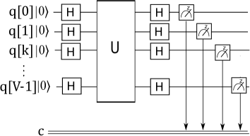
Figure 1: Quantum protocol for quantifying $|U|^{2}$ with quantum programming.

Let us consider particular case of spin system. We examine a spin chain with the following Hamiltonian

$$H_{I}=J_{01}\sigma^{z}_{0}\sigma^{z}_{1}+J_{12}\sigma^{z}_{1}\sigma^{z}_{2},$$ (21)

Weighted graph state

$$\ket{\psi(t)}=\exp\left(-\frac{itJ_{01}\sigma^{z}_{0}\sigma^{z}_{1}}{\hbar}\right)\exp\left(-\frac{itJ_{12}\sigma^{z}_{1}\sigma^{z}_{2}}{\hbar}\right)\ket{+++}$$ (22)

can be represented with a chain with three vertices $0,1,2$ and two edges $(0,1)$ $(1,2)$ characterized by weights $J_{01}$, $J_{12}$. Let us find $\langle\Delta H^{2}\rangle$ with quantum programming. For this purpose we construct quantum protocol presented in Fig. 2. In the protocol parameters $\phi_{ij}$ are related with $J_{ij}$ and time. They read $\phi_{ij}=2J_{ij}t/\hbar$. We consider $J_{01}=J$, $J_{01}=2J$. In this case we have $\phi_{01}=2Jt/\hbar=2\phi$ and $\phi_{12}=4Jt/\hbar=4\phi$, where for convenience we consider notation $\phi=Jt/\hbar$.

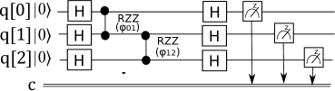
Figure 2: Quantum protocol for quantifying $|U|^{2}$ with quantum programming for spin system with Hamiltonian (21).

We run the protocol Fig. 2 on IBM’s quantum computer ibm_sherbrooke for small times. Namely we considere parameter $\phi$ in range from $-3\pi/32$ to $3\pi/32$ changing with step $\pi/64$, and number of shots equals $1024$. We fit the obtained result by $-a\phi^{2}+b$ with $a$, $b$ being constants. Taking into account relation (20), one finds $\braket{\Delta H^{2}}=aJ^{2}=4.08J^{2}$.

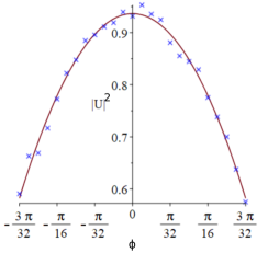
Figure 3: Results of quantum calculations of $|U|^{2}$ for spin chain (21) (marked by crosses) and fitting curve $-4.08\phi^{2}+0.94$ (represented with a line).

.

On the other hand, using (21) we can also write

$$\braket{\Delta H^{2}}=J^{2}_{01}+J^{2}_{12}+2J_{01}J_{12}\braket{\sigma^{z}_{0}\sigma^{z}_{2}}=5J^{2}+4J^{2}\braket{\sigma^{z}_{0}\sigma^{z}_{2}}.$$ (23)

One can detect the value $\braket{\sigma^{z}_{0}\sigma^{z}_{2}}=\bra{++}\sigma^{z}_{i}\sigma^{z}_{j}\ket{++}$ using quantum programming with a simple protocol. It is presented in Fig. 4. On the basis of the results of measurements in the standard basis we obtain $\bra{++}\sigma^{z}_{i}\sigma^{z}_{j}\ket{++}=|\langle{00}|++\rangle|^{2}-|\langle{01}|++\rangle|^{2}-|\langle{10}|++\rangle|^{2}+|\langle{11}|++\rangle|^{2}$.

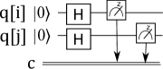
Figure 4: Quantum protocol for quantifying $\bra{++}\sigma^{z}_{i}\sigma^{z}_{j}\ket{++}$

We run the protocol Fig. 4 on ibm_sherbrooke with the number of shots $1024$. On the basis of the results of measurements, we obtain $\braket{\sigma^{z}_{0}\sigma^{z}_{2}}=0.045$. So, using (23) for $\braket{\Delta H^{2}}$ we find $\braket{\Delta H^{2}}=5.18J^{2}$. Taking into account obtained relation (7) one can also find the sum of the weighted degrees of nodes in graph $G^{(2)}(V,E)$, we have

$$\sum_{i}n_{i}^{(2)}=10.36J^{2}.$$ (24)

The theoretical result for this value reads $\sum_{i}n_{i}^{(2)}=10J^{2}$.

Similarly for $\braket{\Delta H^{3}}$ and $\braket{\Delta H^{4}}$ we can write

$$\braket{\Delta H^{3}}=(J^{3}_{01}+3J_{01}J_{12}^{2})\braket{\sigma^{z}_{0}\sigma^{z}_{1}}+(J^{3}_{12}+3J^{2}_{01}J_{12})\braket{\sigma^{z}_{1}\sigma^{z}_{2}}=1.22J^{3},$$ (25)

$$\braket{\Delta H^{4}}=J_{01}^{4}+J_{12}^{4}+6J_{01}^{2}J^{2}_{12}+4(J^{3}_{01}J_{12}+J_{01}J_{12}^{3})\braket{\sigma^{z}_{0}\sigma^{z}_{2}}=42.80J^{4}.$$ (26)

Now, taking into account the expressions for the curvature and torsion one obtains

$${\gamma^{2}\over R^{2}}=0.60,\ \ {\bar{\tau}}=0.58$$ (27)

The results are in agreement with the theoretical ones. On the basis of analytical calculations for curvature and torsion in this case we have ${\gamma^{2}/R^{2}}={\bar{\tau}}=0.64$.

4 Conclusions

Weighted graph states of the spin system described by Ising model have been studied. The velocity, curvature, and torsion of the states have been calculated with the usage of their relation with the fluctuations of energy.

We have found the relation of the fluctuations of energy and geometrical characteristics of the weighted graph states with graph properties. Namely, we have obtained that the velocity of quantum evolution is determined by the sum of the weighted degrees of nodes in the graph $G^{(2)}(V,E)$. The graph $G^{(2)}(V,E)$ is constructed by squaring the wights of graph $G(V,E)$ that represents the weighted graph state (9). The curvature (17) depends on the sum of products of weights of edges creating squares in graph $G(V,E)$ and also on the sum of the weighted degrees of nodes in the graphs $G^{(2)}(V,E)$, $G^{(4)}(V,E)$. The graph $G^{(4)}(V,E)$ can be obtained by rising to the fourth the wights of graph $G(V,E)$. The torsion in addition is determined by the sum of products of weights of edges in graph $G(V,E)$ creating triangles $S_{3}$ (19).

Geometric properties of weighted graph states have been studied with quantum programming on the basis of their relation with the fluctuations of energy. In the particular case of a spin chain (21) we have calculated the curvature and torsion (27) and also the sum of the weighted degrees of nodes in the graph $G^{(2)}$ (24) on the basis of results of programming on IBM’s quantum computer ibm_sherbrooke. The results obtained on the basis of quantum calculations are in agreement with the theoretical ones.

References

- [1] D. Brody, L. P. Hughston, Phys. Rev. Lett. 77, 2851 (1996).
- [2] H. P. Laba, V. M. Tkachuk, Condens. Matter Phys. 20, 13003 (2017).
- [3] A. Shimony, Ann. N.Y. Acad. Sci. 755, 675 (1995).
- [4] Dorje C Brody, Lane P. Hughston, J. Geom. Phys. 38, 19 (2001).
- [5] Dorje C. Brody, Anna C. T. Gustavsson, Lane P. Hughston, J. Phys.: Conf. Ser. 67, 012044 (2007).
- [6] A. M. Frydryszak, M. I. Samar, V. M. Tkachuk, The European Physical Journal D 71 (9), 1-8 (2017).
- [7] J. Anandan, Y. Aharonov, Phys. Rev. Lett. 65, 1697 (1990).
- [8] S. Abe, Phys. Rev. A 48, 4102 (1993).
- [9] A. N. Grigorenko, Phys. Rev. A 46, 7292 (1992).
- [10] Ali Mostafazadeh, Phys. Rev. Lett. 99, 130502 (2007).
- [11] C. M. Bender, D. C. Brody, Lecture Notes in Physics 789, 341 (2009).
- [12] A. R. Kuzmak, V. M. Tkachuk, J. Phys. A: Math. Theor. 49, 045301 (2016).
- [13] A. M. Frydryszak, V. M. Tkachuk, Phys. Rev. A 77, 014103 (2008).
- [14] A. R. Kuzmak, V. M. Tkachuk, Phys. Lett A 379, 1233 (2015).
- [15] D. Markham and B. C. Sanders, Phys. Rev. A 78, 042309 (2008).
- [16] D. Schlingemann and R. F. Werner, Phys. Rev. A 65, 012308 (2001).
- [17] B. A. Bell, D. A. Herrera-Martí, M. S. Tame, Nature Communications 5, 3658 (2014).
- [18] Yuanhao Wang, Ying Li, Zhang-qi Yin, Bei Zeng, npj Quant. Inf. 4, 46 (2018).
- [19] G. J. Mooney, Ch. D. Hill, L. C. L. Hollenberg, Sci. Rep. 9, 13465 (2019).
- [20] P. Mazurek, M. Farkas, A. Grudka et al Phys. Rev. A 101, 042305 (2020).
- [21] N. Shettell, D. Markham Phys. Rev. Lett. 124, 110502 (2020).
- [22] M. Hein, J. Eisert, H. J. Briegel, Phys. Rev. A 69, 062311 (2004).
- [23] O. Gühne, G. Tóth, Ph. Hyllus, H. J. Briegel, Phys. Rev. Lett. 95, 120405, (2005).
- [24] Y. Qian, Z. Shen, G. He, and G. Zeng, Phys. Rev. A 86, 052333 (2012).
- [25] A. Vesperini, R. Franzosi. Adv. Quantum Technol. 7, 2300264 (2024).
- [26] A. Vesperini Ann. Phys. 457, 169406 (2023).
- [27] Kh. P. Gnatenko, H. P. Laba, V. M. Tkachuk Phys. Lett. A 452, 128434 (2022)
- [28] Kh. P. Gnatenko V. M. Tkachuk, Phys. Lett. A 396, 127248 (2021).
- [29] C. Zoufal, A. Lucchi, S. Woerner. npj Quant. Inf. 5, 103 (2019).
- [30] X. Gao, Z.-Y. Zhang, L.-M. Duan. Sci. Adv. 4, 12 (2018)
- [31] Alba Cervera-Lierta J. I. Latorre, D. Goyeneche, Phys. Rev. A 100, 022342, (2019).
- [32] R. Mezher, J. Ghalbouni, J. Dgheim, D. Markham, Phys. Rev. A 97, 022333 (2018).
- [33] A. Akhound, S. Haddadi, Mohammad Ali Chaman Motlagh Mod. Phys. Lett. B 33, 1950118 (2019).
- [34] S. Haddadi, A. Akhound, Mohammad Ali Chaman Motlagh Int. J. Theor. Phys. 58, 3406 (2019).
- [35] A. Cabello, A. J. Lopez-Tarrida, P. Moreno, J. R. Portillo Phys. Lett. A 373, 2219 (2009).
- [36] Kh. P. Gnatenko, N. A. Susulovska EPL (Europhys. Lett.) 136, 40003 (2021).
- [37] N. A. Susulovska Geometric measure of entanglement of quantum graph states prepared with controlled phase shift operators arXiv:2401.14997 (2024).
- [38] Kh. P. Gnatenko Entanglement of multi-qubit states representing directed networks and its detection with quantum computing arXiv:2407.09990 (2024)
- [39] IBM Q experience. https://quantum-computing.ibm.com/