Accreting companion occurrence rates using a new method to compute emission-line survey sensitivity: application to the H$\alpha$ Giant Accreting Protoplanet Survey (GAPlanetS)

Abstract

A key scientific goal of exoplanet surveys is to characterize the underlying population of planets in the local galaxy. In particular, the properties of accreting protoplanets can inform the rates and physical processes of planet formation. We develop a novel method to compute sensitivity to protoplanets in emission-line direct-imaging surveys, enabling estimates of protoplanet population properties under various planetary accretion and formation theories. In this work, we specialize to the case of H$\alpha$ and investigate three formation models governing the planetary-mass-to-mass-accretion-rate power law, and two accretion models that describe the scaling between total accretion luminosity and observable H$\alpha$ line luminosity. We apply our method to the results of the Magellan Giant Accreting Protoplanet Survey (GAPlanetS) to place the first constraints on accreting companion occurrence rates in systems with transitional circumstellar disks. We compute the posterior probability for transitional disk systems to host an accreting companion ($-8\leq\log M\dot{M}[M_{J}^{2}\,\rm{yr}^{-1}]\leq-2$) within 2 arcseconds ($\sim 200$ au). Across accretion models, we find consistent accreting companion rates, with median and one-sigma credible intervals of $0.15^{+0.18}_{-0.10}$ and $0.19^{+0.23}_{-0.12}$. Our technique enables studying protoplanet populations under flexible assumptions about planet formation. This formalism provides the statistical underpinning necessary for protoplanet surveys to discriminate among formation and accretion theories for planets and brown dwarfs.

1 Introduction

While theoretical and observational studies over the past half century have constrained many aspects of planet formation, various mechanisms remain plausible for the formation of the wide-separation ($\sim 10-1000$ au) giant planets and brown dwarfs detected via exoplanet direct imaging (e.g., Toomre, 1964; Safronov, 1972; Reipurth & Clarke, 2001; Stamatellos & Whitworth, 2009; Lambrechts & Johansen, 2012; Forgan & Rice, 2013; Stamatellos & Herczeg, 2015; Vigan et al., 2017; Bowler et al., 2020; Do Ó et al., 2023). Robust limits on occurrence rates and parameter distributions of fully-formed, widely-separated giant planets have been made by recent large-scale direct imaging campaigns such as the Gemini Planet Imager Exoplanet Survey (Nielsen et al., 2019) and the SPHERE Infrared Exoplanet survey (Vigan et al., 2021).

Protoplanets that are actively accreting matter provide direct windows into the early stages of planet formation, making them ideal targets for discriminating among formation theories. Young stars with “transitional” disks, which host large central cavities thought to be cleared by forming planets (Lin & Papaloizou, 1993; Dodson-Robinson & Salyk, 2011; Price et al., 2018; Close, 2020), have proven fruitful targets for protoplanet imaging. Recent surveys of these have revealed a number of protoplanets and candidates (e.g. Zurlo et al., 2020; Haffert et al., 2021; Huélamo et al., 2022; Follette et al., 2023). Dedicated second-generation protoplanet imaging surveys (Close et al., 2020; Zhou et al., 2021a; Chilcote et al., 2022) will continue to increase their numbers.

However, circumstellar environments present challenges for detection and validation of protoplanet candidates. Complex disk morphologies impede ready separation of disk and planet signals (Follette et al., 2017; Currie et al., 2019). As such, of all candidates reported within circumstellar disk gaps, only PDS70 b and PDS70 c (Keppler et al., 2018; Haffert et al., 2019; Wang et al., 2021; Zhou et al., 2021b) are considered unambiguous protoplanets, while the natures of numerous others remain debated (e.g., but not limited to, Kraus & Ireland, 2012; Reggiani et al., 2014; Sallum et al., 2015; Follette et al., 2017; Rameau et al., 2017; Currie et al., 2019; Gratton et al., 2019; Currie et al., 2022; Zhou et al., 2022; Hammond et al., 2023; Biddle et al., 2024; Currie, 2024).

The challenges of protoplanet imaging mean survey results are biased toward the brightest, most easily detectable objects: those most massive and strongly accreting. To understand planet formation in full, we must conduct population inference based on survey results. This necessitates rigorous accounting for selection effects. Specifically, population studies must quantify the completeness to planets, or selection function: the proportion of planets that could have been detected around survey stars as a function of the planets’ physical properties. A method to estimate completeness for fully-formed ($\gtrsim 10$ Myr) directly-imaged planets, based on contrast limits and models for planet orbits and luminosities, has been developed over the past $\sim 15$ years (e.g. Biller et al. 2007; Nielsen et al. 2008; Wahhaj et al. 2013; Bowler 2016; Nielsen et al. 2019; Vigan et al. 2021). In advance of next-generation protoplanet imaging surveys, it is critical to formulate statistical methods to estimate the selection function for protoplanets, thereby facilitating constraints on the rates and processes of planet formation.

The critical difference between fully-formed planets and protoplanets for computing selection effects is in estimating intrinsic luminosity from mass. This is because protoplanet luminosity includes contributions from the protoplanetary photosphere, infalling accreting material, and planetary surface shock. These must be disentangled to infer the underlying properties of the object. Moreover, most protoplanet candidates have been sought and detected only in narrowband accretion-tracing spectral emission lines where protoplanets’ brightnesses are enhanced relative to those of their host stars (and the photospheric contribution is assumed to be negligible). H$\alpha$, which is both bright and accessible from the ground, is a common choice. To compute detection probabilities (and therefore population properties) for protoplanets in narrowband imaging data requires modeling how protoplanets’ masses and accretion rates manifest in the observed luminosities of accretion-tracing spectral lines. Section 2 details how this is a function of (1) the formation condition of the object and its disk and (2) the mechanism of accretion onto the object.

In this article, we present a method to compute survey sensitivity to accreting protoplanets under flexible assumptions about formation and accretion, enabling the first statistical study of protoplanet population properties. Section 2 outlines the models for planet formation and accretion we apply to our dataset. In Section 3, we describe the Magellan Giant Accreting Protoplanet Survey (GAPlanetS, Follette et al., 2023), the survey used for our analysis. Section 4 describes our Monte Carlo simulation technique for computing completeness. We present a general framework, then implement the astrophysical models of Section 2, and apply the technique to GAPlanetS data. We report and discuss our constraints on protoplanet occurrence rates in Section 5 before concluding in Section 6.

2 Planet formation and accretion

Computing the probability of detecting a planet of given physical properties requires converting its physical parameters to those observed, then comparing its observable characteristics to a threshold for detection. In protoplanet high-contrast imaging, the measurable parameters are (1) projected angular separation (in milliarcseconds (mas)) and (2) planet-to-star line luminosity ratio (contrast; here, we consider imaging at H$\alpha$). The physical properties of interest, on the other hand, are (1) semimajor axis $a$, (2) mass $M$, and (3) mass accretion rate $\dot{M}$. It is worth noting that estimating selection effects from models and interpreting observational data require opposite chains of models. Computing completeness requires forward-modeling from physical parameters to observable ones, while interpreting observations requires statistically linking the data to the physical properties. For protoplanets, the mass maps to the observable ($L_{\mathrm{H}\alpha}$, assuming $L_{\mathrm{H}\alpha}$ of the star is known) according to the following schema:

$$M\to M\dot{M}\to L_{\mathrm{acc}}\to L_{\mathrm{H}\alpha}.$$ (1)

The relevant equation for each step of this mapping depends on the processes that formed the object and on its accretion mechanism. The formation condition determines the mass of the circumsecondary disk surrounding an accreting object—i.e., the amount of matter available for accretion—which subsequently controls the expected accretion rate of a companion of a given mass. The accretion mechanism governs the fraction of total accretion emission that escapes in the observed spectral line.

The astrophysical models we employ at each step are detailed in the remainder of this section. For each, we compare one “stellar” model, derived from empirical data, and one theoretically-derived “planetary” model. We then compute completeness following a Monte Carlo procedure that implements these steps, shown schematically in Figure 1. The simulation details are in Section 4.

More specifically, Section 2.1 summarizes current observational evidence for a power-law relation between object mass and mass accretion rate, the first step in Schema 1. In Section 2.2, we describe how the slope and spread of this relation reflects the formation pathway of the planets and their disks. We then introduce two formation models we chose for this work. The relation between $M\dot{M}$ and accretion luminosity $L_{\mathrm{acc}}$ (the second step of Schema 1) follows classic assumptions for gravitational infall (Section 2.3). Section 2.4 describes the models we adopt in this work for the proportion of total accretion luminosity $L_{\mathrm{acc}}$ that escapes in H$\alpha$ (the third step of Schema 1). This fraction depends on the physical properties of the accretion flow. Finally, in Section 2.5 we describe how a companion’s projected separation is a function of the system’s orbital parameters, a computation that closely follows established methods.

With this framework, we can compute observable characteristics of protoplanets as a function of semimajor axis $a$ and mass $M$ under any combination of model assumptions for formation and accretion. We combine these observable characteristics with survey detection thresholds to compute completeness to protoplanets, and estimate population properties, under an assumed model. Moreover, with hierarchical inference, this framework can be used to infer the model parameters themselves.

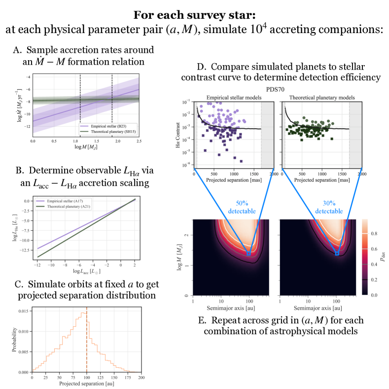
Figure 1: Steps to estimate direct-imaging survey completeness to accreting companions. At each physical parameter set $(a,M)$, we simulate $10^{4}$ accreting companions. First, we sample mass accretion rates $\dot{M}$ using an assumed model for the $\dot{M}\textrm{--}M$ scaling. Step A shows the models in Section 2.2; the stellar model is in purple and the planetary in green. Next, we convert each $M\dot{M}$ to $L_{\mathrm{acc}}$ (Section 2.3). We then compute the observable $L_{\mathrm{H}\alpha}$ based on a model for the accretion scaling; Step B shows the two models in Section 2.4. We obtain the projected separation distribution by sampling companion orbital parameters as in Section 2.5; Step C shows one such distribution for an object at $a=100$ au. Finally, we compare the simulated companions to the survey star’s contrast curve to estimate the detectable fraction. Step D shows two examples of 100 brown dwarfs $(a,M)=(100\,\mathrm{au},\,26\,M_{J})$ around PDS70; the left panel shows companions simulated using both “stellar” models, while the right uses both “planetary” models. We repeat across a grid in $(a.M)$ for each combination of models to obtain the entire completeness maps (Step E).

2.1 Observational evidence for the relation between $M$ and $\dot{M}$

The relation between young stars’ masses and mass accretion rates follows an empirically-established power law, $\dot{M}\propto M^{\gamma}$, $\gamma\approx 2$ (Alcalá et al., 2017; Betti et al., 2023; Almendros-Abad et al., 2024). The steep observed $\dot{M}\textrm{--}M$ scaling is consistent with simple models of molecular cloud core collapse followed by viscous disk evolution (e.g. Dullemond et al., 2006).

In the substellar regime, however, this relation is not as secure, and has significant scatter of 1–2 dex (Alcalá et al., 2017; Betti et al., 2023; Almendros-Abad et al., 2024). The high scatter of the single power-law model motivated alternate ways of describing the relation at substellar masses. For example, Muzerolle et al. (2005), Manara et al. (2017), and Alcalá et al. (2017) find observations are best fit by a broken power law, with a steeper index $\gamma$ for isolated brown dwarfs than stars.

Observations of accreting planetary-mass companions (PMCs)—brown dwarfs and protoplanet candidates bound to higher-mass stars—indicate higher accretion rates with weaker dependence on object mass than predicted by either single or broken power laws (e.g. Sallum et al., 2015; Haffert et al., 2019; Betti et al., 2022). This is suggestive of formation by disk fragmentation (see Section 2.2.2 and Stamatellos & Herczeg 2015). To assess the effects of systematic errors on $\dot{M}\textrm{--}M$ scatter and the best-fit power law(s), Betti et al. (2023) re-derived mass accretion rates for 798 low-mass and substellar objects from the literature under a uniform set of stellar distance and age estimates, empirical scaling relations, and pre-main sequence evolutionary models. Despite reduction of systematics, the data remain best fit with a break in the slope of the $\dot{M}\textrm{--}M$ relation at the substellar boundary, and by fitting jointly for mass and age.

2.2 $\dot{M}\textrm{--}M$ as a probe of formation pathways

A likely explanation for the fact that current data are best described by an overlapping set of $\dot{M}\textrm{--}M$ power laws is that the data comprises multiple subpopulations defined by distinct formation conditions. An accreting object’s initial environment influences the mass of its surrounding disk, which governs the relation between its mass and mass accretion rate. However, resolving separate formation channels is complicated by intrinsic accretion variability and observational uncertainty, hence substellar mass-to-mass-accretion rate power laws remain an active area of observational and theoretical research. Moreover, the observational evidence for multiple formation pathways remains entangled with systematics of accretion calculations, some of which rely on assumptions that are untested at substellar masses.

The $\dot{M}\textrm{--}M$ power law is key for estimates of completeness because contrast is proportional to $M\dot{M}$. As the nature of this relation is a subject of ongoing research, we provide a generalized framework for calculations of survey sensitivity. Sections 2.2.1–2.2.3 outline three possible approaches that cover a range of substellar formation scenarios in current literature. In this work, we compute survey sensitivity assuming each model in turn; inferring the relative importance of each model, or inferring the power law parameters, will be the subject of future work.

2.2.1 Empirical stellar relation

A protoplanet on a stable orbit that cleared a large gap in the circumstellar disk, or one that formed as a quasi-binary companion, may have access to a limited reservoir of material for accretion set by its initial mass. A reasonable proxy for the resultant $\dot{M}\textrm{--}M$ relation is the single power law fit from CASPAR:

$$\log\dot{M}/(M_{\odot}\text{yr}^{-1})=2.05\log M/M_{\odot}-7.98$$ (2)

which has an associated spread of $\sigma=0.97$ dex.

This relation predicts a steep drop-off of accretion rate with mass ($\gamma\approx 2$), though with high scatter of $\approx 1$ dex. Because the data underlying this fit are empirical, we emphasize that Equation 2 is not derived from stellar formation physics, but instead reflects the scenario of a system with a fixed mass reservoir set early in its formation. We subsequently cite Betti et al. (2023) as B23 and refer to Equation 2 as the “isolated” or “empirical stellar” formation model.

2.2.2 Theoretical planetary relation

An alternate model for formation of substellar companions is via fragmentation of a massive, gravitationally unstable circumstellar disk. Simulations of disk fragmentation suggest the resulting circumsecondary disks are more massive than independent evolution would dictate because the disks draw matter from the natal system for longer (Stamatellos & Herczeg, 2015). Since accretion rate scales with disk mass, both for companions and isolated accretors (Manara et al., 2016; Somigliana et al., 2022; Fiorellino et al., 2022), disk fragmentation simulations predict protoplanets with higher accretion rates that are more weakly dependent on object mass than the empirical stellar relation.

Disk evolution modeling requires the disk viscosity $\alpha$, which governs the rate of angular momentum transport. As lower viscosity disks evolve more slowly, the fragments that form circumplanetary disks pull more mass from the natal system, and their planets consequently have higher accretion rates. Indeed, Rafikov (2017) finds observational evidence for a correlation between $\alpha$ and $\dot{M}$. Following Stamatellos & Herczeg (2015), Rafikov (2017), and Somigliana et al. (2022), we assume $\alpha$ does not depend on object mass and use the presumed value for T-Tauri stars, $\alpha=0.01$. We adopt the $\dot{M}\textrm{--}M$ scaling with these assumptions from the simulations of Stamatellos & Herczeg (2015), henceforth SH15:

$$\log\dot{M}/(M_{\odot}\text{yr}^{-1})=0.12\log M/M_{\odot}-10.5,$$ (3)

which has a spread of $\sigma=0.3$ dex.

Compared to Equation 2, Equation 3 has a shallower slope ($\gamma=0.12$) and less variation in accretion rate ($\sigma=0.3$ dex). We subsequently refer to Equation 3 as the “fragmentation” or “planetary” formation model. Such a flat relation between $M$ and $\dot{M}$ is useful from a detection standpoint, as it implies better contrasts for low-mass objects. However, it impedes source classification and demographics: an observed $M\dot{M}$ (computed from contrast) has more pronounced degeneracy between $M$ and $\dot{M}$ than if there were a stronger correlation.

2.2.3 Formation-agnostic

Observationally, single measurements of H$\alpha$ contrast constrain only the ratio $M\dot{M}/R$ (see Equation 4). Separately constraining $M$ and $\dot{M}$ requires multiwavelength observations. As several GAPlanetS protoplanet candidates have only $M\dot{M}$ constraints, we also outline a conservative approach that avoids assuming an $\dot{M}\textrm{--}M$ scaling. For this scenario, we consider the product $M\dot{M}$ to be the physical parameter, which makes our completeness maps “agnostic” about the relation between $M$ and $\dot{M}$. The product $M\dot{M}$ has been used when observing other quantities dependent on both mass and accretion, such as the flux density of dust continuum emission (Shibaike & Mordasini, 2024).

While this approach reduces one assumption, it does not enable inference about the relative frequencies of formation processes, which requires separate estimates of $M$ and $\dot{M}$. In anticipation of more robust protoplanet mass estimates in the future, we demonstrate computation of protoplanet survey completeness under the two $\dot{M}\textrm{--}M$ relations outlined above, though we do not compare the GAPlanetS candidates to these results.

2.3 Total accretion luminosity

In the standard model for stellar accretion, the circumstellar disk is truncated by the star’s magnetic field at a radius $R_{\textrm{m}}$ (e.g., Koenigl, 1991). Accreting matter flows in columns along magnetic field lines from $R_{\textrm{m}}$ to the stellar surface at near free-fall velocity, causing an accretion shock. The resulting accretion luminosity $L_{\mathrm{acc}}$ is given by:

$$L_{\mathrm{acc}}=\frac{GM\dot{M}}{R}\left(1-\frac{R}{R_{\textrm{m}}}\right).$$ (4)

Computing $L_{\mathrm{acc}}$ thus requires estimates for the truncation radius $R_{\textrm{m}}$ and object radius $R$. We use the classic estimate $R_{\textrm{m}}=5R$, a value consistent with observations (Calvet & Gullbring, 1998; Hartmann et al., 2016). While a different dependence of $L_{\mathrm{acc}}$ on $M\dot{M}$ may apply for non-magnetospheric accretion processes (e.g. Aoyama et al., 2021), we note that a modification of Equation 4 should add only an overall scale factor to our completeness estimates. We expect uncertainty in this relation to be subdominant compared to uncertainties in Equations 2 and 3.

We also assume a uniform value for planet radius, namely $2R_{J}$. Alternately, planet radii can be modeled as a function of mass and mass accretion, as done in Aoyama et al. (2020) using data from Mordasini et al. (2012). Their results agree with the population synthesis results of Emsenhuber et al. (2021). However, Aoyama et al. (2020) find protoplanet radii vary only by a factor of two in our parameter space ($\log M[M_{J}]\in[0,2],\;\log\dot{M}[M_{J}\mathrm{yr}^{-1}]<-5$), so the impact of radius uncertainty on the inferred completeness estimates is likely small. In this work, we focus on comparing models for the $\dot{M}\textrm{--}M$ and $L_{\mathrm{H}\alpha}\textrm{--}L_{\mathrm{acc}}$ relations. However, incorporating the Aoyama et al. (2020) fit for $R(M,\dot{M})$ or comparing models for the radius relation is an extension that may better reflect planet characteristics.

2.4 Accretion mechanisms and H$\alpha$ emission

Measuring $L_{\mathrm{acc}}$ provides the most direct way to estimate $\dot{M}$ in principle, but it often cannot be measured in practice. Accretion emission is primarily in the near-UV continuum, with substantial line luminosity contributions in the mid-to-far UV, optical, and near-infrared. Since multiwavelength observations for low-mass and substellar objects have not yet been obtained in most cases, spectral lines such as H$\alpha$ are often used as secondary tracers of accretion (e.g. Alcalá et al., 2014, 2017; Natta et al., 2006; Manara et al., 2015).

The nature of the accretion flows impacts how the total accretion luminosity is partitioned across the electromagnetic spectrum. For a given rate of accretion, how much is radiated in H$\alpha$ thus depends on the mechanism of accretion. Since planetary accretion physics are not well constrained, we compare two models for how $L_{\mathrm{H}\alpha}$ scales with $L_{\mathrm{acc}}$: one empirically derived from observations of low-mass stars, and one theoretically derived from simulations of accretion flows onto planets.

Interpreting H$\alpha$ observations requires knowledge, or assumption, of the applicable accretion scaling relation. As identifying the scaling for any given system remains an observational challenge, we compute completeness to GAPlanets under both relations, enabling comparing the population inference using each assumption.

2.4.1 Empirical stellar relation

In low-mass stars where both accretion line emission and UV excess (as a proxy for $L_{\mathrm{acc}}$) can be measured simultaneously, empirical correlations have been derived for the relation between line and accretion luminosity. Here we consider the $L_{\mathrm{H}\alpha}\textrm{--}L_{\mathrm{acc}}$ relation determined in Alcalá et al. (2017) (hereafter A17), namely:

$$\log L_{\mathrm{acc}}/L_{\odot}=1.13\times\log L_{\mathrm{H}\alpha}/L_{\odot}+1.74.$$ (5)

We note that A17 recommend the use of other accretion tracers over H$\alpha$, in part because of the high observed dispersion, thought to be due to other processes (e.g. outflows, magnetic fields) that contribute to $L_{\mathrm{H}\alpha}$. However, since H$\alpha$ is one of the only ground-accessible accretion tracers observable at planetary fluxes, it is a necessary, though imperfect, choice. The low-mass stars described by Equation 5 accrete magnetospherically. During magnetospheric accretion, this line emission is believed to originate from the accretion columns, with the infalling gas producing broad emission lines. The accretion shock onto a stellar surface is almost entirely ionized, creating primarily hot continuum emission and little line emission (Hartmann et al., 2016).

2.4.2 Theoretical planetary relation

In the planetary accretion case, infalling material may be too cool to emit substantially at H$\alpha$, and the post-shock region may be cool enough to maintain bound elections. Thus line emission may originate primarily from the photospheric post-shock region, which contributes to a lower H$\alpha$ production efficiency. Additionally, planets may not have sufficiently strong magnetic fields to accrete magnetospherically, instead exhibiting “boundary layer accretion” (e.g. Fu et al. 2023).

Aoyama et al. (2021) (hereafter A21) quantified the expected H$\alpha$ emission of a planetary accretion shock via non-equilibrium radiation-hydrodynamic simulations combined with a simple estimate for the accretion geometry and found:

$$\log L_{\mathrm{acc}}/L_{\odot}=0.95\times\log L_{\mathrm{H}\alpha}/L_{\odot}+1.61,$$ (6)

which, compared to Equation 5, predicts less H$\alpha$ emission for a given $L_{\mathrm{acc}}$.

The fit of Equation 6 was obtained in the limit of azimuthally-symmetric accretion onto a planet, assuming a shock only at the planetary surface. In a more realistic accretion geometry (e.g., Tanigawa et al., 2012), the circumplanetary disk surface shock will also add to the line flux (Aoyama et al., 2018), but its contribution is likely subdominant compared to the photospheric shock (Marleau et al., 2023).

While the scaling relations Equations  5 and 6 nominally delineate “stellar” and “planetary” accretion processes, either mechanism may apply for a given substellar object. Indeed, observations of PDS70 b imply a high fraction of accretion emission at H$\alpha$, with such efficient production suggesting a more “stellar” accretion process (Zhou et al., 2021b). Upcoming studies of the PDS70 system hope to further unveil the process at play (Aoyama et al., 2022). Similarly, measurements of the number density of the accretion flow onto Delorme 1 (AB)b imply a small line-emitting area, suggesting the accretion flow is a column (Betti et al., 2022; Ringqvist et al., 2023).

2.5 Modeling planetary orbits

For consistency with previous work (e.g. Nielsen et al. 2019), we compute detectability as a function of semimajor axis marginalized over other orbital parameters. To model companions’ orbits, we use the typical assumption of isotropy in viewing angle and most orbital characteristics: we model inclination angle $i$ as uniform over $\cos(i)\in[-1,1]$; argument of periastron $\omega$ as uniform in $\omega\in[0,2\pi]$; and epoch of periastron passage $\tau$, expressed as fraction of orbital period past a reference time, as uniform over $\tau\in[0,1]$. The position angle of nodes, which sets an orbit’s azimuthal orientation, is not simulated as GAPlanetS contrast curves are azimuthally averaged.

The eccentricity distribution of exoplanets is less well constrained. Planet population studies have employed a range of possibilities, and recent studies have put new constraints on the distribution. Nielsen et al. (2019) uses $P(e)\propto 2.1-2.2e,\,0\leq e\leq 0.95$, derived from the radial velocity survey of Butler et al. (2006). Bowler et al. (2015) compares results using circular orbits ($e=0$) to those using a nearly-identical distribution to Nielsen et al. (2019), $P(e)\propto 1-e$, which is based on a combination of radial velocity and M-dwarf binary observations (Duchêne & Kraus, 2013; Kipping, 2013). More recent work by Bowler et al. (2020) fit the eccentricities of imaged giant planets and brown dwarfs to Beta distributions and found a dependence on companion mass and orbital period. They interpret these trends as evidence for different formation channels, which suggests the proper eccentricity model may depend on the formation condition. The population study of Vigan et al. (2021) uses the best-fit parameters for the entire sample of Bowler et al. (2020) ($\alpha=0.95$, $\beta=1.30$). Do Ó et al. (2023) fits a sub-sample of objects from Bowler et al. (2020), finding Beta parameters $\alpha=1.09$, $\beta=1.42$, a nearly uniform distribution. Wahhaj et al. (2024) finds $e\approx 0.5$ for PDS70 b and c, suggesting high eccentricities are possible for protoplanets.

To assess the importance of the assumed eccentricity distribution, we compare two possible distributions. As a conservative possibility, we assume all orbits have circularized; i.e., $P(e)=\delta_{0,e}$. As a second possibility, we follow Nielsen et al. (2019) and use $P(e)\propto 2.1-2.2e,\,0\leq e\leq 0.95$.

With models for $\dot{M}\textrm{--}M$ and $L_{\mathrm{H}\alpha}\textrm{--}L_{\mathrm{acc}}$, such as those in Sections 2.2–2.4, we perform the schematic mapping 1 and compute the luminosity of a protoplanet. Using the orbital models here, we compute the projected separation. This completes the requirements for translating physical to observable parameters. In the remainder of this article, we apply this framework to real observations from GAPlanetS (Follette et al., 2023) to compute survey completeness.

3 Data

The Giant Accreting Protoplanet Survey collected H$\alpha$ images of 14 transitional disk systems with the Magellan Adaptive Optics (Close et al., 2013; Morzinski et al., 2014, 2016) system. GAPlanetS sample selection, data collection, reduction, and analysis pipelines are detailed in Follette et al. (2023) and Adams Redai et al. (2023).

Since our aim is planet demographics, we must define the stellar population on which we are performing inference. GAPlanetS is a highly targeted survey: it selected stars with transitional disks hosting large ($>0\farcs 1$), cleared central cavities visible from the Magellan telescope ($\delta<25\,\deg$) and of sufficiently brightness for observation with natural guide star adaptive optics (rmag$<$12). Our inference about protoplanet populations is thus limited to gapped transitional disk host stars. While this is a sampling bias, it is also a consequence of the fact that we expect forming planets to be most prevalent inside disk gaps and cavities.

GAPlanetS reported six detections of accreting companions and candidates in five systems. Two (HD142527 B, HD100453 B) are low-mass stars. Although not protoplanets, their formation environments may be analogous to substellar companions, which motivates studying their formation and accretion properties (Balmer et al., 2022). GAPlanets recovered the confirmed protoplanet PDS70 c and candidates LkCa 15 b and CS Cha c. They did not robustly recover PDS70 b, so we exclude it from this analysis.

They computed the detection threshold as a function of separation, or contrast curve, for each epoch of observation for each star. Contrast curves are determined via injection and recovery of false planets at fixed contrasts. After injection, the stellar PSF is modeled and subtracted via pyKLIP (Wang et al., 2015) using the optimization process described in Adams Redai et al. (2023) and Follette et al. (2023). In these post-processed images, the detection threshold is set using the remaining 5$\sigma$ image noise corrected for small sample statistics at low separations (Mawet et al., 2014) and multiplied by the algorithm throughput (the ratio between injected and post-pyKLIP planet flux). As a caveat, we note that the method of Mawet et al. (2014) was generalized to non-Gaussian noise in Bonse et al. (2023), whose results suggest the Gaussian assumption is too optimistic.

The relevant stellar parameters to compute completeness for each survey star are given in Table 1. We compare the simulated companions to the optimized contrast curves for each survey star. This gives the detection probability for each star as a function of companion parameters, conditioned on the astrophysical models.

Star	$M$ [$M_{\odot}$]	$d$ [pc]	$m_{r^{\prime},\star}$ [mag]	$A_{r^{\prime},\star}$ [mag]	$S$
HD100546	2.4	108.1	6.8	0.2	1.59, 1.43
HD141569	2.39	111.6	7.2	0.2	0.94, 0.96, 0.95, 0.92, 0.92
HD100453	1.7	103.8	7.8	0.2	1.05, 1.26, 1.04, 1.10
HD142527	2.0	159.3	8.2	0.8	1.13, 0.88, 1.12, 1.14, 1.22, 1.28, 1.13, 1.14
HD169142	1.85	114.9	8.2	0.0	1.06, 0.98, 0.99, 1.13
SAO206462	1.7	135.0	8.6	0.1	1.22, 1.22
V1247Ori	1.86	401.3	9.9	0.3	1.13, 1.12
PDS66	1.4	97.9	10.0	0.7	1.91
V4046Sgr	1.75	71.5	10.0	0.0	1.80, 1.79
TWHya	0.6	60.1	10.5	0.5	8.79, 7.17
CSCha	1.32	168.8	11.1	1.0	2.26
UXTauA	1.25	142.2	11.3	0.5	1.42
LkCa15	1.25	157.2	11.6	0.5	1.81, 1.58
PDS70	0.82	112.4	11.7	0.0	1.29, 1.36, 1.32

Table 1: Selected parameters of GAPlanetS survey stars. From left to right, stellar mass in solar masses, distance in parsecs, apparent $r^{\prime}$ band magnitude, $r^{\prime}$ band extinction, and H$\alpha$-to-continuum scale factor for each observational epoch, ordered by epoch. Additional parameters, and how each was determined, are given in Tables 2 and 5 and Section 6 of Follette et al. (2023).

4 Method to compute completeness

We determine GAPlanetS’ completeness to accreting companions following a Monte Carlo procedure. For each target star, we compute completeness on a 60x60 grid. We use a log-uniform grid in semimajor axis ranging from 1 to 500 au. For the y-axis, we use either the log of mass in the range $\log M\in[0,2.5]\log M_{J}$, or the log of the product $M\dot{M}$, $\log M\dot{M}\in[-10,-2]\log M_{J}^{2}\,\rm{yr}^{-1}$. These ranges span planets, brown dwarfs, and the lowest-mass stars. We assume log-uniform priors on $a$ and $M$ (or $M\dot{M}$). At each set of parameters $(a,M)$ or $(a,M\dot{M})$, we simulate $10^{4}$ companions. We determine the fraction detectable by estimating the observable parameter distribution $p(\mathrm{separation},L_{\mathrm{H}\alpha})$ for the given physical parameters. We do so by simulating companion orbits and $L_{\mathrm{H}\alpha}$, the latter of which depends on the scaling law for each step in Schema 1.

Here, we consider the three models for $\dot{M}\textrm{--}M$ in Section 2.2 and the two $L_{\mathrm{H}\alpha}\textrm{--}L_{\mathrm{acc}}$ scaling laws outlined in Section 2.4. The stellar H$\alpha$ luminosities are taken from the GAPlanetS survey, which we use to compute the contrast of each simulated companion. To determine the distribution of projected separation, we randomly assign orbital parameters to each companion. Finally, we label each simulated companion as “detectable” or “undetectable” in GAPlanetS data by comparing its separation and contrast to the target star’s contrast curve. The steps in our simulations are diagrammed as a flowchart in Figure 1 and further described in Sections 4.3–4.4.

4.1 Simulating accretion rates

Although protoplanet detections in accretion tracing lines place minimal direct constraints on planet mass, we can estimate mass limits from accretion rate limits by assuming a relation between $M$ and $\dot{M}$. In this work, we employ the two $\dot{M}\textrm{--}M$ relations described in Section 2.2: the empirical stellar power law of B23, Equation 2, and the theoretical fragmentation model of SH15, Equation 3. These “star-like” and “planet-like” power laws are shown in Step A of Figure 1 in purple and green, respectively. At planetary masses, objects that form from a fragmented disk are easier to detect, as the model predicts higher accretion rates, thus higher luminosities, than for objects of the same mass formed by the stellar model. At brown dwarf masses, the relations overlap.

When simulating $M\dot{M}$ in the formation-agnostic case, we directly compute $L_{\mathrm{acc}}$ from Equation 4, and then compute $L_{\mathrm{H}\alpha}$ using either Equation 5 or 6.

In all cases, we assume freefall from a truncated circumplanetary disk and thus use Equation 4 to convert from $M\dot{M}$ to $L_{\mathrm{acc}}$. As discussed in Section 2.4, we assume a uniform planet radius of $2R_{J}$. Since $M/R$ varies far less than $\dot{M}$ between objects, we expect error introduced by assuming a constant radius to be subdominant.

4.2 Computing H$\alpha$ luminosity

We compute completeness under the two models for $L_{\mathrm{H}\alpha}\textrm{--}L_{\mathrm{acc}}$ described in Section 2.4: the empirical stellar fit of A17 (our Equation 5), and the planetary hydrodynamic simulation results from A21 (our Equation 6), shown in Step B of Figure 1. As before, the stellar model is in purple and the planetary in green. The planetary model predicts less efficient H$\alpha$ production than the stellar model in our range of interest, so objects that “accrete like a planet” are harder to detect than objects with the same $M\dot{M}$ that accrete magnetospherically.

4.3 Orbital distributions

As discussed in Section 2.5, we sample most orbital parameters from independent isotropic distributions. With a set of parameters $[a,i,\omega,\tau,e]$, we compute projected separation from the Keplerian orbit parameters (Blunt et al., 2020). An example projected separation distribution for a companion at 100 au (using $P(e)\propto 2.1-2.2e$) is shown in Step C of Figure 1.

4.4 Detectability

Following Follette et al. (2023), we compute each simulated companion’s contrast via

$$\log C=\log\frac{L_{\mathrm{H}\alpha}}{4\pi d^{2}z\Delta\lambda}+\frac{m_{r^{\prime},\star}-A_{r^{\prime},*}}{2.5}-\log S,$$ (7)

where $z$ is the instrumental zero point; $\Delta\lambda$ the effective filter width; $d$ the distance to the star; $m_{r^{\prime},\star}$ and $A_{r^{\prime},\star}$ the star’s apparent magnitude and extinction, respectively, in $r^{\prime}$ band, which is a good proxy for the H$\alpha$ continuum values; and $S$ the star’s H$\alpha$-to-continuum scale factor. For the Magellan Clay telescope, used by GAPlanetS, $z=1.733\times 10^{-5}\;\text{erg cm}^{-2}\text{ s}^{-1}\;\upmu\text{m}^{-1}$ and $\Delta\lambda=6.3$ nm (Males, 2013). The values of each parameter for each star is provided in Table 1. Details of the derivation of each, and additional parameters, are in Tables 2 and 5 and Section 6 of Follette et al. (2023).

We compare each set of simulated companions to each survey star’s contrast curve(s). Many of the survey stars were observed in multiple epochs. Since contrast curves vary between observation nights, a companion may be revealed or drop sub-threshold. If a simulated companion is above at least one contrast curve, it is labeled “detectable”. We do not evolve the companions’ orbits between epochs. Since the distribution of projected separation will not change with orbital evolution, it will not affect the aggregate detectable fraction. Further, accretion rates are known to vary on short and long timescales. Since the stochastic accretion rate variability is unknown, we cannot deterministically predict how an object’s assigned $M\dot{M}$ may change between epochs; however, the overall distribution of $M\dot{M}$ should again be unchanged. Two representative examples of simulated companions at a single $(a,M)$ are provided in Step D of Figure 1. The objects above the contrast curve and between the inner and outer working angles are detectable; those below the curve or outside the separation bounds are undetectable. Each star’s completeness map stores the fraction of companions detectable at each $(a,M)$. Step E shows how the simulations at each $(a,M)$ are “collapsed” into a single grid point in the overall map. The sum across stars gives the total survey completeness to companions. This figure of merit for GAPlanetS is shown and discussed in Section 5.1.

5 Results and Discussion

We apply the method detailed in Section 4 to the full GAPlanetS dataset.

5.1 GAPlanetS completeness to accreting objects

Figure 2 provides the survey-averaged completeness to accreting companions as a function of semimajor axis and mass for the four combinations of accretion and formation models we consider. Across models, the smallest mass to which the survey is at least 25% complete is $\sim 7\;M_{J}$. This deepest sensitivity occurs when assuming the planetary formation and stellar accretion models (lower left panel of Figure 2) at semimajor axes of $\sim 80$–110 au.

The trends in detectability in the four panels of Figure 2 follow those anticipated by the differences in the models. Since the planetary $\dot{M}\textrm{--}M$ relation predicts higher $\dot{M}$ values at planetary masses than the stellar relation, the survey reaches its deepest sensitivity assuming planet-like formation. Similarly, since the stellar $L_{\mathrm{H}\alpha}\textrm{--}L_{\mathrm{acc}}$ accretion scaling predicts more emission in H$\alpha$ for a given $L_{\mathrm{acc}}$ than the planetary scaling, the left column has deeper sensitivity than the right. However, the impact of the accretion scaling is less significant when using the stellar formation relation. This is due to the larger variance of accretion rates at a given mass, which tends to smooth out the effect of the accretion scaling (see Step A of Figure 1, where the higher $\sigma$ of the B23 relation than the SH15 relation is clear).

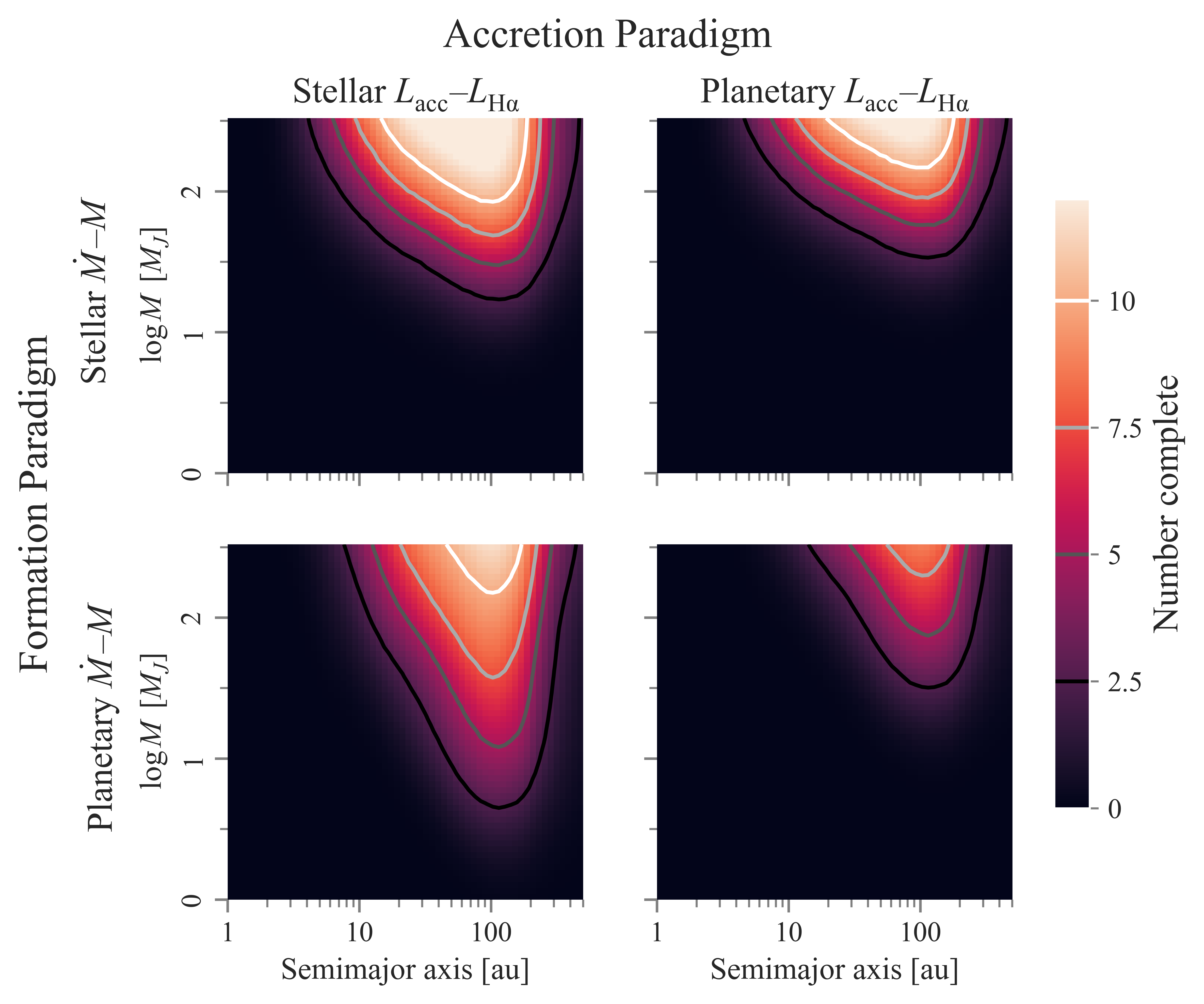
Figure 2: Completeness to accreting companions for the 14 stars surveyed by GAPlanetS as a function of semimajor axis [au] and mass $[M_{J}]$ for the four combinations of models. The color scale shows the depth of search, or the number of stars to which the survey is complete. The row dictates the $\dot{M}\textrm{--}M$ relation, with the top the stellar (B23) model and bottom the planetary (SH15) model. The column defines the $L_{\mathrm{H}\alpha}\textrm{--}L_{\mathrm{acc}}$ scaling, with the left the stellar (A17) and right the planetary (A21) scaling. Contours show completeness to 2.5, 5, 7.5, and 10 (out of 14) stars in the sample.

Current data suggest any of the four combinations of models shown here are possible. For instance, observations of Delorme 1 (AB)b suggest the presence of concentrated accretion columns (i.e., the stellar model), but a high disk mass indicative of formation by fragmentation (Ringqvist et al., 2023). The planetary-mass companion TWA27 B has a mass ratio $q\approx 0.2$ with its host star, implying the system formed more like a stellar binary, and its accretion properties are consistent with both the magnetospheric and planetary shock models (Marleau et al., 2024; Aoyama et al., 2024). Identifying the formation and accretion channels of a given object typically requires multiepoch, multiwavelength observations, which provide better measurements of $M$ and $\dot{M}$. While we limit this analysis to the H$\alpha$ results of GAPlanetS, future work will combine studies across wavelengths for stronger constraints.

5.1.1 Impact of eccentricity

To assess the effect of the assumed eccentricity distribution on sensitivity, we compare the completeness maps under fixed formation and accretion scaling relations, but with eccentricities from $P(e)\propto 2.1-2.2e$ versus circular orbits, $P(e)=\delta_{0,e}$. Figure 3 compares the results under the planetary formation and stellar accretion relation. The left panel shows the map assuming circular orbits, while the right panel plots the difference between the map allowing for eccentric orbits (the lower left panel of Figure 2) and the purely circular map. While the maps are qualitatively similar in shape, the map assuming circular orbits has more structure because not including eccentricity limits the spread of projected separation.

Eccentricity has the largest effect on detectability at wide semimajor axes, where circular-orbit companions are easier to detect. This is because eccentric companions are more likely to be projected beyond the edge of the image, decreasing detectability. At low semimajor axes, it is marginally easier to detect eccentric companions. Because the detectability threshold is highest at close separations, low semimajor axis planets are easier to detect when are eccentric and are, on average, farther from their host than their semimajor axis. The difference at low semimajor axes is more pronounced for individual stars; survey-averaged, the high-semimajor axis cutoff has a larger effect.

The difference in completeness between the eccentric and non-eccentric maps is slight, changing at most by 1.25 stars out of 14 (roughly $9\%$) at wide separations. Since demographics of giant planets suggest planets are more common at close separations (see Section 5.2.1 and references therein), the behavior toward small semimajor axes is likely more influential for detections.

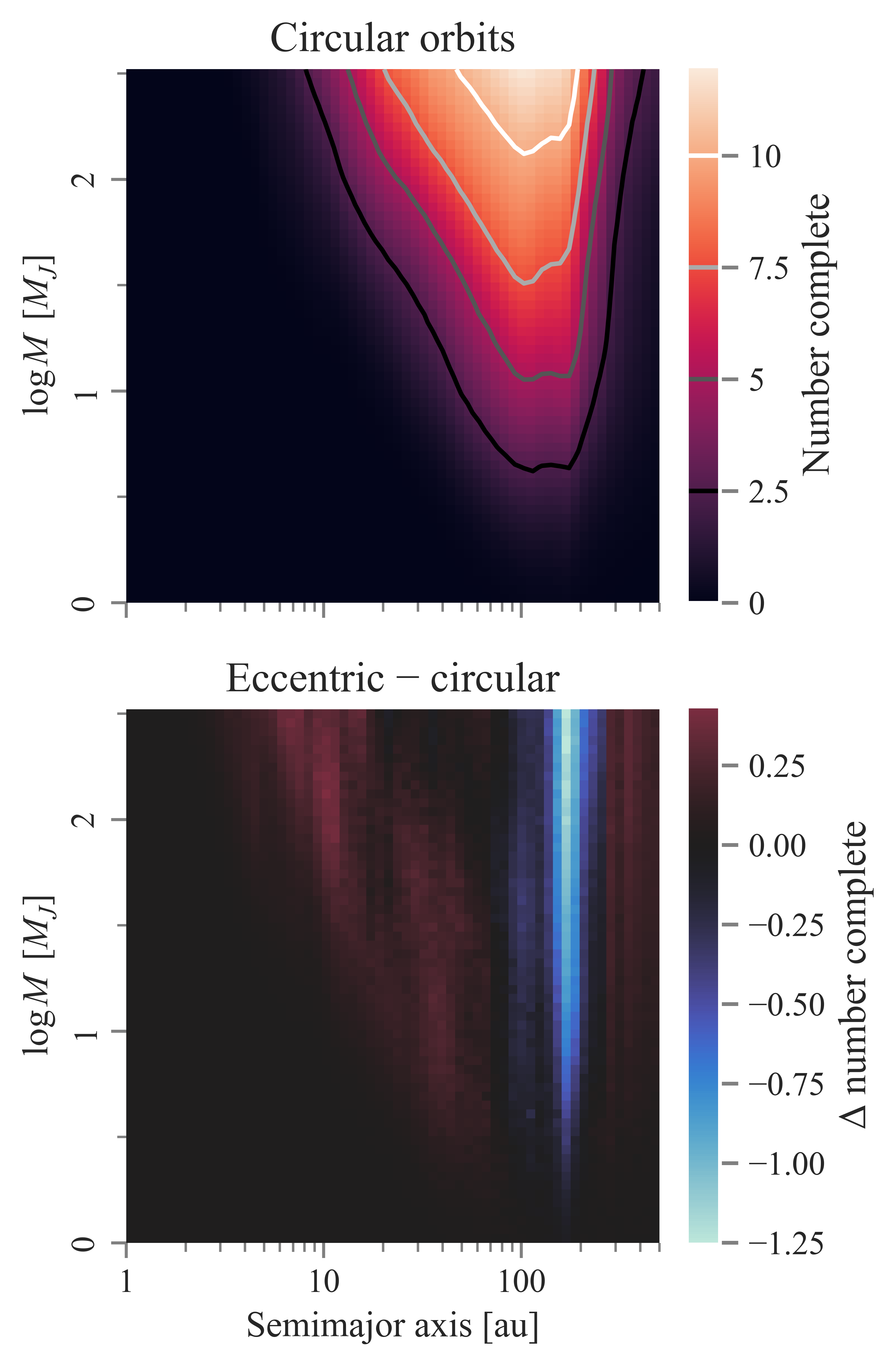
Figure 3: Top: GAPlanetS completeness to companions assuming circular orbits, $P(e)=\delta_{0,e}$, using the planetary $\dot{M}\textrm{--}M$ and stellar $L_{\mathrm{H}\alpha}\textrm{--}L_{\mathrm{acc}}$ scalings. The color scale and contours are as in Figure 2. Bottom: difference in survey sensitivity when assuming orbital eccentricities follow $P(e)\propto 2.1-2.2e$ (lower left panel of Figure 2) versus assuming circular orbits, $P(e)=\delta_{0,e}$. The colorbar shows the difference in the number of stars to which the survey is complete (out of 14); positive values indicate eccentric companions are easier to detect.

5.2 Constraints on protoplanet occurrence rate

To extend our completeness framework to constraints on protoplanet populations, we adopt the most conservative approach and do not rely on an assumption of the $\dot{M}\textrm{--}M$ relation, instead simulating $M\dot{M}$ as the physical parameter as covered in Section 2.2.3. Since we have precise constraints on separation but not semimajor axis, we also marginalize over semimajor axis to get completeness as a function of separation. When projecting into separation space, we assume a log-uniform prior in semimajor axis, $dN/da\propto a^{-1}$, as in Nielsen et al. (2019); Vigan et al. (2021). From the H$\alpha$ contrasts of the five GAPlanetS candidate protoplanet detections, we compute $M\dot{M}$ under both accretion scalings and and plot them over the completeness maps in Figure 4. For HD142527 B, which was observed in six epochs, we use the average separation and inferred $M\dot{M}$.

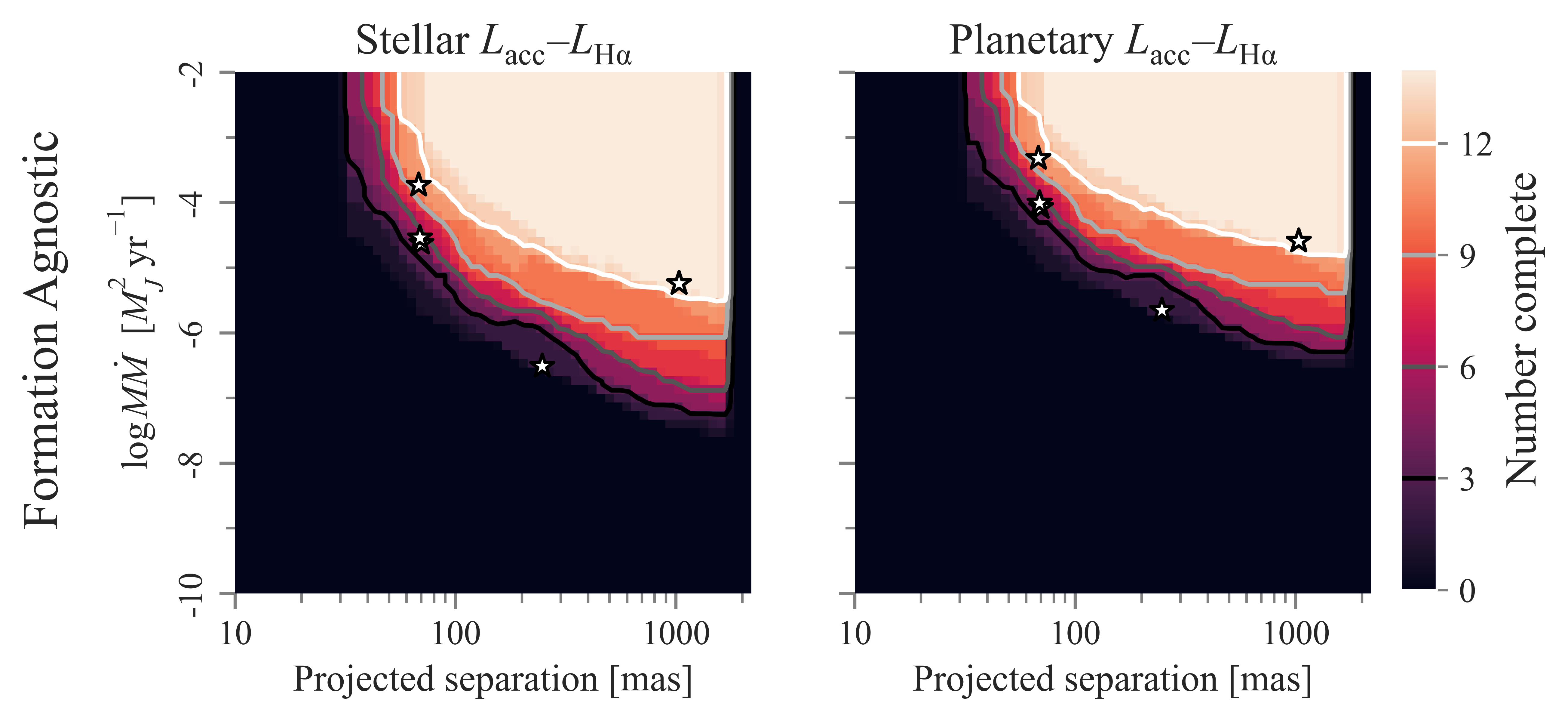
Figure 4: Survey-averaged completeness to accreting companions as a function of projected separation [mas] and $M\dot{M}$. The five GAPlanetS detections are overplotted as white stars. From left to right and top to bottom, these are CS Cha c, LkCa 15 b, HD142527 B, PDS70 c, and HD100453 B.

We then compute posteriors on the proportion of transitional disk stars with accreting companions. We do so for different subsets of the detected companions to analyze whether the estimate companion rate depends on either the companion or host star properties.

We consider accreting objects at separations 0.01–2.2 arcseconds and $-8\leq\log M\dot{M}/M_{J}^{2}\,\rm{yr}^{-1}\leq-2$. Although we performed simulations down to $\log M\dot{M}=-10\;M_{J}^{2}\,\rm{yr}^{-1}$, we exclude the lowest quarter of the parameter space to limit our analysis to regions with nonzero sensitivity (see Figure 4). We use log-uniform priors in $M\dot{M}$ and semimajor axis. Since we log-weighted semimajor axis when projecting the maps into separation, this becomes a uniform prior in separation. The total completeness to accreting objects, or overall search depth, is found by integrating the completeness map over the parameter space, weighted by the prior for each bin. Under these priors, GAPlanetS is complete to 7.8/14 stars under the stellar accretion relation and 6.3/14 stars under the planetary relation. Finally, we compute posteriors on accreting object occurrence rate using the Bayesian method described in Appendix A. In the analyses presented below, we exclude the candidate companions LkCa 15 b and CS Cha c to be more conservative about the accreting companion rate.

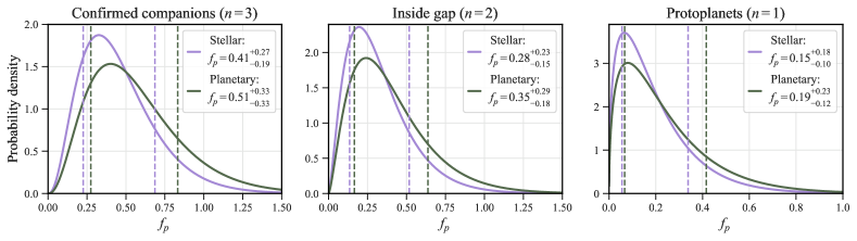
Figure 5: Posteriors on accreting object occurrence rate around stars hosting transitional disks, $f_{p}$, for different subsets of the GAPlanetS detections. In all, we compare the stellar (purple) and planetary (green) accretion scaling relations. The legends give the median and one-sigma uncertainties (16${}^{\textrm{th}}$ and 84${}^{\textrm{th}}$ percentiles), also marked by dashed lines. Left: posteriors on $f_{p}$ using the three confident detections. Center: posteriors on the rate of accreting companions inside disk gaps, excluding HD100453 B, which lies outside the gap. Right: posteriors on the accreting protoplanet rate, excluding the low-mass stars HD100453 B and HD142527 B.

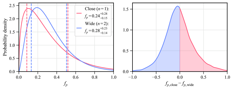
Figure 6: Left: posteriors on the occurrence rate of close ($<200$ mas, pink) versus wide ($\geq 200$ mas, blue) companions, assuming the stellar accretion scaling. As in Figure 5, the legend provides the one-sigma credible interval, also marked by dashed vertical lines. Here we consider the three confirmed companions, one of which is “close” and two of which are “wide.” Right: posterior on the difference in planet occurrence rate at close versus wide separations, $f_{p,\rm{close}}-f_{p,\rm{wide}}$; positive values (shaded in pink) indicate close companions are more common.

The left panel of Figure 5 shows the posterior distribution on the fraction of transitional disk systems hosting accreting objects in the parameter range 0.01–2.2 as and $-8\leq\log M\dot{M}/M_{J}^{2}\,\rm{yr}^{-1}\leq-2$, assuming the objects accrete by the stellar (purple) or planetary (green) accretion scaling relation. We label this quantity $f_{p}$, and note that it can be above unity (above 100%) if the average star hosts more than one accreting companion. Since planet-like accretors should be harder to detect (see Section 2.4 and Step C of Figure 1), if we assume the GAPlanetS detections accrete via the planetary model, we infer a higher underlying rate of accreting objects. Indeed, the median $f_{p}$ is 0.41 under the stellar model and 0.51 using the planetary. The maximum likelihood values are 0.32 and 0.39, respectively. However, the inferred companion rates are consistent to well within uncertainty. The one-sigma credible intervals (CIs) of $0.23-0.69$ (stellar model) and $0.28-0.83$ (planetary model) are consistent and broad, owing to small sample statistics.

The distributions in the leftmost panel of Figure 5 include two companions known to be low-mass stars: HD142527 B and HD100453 B. While HD142527 B is inside the transitional disk cavity, HD100453 B is an external perturber that is outside the main disk gap. Although HD142527 B is a star, its formation and accretion properties may be more similar to those of PDS70 c, and planets and brown dwarfs that formed inside disk gaps, than to HD100453 B and other stars. Non-embedded accreting companions, like HD100453 B and Delorme 1 (AB)b, may have distinct population properties. Since the properties of accreting companions in and outside transitional disk gaps may differ, we also compute the rate solely for the objects inside the gaps, shown in the center panel of Figure 5. Assuming the stellar (planetary) accretion model, the median and one-sigma CI on $f_{p}$ is $0.28^{+0.23}_{-0.15}$ ($0.35^{+0.29}_{-0.18}$), with maximum likelihood value $0.19$ ($0.24$).

We can also consider only the bona fide accreting protoplanet, PDS70 c. In the rightmost panel of Figure 5, we show posteriors on the rate of accreting protoplanets using this single detection. Supposing PDS70 c accretes via the magnetospheric (planetary) model, the median and one-sigma CI on $f_{p}$ is $0.15^{+0.18}_{-0.10}$ ($0.19^{+0.23}_{-0.12}$); with maximum likelihood $f_{p}=0.065$ ($0.080$).

Next, we look for correlations between planet and stellar properties and planet occurrence rate.

5.2.1 Impact of planet separation

Direct-imaging surveys for gas giants have demonstrated their rarity at wide ($\gtrsim 10$ au) separations, both by comparing the planet rate in bins of close and wide separation, and by inferring the power law index of the semimajor axis distribution (e.g. Nielsen et al. 2008; Wahhaj et al. 2013; Kasper et al. 2007; Chauvin et al. 2010; Vigan et al. 2012, 2017; Nielsen et al. 2019). We set the boundary between “close” and “wide” to be 200 mas ($\approx 20$ au, for the average stellar distance of $\approx$100 pc). With this division, we compute the posteriors for a transitional disk system hosting close versus wide accreting companions. For a more conservative estimate, we again exclude the candidate companions LkCa 15 b and CS Cha c, but include the low-mass stellar companions. The posteriors assuming the stellar accretion relation are shown in the left panel of Figure 6. The right panel shows the posterior on the difference in occurrence rate, $\Delta f_{p}=f_{p,\rm{close}}-f_{p,\rm{wide}}$, found by drawing values from the individual posteriors and subtracting them. We find no evidence of a difference in accreting companion rate based on separation; while the inferred $f_{p}$ for close companions has a lower median and longer tail, the uncertainties are so large that the posterior on $\Delta f_{p}$ is very nearly centered at 0. This inconclusive result is unsurprising given the small stellar sample size and few detections.

5.2.2 Impact of stellar mass

Searches for correlations between stellar mass and planet occurrence rate have found the rate increases with mass, both in radial velocity surveys (e.g. Wolthoff et al. 2022) and direct imaging (e.g. Bowler 2016; Lannier et al. 2016; Galicher et al. 2016; Meshkat et al. 2017). For the GPIES sample, Nielsen et al. (2019) both compares the rate in “low-mass” ($<1.5M_{\odot}$) and “high-mass” ($\geq 1.5M_{\odot}$) bins, and fits for a power-law dependence of $f_{p}$ with stellar mass. We adopt the same cutoff of $1.5M_{\odot}$ and compute the accreting companion occurrence rate around each subset of stars in the GAPlanetS sample. The masses for each survey star are given in Table 1. In the GAPlanetS case, the two stellar companions orbit “high-mass” stars (8/14, or 57% of the sample), while the lower mass protoplanets and protoplanet candidates orbit “low-mass” stars (6/14, or 43%, of the sample). This matches the intuition from selection effects. High-mass stars are intrinsically brighter: in the background-limited regime, the same achieved contrast means brighter, hence more massive, detectable objects. While we find the median inferred rate of accreting companions is slightly higher for the high-mass subsample, the rates for the low-mass and high-mass bins are consistent to well within uncertainty. The lack of evidence for a dependence of protoplanet frequency on stellar parameters is expected given our sample size.

6 Conclusion

Directly imaging protoplanets provides key insight into intermediate stages of planet and brown dwarf formation. With population inference, we can estimate the relative importance of different substellar formation pathways and the properties of the objects in each subpopulation. In this work, we present a method to quantify survey completeness to accreting protoplanets, and compute the first constraints on their population rate and whether it depends on companion or stellar properties. Presently, the code to compute completeness will be provided upon request to the corresponding author, and will be made publicly available in an upcoming Github release.

Determining accretion rate and mass limits for protoplanets requires assuming astrophysical models that govern the conversions between these physical properties and an object’s directly observable properties. We consider four main combinations of formation and accretion models in this work, though the technique is generalizable to any set of input relations. In particular, we compare two correlations between accreting objects’ masses and mass accretion rates: one corresponding a more “star-like”, or isolated, process, estimated from empirical observations of low-mass stars and brown dwarfs (Equation 2, B23); and one pertaining to a more “planet-like” process, computed from simulations of circumstellar disk fragmentation (Equation 3, SH15). For our constraints on protoplanet rate, we conservatively use a model that circumvents any assumption about the formation process, instead computing detectability as a function of $M\dot{M}$. The accretion scalings describe the proportion of total accretion luminosity that is emitted in the observable H$\alpha$ line, a proxy for the physics of the accretion flows. We use one correlation derived from observations of accreting stars, corresponding to magnetospheric accretion (Equation 5, A17), and one theoretical relation for a symmetric accretion shock on a planetary surface (Equation 6, A21).

We compute GAPlanetS’ completeness to companions that formed and accreted under each combination of models. Using the formation-agnostic model, we infer the frequency of accreting companions from GAPlanetS for various subsets of the detected objects. Using the three confirmed accreting companions, the median posterior occurrence rates are 41 and 51%, assuming the stellar or planetary accretion mechanism, respectively. For objects within transitional disk gaps, the median rates are 28% (35%) for the stellar (planetary) model. While one of these companions is a low-mass star, it differs from a field binary system because it is embedded in a disk. Specializing to the single certain protoplanet, the median posterior rates are 15% (19%). However, our small sample size contributes to broad credible intervals on the protoplanet occurrence rate. While we search for a dependence of the accreting companion rate on companion separation and stellar mass, our small number statistics and wide posteriors mean we do not conclude any correlation between companion rate and separation or stellar mass. Our current population analyses are suited to estimate rates under an assumed model, using subsets of the detections that we expect may have different properties. Currently, we do not have strong discriminating power on the population-level formation or accretion characteristics.

For tighter constraints on protoplanet rates, and to probe the population-level formation properties, we require a larger stellar sample size, lower uncertainties on confirmed companions’ parameters, and more detections. This method is generalizable to any combination of H$\alpha$ surveys. To incorporate additional survey stars, we require the instrument parameters and stellar properties needed to compute contrast (Equation 7), as well as the contrast curve for each star. Computing completeness and posteriors on accreting companion occurrence rate may then proceed as in Sections 4 and 5.2. Planned H$\alpha$ surveys for protoplanets such as the MaxProtoPlanetS survey (Close et al., 2020) will provide additional observations and, optimistically, detect new accreting objects. Alongside imaging more systems, both software and hardware developments will contribute to additional protoplanet detections.

An important avenue for increasing detections is improving the algorithms used to subtract the stellar point spread function, thus probing higher contrasts and at tighter separations (e.g. Bonse et al., 2024). Since planet frequency increases inward (Fernandes et al., 2019; Nielsen et al., 2019; Close, 2020), improved reductions from such algorithms may lead to new protoplanet candidates in GAPlanetS (and other surveys’) data. Instrument upgrades at Magellan (Males et al., 2024) and the VLT (Boccaletti et al., 2022) will likely have similar effects, potentially revealing new protoplanet candidates in these systems by achieving higher contrasts at tighter inner working angles (Close, 2020). Updated constraints on the accreting companion rate can then be found by rerunning the algorithm presented here.

Incorporating results from other accretion-tracing emission lines that may be more prominent in planets, such as He I or Pa$\beta$, is a promising avenue in terms of detections, although it may be more complicated in terms of interpretation. For instance, He I emission is also affected by winds (Thanathibodee et al., 2022; Erkal et al., 2022). Refining the relations used to link emission-line accretion diagnostics to the underlying accretion rates of substellar is a critical avenue for upcoming theoretical and observational work (e.g. Follette et al. 2024).

Constraints on protoplanet population properties using protoplanet surveys in multiple tracers, uniformly processed using improved PSF subtraction algorithms, will be the subject of future work. Applying our framework to compute survey completeness to protoplanets, upcoming protoplanet surveys can be fully capitalized on to bring us toward robust constraints on planet occurrence rate and formation mechanisms.

7 Acknowledgments

KBF and CP acknowledge funding from NSF-AST-2009816. G-DM acknowledges the support from the European Research Council under the Horizon 2020 Framework Program via the ERC Advanced Grant “Origins” (PI: Henning), Nr. 832428, and from the DFG priority program SPP 1992 “Exploring the Diversity of Extrasolar Planets” (MA 9185/1).

Appendix A Statistical frameworks

We infer the occurrence rate of protoplanets using a Bayesian approach, similar to the works of Vigan et al. (2012), Lannier et al. (2016), Nielsen et al. (2019), and Vigan et al. (2021). In a survey of $N$ transitional disk stellar systems, for each star we compute the detection probability as a function of $M\dot{M}$ and separation $s$, conditioned on astrophysical models $\Lambda$, $p_{\rm{det}}(M\dot{M},s\,|\,\Lambda)$. We denote by $f$ the true average number of accreting companions hosted by each system, with $M\dot{M}$ in the range $[M\dot{M}_{\rm{min}},M\dot{M}_{\rm{max}}]$ and separations $[s_{\rm{min}},s_{\rm{max}}]$. The fraction $f$ is assumed to be constant across the stellar sample; that is, we assume there is no correlation between stellar properties and companion rate. We then compute the average completeness to objects in that parameter range, $p$, weighted by priors on $M\dot{M}$ and separation:

$$p =\frac{1}{N}\sum_{i=1}^{N}\frac{1}{(M\dot{M}_{\rm{max}}-M\dot{M}_{\rm{min}})(s_{\rm{max}}-s_{\rm{min}})}\int_{M\dot{M}_{\rm{min}}}^{M\dot{M}_{\rm{max}}}\int_{s_{\rm{min}}}^{s_{\rm{max}}}p_{\rm{det},i}(M\dot{M},s)\pi(M\dot{M})\pi(s)d(M\dot{M})ds$$ (A1)

$$=\frac{1}{N}\sum_{i=1}^{N}p_{i}.$$ (A2)

We have dropped the conditional on models $\Lambda$ for simplicity but this dependence is implicit in all the following. In practice, these integrals are approximated on a discrete grid using a trapezoidal sum.

We suppose that planet occurrence follows a Poisson process with rate parameter $f$. The expected number of detections is then $\langle n_{\mathrm{det}}\rangle=fpN$. The probability of observing $n$ detections given the rate $f$, the likelihood $\mathcal{L}(n|f,N,p)$, is

$$\mathcal{L}(n|f,p,N)=\frac{e^{fpN}(fpN)^{n}}{n!}.$$ (A3)

Adopting a prior distribution on $f$, $\pi(f)$, Bayes’ theorem states the posterior probability of rate $f$ given the data $n,N$ is

$$P(f|n,p,N)=\frac{\mathcal{L}(n|f,p,N)\pi(f)}{\int_{0}^{1}\mathcal{L}(n|f,p,N)\pi(f)}df,$$ (A4)

where $P(n|p,N)=\int_{0}^{1}\mathcal{L}(n|f,p,N)\pi(f)df$ is the evidence. The posteriors presented in Section 5.2 are computed using a Jeffreys prior, $\pi(f)\propto f^{-1/2}$ for consistency with Nielsen et al. (2019).

To test the importance of the assumed prior, we also compute posteriors using a log-uniform prior, $\pi(f)\propto f^{-1}$, and a uniform prior $\pi(f)=1$. Because of the small sample size and correspondingly broad likelihood distribution, the posteriors are somewhat prior-driven. As shown in Figure 7, the log-uniform prior, which puts the most weight on low rates $f$, produces narrower posteriors with lower medians than the Jeffreys prior; using the uniform prior results in the widest posteriors with the highest inferred medians.

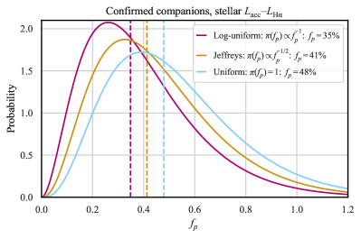
Figure 7: Comparison of posteriors on the companion rate under different prior assumptions: log-uniform (pink), Jeffreys (gold), and uniform (blue). These use the three confirmed companions and assume the stellar accretion scaling relation. The dashed vertical lines mark the median value for each.

References

- Adams Redai et al. (2023) Adams Redai, J. I., Follette, K. B., Wang, J., et al. 2023, AJ, 165, 57
- Alcalá et al. (2014) Alcalá, J. M., Natta, A., Manara, C. F., et al. 2014, A&A, 561, A2
- Alcalá et al. (2017) Alcalá, J. M., Manara, C. F., Natta, A., et al. 2017, A&A, 600, A20
- Almendros-Abad et al. (2024) Almendros-Abad, V., Manara, C. F., Testi, L., et al. 2024, A&A, 685, A118
- Aoyama et al. (2022) Aoyama, Y., Herczeg, G. J., Beck, T., Hashimoto, J., & Zhou, Y. 2022, Testing models of accretion onto the Young Planetary System PDS 70, HST Proposal. Cycle 30, ID. #17127
- Aoyama et al. (2018) Aoyama, Y., Ikoma, M., & Tanigawa, T. 2018, ApJ, 866, 84
- Aoyama et al. (2024) Aoyama, Y., Marleau, G.-D., & Hashimoto, J. 2024, arXiv e-prints, arXiv:2407.15922
- Aoyama et al. (2021) Aoyama, Y., Marleau, G.-D., Ikoma, M., & Mordasini, C. 2021, ApJ, 917, L30
- Aoyama et al. (2020) Aoyama, Y., Marleau, G.-D., Mordasini, C., & Ikoma, M. 2020, arXiv e-prints, arXiv:2011.06608
- Balmer et al. (2022) Balmer, W. O., Follette, K. B., Close, L. M., et al. 2022, AJ, 164, 29
- Betti et al. (2022) Betti, S. K., Follette, K. B., Ward-Duong, K., et al. 2022, ApJ, 935, L18
- Betti et al. (2023) Betti, S. K., Follette, K. B., Ward-Duong, K., et al. 2023, AJ, 166, 262
- Biddle et al. (2024) Biddle, L. I., Bowler, B. P., Zhou, Y., Franson, K., & Zhang, Z. 2024, AJ, 167, 172
- Biller et al. (2007) Biller, B. A., Close, L. M., Masciadri, E., et al. 2007, ApJS, 173, 143
- Blunt et al. (2020) Blunt, S., Wang, J. J., Angelo, I., et al. 2020, AJ, 159, 89
- Boccaletti et al. (2022) Boccaletti, A., Chauvin, G., Wildi, F., et al. 2022, in Society of Photo-Optical Instrumentation Engineers (SPIE) Conference Series, Vol. 12184, Ground-based and Airborne Instrumentation for Astronomy IX, ed. C. J. Evans, J. J. Bryant, & K. Motohara, 121841S
- Bonse et al. (2023) Bonse, M. J., Garvin, E. O., Gebhard, T. D., et al. 2023, AJ, 166, 71
- Bonse et al. (2024) Bonse, M. J., Gebhard, T. D., Dannert, F. A., et al. 2024, arXiv e-prints, arXiv:2406.01809
- Bowler (2016) Bowler, B. P. 2016, PASP, 128, 102001
- Bowler et al. (2020) Bowler, B. P., Blunt, S. C., & Nielsen, E. L. 2020, AJ, 159, 63
- Bowler et al. (2015) Bowler, B. P., Liu, M. C., Shkolnik, E. L., & Tamura, M. 2015, ApJS, 216, 7
- Butler et al. (2006) Butler, R. P., et al. 2006, Astrophys. J., 646, 505
- Calvet & Gullbring (1998) Calvet, N., & Gullbring, E. 1998, ApJ, 509, 802
- Chauvin et al. (2010) Chauvin, G., Lagrange, A. M., Bonavita, M., et al. 2010, A&A, 509, A52
- Chilcote et al. (2022) Chilcote, J., Konopacky, Q., Fitzsimmons, J., et al. 2022, in Society of Photo-Optical Instrumentation Engineers (SPIE) Conference Series, Vol. 12184, Ground-based and Airborne Instrumentation for Astronomy IX, ed. C. J. Evans, J. J. Bryant, & K. Motohara, 121841T
- Close (2020) Close, L. M. 2020, AJ, 160, 221
- Close et al. (2013) Close, L. M., Males, J. R., Morzinski, K., et al. 2013, ApJ, 774, 94
- Close et al. (2020) Close, L. M., Males, J., Long, J. D., et al. 2020, in Society of Photo-Optical Instrumentation Engineers (SPIE) Conference Series, Vol. 11448, Adaptive Optics Systems VII, ed. L. Schreiber, D. Schmidt, & E. Vernet, 114480U
- Currie (2024) Currie, T. 2024, Research Notes of the American Astronomical Society, 8, 146
- Currie et al. (2019) Currie, T., Marois, C., Cieza, L., et al. 2019, ApJ, 877, L3
- Currie et al. (2022) Currie, T., Lawson, K., Schneider, G., et al. 2022, Nature Astronomy, 6, 751
- Do Ó et al. (2023) Do Ó, C. R., O’Neil, K. K., Konopacky, Q. M., et al. 2023, AJ, 166, 48
- Dodson-Robinson & Salyk (2011) Dodson-Robinson, S. E., & Salyk, C. 2011, ApJ, 738, 131
- Duchêne & Kraus (2013) Duchêne, G., & Kraus, A. 2013, ARA&A, 51, 269
- Dullemond et al. (2006) Dullemond, C. P., Natta, A., & Testi, L. 2006, ApJ, 645, L69
- Emsenhuber et al. (2021) Emsenhuber, A., Mordasini, C., Burn, R., et al. 2021, A&A, 656, A69
- Erkal et al. (2022) Erkal, J., Manara, C. F., Schneider, P. C., et al. 2022, A&A, 666, A188
- Fernandes et al. (2019) Fernandes, R. B., Mulders, G. D., Pascucci, I., Mordasini, C., & Emsenhuber, A. 2019, ApJ, 874, 81
- Fiorellino et al. (2022) Fiorellino, E., Tychoniec, Ł., Manara, C. F., et al. 2022, ApJ, 937, L9
- Follette et al. (2017) Follette, K. B., Rameau, J., Dong, R., et al. 2017, Astronomical Journal, 153, 264
- Follette et al. (2023) Follette, K. B., Close, L. M., Males, J. R., et al. 2023, AJ, 165, 225
- Follette et al. (2024) Follette, K. B., Aoyama, Y., Bary, J. S., et al. 2024, Bridging Accretion Mechanisms from Stars to Planets with NIR Diagnostics, JWST Proposal. Cycle 3, ID. #6361
- Forgan & Rice (2013) Forgan, D., & Rice, K. 2013, MNRAS, 432, 3168
- Fu et al. (2023) Fu, Z., Huang, S., & Yu, C. 2023, ApJ, 945, 165
- Galicher et al. (2016) Galicher, R., Marois, C., Macintosh, B., et al. 2016, A&A, 594, A63
- Gratton et al. (2019) Gratton, R., Ligi, R., Sissa, E., et al. 2019, A&A, 623, A140
- Haffert et al. (2019) Haffert, S. Y., Bohn, A. J., de Boer, J., et al. 2019, Nature Astronomy, 3, 749
- Haffert et al. (2021) Haffert, S. Y., Males, J. R., Close, L., et al. 2021, in Society of Photo-Optical Instrumentation Engineers (SPIE) Conference Series, Vol. 11823, Techniques and Instrumentation for Detection of Exoplanets X, ed. S. B. Shaklan & G. J. Ruane, 1182306
- Hammond et al. (2023) Hammond, I., Christiaens, V., Price, D. J., et al. 2023, MNRAS, 522, L51
- Hartmann et al. (2016) Hartmann, L., Herczeg, G., & Calvet, N. 2016, ARA&A, 54, 135
- Huélamo et al. (2022) Huélamo, N., Chauvin, G., Mendigutía, I., et al. 2022, A&A, 668, A138
- Kasper et al. (2007) Kasper, M., Apai, D., Janson, M., & Brandner, W. 2007, A&A, 472, 321
- Keppler et al. (2018) Keppler, M., Benisty, M., Müller, A., et al. 2018, A&A, 617, A44
- Kipping (2013) Kipping, D. M. 2013, MNRAS, 434, L51
- Koenigl (1991) Koenigl, A. 1991, ApJ, 370, L39
- Kraus & Ireland (2012) Kraus, A. L., & Ireland, M. J. 2012, ApJ, 745, 5
- Lambrechts & Johansen (2012) Lambrechts, M., & Johansen, A. 2012, A&A, 544, A32
- Lannier et al. (2016) Lannier, J., Delorme, P., Lagrange, A. M., et al. 2016, A&A, 596, A83
- Lin & Papaloizou (1993) Lin, D. N. C., & Papaloizou, J. C. B. 1993, in Protostars and Planets III, ed. E. H. Levy & J. I. Lunine, 749
- Males (2013) Males, J. R. 2013, PhD thesis, University of Arizona
- Males et al. (2024) Males, J. R., Close, L. M., Haffert, S. Y., et al. 2024, arXiv e-prints, arXiv:2407.13007
- Manara et al. (2015) Manara, C. F., Testi, L., Natta, A., & Alcalá, J. M. 2015, A&A, 579, A66
- Manara et al. (2016) Manara, C. F., Rosotti, G., Testi, L., et al. 2016, A&A, 591, L3
- Manara et al. (2017) Manara, C. F., Testi, L., Herczeg, G. J., et al. 2017, A&A, 604, A127
- Marleau et al. (2024) Marleau, G.-D., Aoyama, Y., Hashimoto, J., & Zhou, Y. 2024, ApJ, 964, 70
- Marleau et al. (2023) Marleau, G.-D., Kuiper, R., Béthune, W., & Mordasini, C. 2023, ApJ, 952, 89
- Mawet et al. (2014) Mawet, D., Milli, J., Wahhaj, Z., et al. 2014, ApJ, 792, 97
- Meshkat et al. (2017) Meshkat, T., Mawet, D., Bryan, M. L., et al. 2017, AJ, 154, 245
- Mordasini et al. (2012) Mordasini, C., Alibert, Y., Georgy, C., et al. 2012, A&A, 547, A112
- Morzinski et al. (2014) Morzinski, K. M., Close, L. M., Males, J. R., et al. 2014, in Society of Photo-Optical Instrumentation Engineers (SPIE) Conference Series, Vol. 9148, Adaptive Optics Systems IV, ed. E. Marchetti, L. M. Close, & J.-P. Vran, 914804
- Morzinski et al. (2016) Morzinski, K. M., Close, L. M., Males, J. R., et al. 2016, in Society of Photo-Optical Instrumentation Engineers (SPIE) Conference Series, Vol. 9909, Adaptive Optics Systems V, ed. E. Marchetti, L. M. Close, & J.-P. Véran, 990901
- Muzerolle et al. (2005) Muzerolle, J., Luhman, K. L., Briceño, C., Hartmann, L., & Calvet, N. 2005, ApJ, 625, 906
- Natta et al. (2006) Natta, A., Testi, L., & Randich, S. 2006, A&A, 452, 245
- Nielsen et al. (2008) Nielsen, E. L., Close, L. M., Biller, B. A., Masciadri, E., & Lenzen, R. 2008, ApJ, 674, 466
- Nielsen et al. (2019) Nielsen, E. L., De Rosa, R. J., Macintosh, B., et al. 2019, AJ, 158, 13
- Price et al. (2018) Price, D. J., Cuello, N., Pinte, C., et al. 2018, MNRAS, 477, 1270
- Rafikov (2017) Rafikov, R. R. 2017, ApJ, 837, 163
- Rameau et al. (2017) Rameau, J., Follette, K. B., Pueyo, L., et al. 2017, AJ, 153, 244
- Reggiani et al. (2014) Reggiani, M., Quanz, S. P., Meyer, M. R., et al. 2014, ApJ, 792, L23
- Reipurth & Clarke (2001) Reipurth, B., & Clarke, C. 2001, AJ, 122, 432
- Ringqvist et al. (2023) Ringqvist, S. C., Viswanath, G., Aoyama, Y., et al. 2023, A&A, 669, L12
- Safronov (1972) Safronov, V. S. 1972, Evolution of the protoplanetary cloud and formation of the earth and planets. (Keter Publishing House)
- Sallum et al. (2015) Sallum, S., Follette, K. B., Eisner, J. A., et al. 2015, Nature, 527, 342
- Shibaike & Mordasini (2024) Shibaike, Y., & Mordasini, C. 2024, A&A, 687, A166
- Somigliana et al. (2022) Somigliana, A., Toci, C., Rosotti, G., et al. 2022, MNRAS, 514, 5927
- Stamatellos & Herczeg (2015) Stamatellos, D., & Herczeg, G. J. 2015, MNRAS, 449, 3432
- Stamatellos & Whitworth (2009) Stamatellos, D., & Whitworth, A. P. 2009, MNRAS, 392, 413
- Tanigawa et al. (2012) Tanigawa, T., Ohtsuki, K., & Machida, M. N. 2012, ApJ, 747, 47
- Thanathibodee et al. (2022) Thanathibodee, T., Calvet, N., Hernández, J., Maucó, K., & Briceño, C. 2022, AJ, 163, 74
- Toomre (1964) Toomre, A. 1964, ApJ, 139, 1217
- Vigan et al. (2012) Vigan, A., Patience, J., Marois, C., et al. 2012, A&A, 544, A9
- Vigan et al. (2017) Vigan, A., Bonavita, M., Biller, B., et al. 2017, A&A, 603, A3
- Vigan et al. (2021) Vigan, A., Fontanive, C., Meyer, M., et al. 2021, A&A, 651, A72
- Wahhaj et al. (2013) Wahhaj, Z., Liu, M. C., Nielsen, E. L., et al. 2013, ApJ, 773, 179
- Wahhaj et al. (2024) Wahhaj, Z., Benisty, M., Ginski, C., et al. 2024, A&A, 687, A257
- Wang et al. (2015) Wang, J. J., Ruffio, J.-B., De Rosa, R. J., et al. 2015, pyKLIP: PSF Subtraction for Exoplanets and Disks, Astrophysics Source Code Library, record ascl:1506.001
- Wang et al. (2021) Wang, J. J., Vigan, A., Lacour, S., et al. 2021, AJ, 161, 148
- Wolthoff et al. (2022) Wolthoff, V., Reffert, S., Quirrenbach, A., et al. 2022, A&A, 661, A63
- Zhou et al. (2021a) Zhou, Y., Bae, J., Bowler, B., et al. 2021a, A Search for Accreting Protoplanets within Transition Disk Gaps, HST Proposal. Cycle 29, ID. #16651
- Zhou et al. (2021b) Zhou, Y., Bowler, B. P., Wagner, K. R., et al. 2021b, AJ, 161, 244
- Zhou et al. (2022) Zhou, Y., Sanghi, A., Bowler, B. P., et al. 2022, ApJ, 934, L13
- Zurlo et al. (2020) Zurlo, A., Cugno, G., Montesinos, M., et al. 2020, A&A, 633, A119