Linear response in planar Hall and thermal Hall setups for Rarita-Schwinger-Weyl semimetals

Abstract

We investigate the nature of the linear-response tensors in planar Hall and planar thermal Hall setups, where we subject a Rarita-Schwinger-Weyl (RSW) semimetal to the combined influence of an electric field $\mathbf{E}$ (and/or temperature gradient $\nabla_{\mathbf{r}}T$) and a weak (i.e., non-quantizing) magnetic field $\mathbf{B}$. For computing the in-plane transport components, we have added an elastic deformation which gives rise to a chirality-dependent effective magnetic field $\mathbf{B}^{\text{tot}}=\mathbf{B}+\chi\,\mathbf{B}_{5}$, where $\chi$ is the chirality of an RSW node. We have included the effects of orbital magnetic moment (OMM), in conjunction with the Berry curvature (BC), both of which appear as a consequence of nontrivial topology of the bandstructure. Due to the presence of four bands, RSW semimetals provide a richer structure for obtaining the linear-response coefficients, compared to the Weyl semimetals. In particular, we have found that the OMM-contributed terms may oppose or add up to the BC-only parts, depending on which band we are considering. We have also considered the response arising from internode scatterings. Last, but not the least, we have determined the out-of-plane response comprising the intrinsic anomalous Hall and the Lorentz-force-contributed currents, whose nature corroborates the findings of some recent experimental results.

I Introduction

There has been an overwhelming amount of research activities involving the transport characteristics of semimetals, which are materials containing band-crossing points in the Brillouin zone (BZ) near the Fermi level, determined and protected by some symmetry. The terminology of “semimetals” originates from the fact that the density-of-states go exactly to zero at these nodal points, showcasing a feature which is neither like insulators (as there is no gap) nor like conventional metals — it lies somewhere in the middle of the two opposites. The simplest and the most well-known three-dimensional (3d) example is the Weyl semimetal (WSM) [1, 2], which harbours an isotropic linear-in-momentum dispersion in the vicinity of twofold band-crossings. The most straightforward generalization of the WSM is a semimetal with multifold band-crossings, where each band exhibits an isotropic linear dispersion. The low-energy effective Hamiltonian of a system, with $(2\,\varsigma+1)$ bands touching at a point, can be expressed as $\sim\mathbf{k}\cdot\bm{\mathcal{S}}$, where $\bm{\mathcal{S}}$ represents the three components of the angular momentum operator in the spin-$\varsigma$ representation of the SO(3) group. This gives rise to emergent quasiparticles carrying pseudospin values equal to $\varsigma$. We use the nomenclature “pseudospin” in order to clearly distinguish this quantum number from the relativistic spin (arising from the spacetime Lorentz invariance). Examples of multiband semimetals, featuring $\varsigma>1/2$, include the pseudospin-3/2 Rarita-Schwinger-Weyl (RSW) semimetals [3, 4, 5, 6, 7, 8, 9, 10, 11, 12, 13, 14, 15] with fourfold band-crossings.

In the realm of high-energy physics, the Rarita-Schwinger (RS) equation describes the field equation for elementary particles carrying the relativistic spin of 3/2, postulated in various supergravity models [16]. However, they neither appear in the standard model, nor has been detected experimentally. On the other hand, in nonrelativistic condensed matter systems, we find that there are 230 space groups, paving the way for the emergence of a rich variety of unconventional excitations. In fact, for each one of these space groups, there exist pseudospin quantum numbers dictated by the irreducible representations of the little group of lattice symmetries at the high-symmetry points (in the BZ) [3]. The RSW semimetals represent one such possibility, mimicking the relativistic spin-3/2 fermions, because of the quasiparticles carrying pseudospin-3/2. Their nomenclature thus mirrors the elusive high-energy RS fermions.

To investigate the so-called topological properties of a solid state material, we consider the BZ as a closed manifold. When a nodal-point semimetal is said to possess a BZ endowed with a nontrivial topology, the nodes represent zero-dimensional topological defects, which thus carry nontrivial topological charges in the form of Berry curvature (BC) monopoles [17, 18]. The sign of the monopole charge gives us the chirality $\chi$ of the node, leading to the nomenclature of right-moving and left-moving chiral quasiparticles, corresponding to $\chi=1$ and $\chi=-1$, respectively. The nodes are constrained to appear in pairs, with each pair having opposite chiralities, which is easily explained by invoking the Nielson-Ninomiya theorem [19]. We will adopt the convention that $\chi$ refers to the sign of the monopole charges (or, equivalently, the Chern numbers) of the negative-energy bands (i.e., the valence bands) — thus a positive(negative) sign indicates that the node acts as a source(sink) for the flux lines of the BC vector field. For a given band, the monopole charge is obtained by integrating the BC flux over a closed two-dimensional (2d) surface enclosing the nodal point. The combined Chern number of all the bands corresponds to the wrapping of a generalized Bloch sphere $S^{n}$ (generalized to an $n$-level quantum system), representing the manifold of the quantum states. On the other hand, if we project on to the bands of a given pseudospin value (thus giving us a two-level system), the Chern number represents a wrapping number of the map from the 2d closed surface (topologically equivalent to $S^{2}$) to the Bloch sphere ($S^{2}$), given by the elements of the second homotopy group $\Pi_{2}(S^{2})=\mathbb{Z}$. The WSM belongs to this category, with Chern numbers $\pm 1$. This explains why the monopole charges, represnting point defects, can be interpreted as Chern numbers as well.

Analogous to the WSMs, the RSW nodes carry nonzero values of the BC monopoles. The four bands at a single RSW node have Chern numbers $\pm 1$ and $\pm 3$, which indicates a net monopole charge of magnitude 4. The indications of the existence of RSW quasiparticles have been linked to the large values of the topological charges detected in a range of materials, such as $\mathrm{CoSi}$ [20], $\mathrm{RhSi}$ [21], $\mathrm{AlPt}$ [22], and $\mathrm{PdBiSe}$ [23]. The chiral anomaly, a signature property of the relativistic Weyl fermions, explained by Adler-Bell-Jackiw [24, 25], continue to hold in the nonrelativistic settings involving WSMs [26]. In the context of the condensed matter systems, the anomaly refers to the phenomenon of charge pumping from one node to its conjugate, under the combined influence of applied electric ($\mathbf{E}$) and magnetic ($\mathbf{B}$) fields, with a rate $\propto\mathbf{E}\cdot\mathbf{B}$. Thus, for $\mathbf{E}\cdot\mathbf{B}\neq 0$, the number of quasiparticless of each chirality is not independently conserved in the vicinity of an individual node, and is known as the electrical chiral anomaly (ECA). Nevertheless, the net chiral charge for the conjugate pairs of nodes in the entire BZ yields zero, thus conserving the total electric charge. An analogous imbalance in chiral charge can be caused by adding (or replacing the external electric field by) an external temperature gradient $\mathbf{\nabla}_{\mathbf{r}}T$, manifesting itself as the thermal chiral anomaly (TCA), being proportional to $\nabla_{\mathbf{r}}T\cdot\mathbf{B}$ [27]. A nonzero $\nabla_{\mathbf{r}}T\cdot\mathbf{B}\neq 0$ also results in an imbalance in chiral energy (i.e., the energy carried by the quasiparticles of same chirality), which is sometimes referred to as the gravitational chiral anomaly (GCA) [28, 29, 27], and it contributes to the energy current.

In this paper, we consider planar Hall setups consisting of $\mathbf{E}$ (and/or $\nabla_{\mathbf{r}}T$) and $\mathbf{B}$ fields [cf. Fig. 1] and involving RSW semimetals. We choose $\mathbf{E}$ and $\mathbf{B}$ to lie in the $xy$-plane, with $\mathbf{E}$ (or $\nabla_{\mathbf{r}}T$) applied along the $x$-axis. In other words, $\mathbf{B}=B\left(\cos\theta,\sin\theta,0\right)$ (where $B\equiv|\mathbf{B}|$), such that $\theta\neq\pi/2\text{ or }3\,\pi/2$ in general. In the linear response regime (with respect to $\mathbf{E}$ and $\nabla_{\mathbf{r}}T$), the node-dependent transport coefficients, relating the electric current to $\mathbf{E}$ and $\nabla_{\mathbf{r}}T$, are the magnetoelectric conductivity tensor ($\sigma^{\chi}$) and the magnetothermoelectric conductivity tensor ($\alpha^{\chi}$), respectively. A third response tensor, which we denote by $\ell^{\chi}$, is the linear response tensor relating the heat current to the temperature gradient at a vanishing electric field. Since $\ell^{\chi}$ contributes to the magnetothermal conductivity tensor $\kappa^{\chi}$, we will often loosely refer to $\ell^{\chi}$ itself as the magnetothermal coefficient. The longitudinal components, $\sigma_{xx}^{\chi}$ and $\alpha^{\chi}_{xx}$, are known as the longitudinal magnetoconductivity (LMC) and the longitudinal thermoelectric coefficient (LTEC), respectively. The transverse components, $\sigma_{yx}^{\chi}$ and $\alpha^{\chi}_{yx}$, are referred to as the planar Hall conductivity (PHC) and the transverse thermoelectric coefficient (TTEC), respectively. In recent times, there has been a surge of theoretical and experimental efforts to investigate various aspects of these response tensors [30, 31, 32, 33, 34, 27, 35, 36, 37, 38, 39, 40, 41, 42, 43, 44, 45, 46, 15, 47].

All the linear-response coefficients invariably contain the information about nontrivial band topology via the inclusion of the BC. In addition, the orbital magnetic moment (OMM) [48, 49], which is another artifact of a nontrivial topology in the bandstructures, also affects the behaviour of the response tensors [42, 43, 47]. Hence, in this paper, we include the effects of both the BC and the OMM, which constitutes a complete description conveying the role of topology. It is worth mentioning here that complementary evidence of nontrivial topology in bandstructures, extensively explored in the literature, include intrinsic anomalous Hall effect [50, 51, 52], magneto-optical conductivity when Landau levels are relevant [53, 54, 55], Magnus Hall effect [56, 57, 12], circular dichroism [10, 58], circular photogalvanic effect [59, 60, 61, 62], and transmission of quasiparticles across potential barriers/wells [63, 64, 65, 13].

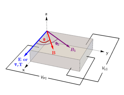
Figure 1: Schematics of the planar Hall (or planar thermal Hall) setup, where an RSW is subjected to a static electric field $E\,{\mathbf{\hat{x}}}$ (or temperature gradient $\partial_{x}T\,{\mathbf{\hat{x}}}$). An external magnetic field $\mathbf{B}$ is applied at an angle $\theta$ with respect to the electric field (temperature gradient). Additionally, the semimetallic slab is subjected to a mechanical strain, whose effect is captured via an artificial pseudomagnetic field $\mathbf{B}_{5}$, making an angle $\theta_{5}$ with the $x$-axis. The in-plane voltage generated parallel and perpendicular to $E\,{\mathbf{\hat{x}}}$ (or $\partial_{x}T\,{\mathbf{\hat{x}}}$) are indicated by $V_{\rm LC}$ and $V_{\rm PH}$, respectively. The subscripts indicate their association with the longitudinal and Hall components of the resulting currents.

In addition to the action of the externally-applied magnetic field, we consider the case when the semimetal is subjected to a mechanical strain, thus undergoing elastic deformations. The effects of these deformations on the chiral quasiparticles can be modelled as pseudogauge fields [66, 67, 68, 69, 70, 71, 72, 43], with the matter-gauge-field coupling constant being proportional to $\chi$ [69, 70, 71, 73, 74, 43]. Due to the chiral nature of the coupling between the emergent vector fields and the itinerant fermionic particles, it provides a platform to study the interactions of matter with axial vector fields in three dimensions. This property differs from the case of the actual electromagnetic fields, where the coupling constant is independent of $\chi$. It has been shown theoretically that a uniform pseudomagnetic field $\mathbf{B}_{5}$ can be generated when a semimetallic nanowire is put under torsion [71]. Some direct experimental evidence for the generation of such pseudoomagnetic fields is also available [75].

The paper is organized as follows. In Sec. II, we outline the form of the low-energy effective Hamiltonian in the vicinity of an RSW node, and the resulting expressions for the BC and OMM. In Sec. A, we review the steps to compute the conductivity tensor using the semiclassical Boltzmann formalism, without considering internode scattering. Secs. III andIV are devoted to demonstrating the explicit expressions for the longitudinal and transverse components of $\sigma^{\chi}$, $\alpha^{\chi}$, and $\ell^{\chi}$, respectively. The last subsection of Sec. III also illustrates their behaviour in some relevant parameter regimes. In Sec. V, we discuss the outcome of the inclusion of internode scatterings. Here, we also consider the effects of the so-called Lorentz force parts, which show up in the out-of-plane components of the response coefficients, and compare it with some recent experimental observations. Finally, we conclude with a summary and outlook in Sec. VI. The appendices are devoted to elaborating on some the details of the intermediate steps, necessary to derive the final expressions shown in the main text. In all our expressions, we resort to using the natural units, which implies that the reduced Planck’s constant ($\hbar$), the speed of light ($c$), and the Boltzmann constant ($k_{B}$) are set to unity.

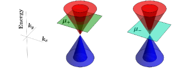
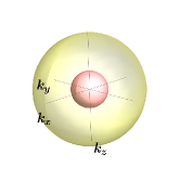
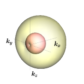
Figure 2: (a) The dispersion of a pair of conjugate RSW nodes, against the $k_{x}k_{y}$-plane. The chemical potentials, $\mu_{+}$ and $\mu_{-}$, cut the conduction bands with chiralitties $+1$ and $-1$, respectively. (b) Schematics of the Fermi surfaces at the node with chirality $+1$, without and with the OMM-correction for the effective energy dispersion. Here, we have taken the net effective magnetic field to be directed purely along the $x$-axis.

II Model

With the help of group-theoretic symmetry analysis and first principles calculations, it has been shown that seven space groups may host fourfold band-crossing points [3] at high symmetry points of the BZ. Nearly 40 candidate materials have also been identified that can host the resulting RSW quasiparticles. The usual method of linearizing the $\mathbf{k}\cdot\mathbf{p}$ Hamiltonian about such a degeneracy point provides us with the low-energy effective continuum Hamiltonian, valid in the vicinity of the node. The explicit form of this Hamiltonian, for a single node with chirality $\chi$, is given by

$$\mathcal{H}(\mathbf{k})=v_{0}\left(k_{x}\,{\mathcal{J}}_{x}+k_{y}\,{\mathcal{J}}_{y}+\chi\,k_{z}\,{\mathcal{J}}_{z}\right),$$ (1)

where $\bm{\mathcal{J}}=\{{\mathcal{J}}_{x},\,{\mathcal{J}}_{y},\,{\mathcal{J}}_{z}\}$ represents the vector operator whose three components comprise the the angular momentum operators in the spin-$3/2$ representation of the SO(3) group. We choose the commonly-used representation where

$${\mathcal{J}}_{x}=\begin{pmatrix}0&\frac{\sqrt{3}}{2}&0&0\\ \frac{\sqrt{3}}{2}&0&1&0\\ 0&1&0&\frac{\sqrt{3}}{2}\\ 0&0&\frac{\sqrt{3}}{2}&0\end{pmatrix},\quad{\mathcal{J}}_{y}=\begin{pmatrix}0&\frac{-i\,\sqrt{3}}{2}&0&0\\ \frac{i\,\sqrt{3}}{2}&0&-i&0\\ 0&i&0&\frac{-i\,\sqrt{3}}{2}\\ 0&0&\frac{i\,\sqrt{3}}{2}&0\end{pmatrix},\quad{\mathcal{J}}_{z}=\begin{pmatrix}\frac{3}{2}&0&0&0\\ 0&\frac{1}{2}&0&0\\ 0&0&-\frac{1}{2}&0\\ 0&0&0&-\frac{3}{2}\end{pmatrix}.$$ (2)

Our convention is such that the pair of conjugate nodes are separated along the $k_{z}$-direction. The energy eigenvalues are found to be

$$\varepsilon_{s}(k)=s\,v_{0}\,k\,,\quad s\in\left\{\pm\frac{1}{2},\pm\frac{3}{2}\right\},$$ (3)

where $k=\sqrt{k_{x}^{2}+k_{y}^{2}+k_{z}^{2}}$. Hence, each of four bands has an isotropic linear-in-momentum dispersion [cf. Fig. 2(a)]. The signs of “$+$” and “$-$” give us the dispersion relations for the conduction and valence bands, respectively. The corresponding group velocities of the quasiparticles are given by

$$\bm{v}_{s}(\mathbf{k}) =\nabla_{\mathbf{k}}\varepsilon_{s}(\mathbf{k})=\frac{s\,v_{0}\,\mathbf{k}}{k}\,.$$ (4)

II.1 Topological quantities

Due to a nontrivial topology of the bandstructure, we need to compute the BC and the OMM, using the starting expressions of [48]

$${\mathbf{\Omega}}^{\chi}_{s}(\mathbf{k}) =i\,\langle\nabla_{\mathbf{k}}\psi^{\chi}_{s}({\mathbf{k}})|\,\crossproduct\,|\nabla_{\mathbf{k}}\psi^{\chi}_{s}({\mathbf{k}})\rangle\text{ and }\mathbf{m}^{\chi}_{s}(\mathbf{k})=-\,\frac{e}{2}\,\text{Im}\left[\langle\nabla_{\mathbf{k}}\psi^{\chi}_{s}|\crossproduct\left(\mathcal{H}{(\mathbf{k})}-\varepsilon_{s}(\mathbf{k})\right)|\nabla_{\mathbf{k}}\psi^{\chi}_{s}\rangle\right],$$ (5)

respectively. Here, $|\psi^{\chi}_{s}({\mathbf{k}})\rangle$ denotes the eigenfunction for the $s^{\rm th}$ band at the node with chirality $\chi$, and $e$ denotes the magnitude of the charge of a single electron. Evaluating these expressions for the RSW node described by $\mathcal{H}(\mathbf{k})$, we get [76]

$${\mathbf{\Omega}}^{\chi}_{s}(\mathbf{k}) =-\,\frac{\chi\,s\,\mathbf{k}}{k^{3}}\text{ and }\mathbf{m}^{\chi}_{s}(\mathbf{k})=-\frac{e\,\chi\,v_{0}\,\mathcal{G}_{s}\,\mathbf{k}}{k^{2}}\,,\quad\mathcal{G}_{\pm\frac{3}{2}}=\frac{3}{4}\,,\quad\mathcal{G}_{\pm\frac{1}{2}}=\frac{7}{4}\,.$$ (6)

Since $\mathbf{\Omega}^{\chi}_{s}(\mathbf{k})$ and $\mathbf{m}^{\chi}_{s}(\mathbf{k})$ are the intrinsic properties of the bandstructure, they depend only on the wavefunctions. Clearly, they are related as

$$\mathbf{m}^{\chi}_{s}(\mathbf{k})=\frac{e\,v_{0}\,\mathcal{G}_{s}\,k}{s}\,{\mathbf{\Omega}}^{\chi}_{s}(\mathbf{k})\,.$$ (7)

We observe that, unlike the BC, the OMM does not depend on the sign of the energy dispersion.

The coupling between the OMM with the magnetic field gives rise to a Zeeman-like correction to the dispersion, quantified by

$$\eta^{\chi}_{s}({\mathbf{k}}) =-\,\mathbf{m}^{\chi}_{s}(\mathbf{k})\cdot\mathbf{B}=e\,\chi\,v_{0}\,\mathcal{G}_{s}\,\frac{\mathbf{k}\cdot\mathbf{B}}{k^{2}}\,.$$ (8)

Therefore, we have

$$\xi^{\chi}_{s}({\mathbf{k}}) =\varepsilon_{s}(\mathbf{k})+\eta^{\chi}_{s}(\mathbf{k})\,,\quad\bm{w}^{\chi}_{s}(\mathbf{k})=\bm{v}_{s}(\mathbf{k})+\bm{u}^{\chi}_{s}(\mathbf{k})\,,$$

$$\bm{u}^{\chi}_{s}(\mathbf{k}) =\nabla_{\mathbf{k}}\eta^{\chi}_{s}(\mathbf{k})=e\,\chi\,v_{0}\,\mathcal{G}_{s}\,\frac{\mathbf{B}-2\,\hat{{\mathbf{k}}}\left(\hat{{\mathbf{k}}}\cdot\mathbf{B}\right)}{k^{2}}\,,$$ (9)

where $\xi^{\chi}_{s}({\mathbf{k}})$ and $\bm{w}^{\chi}_{s}(\mathbf{k})$ are the OMM-modified energy and band velocity of the quasiparticles, respectively. With the usual usage of notations, $\hat{\mathbf{k}}$ is the unit vector along $\mathbf{k}$. The full rotational isotropy of the Fermi surface, for each band of the RSW node, is broken by the inclusion of the OMM corrections. This is depicted schematically in Fig. 2(b) for the case when $\mathbf{B}$ is applied along the $z$-axis.

Parameter	SI Units	Natural Units
$v_{0}$ from Ref. [77]	$1.4\times 10^{5}$ m s-1	$0.005$
$\tau$ from Ref. [15]	$10^{-13}\,\text{s}$	$151.72$ eV-1
$T$ from Refs. [78, 79]	$0-100\,\text{K}$	$0-8.617\crossproduct 10^{-3}\text{eV}$
$B$ from Ref. [15]	$0.033-0.421\,\text{Tesla}$	$2-25\,\text{eV${}^{2}$}$
${\mu_{\chi}}$ from Ref. [80]	$0.1-1$ eV	$0.1-1$ eV

Table 1: The ranges of values for the various parameters, used in the plots of the linear-response coefficients, are tabulated here. While using the natural units, we need to set $\hbar=c=k_{B}=1$.

II.2 Linear-response coefficients ignoring internode scaterrings

Let us investigate the transport properties in a planar Hall setup with an external magnetic field applied in the $xy$-plane, such that $\mathbf{B}=B\left(\cos\theta\,{\mathbf{\hat{x}}}+\sin\theta\,{\bm{\hat{y}}}\right)$. An electric field $\mathbf{E}=E\,{\bm{\hat{x}}}$ and/or a temperature gradient $\nabla_{\mathbf{r}}T=\partial_{x}T\,{\bm{\hat{x}}}$ is/are applied in a configuration co-planar with $\mathbf{B}$. In the following three sections, we will compute the resulting three linear-response coefficients, $\sigma^{\chi}$, $\alpha^{\chi}$, and $\ell^{\chi}$, whose technical definitions can be found in Eq. (A). We will consider a positive chemical potential $\mu_{\chi}$ being applied to the node, such that the Fermi level cuts the two conduction bands, which take part in transport. Consequently, we have here

$$\sigma^{\chi}=\sum\limits_{\tilde{s}}\sigma^{\chi}_{\tilde{s}}\,,\quad\alpha^{\chi}=\sum\limits_{\tilde{s}}\alpha^{\chi}_{\tilde{s}}\,,\quad\ell^{\chi}=\sum\limits_{\tilde{s}}\ell^{\chi}_{\tilde{s}}\,,\text{ with }\tilde{s}\in\left\{+\frac{1}{2},\,+\frac{3}{2}\right\}.$$ (10)

The steps to obtain the forms of linear-response coefficients have been reviewed in Sec. A. Here, we assume that only the intranode scatterings are relevant, with a relaxation time $\tau$, and ignore any internode/interband scattering processes. The neglect of interband scatterings is justified if only pseuduspin-conserving processes are allowed. From the solutions obtained in Appendix A.2, and setting $g_{s}=1$ (ignoring the degeneracy due to electron’s spin), we arrive at the following expressions for a single band of chirality $\chi$ and index $\tilde{s}$:

$$\sigma_{\tilde{s}}^{\chi}=\sigma_{\tilde{s}}^{\chi,\rm AH}+\sigma_{\tilde{s}}^{\chi,\rm LF}+\bar{\sigma}_{\tilde{s}}^{\chi}\,,\quad\left(\sigma_{\tilde{s}}^{\chi,\rm AH}\right)_{ij}=-\,e^{2}\,\epsilon_{ijl}\int\frac{d^{3}\mathbf{k}}{(2\,\pi)^{3}}\,\left(\Omega^{\chi}_{\tilde{s}}\right)^{l}\,f_{0}(\xi^{\chi}_{\tilde{s}})\,,$$

$$\left(\sigma_{\tilde{s}}^{\chi,\rm LF}\right)_{ij}=-\,\epsilon_{jqr}\,e^{3}\,\tau^{2}\,{\tilde{s}}^{3}\,v_{0}^{3}\int\frac{d^{3}\mathbf{k}}{(2\,\pi)^{3}}\,\frac{({\mathcal{D}^{\chi}_{\tilde{s}}})^{2}}{\left(\varepsilon_{\tilde{s}}\right)^{5}}\left[(w^{\chi}_{\tilde{s}})_{i}+(W^{\chi}_{\tilde{s}})_{i}\right]\left[\left(\varepsilon_{\tilde{s}}\right)^{2}-\lambda_{\tilde{s}}^{\chi}\right]^{2}\,B_{r}\,\varrho_{q}\,f^{\prime}_{0}(\xi^{\chi}_{\tilde{s}})\,,$$

$$\left(\bar{\sigma}^{\chi}_{\tilde{s}}\right)_{ij}=-\,e^{2}\,\tau\int\frac{d^{3}\mathbf{k}}{(2\,\pi)^{3}}\,\mathcal{D}^{\chi}_{\tilde{s}}\left[(w^{\chi}_{\tilde{s}})_{i}\,+(W^{\chi}_{\tilde{s}})_{i}\right]\left[(w^{\chi}_{\tilde{s}})_{j}\,+(W^{\chi}_{\tilde{s}})_{j}\right]\,f^{\prime}_{0}(\xi^{\chi}_{\tilde{s}})\,.$$ (11)

Here,

$$f_{0}\big{(}\xi^{\chi}_{\tilde{s}}(\mathbf{k}),\mu_{\chi},T(\mathbf{r})\big{)}=\frac{1}{1+\exp[\frac{\xi^{\chi}_{\tilde{s}}(\mathbf{k})-\mu_{\chi}}{T(\mathbf{r})}]}$$ (12)

is the equilibrium Fermi-Dirac distribution of the quasiparticles at temperature $T$,

$$\mathbf{W}^{\chi}_{\tilde{s}}=e\left(\bm{w}^{\chi}_{\tilde{s}}\cdot\bm{\Omega}^{\chi}_{\tilde{s}}\right)\mathbf{B}\,,$$ (13)

and

$$\bm{\varrho}=\cos{\phi}\sin{\gamma}\,{\bm{\hat{x}}}+\sin{\phi}\sin{\gamma}\,{\bm{\hat{y}}}+\cos{\gamma}\,{\bm{\hat{z}}}\,,\quad\lambda_{\tilde{s}}^{\chi}=\vartheta\sum_{i}\varrho_{i}{B}_{i}\,,\quad\vartheta=2\,\chi\,e\,{\tilde{s}}\,{\mathcal{G}}_{\tilde{s}}\,v_{0}^{2}\,,$$ (14)

The variables $\phi$ and $\gamma$ refer to the azimuthal and polar angles of the spherical polar coordinates, which the components of $\mathbf{k}$ are transformed to, as shown in Appendix B. For the uncluttering of notations, we have suppressed the $\mu_{\chi}$- and $T$-dependence of $f_{0}$. The “prime” superscript denotes differentiation with the respect to the variable shown within the brackets [for example, $f_{0}^{\prime}(u)\equiv\partial_{u}f_{0}(u)$]. The three parts of $\sigma_{\tilde{s}}^{\chi}$ represent the following:

1. $\sigma_{\tilde{s}}^{\chi,\rm AH}$ gives the “intrinsic anomalous Hall effect” [50, 51, 52], with its longitudinal component being zero. This part is completely independent of the scattering rate $\tau$. If OMM is set to zero, $\sigma_{\tilde{s}}^{\chi,\rm AH}$ is independent of $\mathbf{B}$, and $\sigma^{\chi,\rm AH}$ vanishes identically. We also note that, for our configuration with the applied fields and temperature gradient confined to the $xy$-plane, the in-plane components (i.e., ${xx}$- and ${yx}$-components) are zero, and only the transverse out-of-plane component with $zx$-indices is nonzero.

2. The second part is the so-called Lorentz-force part, and it arises from the current density

   $${\mathbf{J}}_{\tilde{s}}^{\chi,\rm LF}=-\,e^{3}\,\tau^{2}\,{\tilde{s}}^{3}\,v_{0}^{3}\int\frac{d^{3}\mathbf{k}}{(2\,\pi)^{3}}\,\frac{({\mathcal{D}^{\chi}_{\tilde{s}}})^{2}}{\varepsilon_{\tilde{s}}^{5}}\left(\bm{w}^{\chi}_{\tilde{s}}+\mathbf{W}^{\chi}_{\tilde{s}}\right)\left[\varepsilon_{\tilde{s}}^{2}-\lambda_{\tilde{s}}^{\chi}\right]^{2}\,f^{\prime}_{0}(\xi^{\chi}_{\tilde{s}})\left(\bm{\varrho}\crossproduct\mathbf{B}\right)\cdot\mathbf{E}\,.$$ (15)

   The name has been coined to reflect the fact that it includes the classical Hall effect due to the Lorentz force. The derivation for this part is quite tedious, but it has been detailed in Appendix C.3. The resulting ${\sigma}^{\chi,\rm LF}_{\tilde{s}}$ contains only odd powers of $B$. Analogous to $\sigma_{\tilde{s}}^{\chi,\rm AH}$, its in-plane components are zero, and only the Hall component with $zx$-indices is nonzero.

3. The third part arises from the current density

   $$\bar{\mathbf{J}}^{\chi}_{\tilde{s}} =-\,e^{2}\,\tau\int\frac{d^{3}\mathbf{k}}{(2\,\pi)^{3}}\,\mathcal{D}^{\chi}_{\tilde{s}}\left[\bm{w}^{\chi}_{\tilde{s}}+\bm{W}^{\chi}_{\tilde{s}}\right]\left[\bm{w}^{\chi}_{\tilde{s}}\,+\,\bm{W}^{\chi}_{\tilde{s}}\right]\cdot\mathbf{E}\;f^{\prime}_{0}(\xi^{\chi}_{\tilde{s}})\,,$$ (16)

   and gives rise to the $\bar{\sigma}^{\chi}_{\tilde{s}}$ which contains only even powers of $B$.

For the magnetothermoelectric conductivity, we only consider the in-plane current density given by

$$\mathbf{\bar{J}}^{\chi}_{\tilde{s}} =e\,\tau\int\frac{d^{3}\mathbf{k}}{(2\,\pi)^{3}}\,\mathcal{D}^{\chi}_{\tilde{s}}\left(\xi^{\chi}_{\tilde{s}}-\mu_{\chi}\right)\left(\bm{w}^{\chi}_{\tilde{s}}\,+\,\bm{W}^{\chi}_{\tilde{s}}\right)\left[\left(\bm{w}^{\chi}_{\tilde{s}}+\bm{W}^{\chi}_{\tilde{s}}\right)\cdot\frac{(-\nabla_{\mathbf{r}}T)}{T}\right]f^{\prime}_{0}(\xi^{\chi}_{\tilde{s}})\,,$$ (17)

which gives rise to nonzero in-plane components. This leads to the tensor components of

$$\left(\bar{\alpha}^{\chi}_{\tilde{s}}\right)_{ij} =e\,\tau\int\frac{d^{3}\mathbf{k}}{(2\,\pi)^{3}}\,\mathcal{D}^{\chi}_{\tilde{s}}\left[(w^{\chi}_{\tilde{s}})_{i}+(W^{\chi}_{\tilde{s}})_{i}\right]\left[(w^{\chi}_{\tilde{s}})_{j}+(W^{\chi}_{\tilde{s}})_{j}\right]\frac{(\xi^{\chi}_{\tilde{s}}-\mu_{\chi})}{T}\,f^{\prime}_{0}(\xi^{\chi}_{\tilde{s}})\,.$$ (18)

Similarly, for the magnetothermal coefficient, we consider the in-plane thermal current density given by

$${\mathbf{\bar{J}}}^{\rm th,\chi}_{s} =\tau\int\frac{d^{3}\mathbf{k}}{(2\,\pi)^{3}}\,\mathcal{D}^{\chi}_{\tilde{s}}\left(\xi^{\chi}_{\tilde{s}}-\mu{{}^{\chi}}\right)^{2}\left(\bm{w}^{\chi}_{\tilde{s}}+\bm{W}^{\chi}_{\tilde{s}}\right)\left[\left(\bm{w}^{\chi}_{\tilde{s}}+\bm{W}^{\chi}_{\tilde{s}}\right)\cdot\frac{(-\nabla_{\mathbf{r}}T)}{T}\right]f^{\prime}_{0}(\xi^{\chi}_{\tilde{s}})\,,$$ (19)

which leads to the nonzero in-plane components expressed as

$$\left({\bar{\ell}}^{\chi}_{\tilde{s}}\right)_{ij}=\tau\int\frac{d^{3}\mathbf{k}}{(2\,\pi)^{3}}\,\mathcal{D}^{\chi}_{\tilde{s}}\,\frac{(\xi^{\chi}_{\tilde{s}}-\mu{{}^{\chi}})^{2}}{T}\left[(w^{\chi}_{\tilde{s}})_{i}+(W^{\chi}_{\tilde{s}})_{i}\right]\left[(w^{\chi}_{\tilde{s}})_{j}+(W^{\chi}_{\tilde{s}})_{j}\right]f^{\prime}_{0}(\xi^{\chi}_{\tilde{s}})\,.$$ (20)

III Magnetoelectric conductivity

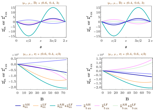
Figure 3: The plots show the variation of the total and axial combination of the transverse $zx$-componets of the magnetoelctric conductivity (in the units of eV) with the angle $\theta$ (upper panel) and the magnitude $B$ in the units of eV² (lower panel). We have used the superscript $\xi$ to indicate that, along the vertical axis, we have plotted the anomalous-Hall-only, Lorentz-force-part-only, and the combined parts, with the colour-coding shown in the plotlegends. While the left subfigures show the behaviour for $\mu_{+}=0.6$ eV and $\mu_{-}=0.4$ eV, the right ones have $\mu_{+}=0.4$ eV and $\mu_{-}=0.6$ eV. The values of the fixed parameters are indicated in each plotlabel. For obtaining all the curves, we have set $v_{0}=0.005$, $\tau=151$ eV^-1, and $T=10$ eV. $\Sigma^{\xi}_{zx}$ and $\Sigma^{\xi}_{5zx}$ are defined in the same way as done for the in-plane components in Eq. (30), indicating the total and the axial parts, respectively, for the two conjugate nodes.

The derivation of the various parts of the magnetoelectric conductivity tensor, as explained in Sec. II.2, has been detailed in Appendix C. Here, we will specifically focus only on the parts involving intranode-only scatterings.

For the intrinsic anomalous Hall part, following the treatment in Appendix C.1, the application of the Sommerfeld expansion yields

$$(\sigma^{\chi,{\text{AH}}}_{\tilde{s}})_{zx} =-\,\frac{e^{3}\,{\tilde{s}}\,v_{0}\,\mathcal{G}_{\tilde{s}}\,B_{y}}{60\,\pi^{2}}\int\frac{d\epsilon}{\epsilon}\left[10\,\epsilon^{2}\,f^{\prime}_{0}(\varepsilon_{\tilde{s}})+e^{2}\,{\tilde{s}}^{2}\,v_{0}^{4}\,\mathcal{G}_{\tilde{s}}^{2}\,B^{2}\,f^{\prime\prime\prime}_{0}(\varepsilon_{\tilde{s}})\right]$$

$$=-\,\frac{e^{3}\,{\tilde{s}}\,v_{0}\,\mathcal{G}_{\tilde{s}}\,B_{y}}{30\,\pi^{2}}\left[5\,\Upsilon_{-1}(\mu_{\chi},T)+6\,B^{2}\,e^{2}\,{\tilde{s}}^{2}\,v_{0}^{4}\,\mathcal{G}_{\tilde{s}}^{2}\,\Upsilon_{-5}(\mu_{\chi},T)\right],$$

$$\Upsilon_{n}(\mu_{\chi},T) =\mu_{\chi}^{n}\left[1+\frac{\pi^{2}\,T^{2}\,n\,(n-1)}{6\,\mu_{\chi}^{2}}+\ldots\right].$$ (21)

The Lorentz-force contribution, derived in Appendix C.3, gives rise to only a nonzero $zx$-component for ${\sigma}^{\chi,\rm LF}_{\tilde{s}}$. Using Eq. eqsigLF, the final expression is captured by

$$\left(\sigma^{\chi,\rm LF}_{\tilde{s}}\right)_{zx} =-\,\frac{e^{3}\,{\tilde{s}}\,\tau^{2}\,v_{0}}{30\,\pi^{2}}\,B_{y}\left[5\,\Upsilon_{1}(\mu_{\chi},T)+e^{2}\,{\tilde{s}}^{4}\,v_{0}^{4}\left(3\,{\tilde{s}}^{2}-8\,\mathcal{G}_{\tilde{s}}\right)B^{2}\,\Upsilon_{-3}(\mu_{\chi},T)\right].$$ (22)

We find a couple of similarities between the intrinsic anomalous Hall part and the Lorentz-force contribution: they both have only odd powers of $B$, and only their out-of-plane Hall components survive. In Fig. 3, we have shown the nature of both these contributions, by choosing some representative parameter values. In a recent experimental investigation [15], the authors have showed the importance of the cubic-in-$B$ terms for multifold semimetals, arising in $\left(\sigma^{\chi,\rm AH}_{s}\right)_{zx}$ and $\left(\sigma^{\chi,\rm LF}_{s}\right)_{zx}$. They have fitted their data using a semiclassical Boltzmann theory, similar to our treatment. Their findings demonstrate that a negative magnetoresistance originates from the chiral anomaly, despite a sizable and detrimental OMM contribution, which was previously unaccounted for. However, a major drawback of their theoretical modelling is that they have simply multiplied the result for a WSM with a factor four in front of the squared brackets, in order to take into account the existence of the two conduction bands of the RSW node.

For the intranode-only in-plane parts, we will consider discuss the inclusion of the pseudomagnetic fields, in addition to the actual magnetic fields. This is because, we are interested in investigating how the strain can affect the linear response. For this purpuse, we subject the sample to elastic deformations [44, 47] such that the net effective magnetic field at a single node is given by

$$\mathbf{B}^{\text{tot}}(\chi)=\mathbf{B}+\chi\,\mathbf{B}_{5}\,,\quad\mathbf{B}_{5}=B_{5}\left(\cos\theta_{5}\,{\mathbf{\hat{x}}}+\sin\theta_{5}\,{\bm{\hat{y}}}\right),$$ (23)

where $\mathbf{B}_{5}$ is the emergent pseudomagnetic field due to strain (cf. Fig. 1). A pseudoelectric field $\mathbf{E}_{5}$, the counterpart of $\mathbf{B}_{5}$, can also be generated on dynamically stretching and compressing the crystal along an axis [71] (for instance, by driving longitudinal sound waves). Then the net effective electric field is $\mathbf{E}^{\text{tot}}(\chi)=\mathbf{E}+\chi\,\mathbf{E}_{5}$. We note that, while the physical electromagnetic fields couple to all the quasiparticles in the same way (irrespective of their chirality), the sign of the coupling of the pseudoelectromagnetic depends on $\chi$, which reflects their axial nature. For this part, we limit ourselves to terms upto $\order{|\mathbf{B}^{\text{tot}}|^{3}}$.

Let us discuss the possibility of the presence of linear-in-$B$ terms in the diagonal components. When the system is subjected purely to homogeneous external fields (without any strain applied on the system), the Onsager-Casimir reciprocity relation [81, 82, 83] for the diagonal components, viz. $(\bar{\sigma}^{\chi}_{\tilde{s}})_{ii}(\mathbf{B})=(\bar{\sigma}^{\chi}_{\tilde{s}})_{ii}(-\mathbf{B})$ , is applicable — it forbids any term in the LMC which has an odd power of $B$, unless the change of sign in $\mathbf{B}$ is compensated for by a change of sign in another parameter in the system [84, 45]. The pseudomagnetic field provides us with such a sign-compensating parameter, leading to

$$(\bar{\sigma}^{\chi}_{\tilde{s}})_{ii}(\mathbf{B},\mathbf{B}_{5})=(\bar{\sigma}^{\chi}_{\tilde{s}})_{ii}(-\mathbf{B},-\mathbf{B}_{5})\,,$$ (24)

thus fulfilling the Onsager-Casimir constraints. This suggests that, in the presence of a nonzero $\mathbf{B}_{5}$, a term linearly dependent on $B$ is possible.

The derivation of the non-anomalous-Hall contribution with intranode-only scatterings (without the Lorentz-force part) has been detailed in Appendices C.2. To analyze the presence of various topological features, we divide up ${\bar{\sigma}}^{\chi}_{s}$ into three parts as follows:

$${\bar{\sigma}}^{\chi}_{\tilde{s}}=\sigma^{\chi,\text{Drude}}_{\tilde{s}}+\sigma^{\chi,\text{BC}}_{\tilde{s}}+\sigma^{\chi,m}_{\tilde{s}}\,.$$ (25)

Here, (1) the first part is the one which is independent of $\mathbf{B}$, also known as the Drude contribution; (2) the second part arises solely due to the effect of the BC and survives when OMM is set to zero; and (3) the third part is the one which goes to zero if OMM is ignored.

III.1 Total and axial in-plane currents without internode scatterings

For the quasiparticles moving in the band $\tilde{s}$, in the vicinity of the node with chirality $\chi$, the in-plane electric current density is

$$\left({\bar{J}}_{\tilde{s}}^{\chi}\right)_{i}=\left({\bar{\sigma}}_{\tilde{s}}^{\chi}\right)_{ij}\,E_{j}^{\text{tot}}(\chi)\,,$$ (26)

where $\left({\bar{\sigma}}_{\tilde{s}}^{\chi}\right)_{ij}$ is given by Eq. (II.2). For a pair of conjugate nodes with chemical potential values $\mu_{+}$ and $\mu_{-}$ [as shown schematically in Fig. 2(a)], we define the total and axial current densities as

$$\mathbf{\bar{J}}(\mu_{+},\mu_{-})=\sum_{\begin{subarray}{c}\chi=\pm 1,\\ \tilde{s}=\frac{1}{2},\frac{3}{2}\end{subarray}}{\mathbf{\bar{J}}}_{\tilde{s}}^{\chi}(\mu_{\chi})\text{ and }\mathbf{\bar{J}}_{5}(\mu_{+},\mu_{-})=\sum_{\begin{subarray}{c}\chi=\pm 1,\\ \tilde{s}=\frac{1}{2},\frac{3}{2}\end{subarray}}\chi\,{\mathbf{\bar{J}}}_{\tilde{s}}^{\chi}(\mu_{\chi})\,,$$ (27)

respectively. The corresponding conductivity tensors are then defined as

$$\bar{\sigma}_{(}\mu_{+},\mu_{-})=\sum_{\chi,\tilde{s}}{\bar{\sigma}}_{\tilde{s}}^{\chi}(\mu_{\chi})\text{ and }\bar{\sigma}_{5}(\mu_{+},\mu_{-})=\sum_{\chi,\tilde{s}}\chi\,{\bar{\sigma}}_{\tilde{s}}^{\chi}(\mu_{\chi})\,.$$ (28)

Using Eq. (28), we find

$$\bar{J}_{i}(\mu_{+},\mu_{-})=\sum_{\tilde{s}}\left[\left(\bar{\sigma}_{\tilde{s}}^{+}(\mu_{+})\right)_{ij}\,E_{+j}+\left(\bar{\sigma}_{\tilde{s}}^{-}(\mu_{-})\right)_{ij}\,E_{-j}\right]=\bar{\sigma}_{ij}(\mu_{+},\mu_{-})\,E_{j}+\bar{\sigma}_{5ij}(\mu_{+},\mu_{-})\,E_{5j}$$

and $$\bar{J}_{5i}(\mu_{+},\mu_{-})=\sum_{\tilde{s}}\left[\left(\bar{\sigma}_{\tilde{s}}^{+}(\mu_{+})\right)_{ij}\,E_{+j}-\left(\bar{\sigma}_{\tilde{s}}^{-}(\mu_{-})\right)_{ij}\,E_{-j}\right]=\bar{\sigma}_{5ij}(\mu_{+},\mu_{-})\,E_{j}+\bar{\sigma}_{ij}(\mu_{+},\mu_{-})\,E_{5j}\,.$$ (29)

Henceforth, we deal with the cases where $\mathbf{E}_{5}=\mathbf{0}$.

From the above expressions for the total and axial currents, we now discuss the behaviour of the total and axial LMC and PHC as functions of $\theta$, which is the angle between $\mathbf{E}$ and $\mathbf{B}$. For plotting the nature of the in-plane components of the conductivity tensor, we define

$$\Sigma_{ij}(\mathbf{B}_{\chi})=\sigma_{ij}(\mu_{+},\mu_{-})-\sigma_{ij}(\mu_{+},\mu_{-})\Big{|}_{\mathbf{B}=\mathbf{B}_{5}=\bm{0}}\text{ and }\Sigma_{5ij}(\mathbf{B}_{\chi})=\sigma_{5ij}(\mu_{+},\mu_{-})-\sigma_{5ij}(\mu_{+},\mu_{-})\Big{|}_{\mathbf{B}=\mathbf{B}_{5}=\bm{0}}$$ (30)

for the total and axial conductivity tensor components, respectively. Here, we have subtracted off the Drude contributions (which refer to the $\mathbf{B}^{\text{tot}}$-independent parts), so that we can focus on the dependence controlled by applied magnetic (and pseudomagnetic) fields. The ranges of the values of the parameters in some realistic scenarios have been shown in Table 1, which we have used in our plots.

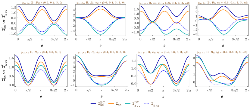
Figure 4: The plots show the variation of the total and axial LMC (in the units of eV) with the angle $\theta$ between $\mathbf{B}$ and $\mathbf{E}$, after subtracting off the Drude part. The superscript “BC” indicates that, for those curves, the OMM contributions have been set to zero. We have used the superscript $\xi$ to indicate that, along the vertical axis, we have plotted the BC-only and OMM-added parts, with the colour-coding shown in the plotlegends. Here, we have included the effects of strain in the form $\mathbf{B}_{5}$. While the upper panel shows the behaviour for $\mu_{+}=0.6$ eV and $\mu_{-}=0.4$ eV, the lower panel has $\mu_{+}=0.4$ eV and $\mu_{-}=0.6$ eV. The values of $B$ and $B_{5}$ (in eV²) are indicated in each plotlabel, along with the value of $\theta_{5}$. For obtaining all the curves, we have set $v_{0}=0.005$, $\tau=151$ eV^-1, and $T=10$ eV.

III.2 Longitudinal magnetoelectric conductivity (LMC)

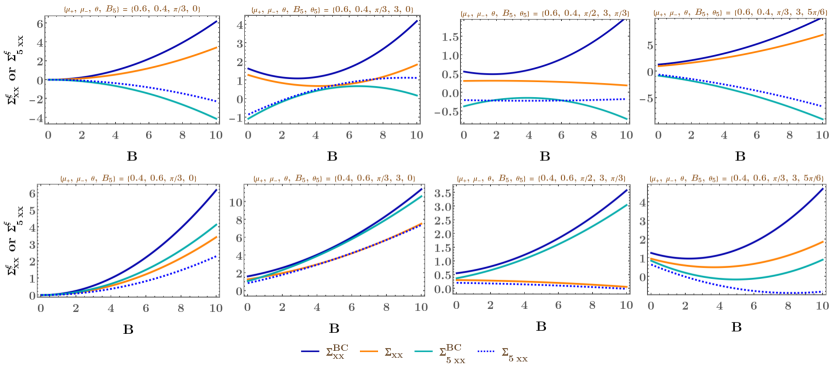
Figure 5: The plots show the variation of the total and axial LMC (in the units of eV) with the magnitude $B$ of the physical magnetic field, after subtracting off the Drude part. The superscript “BC” indicates that, for those curves, the OMM contributions have been set to zero. We have used the superscript $\xi$ to indicate that, along the vertical axis, we have plotted the BC-only and OMM-added parts, with the colour-coding shown in the plotlegends. Here, we have included the effects of strain in the form $\mathbf{B}_{5}$. While the upper panel shows the behaviour for $\mu_{+}=0.6$ eV and $\mu_{-}=0.4$ eV, the lower panel has $\mu_{+}=0.4$ eV and $\mu_{-}=0.6$ eV. The value of $B_{5}$ (in eV²) are indicated in each plotlabel, along with the values of $\theta$ and $\theta_{5}$. For obtaining all the curves, we have set $v_{0}=0.005$, $\tau=151$ eV^-1, and $T=10$ eV.

Using the expressions derived in Appendix C.2, the longitudinal (or diagonal) in-plane component is given by

$$\left({\bar{\sigma}}^{\chi}_{\tilde{s}}\right)_{xx}=\left(\sigma^{\chi,\text{Drude}}_{\tilde{s}}\right)_{xx}+\left(\sigma^{\chi,\text{BC}}_{\tilde{s}}\right)_{xx}+\left(\sigma^{\chi,m}_{\tilde{s}}\right)_{xx}\,,$$ (31)

where

$$\left(\sigma^{\chi,\text{Drude}}_{\tilde{s}}\right)_{xx}=\frac{e^{2}\,\tau}{6\,\pi^{2}\,\tilde{s}\,v_{0}}\,\Upsilon_{2}(\mu_{\chi},T)\,,\quad\left(\sigma^{\chi,\text{BC}}_{\tilde{s}}\right)_{xx}=\frac{e^{4}\,\tau\,{\tilde{s}}^{5}\,v_{0}^{3}}{30\,\pi^{2}}\left[8\,(B^{\text{tot}}_{x})^{2}+(B^{\text{tot}}_{y})^{2}\right]\Upsilon_{-2}(\mu_{\chi},T)\,,$$

$$\left(\sigma^{\chi,m}_{\tilde{s}}\right)_{xx}=\frac{e^{4}\,\tau\,\tilde{s}\,v_{0}^{3}\,\mathcal{G}_{\tilde{s}}}{30\,\pi^{2}}\left[\left(-\,9\,\tilde{s}^{2}+5\,\mathcal{G}_{\tilde{s}}\right)(B^{\text{tot}}_{x})^{2}-3\,\tilde{s}^{2}\,(B^{\text{tot}}_{y})^{2}\right]\Upsilon_{-2}(\mu_{\chi},T)\,.$$ (32)

Adding up the three parts, the total gives us

$$\left({\bar{\sigma}}^{\chi}_{\tilde{s}}\right)_{xx}=\frac{e^{2}\,\tau}{6\,\pi^{2}\,s\,v_{0}}\,\Upsilon_{2}(\mu_{\chi},T)+\frac{e^{4}\,\tau\,{\tilde{s}}\,v_{0}^{3}}{30\,\pi^{2}}\left[{\tilde{s}}^{2}\,(B^{\text{tot}}_{y})^{2}\left({\tilde{s}}^{2}-3\,\mathcal{G}_{s}\right)+(B^{\text{tot}}_{x})^{2}\left(8\,{\tilde{s}}^{4}-9\,{\tilde{s}}^{2}\,\mathcal{G}_{\tilde{s}}+5\,\mathcal{G}_{\tilde{s}}^{2}\right)\right]\Upsilon_{-2}(\mu_{\chi},T)\,.$$ (33)

Let us define the functions

$$f_{x}^{\rm BC}(\tilde{s})=8\,\tilde{s}^{5}\,,\quad f_{x}^{m}(\tilde{s})=\tilde{s}\,\mathcal{G}_{\tilde{s}}\left(-\,9\,\tilde{s}^{2}+5\,\mathcal{G}_{\tilde{s}}\right)\,,\quad f_{y}^{\rm BC}(\tilde{s})=\tilde{s}^{5}\,,\quad f_{y}^{m}(\tilde{s})=-\,3\,{\tilde{s}}^{3}\,\mathcal{G}_{\tilde{s}}\,,$$ (34)

which are the coefficients of the $(B^{\text{tot}}_{x})^{2}$ and $(B^{\text{tot}}_{y})^{2}$ terms, when we consider the BC-only and OMM-effects separately. The supercripts and the subscrtipts indicate which part of the response and which component of $\mathbf{B}^{\text{tot}}$ they are referring to. We find that $f_{x}^{\rm BC}(1/2)=0.25$, $f_{x}^{m}(1/2)=5.6875$, $f_{x}^{\rm BC}(3/2)=60.75$, $f_{x}^{m}(3/2)=-\,18.5625$, $\sum_{\tilde{s}}f_{x}^{\rm BC}(\tilde{s})=61$, $\sum_{\tilde{s}}f_{x}^{m}(\tilde{s})=-\,12.875$, $f_{y}^{\rm BC}(1/2)=0.03125$, $f_{y}^{m}(1/2)=-1.3125$, $f_{y}^{\rm BC}(3/2)=7.59375$, $f_{y}^{m}(3/2)=-\,5.0625$, $\sum_{\tilde{s}}f_{y}^{\rm BC}(\tilde{s})=7.625$, and $\sum_{\tilde{s}}f_{y}^{m}(\tilde{s})=-\,6.375$. These results tell us that

1. $B_{x}^{\text{tot}}$-part: (1) for $\tilde{s}=1/2$, the OMM-part adds up to the BC-only term, thus increasing the overall response; (2) for $\tilde{s}=3/2$, the OMM-part acts in opposition to the BC-only term, thus decreasing the overall response. However, after we sum over the two bands, the contribution from $\tilde{s}=3/2$ dominates, leading to an overall detrimental effect of nonzero OMM, compared to the scenario when we ignore it.

2. $B_{y}^{\text{tot}}$-part: For each of $\tilde{s}=1/2$ and $\tilde{s}=3/2$, the OMM-part acts in opposition to the BC-only term, thus decreasing the overall response. Hence, there is an overall detrimental effect of nonzero OMM compared to the scenario when we ignore it.

We have illustrated the behaviour of $\Sigma_{xx}^{\rm BC}$, $\Sigma_{xx}$, $\Sigma_{5xx}^{\rm BC}$, and $\Sigma_{5xx}$ in Figs. 4 and 5, where the superscript “BC” indicates that the contributions come from the BC-only parts. While the curves in Fig. 4 show the variation of the response as a function of $\theta$, those in Fig. 5 capture the dependence on $B$. In each figure, we have considered cases corresponding to both $\Delta\mu>0$ and $\Delta\mu<0$, where $\Delta\mu\equiv(\mu_{+}-\mu_{-})$. In agreement with our comparison of the $f$-values, we find that a nonzero OMM always reduces the response. In the leftmost subfigure in each panel of Fig. 4, we have the curves with $\mathbf{B}_{5}=\mathbf{0}$. Comparing it with the remaining subfigures in the panel, we find that a nonzero $\mathbf{B}_{5}$-part changes the periodicity with respect to $\theta$ from $\pi$ to $2\pi$, which results from the emergence of terms linearly proportional to $B$, rather than just the $\propto B^{2}$ ones (see Refs. [44, 47] for a similar behaviour in Weyl and multi-Weyl semimetals). Since $\mathbf{B}^{\text{tot}}$ is $\chi$-independent for $\mathbf{B}_{5}=\mathbf{0}$, it is also easy to understand the effect of sign-reversal of $\Delta\mu$ from the leftmost subfigures. As expected, while $\Sigma_{xx}$ is unaffected by the sign of $\Delta\mu$, the curves for $\Sigma_{5xx}$ simply flip with-respect-to the horizontal axis, in tune with the sign-change of $\Delta\mu$. For a nonzero $\mathbf{B}_{5}$, the dependence on $\chi$ (and, consequently, $\mu_{\chi}$) gets complicated, but an overall change in sign is observed.

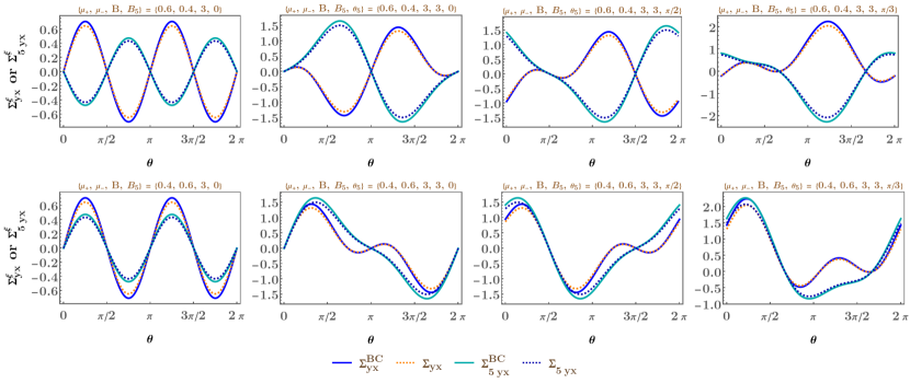
Figure 6: The plots show the variation of the total and axial PHC (in the units of eV) with the angle $\theta$ between $\mathbf{B}$ and $\mathbf{E}$. The superscript “BC” indicates that, for those curves, the OMM contributions have been set to zero. We have used the superscript $\xi$ to indicate that, along the vertical axis, we have plotted the BC-only and OMM-added parts, with the colour-coding shown in the plotlegends. Here, we have included the effects of strain in the form $\mathbf{B}_{5}$. While the upper panel shows the behaviour for $\mu_{+}=0.6$ eV and $\mu_{-}=0.4$ eV, the lower panel has $\mu_{+}=0.4$ eV and $\mu_{-}=0.6$ eV. The values of $B$ and $B_{5}$ (in eV²) are indicated in each plotlabel, along with the value of $\theta_{5}$. For obtaining all the curves, we have set $v_{0}=0.005$, $\tau=151$ eV^-1, and $T=10$ eV.

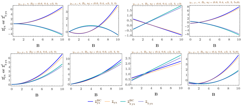
Figure 7: The plots show the variation of the total and axial PHC (in the units of eV) with the magnitude $B$ of the physical magnetic field. The superscript “BC” indicates that, for those curves, the OMM contributions have been set to zero. We have used the superscript $\xi$ to indicate that, along the vertical axis, we have plotted the BC-only and OMM-added parts, with the colour-coding shown in the plotlegends. Here, we have included the effects of strain in the form $\mathbf{B}_{5}$. While the upper panel shows the behaviour for $\mu_{+}=0.6$ eV and $\mu_{-}=0.4$ eV, the lower panel has $\mu_{+}=0.4$ eV and $\mu_{-}=0.6$ eV. The value of $B_{5}$ (in eV²) are indicated in each plotlabel, along with the values of $\theta$ and $\theta_{5}$. For obtaining all the curves, we have set $v_{0}=0.005$, $\tau=151$ eV^-1, and $T=10$ eV.

III.3 Transverse magnetoelectric conductivity (PHC)

Using the expressions derived in Appendix C.2, the transverse in-plane component is given by

$$\left({\bar{\sigma}}^{\chi}_{\tilde{s}}\right)_{yx}=\left(\sigma^{\chi,\text{Drude}}_{\tilde{s}}\right)_{yx}+\left(\sigma^{\chi,\text{BC}}_{\tilde{s}}\right)_{yx}+\left(\sigma^{\chi,m}_{\tilde{s}}\right)_{yx}\,.$$ (35)

where

$$\left(\sigma^{\chi,\text{Drude}}_{\tilde{s}}\right)_{yx}=0\,,\quad\left(\sigma^{\chi,\text{BC}}_{\tilde{s}}\right)_{yx}=\frac{7\,e^{4}\,\tau\,{\tilde{s}}^{5}\,v_{0}^{3}}{30\,\pi^{2}}\,B^{\text{tot}}_{x}\,B^{\text{tot}}_{y}\,\Upsilon_{-2}(\mu_{\chi},T)\,,$$

$$\left(\sigma^{\chi,m}_{\tilde{s}}\right)_{yx}=\frac{e^{4}\,\tau\,{\tilde{s}}\,v_{0}^{3}\,\mathcal{G}_{\tilde{s}}}{30\,\pi^{2}}\,B^{\text{tot}}_{x}\,B^{\text{tot}}_{y}\left(-\,6\,{\tilde{s}}^{2}+5\,\mathcal{G}_{\tilde{s}}\,\right)\Upsilon_{-2}(\mu_{\chi},T)\,.$$ (36)

The addition of the two nonzero parts gives us the planar Hall conductivity (PHC) as

$$\left({\bar{\sigma}}^{\chi}_{\tilde{s}}\right)_{yx}=\frac{e^{4}\,\tau\,{\tilde{s}}\,v_{0}^{3}}{30\,\pi^{2}}\,B^{\text{tot}}_{x}\,B^{\text{tot}}_{y}\left(7\,{\tilde{s}}^{4}-6\,{\tilde{s}}^{2}\,\mathcal{G}_{\tilde{s}}+5\,\mathcal{G}_{\tilde{s}}^{2}\,\right)\Upsilon_{-2}(\mu_{\chi},T)\,.$$ (37)

Let us define the functions

$$g^{\rm BC}(\tilde{s})=7\,\tilde{s}^{5}\,,\quad g^{m}(\tilde{s})=\tilde{s}\,\mathcal{G}_{\tilde{s}}\left(-\,6\,\tilde{s}^{2}+5\,\mathcal{G}_{\tilde{s}}\right)\,,$$ (38)

which are the coefficients of the BC-only and OMM-effects separately. The supercripts indicate which part they are referring to. We find that $g^{\rm BC}(1/2)=0.21875$, $g^{m}(1/2)=6.34375$, $g^{\rm BC}(3/2)=53.1563$, $g^{m}(3/2)=-\,10.9688$, $\sum_{\tilde{s}}g^{\rm BC}(\tilde{s})=53.375$, and $\sum_{\tilde{s}}g^{m}(\tilde{s})=-\,4.625$. These results tell us that (1) for $\tilde{s}=1/2$, the OMM-part adds up to the BC-only term, thus increasing the overall response; (2) for $\tilde{s}=3/2$, the OMM-part acts in opposition to the BC-only term, thus decreasing the overall response. However, after we sum over the two bands, the contribution of the $\tilde{s}=3/2$-band dominates, leading to an overall detrimental effect of nonzero OMM, compared to the scenario when we ignore it.

We have illustrated the behaviour of $\Sigma_{yx}^{\rm BC}$, $\Sigma_{yx}$, $\Sigma_{5yx}^{\rm BC}$, and $\Sigma_{5yx}$ in Figs. 6 and 7, where the superscript “BC” indicates that the contributions come from the BC-only parts. While the curves in Fig. 6 show the variation of the response as a function of $\theta$, those in Fig. 7 capture the dependence on $B$. Analogous to the LMC plots, we have considered cases corresponding to both $\mu_{+}>\mu_{-}$ and $\mu_{+}<\mu_{-}$. In agreement with our comparison of the $g$-values, we find that a nonzero OMM always reduces the response. In the leftmost subfigure in each panel of Fig. 6, we have the curves with $\mathbf{B}_{5}=\mathbf{0}$. Comparing it with the remaining subfigures in the panel, we find that a nonzero $\mathbf{B}_{5}$-part changes the periodicity with respect to $\theta$ from $\pi$ to $2\pi$, which results from the emergence of terms linearly proportional to $B$, rather than just the $\propto B^{2}$ ones (see Refs. [44, 47] for a similar behaviour in Weyl and multi-Weyl semimetals). The relation between the response and the sign of $\Delta\mu$ follows the same trend as discussed for the case of the LMC curves.

IV Magnetothermoelectric conductivity and magnetothermal coefficient

We divide up the expressions for ${\bar{\alpha}}^{\chi}_{s}$ and ${\bar{\ell}}^{\chi}_{s}$, shown in From Eqs. (18) and (20), into three parts as

$${\bar{\alpha}}^{\chi}_{\tilde{s}}=\alpha^{\chi,\text{Drude}}_{\tilde{s}}+\alpha^{\chi,\text{BC}}_{\tilde{s}}+\alpha^{\chi,m}_{\tilde{s}}\text{ and }{\bar{\ell}}^{\chi}_{\tilde{s}}=\ell^{\chi,\text{Drude}}_{\tilde{s}}+\ell^{\chi,\text{BC}}_{\tilde{s}}+\ell^{\chi,m}_{\tilde{s}}\,.$$ (39)

Analogous to the case of ${\bar{\sigma}}^{\chi}_{\tilde{s}}$, (1) the first part stands for the Drude contribution; (2) the second part arises solely due to the effect of the BC and survives when OMM is set to zero; and (3) the third part is the one which goes to zero if OMM is ignored.

IV.1 Magnetothermoelectric conductivity

The longitudinal (or diagonal) in-plane component of ${\bar{\alpha}}^{\chi}_{\tilde{s}}$, also known as the longitudinal thermoelectric coefficient (LTEC), is given by

$$\left({\bar{\alpha}}^{\chi}_{\tilde{s}}\right)_{xx}=\left(\alpha^{\chi,\text{Drude}}_{\tilde{s}}\right)_{xx}+\left(\alpha^{\chi,\text{BC}}_{\tilde{s}}\right)_{xx}+\left(\alpha^{\chi,m}_{\tilde{s}}\right)_{xx}\,,$$ (40)

where

$$\left(\alpha^{\chi,\text{Drude}}_{\tilde{s}}\right)_{xx}=-\,\frac{e\,\tau\,\mu_{\chi}\,T}{9\,{\tilde{s}}\,v_{0}}\,,\quad\left(\alpha^{\chi,\text{BC}}_{\tilde{s}}\right)_{xx}=\frac{e^{3}\,\tau\,{\tilde{s}}^{5}\,v_{0}^{3}\,T}{45\,\mu_{\chi}^{3}}\left[8\,(B^{\text{tot}}_{x})^{2}+(B^{\text{tot}}_{y})^{2}\right],$$

$$\left(\alpha^{\chi,m}_{\tilde{s}}\right)_{xx}=\frac{e^{3}\,\tau\,{\tilde{s}}\,v_{0}^{3}\,\mathcal{G}_{\tilde{s}}\,T}{45\,\mu_{\chi}^{3}}\left[(B^{\text{tot}}_{x})^{2}\left(-9\,{\tilde{s}}^{2}+5\,\mathcal{G}_{\tilde{s}}\right)-3\,{\tilde{s}}^{2}\,(B^{\text{tot}}_{y})^{2}\right].$$ (41)

The total expression of the LTEC reads

$$\left({\bar{\alpha}}^{\chi}_{\tilde{s}}\right)_{xx} =-\,\frac{e\,\tau\,\mu_{\chi}\,T}{9\,{\tilde{s}}\,v_{0}}+\frac{e^{3}\,\tau\,{\tilde{s}}\,v_{0}^{3}\,T}{45\,\mu_{\chi}^{3}}\left[(B^{\text{tot}}_{x})^{2}\left(8\,{\tilde{s}}^{4}-9\,{\tilde{s}}^{2}\,\mathcal{G}_{\tilde{s}}+5\,\mathcal{G}_{\tilde{s}}^{2}\right)+{\tilde{s}}^{2}\,(B^{\text{tot}}_{y})^{2}\left({\tilde{s}}^{2}-3\,\mathcal{G}_{\tilde{s}}\right)\right].$$ (42)

The transverse in-plane component of ${\bar{\alpha}}^{\chi}_{\tilde{s}}$, also known as the transverse thermoelectric coefficient (TTEC), is given by

$$\left({\bar{\alpha}}^{\chi}_{\tilde{s}}\right)_{yx}=\left(\alpha^{\chi,\text{Drude}}_{\tilde{s}}\right)_{yx}+\left(\alpha^{\chi,\text{BC}}_{\tilde{s}}\right)_{yx}+\left(\alpha^{\chi,m}_{\tilde{s}}\right)_{yx}\,,$$ (43)

where

$$\left(\alpha^{\chi,\text{Drude}}_{\tilde{s}}\right)_{yx}=0\,,\quad\left(\alpha^{\chi,\text{BC}}_{\tilde{s}}\right)_{yx}=\frac{7\,e^{3}\,\tau\,{\tilde{s}}^{5}\,v_{0}^{3}\,T}{45\,\mu_{\chi}^{3}}\,B^{\text{tot}}_{x}\,B^{\text{tot}}_{y}\,,\quad\left(\alpha^{\chi,m}_{\tilde{s}}\right)_{yx}=\frac{e^{3}\,\tau\,\tilde{s}\,v_{0}^{3}\,T}{45\,\mu_{\chi}^{3}}\,B^{\text{tot}}_{x}\,B^{\text{tot}}_{y}\left(-6\,{\tilde{s}}^{2}\,\mathcal{G}_{\tilde{s}}+5\,\mathcal{G}_{\tilde{s}}^{2}\right).$$ (44)

The total expression of the TTEC reads

$$\left({\bar{\alpha}}^{\chi}_{\tilde{s}}\right)_{xx}=\frac{e^{3}\,\tau\,{\tilde{s}}\,v_{0}^{3}\,T}{45\,\mu_{\chi}^{3}}\,B^{\text{tot}}_{x}\,B^{\text{tot}}_{y}\left(7\,{\tilde{s}}^{4}-6\,{\tilde{s}}^{2}\,\mathcal{G}_{\tilde{s}}+5\,\mathcal{G}_{\tilde{s}}^{2}\right).$$ (45)

IV.2 Magnetothermal coefficient

The longitudinal (or diagonal) in-plane component of ${\bar{\ell}}^{\chi}_{\tilde{s}}$ is given by

$$\left({\bar{\ell}}^{\chi}_{\tilde{s}}\right)_{xx}=\left(\ell^{\chi,\text{Drude}}_{\tilde{s}}\right)_{xx}+\left(\ell^{\chi,\text{BC}}_{\tilde{s}}\right)_{xx}+\left(\ell^{\chi,m}_{\tilde{s}}\right)_{xx}\,,$$ (46)

where

$$\left(\ell^{\chi,\text{Drude}}_{\tilde{s}}\right)_{xx}=0\,,\quad\left(\ell^{\chi,\text{BC}}_{\tilde{s}}\right)_{xx}=\frac{e^{2}\,s^{5}\,\tau\,v_{0}^{3}}{90\,\pi^{2}\,\mu_{\chi}^{2}\,T}\left(\pi^{2}T^{2}-6\,\mu_{\chi}^{2}\right)\left[8\,(B^{\text{tot}}_{x})^{2}+(B^{\text{tot}}_{y})^{2}\right]\,,$$

$$(\ell^{\chi,m}_{\tilde{s}})_{xx}=\frac{e^{2}\,{\tilde{s}}\,\tau\,v_{0}^{3}\,\mathcal{G}_{\tilde{s}}}{90\,\pi^{2}\,\mu_{\chi}^{2}\,T}\left[3\,{\tilde{s}}^{2}\left\{(B^{\text{tot}}_{x})^{2}\left(32\,\mu_{\chi}^{2}-3\,\pi^{2}\,T^{2}\right)+(B^{\text{tot}}_{y})^{2}\left(\pi^{2}\,T^{2}-4\,\mu_{\chi}^{2}\right)\right\}+5\,\mathcal{G}_{\tilde{s}}\left\{(B^{\text{tot}}_{x})^{2}\left(\pi^{2}\,T^{2}-9\,\mu_{\chi}^{2}\right)+3\,\mu_{\chi}^{2}\,(B^{\text{tot}}_{y})^{2}\right\}\right].$$ (47)

The sum of all the parts reads

$$\left({\bar{\ell}}^{\chi}_{\tilde{s}}\right)_{xx} =\frac{e^{2}\,{\tilde{s}}\,\tau\,v_{0}^{3}}{90\,\pi^{2}\,\mu_{\chi}^{2}\,T}\bigg{[}-3\,{\tilde{s}}^{2}\,\mathcal{G}_{\tilde{s}}\left\{(B^{\text{tot}}_{x})^{2}\left(3\,\pi^{2}\,T^{2}-32\,\mu_{\chi}^{2}\right)+(B^{\text{tot}}_{y})^{2}\left(\pi^{2}\,T^{2}-4\,\mu_{\chi}^{2}\right)\right\}$$

$$\hskip 65.44142pt+5\,\mathcal{G}_{\tilde{s}}^{2}\left\{(B^{\text{tot}}_{x})^{2}\left(\pi^{2}\,T^{2}-9\,\mu_{\chi}^{2}\right)+3\,\mu_{\chi}^{2}\,(B^{\text{tot}}_{y})^{2}\right\}+{\tilde{s}}^{4}\left(\pi^{2}\,T^{2}-6\,\mu_{\chi}^{2}\right)\left\{8\,(B^{\text{tot}}_{x})^{2}+(B^{\text{tot}}_{y})^{2}\right\}\bigg{]}\,.$$ (48)

The transverse in-plane component of ${\bar{\ell}}^{\chi}_{\tilde{s}}$ is given by

$$\left({\bar{\ell}}^{\chi}_{\tilde{s}}\right)_{yx}=\left(\ell^{\chi,\text{Drude}}_{\tilde{s}}\right)_{yx}+\left(\ell^{\chi,\text{BC}}_{\tilde{s}}\right)_{yx}+\left(\ell^{\chi,m}_{\tilde{s}}\right)_{yx}\,,$$ (49)

where

$$\left(\ell^{\chi,\text{Drude}}_{\tilde{s}}\right)_{yx}=0\,,\quad\left(\ell^{\chi,\text{BC}}_{\tilde{s}}\right)_{yx}=\frac{7\,e^{2}\,{\tilde{s}}^{5}\,\tau\,v_{0}^{3}\,B^{\text{tot}}_{x}\,B^{\text{tot}}_{y}\left(\pi^{2}\,T^{2}-6\,\mu_{\chi}^{2}\right)}{90\,\pi^{2}\,\mu_{\chi}^{2}\,T}\,,$$

$$\left(\ell^{\chi,m}_{\tilde{s}}\right)_{yx}=\frac{e^{2}\,{\tilde{s}}\,\tau\,v_{0}^{3}\,\mathcal{G}_{\tilde{s}}\,B^{\text{tot}}_{x}\,B^{\text{tot}}_{y}\left[-\,6\,{\tilde{s}}^{2}\left(\pi^{2}\,T^{2}-14\,\mu_{\chi}^{2}\right)+5\,\mathcal{G}_{\tilde{s}}\left(\pi^{2}\,T^{2}-12\,\mu_{\chi}^{2}\right)\right]}{90\,\pi^{2}\,\mu_{\chi}^{2}\,T}\,.$$ (50)

The sum of all the parts reads

$$\left({\bar{\ell}}^{\chi}_{\tilde{s}}\right)_{yx}=\frac{e^{2}\,{\tilde{s}}\,\tau\,v_{0}^{3}\,B^{\text{tot}}_{x}\,B^{\text{tot}}_{y}\left[-\,6\,{\tilde{s}}^{2}\,\mathcal{G}_{\tilde{s}}\left(\pi^{2}\,T^{2}-14\,\mu_{\chi}^{2}\right)+5\,\mathcal{G}_{\tilde{s}}^{2}\left(\pi^{2}\,T^{2}-12\,\mu_{\chi}^{2}\right)+7\,{\tilde{s}}^{4}\left(\pi^{2}\,T^{2}-6\,\mu_{\chi}^{2}\right)\right]}{90\,\pi^{2}\,\mu_{\chi}^{2}\,T}\,.$$ (51)

IV.3 Mott relation and Wiedemann-Franz law

From the explicit expressions of $\bar{\sigma}^{\chi}_{\tilde{s}}$ and $\bar{\alpha}^{\chi}_{\tilde{s}}$ that we have demonstrated, we can immediately spot the relation

$$\partial_{\mu_{\chi}}(\bar{\sigma}^{\chi}_{\tilde{s}})_{ij}=-\frac{3\,e}{\pi^{2}\,T}\left(\bar{\alpha}^{\chi}_{\tilde{s}}\right)_{ij}+\order{T^{2}}$$ (52)

being satisfied. This is equivalent to satisfying the Mott relation, which holds in the limit $T\rightarrow 0$ [85]. In particular, we find that the Mott relation continues to hold in the presence of OMM, agreeing with the results of Ref. [86], where generic settings for the linear response have been considered. From the explicit expressions of $\sigma^{\chi}_{\tilde{s}}$ and $\ell^{\chi}_{\tilde{s}}$, we find another relation relation, namely,

$$(\bar{\sigma}^{\chi}_{\tilde{s}})_{ij}=\frac{3\,e^{2}}{\pi^{2}\,T}\left(\bar{\ell}^{\chi}_{\tilde{s}}\right)_{ij}+\order{T^{2}}$$ (53)

being satisfied. This is equivalent to satisfying the Wiedemann-Franz law, which again holds in the limit $T\rightarrow 0$ [85]. Therefore, we find that the Wiedemann-Franz law also continues to be valid in the presence of OMM. Due to the Mott relation and the Wiedemann-Franz law, the behaviour of $(\bar{\alpha}^{\chi}_{\tilde{s}})_{ij}$ and $\left(\bar{\ell}^{\chi}_{\tilde{s}}\right)_{ij}$ can be readily inferred from that of $(\bar{\sigma}^{\chi}_{\tilde{s}})_{ij}$. Hence, we do not provide separate plots and discussions for the $\bar{\alpha}^{\chi}_{\tilde{s}}$ and $\bar{\ell}^{\chi}_{\tilde{s}}$ tensors.

V Inclusion of internode scatterings

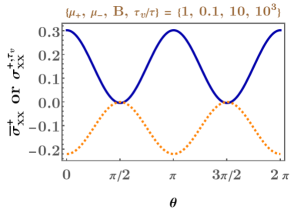
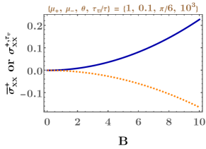
Figure 8: The variation of the intranode-only (dark blue) and internode-only (dotted orange) contributions to the LMC (in the units of eV) with (a) the angle $\theta$ between $\mathbf{B}$ and $\mathbf{E}$; (b) $B$, after subtracting off the Drude part. Here, we have considered a single node of chirality $+1$. The values of the fixed parameters are indicated in the plotlabels. For obtaining all the curves, we have set $v_{0}=0.005$, $\tau=151$ eV^-1, and $T=10$ eV.

Till now, we have focussed only on intranode scattering, ignoring any internode processes. This section will be dedicated to understanding how the internode scatterings affect the magnetoconductivity tensor. We will not discuss the corresponding influence on the magnetothermoelectric and magnetothermal coefficients because, as we have seen, the Mott relation and the Wiedemann-Franz law ensure that their nature can be derived from that of the magnetoconductivity tensor.

Since the survival of the internode part solely depends on the presence of a nonzero $\mathbf{B}\cdot\mathbf{E}$, there is no Drude part. Using the derivations of Appendix C.4, we find that

$$(\sigma^{\chi,\tau_{v}}_{\tilde{s}})_{xx}=-\,\frac{\chi\,e^{4}\,v_{0}^{3}\left(\tau_{v}-\tau\right)}{72\,\pi^{2}\,\mu_{\text{eq}}^{2}\,{\tilde{s}}^{2}}\,B_{x}^{2}\left(9\,{\tilde{s}}^{4}-9\,{\tilde{s}}^{2}\,\mathcal{G}_{\tilde{s}}+2\,\mathcal{G}_{\tilde{s}}^{2}\right),$$

$$(\sigma^{\chi,\tau_{v}}_{\tilde{s}})_{yx}=-\,\frac{\chi\,e^{4}\,v_{0}^{3}\left(\tau_{v}-\tau\right)}{72\,\pi^{2}\,\mu_{\text{eq}}^{2}\,{\tilde{s}}^{2}}\,B_{x}\,B_{y}\left(9\,{\tilde{s}}^{4}-9\,{\tilde{s}}^{2}\,\mathcal{G}_{\tilde{s}}+2\,\mathcal{G}_{\tilde{s}}^{2}\right),$$ (54)

where $\mu_{\text{eq}}=\left(\mu_{+}+\mu_{-}\right)/2$, and the results are now dependent on the internode-process relaxation time, $\tau_{v}$. Clearly, for $\mu_{+}=\mu_{-}$, we have $(\sigma^{+,\tau_{v}}_{\tilde{s}})_{ij}=-(\sigma^{-,\tau_{v}}_{\tilde{s}})_{ij}$, due to the overall proportionality to a $\chi$-factor. This is because the internode processes are inherently connected to an imbalance of the values of the local chemical potential at the pair of conjugate nodes, and the relaxation tries to bring about a global equilibrium value. When the global equilibrium is reached, no net current flows from one node to the other.

In Figs. 8 and 9, we have illustrated the behaviour of the internode part of the LMC and the PHC, respectively. We have considered the contribution from a single node of positive chirality, and have compared the internode-only-scattering part with the intreanode-only-scattering part. We need to take a high value of $\tau_{v}/\tau$ satisfying the physical condition of $\tau_{v}\gg\tau$. This is because, under these conditions, the system first reaches local equilibrium through intraband scattering and, thereafter, achieves global equilibrium through interband scattering [87].

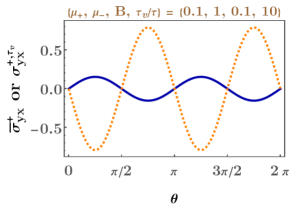
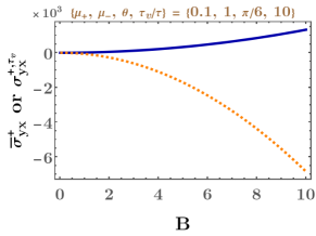
Figure 9: The variation of the intranode-only (dark blue) and internode-only (dotted orange) contributions to the PHC (in the units of eV) with (a) the angle $\theta$ between $\mathbf{B}$ and $\mathbf{E}$; (b) $B$. Here, we have considered a single node of chirality $+1$. The values of the fixed parameters are indicated in the plotlabels. For obtaining all the curves, we have set $v_{0}=0.005$, $\tau=151$ eV^-1, and $T=10$ eV.

VI Summary and future perspectives

In this paper, we have considered planar Hall and planar thermal Hall setups, where an RSW semimetal is subjected to the combined effects of an electric field $\mathbf{E}$ and/or temperature gradient $\nabla_{\mathbf{r}}T$. The $\mathbf{E}$ and $\nabla_{\mathbf{r}}T$ fields are assumed to be along the same direction. Since we have considered an isotropic RSW material, without any rotational-symmetry-breaking term (e.g., the tilting of the nodes), the plane in which the fields are applied makes no difference. For computing the in-plane components of the response tensors, we have added an elastic deformation which gives rise to a chirality-dependent effective magnetic field $\mathbf{B}^{\text{tot}}$ consisting of two parts — (1) the physical magnetic field $\mathbf{B}$ and (2) an emergent axial magnetic field $\mathbf{B}_{5}$. This is captured by defining $\mathbf{B}^{\text{tot}}=\mathbf{B}+\chi\,\mathbf{B}_{5}$ for the corresponding nodal point. Due to the chiral nature of $\mathbf{B}_{5}$, its presence makes it possible to have linear-in-$B$ terms in the linear-response coefficients, which otherwise is ruled out in accordance of the Onsager-Casimir reciprocity relations. In all our calculations, the effects of the nontrivial topology of the RSW bandstructure have been captured through the inclusion of both the BC and the OMM. In many earlier works, the response in such nodal-point semimetals have been computed neglecting the OMM parts. However, following the treatment of some recent papers [42, 88, 43, 47], here we have included the OMM terms in a systematic way, and have emphasized on the importance of the consequence of a nonzero OMM, which anyway arises at the same footing as the BC.

The RSW semimetals provide a richer structure for obtaining the linear-response coefficients, compared to the WSMs, because of the fact that the former consists of four bands (rather than just two). Although each band still shows a linear-in-momentum dispersion, just like a WSM node, the constant of proportionality with $k$ changes from band to band. Furthermore, needless to say, the bands have differing BC and OMM, which then provide unequal contributions to the net response. We have clearly pointed out these aspects in our explicit derivations of the electric conductivity, thermoelectric conductivity, and thermal coefficient tensors, in the presence of a non-quantizing magnetic field. In particular, we have found that the OMM-contributed terms may oppose or add up to the BC-only parts, depending on which band we are considering.

First, we have computed the response by only considering collisions arising from intranode processes, assuming a momentum-independent relaxation time $\tau$. After analyzing their characteristics, we have proceeded to include new terms which arise on having internode scatterings of nonzero amplitudes, characterized by another relaxation time $\tau_{v}$. Through this procedure, we have been able to compare the roles of the two kinds of terms.

Last, but not the least, we have determined the out-of-plane response comprising the intrinsic anomalous Hall and the Lorentz-force-contributed currents. These terms inherently consist of only odd powers of $B$, giving rise to linear-in-$B$ and linear-in-$B^{3}$ dependence when we limit ourselves to expanding the expressions upto order $B^{3}$. These terms corroborate the findings of some recent experimental results [15], which have found clear signature of the importance of the $\order{B^{3}}$ terms in multifold semimetals. We have also pointed out some limitations of the theoretical modelling they have used to fit their data.

In our calculations, we have assumed the same relaxation times to be applicable for all the bands. In the future, we would like to improve our calculations by going beyond the relaxation-time approximation, which involves actually computing the collision integrals for all relevant scattering processes [42], rather than just using phenomenological values of momentum-independent relaxation times.

Other directions worthwhile to be pursued are repeating our calculations for tilted RSW nodes [42, 88, 45], as tilting is expected in generic materials. Furthermore, although we have considered the limit of weak non-quantizing magnetic field in this paper, we would like to study the influence of a strong quantizing magnetic field. This would involve incorporating the formation of the discrete Landau levels [89, 38, 54, 55]. Lastly, if we want to move into the realm of linear and nonlinear response in the presence of strong disorder and/or strong interactions, we need to consider many-body techniques applicable for strongly-correlated systems [90, 62, 91, 92, 93, 94, 95, 96].

Appendix A Linear response from semiclassical Boltzmann equations

In this appendix, we review the semiclassical Boltzmann formalism [85, 46, 44], which is the used to determine the transport coefficients in the regime of linear response. There exists an externally applied magnetic field $\mathbf{B}$, which we assume to be small in magnitude, leading to a small cyclotron frequency $\omega_{c}=e\,B/(m^{*}\,c)$ [where $m^{*}$ is the effective mass with the magnitude $\sim 0.11\,m_{e}$ [97], with $m_{e}$ denoting the electron mass]. This allows us to ignore quantized Landau levels, with the regime of validity of our approximations given by $\hbar\,\omega_{c}\ll\mu$, where $\mu$ is the Fermi level [i.e., the energy at which the chemical potential cuts the energy band(s)]. Furthermore, we will derive the expressions following from a relaxation-time approximation for the collision integral, which involves using a momentum-independent relaxation time, which implies that we treated it as a phenomenological parameter.

To start with, we assume that only internode scatterings matter in the collision integral, such that we consider only the corresponding relaxation time $\tau$. In particular, we focus on the transport for a single node of chirality $\chi$. The derivation here closely follows the arguments outlined in Refs. [46, 44, 47]

For a 3d system, we define the Fermi-Dirac distribution function $f_{s}^{\chi}(\mathbf{r},\mathbf{k},t)$ for the quasiparticles occupying a Bloch band labelled by the index $s$, with the crystal momentum $\mathbf{k}$ and dispersion $\varepsilon_{s}(\mathbf{k})$, such that

$$dN_{s}=g_{s}\,f_{s}(\mathbf{r},\mathbf{k},t)\,\frac{d^{3}\mathbf{k}}{(2\,\pi)^{3}}\,d^{3}\mathbf{r}$$ (55)

is the number of particles occupying an infinitesimal phase space volume of $dV_{p}=\frac{d^{3}\mathbf{k}}{(2\,\pi)^{3}}\,d^{3}\mathbf{r}$, centered at $\left\{\mathbf{r},\mathbf{k}\right\}$ at time $t$. Here, $g_{s}$ denotes the degeneracy of the band. In the presence of a nontrivial topology in the bandstructure, a nonzero orbital magnetic moment (OMM) is induced, and there appears a Zeeman-like correction to the energy due to the OMM, which we denote by $\eta_{s}^{\chi}(\mathbf{k})$. Hence, we define the OMM-corrected dispersion and the corresponding modified Bloch velocity as

$$\xi^{\chi}_{s}({\mathbf{k}})=\varepsilon_{s}(\mathbf{k})\,+\,\eta^{\chi}_{s}(\mathbf{k}),\quad\text{and }\quad\bm{w}^{\chi}_{s}(\mathbf{k})=\nabla_{\mathbf{k}}\varepsilon_{s}(\mathbf{k})+\nabla_{\mathbf{k}}\eta^{\chi}_{s}(\mathbf{k})\,,$$ (56)

respectively. The Hamilton’s equations of motion for the quasiparticles, under the influence of static electric ($\mathbf{E}$) and magnetic ($\mathbf{B}$) fields, are given by [85, 49, 98]

$$\dot{\mathbf{r}} =\nabla_{\mathbf{k}}\,\xi^{\chi}_{s}+\dot{\mathbf{k}}\,\crossproduct\,\mathbf{\Omega}^{\chi}_{s}\text{ and }\dot{\mathbf{k}}=e\left({\mathbf{E}}\,+\,\dot{\mathbf{r}}\,\crossproduct\,{\mathbf{B}}\right)$$

$$\Rightarrow \,\dot{\mathbf{r}}=\mathcal{D}^{\chi}_{s}\left[\bm{w}^{\chi}_{s}+e\,({\mathbf{E}}\crossproduct\mathbf{\Omega}^{\chi}_{s})\,+e\,(\mathbf{\Omega}^{\chi}_{s}\cdot\bm{w}^{\chi}_{s})\,\mathbf{B}\right]\text{ and }\dot{\mathbf{k}}=e\,\mathcal{D}^{\chi}_{s}\,\left[{\mathbf{E}}+\left(\bm{w}^{\chi}_{s}\crossproduct{\mathbf{B}}\right)+e\left({\mathbf{E}}\cdot{\mathbf{B}}\right)\mathbf{\Omega}^{\chi}_{s}\right].$$ (57)

where $-\,e$ is the charge carried by each quasiparticle. Furthermore,

$$\mathcal{D}^{\chi}_{s}=\frac{1}{1+\,e\left(\mathbf{B}\cdot\mathbf{\Omega}^{\chi}_{s}\right)}$$ (58)

is the factor which modifies the phase volume element from $dV_{p}$ to $(\mathcal{D}^{\chi}_{s})^{-1}\,dV_{p}$, such that the Liouville’s theorem (in the absence of collisions) continues to hold in the presence of a nonzero BC [99, 100, 101, 102].

Incorporating all these ingredients, the kinetic equation of the quasiparticles is finally given by [103, 34]

$$\mathcal{D}^{\chi}_{s}\,\left[\partial_{t}+\left\{\bm{w}^{\chi}_{s}+e\,{\mathbf{E}}\crossproduct\mathbf{\Omega}^{\chi}_{s}+e\left({\mathbf{\Omega}}^{\chi}_{s}\cdot\bm{w}^{\chi}_{s}\right)\mathbf{B}\right\}\cdot\nabla_{\mathbf{r}}-e\left({\mathbf{E}}+\bm{w}^{\chi}_{s}\crossproduct{\mathbf{B}}\right)\cdot\nabla_{\mathbf{k}}-e^{2}\left({\mathbf{E}}\cdot{\mathbf{B}}\right)\Omega^{\chi}_{s}\cdot\nabla_{\mathbf{k}}\right]f_{s}^{\chi}=I_{\rm coll}\,.$$ (59)

which results from the Liouville’s equation in the presence of scattering events. On the right-hand side, $I_{\rm coll}$ denotes the collision integral, which corrects the Liouville’s equation, taking into account the collisions of the quasiparticles.

Let the contributions to the average DC electric and thermal current densities from the quasiparticles, associated with the band $s$ at the node with chirality $\chi$, be ${\mathbf{J}}_{s}^{\chi}$ and ${\mathbf{J}}^{{\rm th},\chi}_{s}$, respectively. The linear-response matrix, which relates the resulting generalized current densities to the driving electric potential gradient and temperature gradient, is expressed as

$$\begin{bmatrix}\left(J_{s}^{\chi}\right)_{i}\vspace{0.2 cm}\\ \left({J}_{s}^{{\rm th},\chi}\right)_{i}\end{bmatrix} =\sum\limits_{j}\begin{bmatrix}\left(\sigma_{s}^{\chi}\right)_{ij}&\left(\alpha_{s}^{\chi}\right)_{ij}\vspace{0.2 cm}\\ T\left(\alpha_{s}^{\chi}\right)_{ij}&\left(\ell_{s}^{\chi}\right)_{ij}\end{bmatrix}\begin{bmatrix}E_{j}\vspace{0.2 cm}\\ -\,{\partial_{j}T}\end{bmatrix},$$ (60)

where $\{i,j\}\in\{x,\,y,\,z\}$ indicates the Cartesian components of the current density vectors and the response tensors in 3d. Using the explicit forms of [32, 34] and the thermal current density [104, 103] are captured by the following:

$${\mathbf{J}}^{\chi}_{s} =-\,e\,g_{s}\int\frac{d^{3}\mathbf{k}}{(2\,\pi)^{3}}\,(\mathcal{D}^{\chi}_{s})^{-1}\,\dot{\mathbf{r}}\,f_{s}^{\chi}(\mathbf{r},\mathbf{k})\text{ and }\mathbf{J}^{\rm th,\chi}_{s}=g_{s}\int\frac{d^{3}\mathbf{k}}{(2\,\pi)^{3}}\,(\mathcal{D}^{\chi}_{s})^{-1}\,\dot{\mathbf{r}}\,\left(\xi^{\chi}_{s}-\mu_{\chi}\right)f_{s}^{\chi}(\mathbf{r},\mathbf{k})$$

$$\Rightarrow{\mathbf{J}}^{\chi}_{s} =-\,e\,g_{s}\int\frac{d^{3}\mathbf{k}}{(2\,\pi)^{3}}\,\left[\bm{w}^{\chi}_{s}+e\,({\mathbf{E}}\crossproduct\mathbf{\Omega}^{\chi}_{s})+e\,(\mathbf{\Omega}^{\chi}_{s}\cdot\bm{w}^{\chi}_{s})\,\mathbf{B}\right]\,f_{s}^{\chi}(\mathbf{r},\mathbf{k})$$

and $$\mathbf{J}^{\rm th,\chi}_{s}=g_{s}\int\frac{d^{3}\mathbf{k}}{(2\,\pi)^{3}}\left[\bm{w}^{\chi}_{s}+e\,({\mathbf{E}}\crossproduct\mathbf{\Omega}^{\chi}_{s})\,+e\,(\mathbf{\Omega}^{\chi}_{s}\cdot\bm{w}^{\chi}_{s})\,\mathbf{B}\right]\left(\xi^{\chi}_{s}-\mu_{\chi}\right)f_{s}^{\chi}(\mathbf{r},\mathbf{k})\text{ [using Eq.~{}\eqref{eqrkdot}].}$$ (61)

Comparing with Eq. (60), we extract the final expressions for the linear-response coefficients. The notations $\sigma^{\chi}_{s}$ and $\alpha^{\chi}_{s}$ represents the magnetoelectric conductivity and the magnetothermoelectric conductivity tensors, respectively. The latter determines the Peltier ($\Pi^{\chi}_{s}$), Seebeck ($S^{\chi}_{s}$), and Nernst coefficients. The third tensor $\ell^{\chi}$ represents the linear response relating the thermal current density to the temperature gradient, at a vanishing electric field. $S^{\chi}$ , $\Pi^{\chi}$, and the magnetothermal coefficient tensor $\kappa^{\chi}$ (which provides the coefficients between the heat current density and the temperature gradient at vanishing electric current) are related as [85, 46]:

$$\left(S_{s}^{\chi}\right)_{ij}=\sum\limits_{i^{\prime}}\left(\sigma^{\chi}_{s}\right)^{-1}_{ii^{\prime}}\left(\alpha^{\chi}_{s}\right)_{i^{\prime}j}\,,\quad\left(\Pi_{s}^{\chi}\right)_{ij}=T\sum\limits_{i^{\prime}}\left(\alpha^{\chi}_{s}\right){ii^{\prime}}\left(\sigma^{\chi}_{s}\right)^{-1}_{i^{\prime}j}\,,\quad\left(\kappa_{s}^{\chi}\right)_{ij}=\left(\ell^{\chi}_{s}\right)_{ij}-T\sum\limits_{i^{\prime},\,j^{\prime}}\left(\alpha^{\chi}_{s}\right)_{ii^{\prime}}\left(\sigma_{s}^{\chi}\right)^{-1}_{i^{\prime}j^{\prime}}\left(\alpha^{\chi}_{s}\right)_{j^{\prime}j}\,.$$ (62)

Since $\ell_{s}^{\chi}$ determines the first term in the magnetothermal coefficient tensor $\kappa_{s}^{\chi}$, here we will loosely refer to $\ell^{\chi}$ itself as the magnetothermal coefficient.

A.1 Ignoring internode scattering

To start with, we use the relaxation-time approximation, with only intranode and intraband scattering processes taken into account. The neglect of interband scatterings is justified if only pseudospin-conserving processes are allowed. Under these approximations/assumptions, the collision integral takes the form of

$$I_{\rm coll}=\frac{f^{(0)}_{s,\chi}(\mathbf{r},\mathbf{k})-f_{s}^{\chi}(\mathbf{r},\mathbf{k},t)}{\tau}\,,$$ (63)

where the time-independent distribution function

$$f^{(0)}_{s,\chi}(\mathbf{r},\mathbf{k})\equiv f_{0}\big{(}\xi^{\chi}_{s}(\mathbf{k}),\mu_{\chi},T(\mathbf{r})\big{)}=\frac{1}{1+\exp[\frac{\xi^{\chi}_{s}(\mathbf{k})-\mu_{\chi}}{T(\mathbf{r})}]}\,,$$ (64)

describes a local equilibrium situation at the subsystem centred at position $\mathbf{r}$, at the local temperature $T(\mathbf{r})$, and with a spatially uniform chemical potential $\mu_{\chi}$.

In order to obtain a solution to the full Boltzmann equation for small time-independent values of $\mathbf{E}$ and $\nabla_{\mathbf{r}}T$, we assume a small deviation, $\delta f_{s}^{\chi}(\mathbf{r},\mathbf{k})$, from the equilibrium distribution of the quasiparticles. We have not included any explicit time-dependence in it since the applied fields and gradients are static. Hence, the nonequilibrium time-independent distribution function can be expressed as

$$f_{s}^{\chi}(\mathbf{r},\mathbf{k},t)\equiv f_{s}^{\chi}(\mathbf{r},\mathbf{k})=f_{0}+\delta f_{s}^{\chi}(\mathbf{r},\mathbf{k})\,,$$ (65)

where we have suppressed showing explicitly the dependence of $f_{0}$ on $\xi^{\chi}_{s}(\mathbf{k})$, $\mu_{\chi}$, and $T(\mathbf{r})$. At this point, the magnetic field is not assumed to be small, except for the fact that it should not be so large that the energy levels of the systems get modified by the formation of discrete Landau levels.

The gradients of the equilibrium distribution function $f^{(0)}_{n}$ evaluate to

$$\nabla_{\mathbf{r}}f_{0} =\frac{\xi_{s}^{\chi}-\mu_{\chi}}{T}\,\nabla_{\mathbf{r}}T\left(-\frac{\partial f_{0}}{\partial\xi_{s}^{\chi}}\right)\text{ and }\nabla_{\mathbf{k}}f_{0}={\bm{w}}_{s}^{\chi}\,\frac{\partial f_{0}}{\partial\xi_{s}^{\chi}}\,.$$ (66)

We assume that $\delta f_{s}^{\chi}$ is of the same order of smallness as the external perturbations $\mathbf{E}$ and $\nabla_{\mathbf{r}}T$, and work in the linearized approximation (i.e., we keep terms upto the linear order in the “smallness parameter”). Since the spatial gradient of $f_{0}$ is parallel to the $\nabla_{\mathbf{r}}T$, and we limit ourselves to the situations where $\mathbf{E}$ and $\nabla_{\mathbf{r}}T$ are applied along the same direction, the term $e\left({\mathbf{E}}\crossproduct\mathbf{\Omega}^{\chi}_{s}\right)\cdot\nabla_{\mathbf{r}}f_{0}$ in Eq. (59) vanishes. The term $e\left({\mathbf{E}}\crossproduct\mathbf{\Omega}^{\chi}_{s}\right)\cdot\nabla_{\mathbf{r}}\delta f_{s}^{\chi}$ from Eq. (59) also does not contribute, as it is of second order in smallness. Finally, we can write $\delta f(\mathbf{r},\mathbf{k})\simeq\delta f(\mathbf{k})$ for spatially uniform $\mathbf{E}$ and $\nabla_{\mathbf{r}}T$. This leads to the linearized Boltzmann equation, given by

$$-D_{s}^{\chi}\left[\left\{{\bm{w}}_{s}^{\chi}+e\left({\mathbf{\Omega}}^{\chi}_{s}\cdot{\bm{w}}_{s}^{\chi}\right)\mathbf{B}\right\}\cdot\left(\frac{\xi_{s}^{\chi}-\mu_{\chi}}{T}\,\nabla_{\mathbf{r}}T+e\,\mathbf{E}\right)\right]\frac{\partial f_{0}}{\partial\xi_{s}^{\chi}}+e\,D_{s}^{\chi}\,{\mathbf{B}}\cdot\left({\bm{w}}_{s}^{\chi}\crossproduct\nabla_{\mathbf{k}}\right)\,\delta f_{s}^{\chi}(\mathbf{k})=-\frac{\delta f_{s}^{\chi}(\mathbf{k})}{\tau}\,.$$ (67)

We want to solve the above equation for our planar Hall configurations by using an appropriate ansatz for $\delta f_{s}^{\chi}(\mathbf{k})$. In the next subsection, we obtain the solution including the contributions from internode scattering, which actually captures the part when the internode part is turned off.

A.2 Solution in the presence of internode scattering

We now discuss how to include internode scatterings in a relaxation-time approximation, where we treat the internode scattering time $\tau_{v}$ as a phenomenological constant (analogous to $\tau$). We follow the treatment outlined in Refs. [105, 34, 87] to find $f_{s}^{\chi}$ for this case. Here, we will set the $\nabla_{\mathbf{r}}T$ part to zero for the sake of brevity. The effect of a nonzero and uniform $\nabla_{\mathbf{r}}T$ can be easily inferred from the final solution for this case.

In the presence of nonzero amplitudes for internode processes, the collision integral will now have an extra part $I_{\text{coll}}^{\text{intra}}$. Therefore, the total correction to the right-hand side of the Liouville’s equation should be expressed as

$$I_{\text{coll}} =I_{\text{coll}}^{\text{intra}}+I_{\text{coll}}^{\text{inter}}\,,\quad I_{\text{coll}}^{\text{intra}}=-\,\frac{f^{\chi}_{s}(\mathbf{k})-f_{0}(\xi^{\chi}_{s})}{\tau^{ss}}-\,\frac{f^{\chi}_{s}(\mathbf{k})-f^{\chi}_{s^{\prime}}(\xi^{\chi}_{s^{\prime}})}{\tau^{ss^{\prime}}}\Big{|}_{s\neq s^{\prime}}\,,$$

$$I_{\text{coll}}^{\text{inter}} =-\,\frac{f^{\chi}_{s}(\mathbf{k})-f^{G}_{ss}}{\tau_{v}^{ss}}-\,\frac{f^{\chi}_{s}(\mathbf{k})-f^{G}_{ss^{\prime}}}{\tau_{v}^{ss^{\prime}}}\Big{|}_{s\neq s^{\prime}}\,,\quad f^{G}_{ss^{\prime}}=\frac{f^{\chi}_{s}(\xi^{\chi}_{s})+f^{-\chi}_{s^{\prime}}(\xi^{-\chi}_{s})}{2}\,.$$ (68)

$I_{\text{coll}}^{\text{intra}}$ is the elastic intraband scattering, which tries to relax the quasiparticle distribution ($f^{\chi}_{s}$) of the Fermi pocket $s$ at the $\chi$-node towards the local equilibrium chemical potential of $\mu_{\chi}$. On the other hand, the second term denotes the inelastic processes (since the energies of the quasiparticles involved in the scattering are different), which try to relax $f^{\chi}_{s}$ towards $\mu_{-\chi}$. Here, we have included the possibilities of scatterings between bands with different $s$-indices. But, henceforth, we will assume that $\tau^{ss^{\prime}}\rightarrow\infty$ and $\tau_{v}^{ss^{\prime}}\rightarrow\infty$ for $s^{\prime}\neq s$. As mentioned earlier, this is a reasonable assumption if there are no processes leading to the breaking of the pseudospin symmetry. Furthermore, we will assume that the scattering times are the same for all the bands. Therefore, we use the simplified notations of $\tau^{ss}=\tau$, $\tau_{v}^{ss}=\tau_{v}$, and $f^{G}_{ss}=f^{G}_{s}$. With these simplifications, we have now

$$I_{\text{coll}}^{\text{intra}}=-\,\frac{f^{\chi}_{s}(\mathbf{k})-f_{0}(\xi^{\chi}_{s})}{\tau}\,,\quad I_{\text{coll}}^{\text{inter}}=-\,\frac{f^{\chi}_{s}(\mathbf{k})-f^{G}_{s}}{\tau_{v}}\,.$$ (69)

While $f_{0}(\xi^{\chi}_{0})$ represents the local-equilibrium Fermi-Dirac distribution function, $f^{G}_{s}$ describes the global-equilibrium Fermi-Dirac distribution function [87].

To derive the coefficients of linear response, we parametrize the nonequilibrium distribution function as [87]

$$f^{\chi}_{s}(\mathbf{k}) =f_{0}(\xi^{\chi}_{s})+\delta f^{\chi}_{s}(\mathbf{k})\,,\quad\delta f^{\chi}_{s}(\mathbf{k})=\left[-f_{0}^{\prime}(\xi^{\chi}_{s})\right]g^{\chi}_{s}\,,$$ (70)

where $g^{\chi}_{s}$ describes a small deviation of $f^{\chi}_{s}(\mathbf{k})$ from $f_{0}(\xi^{\chi}_{s})$ due to the applied external fields (and/or temperature gradient), which are assumed to be spatially uniform and time-independent. Let us define the average of a physical observable $\mathcal{O}^{\chi}_{s}$ as

$${\bar{\mathcal{O}}}_{s}^{\chi}=\frac{\int\frac{d^{3}\mathbf{k}}{(2\pi)^{3}}\left[-f_{0}^{\prime}(\xi^{\chi}_{s})\right]\mathcal{O}^{\chi}_{s}}{\int\frac{d^{3}\mathbf{k}}{(2\pi)^{3}}\left[-f_{0}^{\prime}(\xi^{\chi}_{s})\right]}\,,$$ (71)

where the momentum-integrals run over all the quasiparticle-states at the Fermi level of band $s$ for node $\chi$. Using these notations, the collision-integral expression reduces to

$$\frac{I_{\text{coll}}}{-f_{0}^{\prime}(\xi^{\chi}_{s})} =-\,\frac{g^{\chi}_{s}(\mathbf{k})-{\bar{g}}^{\chi}_{s}}{\tau}-\,\frac{g^{\chi}_{s}(\mathbf{k})-{\bar{g}}^{G}_{s}}{\tau_{v}}\,,\quad{\bar{g}}^{G}_{s}=\frac{{\bar{g}}^{\chi}_{s}+{\bar{g}}^{-\chi}_{s}}{2}\,.$$ (72)

For the emergence of the LMC, it is necessary that the contribution from intraband scatterings is stronger than that from the interband scattering, implying that we must have $1/\tau\gg 1/\tau_{v}$. Under these conditions, the system first reaches local equilibrium through intraband scattering and, thereafter, achieves global equilibrium through interband scattering [87]. This process takes place in the presence of a finite chemical potential difference between the two RSW nodes, leading to the notion of the chiral chemical potential $\Delta\mu_{s}/2$, which will be determined self-consistently. Parametrizing ${\bar{g}}^{\chi}_{s}$ as ${\bar{g}}^{\chi}_{s}=\chi\,\Delta\mu_{s}$, the $\tau\ll\tau_{v}$ regime allows us to safely approximate $g^{\chi}_{s}\simeq{\bar{g}}^{\chi}_{s}$ in $I_{\text{coll}}^{\text{inter}}$. This leads to

$$\frac{I_{\text{coll}}}{-f_{0}^{\prime}(\xi^{\chi}_{s})} \simeq-\,\frac{g^{\chi}_{s}(\mathbf{k})-{\bar{g}}^{\chi}_{s}}{\tau}-\,\frac{{\bar{g}}^{\chi}_{s}-{\bar{g}}^{-\chi}_{s}}{2\,\tau_{v}}=-\,\frac{g^{\chi}_{s}(\mathbf{k})-\chi\,\Delta\mu_{s}}{\tau}-\,\frac{\chi\,\Delta\mu_{s}}{\tau_{v}}=\frac{1}{\tau}\left[-\,g^{\chi}_{s}(\mathbf{k})+\left(1-\frac{\tau}{\tau_{v}}\right)\chi\,\Delta\mu_{s}\right].$$ (73)

Here, it is essential to use the band index $s$ in $\Delta\mu_{s}$ because the density-of-states changes with the prefactor of the linear-in-momentum dispersion profile of an RSW band.

We define the Lorentz operator as

$$\hat{L}=(\bm{w}^{\chi}_{s}\crossproduct\mathbf{B})\cdot\nabla_{\mathbf{k}}\,.$$ (74)

Because of the inclusion of internode scattering, Eq. (67) gets modified to

$$e\,\mathcal{D}^{\chi}_{s}\left[\left(\bm{w}^{\chi}_{s}+\bm{W}^{\chi}_{s}\right)\cdot\mathbf{E}\right]-e\,\mathcal{D}^{\chi}_{s}\,\hat{L}\,g^{\chi}_{s}(\mathbf{k})=\frac{1}{\tau}\left[-\,g^{\chi}_{s}(\mathbf{k})+\left(1-\frac{\tau}{\tau_{v}}\right)\chi\,\Delta\mu_{s}\right]$$

$$\Rightarrow \left(1-e\,\tau\,\mathcal{D}^{\chi}_{s}\,\hat{L}\right)g^{\chi}_{s}=-\,e\,\tau\,\mathcal{D}^{\chi}_{s}\left[\left(\bm{w}^{\chi}_{s}+\bm{W}^{\chi}_{s}\right)\cdot\mathbf{E}\right]+\left(1-\frac{\tau}{\tau_{v}}\right)\chi\,\Delta\mu_{s}\,,$$ (75)

where

$$\mathbf{W}^{\chi}_{s}=e\left(\bm{w}^{\chi}_{s}\cdot\bm{\Omega}^{\chi}_{s}\right)\mathbf{B}=\mathbf{V}^{\chi}_{s}+\mathbf{U}^{\chi}_{s}\,,\quad\mathbf{V}^{\chi}_{s}=e\left(\mathbf{v}^{\chi}_{s}\cdot\bm{\Omega}^{\chi}_{s}\right)\mathbf{B}\,,\quad\mathbf{U}^{\chi}_{s}=e\left(\mathbf{u}^{\chi}_{s}\cdot\bm{\Omega}^{\chi}_{s}\right)\mathbf{B}\,.$$ (76)

By using the conservation of particle number (considering the pair of conjugate nodes), we get [105]

$$\Delta\mu_{s}=\frac{e^{2}\,v_{0}^{3}\,\tau_{v}}{12\,s\,\mu_{\text{eq}}^{2}}\left(3\,s^{2}-{\mathcal{G}}_{s}\right)(\mathbf{E}\cdot\mathbf{B})\,,\text{ where }\mu_{\text{eq}}=\frac{\mu_{+}+\mu_{-}}{2}\,.$$ (77)

Using the fact that the application of $\hat{L}$ on the $\Delta\mu_{s}$-dependent term yields zero, Eq. (A.2) is rewritten as

$$\frac{g^{\chi}_{s}(\mathbf{k})}{e\,\tau}=-\,\sum_{n=0}^{\infty}\left(e\,\tau\,\mathcal{D}^{\chi}_{s}\right)^{n}\hat{L}^{n}\left[\mathcal{D}^{\chi}_{s}\,\left(\bm{w}^{\chi}_{s}+\bm{W}^{\chi}_{s}\right)\cdot\mathbf{E}\right]+\frac{\tilde{\kappa}_{s}\,\chi\,e\,\tau_{c}}{\tau}\,(\mathbf{E}\cdot\mathbf{B})\,,\quad\tau_{c}=\tau_{v}-\tau\,,\quad\tilde{\kappa}_{s}=\frac{v_{0}^{3}\left(3\,s^{2}-{\mathcal{G}}_{s}\right)}{12\,s\,\mu_{\text{eq}}^{2}}\,,$$ (78)

which we solve for $g^{\chi}_{s}(\mathbf{k})$ recursively. We note that for $\tau\ll\tau_{v}$, $\tau_{c}\simeq\tau_{v}$. Furthermore, if we set $\tau_{c}=0$, we get the solutions involving only intranode scattering processes.

We can now expand the $g^{\chi}_{s}(\mathbf{k})$ upto any desired order in $B$, in the limit of weak magnetic field, and obtain the current densities from Eq. (A). In this paper, we are interested in terms upto cubic in $B$. We observe that $g^{\chi}_{s}(\mathbf{k})$ consists of two parts, which are of different origins. The first part, which includes the classical effect due to the Lorentz force, is independent of the chemical potential. The second term, on the other hand, is dependent on the chemical potential and it goes to zero if internode scattering is ignored.

A.3 Expansion in $B$

In order to obtain closed-form analytical expressions, we expand the $B$-dependent terms upto a given order in $B$, assuming it has a small magnitude, which is anyway required to justify neglecting the formation of the Landau levels. With this in mind, we expand the Fermi-Dirac distribution as [43]

$$f_{0}(\xi^{\chi}_{s})=f_{0}(\varepsilon_{s})+\eta^{\chi}_{s}\,f^{\prime}_{0}(\varepsilon_{s})+\frac{(\eta^{\chi}_{s})^{2}}{2}\,f^{\prime\prime}_{0}(\varepsilon_{s})+\frac{(\eta^{\chi}_{s})^{3}}{6}\,f^{\prime\prime}_{0}(\varepsilon_{s})+\mathcal{O}(B^{4})\,.$$ (79)

Analogously, $\mathcal{D}_{s}^{\chi}$ will be expanded as

$$\mathcal{D}^{\chi}_{s}=\sum\limits_{n=0}^{\infty}\left[-e\,\sum_{j}(\Omega^{\chi}_{s})_{j}\,B_{j}\right]^{n}\,,$$ (80)

such that the final expressions are correct upto $\order{B^{3}}$.

Here, we show the explicit expression of Eq. (118) expanded upto order $B^{3}$. Let us start with

$$\left(\sigma_{s}^{\chi}\right)_{ij} =-\,\epsilon_{jqr}\,\frac{e^{3}\,\tau^{2}\,s^{3}\,v_{0}^{3}}{(2\,\pi)^{3}}\sum_{a,{\nu},\zeta}\int d^{3}\mathbf{k}\,\frac{\varrho_{q}\,\mathcal{I}_{ir}^{(a,{\nu},\zeta)}}{\varepsilon_{s}^{5}}\;\text{ for }a\in\{v,\,u,\,V,\,U\}\text{ and }\{{\nu},\,\zeta\}\in\{0,\,\mathbb{Z}^{+}\}\,,$$

$$\mathcal{I}_{ir}^{(a,{\nu},\zeta)} =\frac{({\mathcal{D}^{\chi}_{s}})^{2}}{\zeta!}\left[\varepsilon_{s}^{4}\,\mathcal{W}_{i}^{(a,{\nu}+\zeta)}-2\,\varepsilon_{s}^{2}\,\tilde{\mathcal{W}}_{i}^{(a,{\nu}+\zeta)}+\check{\mathcal{W}}_{i}^{(a,{\nu}+\zeta)}\right]\frac{\partial^{\zeta+1}f_{0}(\varepsilon_{s})}{\partial\varepsilon_{s}^{\zeta+1}}\,B_{r}\,,$$

$$\mathcal{W}_{i}^{(a,\nu+1)} =\eta^{\chi}_{s}\,\mathcal{W}_{i}^{(a,\nu)}\,,\quad\tilde{\mathcal{W}}_{i}^{(a,\nu+1)}=\lambda^{\chi}_{s}\,\mathcal{W}_{i}^{(a,\nu)}\,,\quad\check{\mathcal{W}}_{i}^{(a,\nu+2)}=(\lambda^{\chi}_{s})^{2}\,\mathcal{W}_{i}^{(a,\nu)}\,.$$ (81)

Explicitly, we have

$$\mathcal{W}_{i}^{(v,0)}=(v^{\chi}_{s})_{i}\,,\quad\mathcal{W}_{i}^{(u,1)}=(u^{\chi}_{s})_{i}\,,\quad\mathcal{W}_{i}^{(V,1)}=(V^{\chi}_{s})_{i}\,,\quad\mathcal{W}_{i}^{(U,2)}=(U^{\chi}_{s})_{i}\,,\quad\mathcal{W}_{i}^{(u,0)}=\mathcal{W}_{i}^{(V,0)}=\mathcal{W}_{i}^{(U,0)}=\mathcal{W}_{i}^{(U,1)}=0\,,$$ (82)

needed for the final forms upto $\order{B^{3}}$. Here, $\zeta+\nu$ denotes that $B^{\zeta+\nu}$ appears in that term. Keeping terms upto $\zeta=1$ gives us the expressions upto order $B^{3}$. We also need to use the series expansion

$$({\mathcal{D}^{\chi}_{s}})^{2}=\sum_{n=1}^{\infty}n\left[-\,e\sum_{i\in\{x,y,z\}}(\Omega^{\chi}_{s})_{i}\,B_{i}\right]^{n-1}\,.$$ (83)

Putting all the pieces together, we finally get

$$\sum_{a,\nu,\zeta}\mathcal{I}_{ir}^{(a,\nu,\zeta)}=t^{(1)}_{ir}+t^{(2)}_{ir}+t^{(3)}_{ir}+\order{B^{4}}\,,$$

$$t^{(1)}_{ir}=\varepsilon_{s}^{4}\,\mathcal{W}_{i}^{(v,0)}\,f^{\prime}_{0}\left(\varepsilon_{s}\right)B_{r}\,,$$

$$t^{(2)}_{ir}=-2\,e\sum_{i^{\prime}}(\Omega^{\chi}_{s})_{i^{\prime}}\,B_{i^{\prime}}\,t_{ir}^{(1)}+\left[\left\{\varepsilon_{s}^{2}\,\left(\mathcal{W}_{i}^{(u,1)}+\mathcal{W}_{i}^{(V,1)}\right)-2\,\vartheta\sum_{i^{\prime}}\varrho_{i^{\prime}}{B}_{i^{\prime}}\,\mathcal{W}_{i}^{(v,0)}\right\}\varepsilon_{s}^{2}\,f^{\prime}_{0}(\varepsilon_{s})-\sum_{j^{\prime}}(m^{\chi}_{s})_{j^{\prime}}\,B_{j^{\prime}}\,\varepsilon_{s}^{4}\,\mathcal{W}_{i}^{(v,0)}\,f^{\prime\prime}_{0}(\varepsilon_{s})\right]B_{r}\,,$$

$$t^{(3)}_{ir}=-e^{2}\sum_{i^{\prime}j^{\prime}}(\Omega^{\chi}_{s})_{i^{\prime}}\,(\Omega^{\chi}_{s})_{j^{\prime}}\,B_{i^{\prime}}\,B_{j^{\prime}}\,t^{(1)}_{ir}-2\,e\sum_{i^{\prime}}(\Omega^{\chi}_{s})_{i^{\prime}}\,B_{i^{\prime}}\,t^{(2)}_{ir}+\Bigg{[}\Bigg{\{}\varepsilon_{s}^{4}\,\mathcal{W}_{i}^{(U,2)}-2\,\vartheta\sum_{i^{\prime}}\varrho_{i^{\prime}}{B}_{i^{\prime}}\,\varepsilon_{s}^{2}\left(\mathcal{W}_{i}^{(u,1)}+\mathcal{W}_{i}^{(V,1)}\right)$$

$$\hskip 49.79231pt+\vartheta^{2}\sum_{i^{\prime}j^{\prime}}\varrho_{i^{\prime}}{B}_{i^{\prime}}\varrho_{j^{\prime}}{B}_{j^{\prime}}\mathcal{W}_{i}^{(v,0)}\Bigg{\}}f^{\prime}_{0}(\varepsilon_{s})-\sum_{j^{\prime}}(m^{\chi}_{s})_{j^{\prime}}\,B_{j^{\prime}}\left\{\,\varepsilon_{s}^{2}\left(\mathcal{W}_{i}^{(u,1)}+\mathcal{W}_{i}^{(V,1)}\right)-2\,\vartheta\sum_{i^{\prime}}\varrho_{i^{\prime}}{B}_{i^{\prime}}\,\mathcal{W}_{i}^{(v,0)}\right\}\varepsilon_{s}^{2}\,f^{\prime\prime}_{0}(\varepsilon_{s})\Bigg{]}B_{r},$$ (84)

where $\vartheta=2\,\chi\,e\,{\tilde{s}}\,{\mathcal{G}}_{\tilde{s}}\,v_{0}^{2}$. Plugging this in into the integrand of Eq. (A.3), it can be expanded in small $1/(\beta\,\mu)$, using the Sommerfeld expansion [cf. Appendix B], to get the final expression.

Appendix B Sommerfeld expansion

Throughout this paper, we have to deal with integrals of the form:

$$I=\int\frac{d^{3}{\bf{k}}}{(2\pi)^{3}}\,F({\bf{k}},\xi_{s}^{\chi})\,\frac{\partial f_{0}(\xi_{s}^{\chi})}{\partial\xi_{s}^{\chi}}\,,$$ (85)

where $\xi_{s}^{\chi}=\varepsilon_{s}(\mathbf{k})+\eta^{\chi}_{s}(\mathbf{k})$. We focus on the conduction bands, such that only the positive values of $s$ are relevant, which we denote by $\tilde{s}$. Exploiting the spherical symmetry of the system, we introduce the spherical polar coordinates such that

$$k_{x}=\frac{\epsilon\cos\phi\sin\gamma}{\tilde{s}\,v_{0}}\,,\quad k_{y}=\frac{\epsilon\sin\phi\sin\gamma}{\tilde{s}\,v_{0}}\,,\quad k_{z}=\frac{\epsilon\cos\gamma}{\tilde{s}\,v_{0}}\,.$$ (86)

The limits are: $\epsilon\in[0,\infty)$, $\phi\in[0,2\pi]$, and $\gamma\in[0,\pi]$. The Jacobian of the transformation is $\mathcal{J}(\epsilon,\gamma)=\frac{\epsilon^{2}\,\sin\gamma}{{\tilde{s}}^{3}\,v_{0}^{3}}$. This leads to

$$\int_{-\infty}^{\infty}d\mathbf{k}\rightarrow\int_{-\infty}^{\infty}d\epsilon\int_{0}^{2\pi}d\phi\,\int_{0}^{\pi}d\gamma\,\mathcal{J}(\epsilon,\gamma)\text{ and }\xi^{\chi}_{\tilde{s}}(\mathbf{k})\rightarrow\xi^{\chi}_{\tilde{s}}(\mathbf{\epsilon})=\epsilon+\eta^{\chi}_{\tilde{s}}(\epsilon)\,.$$ (87)

With the implementation of the above coordinate transformation, we have

$$I =\frac{1}{(2\pi)^{3}}\int_{-\infty}^{\infty}d\epsilon\int_{0}^{2\pi}d\phi\,\int_{0}^{\pi}d\gamma\,\mathcal{F}(\epsilon,\phi,\gamma,\xi_{\tilde{s}}^{\chi})\,\frac{\partial f_{0}(\xi_{\tilde{s}}^{\chi})}{\partial\xi_{\tilde{s}}^{\chi}}\quad\text{ [where }\mathcal{F}(\epsilon,\phi,\gamma,\xi_{\tilde{s}}^{\chi})=\mathcal{J}(\epsilon,\gamma)\,F(\epsilon,\phi,\gamma,\xi_{\tilde{s}}^{\chi})]$$

$$=\frac{1}{(2\pi)^{3}}\int_{0}^{\infty}d\epsilon\,\mathcal{K}(\chi,\epsilon)\,\frac{\partial f_{0}(\xi_{\tilde{s}}^{\chi})}{\partial\xi_{\tilde{s}}^{\chi}}\quad\text{ [where }\mathcal{K}(\chi,\epsilon)=\int_{0}^{2\,\pi}d\phi\,\int_{0}^{\pi}d\gamma\,\mathcal{F}(\epsilon,\phi,\gamma,\xi_{\tilde{s}}^{\chi})]\,.$$ (88)

This remaining part can be calculated using the Sommerfeld expansion [85] under the condition $1/(\beta\,\mu)\ll 1$. The integral will turn out to consist of terms of the form

$$\int_{0}^{\infty}d\epsilon\,\epsilon^{n}\left[-\partial f^{\prime}_{0}(\epsilon)\right]=\Upsilon_{n}(\mu)\text{ for }n\in\{0,\,\mathbb{Z}^{+}\}\,,$$ (89)

which, upon using the Sommerfeld expansion, yields

$$\Upsilon_{n}(\mu)=\mu^{n}\,\left[1+\frac{\pi^{2}\,n\,(n-1)}{6\left(\beta\,\mu\right)^{2}}+\order{\left({\beta\,\mu}\right)^{-3}}\right].$$ (90)

For higher-order derivatives we have

$$\int_{0}^{\infty}d\epsilon\,\epsilon^{n}\,(-1)^{{\lambda}+1}\,\frac{\partial^{{\lambda}+1}\,f_{0}(\epsilon)}{\partial\epsilon^{{\lambda}+1}}=\frac{n!}{(n-{\lambda})!}\,\Upsilon_{n-{\lambda}}(\mu)\,.$$ (91)

For the thermoelectric and thermal tensors, we need to use the identity

$$\int_{0}^{\infty}d\epsilon\,\epsilon^{n}\,(\epsilon-\mu)\,(-1)^{{\lambda}+1}\,\frac{\partial^{{\lambda}+1}f_{0}(\epsilon)}{\partial\epsilon^{{\lambda}+1}}=\frac{(n+1)!}{(n+1-{\lambda})!}\,\Upsilon_{n+1-{\lambda}}(\mu)-\mu\,\frac{n!}{(n-{\lambda})!}\,\Upsilon_{n-{\lambda}}(\mu)\,.$$ (92)

Appendix C Magnetoelectric conductivity

In this appendix, we outline the details of the steps to obtain the various parts of the magnetoelectric conductivity tensor. This is determined by the electric current density expression shown in Eq. (A) [after setting $g_{s}=1$], i.e.,

$${\mathbf{J}}^{\chi}_{s} =-\,e\int\frac{d^{3}\mathbf{k}}{(2\,\pi)^{3}}\,\left[e\,({\mathbf{E}}\crossproduct\mathbf{\Omega}^{\chi}_{s})+\bm{w}^{\chi}_{s}+e\,(\mathbf{\Omega}^{\chi}_{s}\cdot\bm{w}^{\chi}_{s})\,\mathbf{B}\right]\,f_{s}^{\chi}(\mathbf{r},\mathbf{k})\,.$$ (93)

C.1 Intrinsic anomalous Hall part

From the term proportional to $({\mathbf{E}}\crossproduct\mathbf{\Omega}^{\chi}_{s})$ in the integrand of Eq. (93), we get the linear-response current density as

$${\mathbf{J}}^{\chi,{\text{AH}}}_{s} =-\,e^{2}\int\frac{d^{3}\mathbf{k}}{(2\,\pi)^{3}}\,\left[({\mathbf{E}}\crossproduct\mathbf{\Omega}^{\chi}_{s})\right]\,f_{0}(\xi^{\chi}_{s})\,,$$ (94)

which gives the intrinsic anomalous Hall term. The corresponding components of the conductivity are given by [cf. Eqs. (II.2)]

$$(\sigma^{\chi,{\text{AH}}}_{s})_{ij} =-\,e^{2}\,\epsilon_{ijl}\int\frac{d^{3}{\mathbf{k}}}{(2\,\pi)^{3}}\,(\Omega^{\chi}_{s})^{l}\left[f_{0}(\varepsilon_{s})+\eta^{\chi}_{s}\,f_{0}^{\prime}(\varepsilon_{s})+\frac{1}{2}\,\left({\eta^{\chi}_{s}}\right)^{2}\,f_{0}^{\prime\prime}(\varepsilon_{s})+\frac{1}{6}\,\left({\eta^{\chi}_{s}}\right)^{3}\,f_{0}^{\prime\prime\prime}(\varepsilon_{s})+\order{B^{4}}\right]\,,$$ (95)

whose diagonal components (i.e., the $ii$-components) are automatically zero because of the Levi-Civita function. A nonzero OMM generates $B$-dependent terms. The first and the third terms will always vanish (for both the in-plane and out-of-plane transverse components) because of the vanishing of the integrals (the integrand being odd in $\mathbf{k}$). For our configuration with $\mathbf{E}$ and $\mathbf{B}$ confined to the $xy$-plane, we have

$$(\sigma^{\chi,{\text{AH}}}_{s})_{yx}=-\frac{e^{2}\,\chi}{8\,\pi^{3}\,v_{0}}\,\int_{-\infty}^{\infty}d\epsilon\int_{0}^{2\pi}d\phi\int_{0}^{\pi}d\gamma\sin{\gamma}\cos{\gamma}\left[\eta^{\chi}_{s}\,f_{0}^{\prime}(\varepsilon_{s})+\frac{1}{6}\,\left(\eta^{\chi}_{s}\right)^{3}\,f_{0}^{\prime\prime\prime}(\varepsilon_{s})\right]=0=(\sigma^{\chi,\text{AH}}_{s})_{xy}\,.$$ (96)

Only the following out-of-plane component is nonzero:

$$(\sigma^{\chi,{\text{AH}}}_{s})_{zx} =\frac{e^{2}\,\chi}{8\,\pi^{3}\,v_{0}}\,\int_{-\infty}^{\infty}d\epsilon\int_{0}^{2\pi}d\phi\int_{0}^{\pi}d\gamma\sin^{2}\gamma\sin{\phi}\left[\eta^{\chi}_{s}\,f_{0}^{\prime}(\varepsilon_{s})+\frac{1}{6}\,\left(\eta^{\chi}_{s}\right)^{3}\,f_{0}^{\prime\prime\prime}(\varepsilon_{s})\right].$$ (97)

This leads to the final expression shown in Eq. (III).

C.2 Non-anomalous-Hall contribution with intranode-only scatterings

The non-anomalous-Hall contribution (not including the Lorentz-force contribution) with intranode-only scatterings is obtained by setting $\tau_{c}=0$ and picking up the $n=0$ term on the right-hand side of Eq. (78), i.e., by using

$$\delta f^{\chi}_{s}(\mathbf{k})=e\,\tau\,\mathcal{D}^{\chi}_{s}\left[\left(\bm{w}^{\chi}_{s}+\bm{W}^{\chi}_{s}\right)\cdot\mathbf{E}\right]f_{0}^{\prime}(\xi^{\chi}_{s})\,.$$ (98)

We plug this in into the non-anomalous-Hall part of Eq. (93) to obtain

$${\mathbf{\bar{J}}}^{\chi}_{s} =-\,e^{2}\,\tau\int\frac{d^{3}\mathbf{k}}{(2\,\pi)^{3}}\,\left[\bm{w}^{\chi}_{s}+e\,(\mathbf{\Omega}^{\chi}_{s}\cdot\bm{w}^{\chi}_{s})\,\mathbf{B}\right]\mathcal{D}^{\chi}_{s}\left[\left(\bm{w}^{\chi}_{s}+\bm{W}^{\chi}_{s}\right)\cdot\mathbf{E}\right]f_{0}^{\prime}(\xi^{\chi}_{s})\,,$$ (99)

leading to

$$\left(\bar{\sigma}^{\chi}_{s}\right)_{ij}=-\,e^{2}\,\tau\int\frac{d^{3}\mathbf{k}}{(2\,\pi)^{3}}\,\mathcal{D}^{\chi}_{s}\left[(w^{\chi}_{s})_{i}\,+(W^{\chi}_{s})_{i}\right]\left[(w^{\chi}_{s})_{j}\,+(W^{\chi}_{s})_{j}\right]\,f^{\prime}_{0}(\xi^{\chi}_{s})\,.$$ (100)

This is the expression shown in Eq. (II.2) of the main text.

We want to compute here the ${\bar{\sigma}}^{\chi}_{s}$-part, after dividing it up as

$${\bar{\sigma}}^{\chi}_{s}=\sigma^{\chi,\text{Drude}}_{s}+\sigma^{\chi,\text{BC}}_{s}+\sigma^{\chi,m}_{s}\,,$$ (101)

where (1) the first part is the one which is independent of $\mathbf{B}$, also known as the Drude contribution; (2) the second part arises solely due to the effect of the BC and survives when OMM is set to zero; and (3) the third part is the one which goes to zero if OMM is ignored.

C.2.1 Drude part

Explicity, the Drude is expressed as

$$\left(\sigma^{\chi,\text{Drude}}_{s}\right)_{ij}=-\,\frac{e^{2}\,\tau}{(2\,\pi)^{3}}\int d^{3}\mathbf{k}\,\mathcal{L}_{ij}^{(0)}\,f^{\prime}_{0}(\varepsilon_{s})\,,\quad\mathcal{L}_{ij}^{(0)}=(v^{\chi}_{s})_{i}\,(v^{\chi}_{s})_{j}\,.$$ (102)

The isotropy of the RSW bands, in the vicinity of a node, ensures that the off-diagonal terms vanish, i.e., $\left(\sigma^{\chi,\text{Drude}}_{s}\right)_{ij}\propto\delta_{ij}$. This leaves only the longitudinal components of the tensor, which are given by

$$(\sigma^{\chi,\text{Drude}}_{s})_{ii}=-\frac{e^{2}\,\tau}{(2\,\pi)^{3}}\int d^{3}\mathbf{k}\,[(v^{\chi}_{s})_{i}]^{2}\,f^{\prime}_{0}(\varepsilon_{s}).$$ (103)

C.2.2 BC-only part (no OMM)

The BC-only part is given by

$$(\sigma^{\chi,\text{BC}}_{s})_{ij} =-\,\frac{e^{2}\,\tau}{(2\,\pi)^{3}}\int d^{3}\mathbf{k}\,\mathcal{M}_{ij}\,f^{\prime}_{0}(\varepsilon_{s})\,,\quad\mathcal{M}_{ij}=\left[\mathcal{D}^{\chi}_{s}\left\{\frac{\mathcal{L}_{ij}^{(0)}}{2}+(v^{\chi}_{s})_{i}\,(V^{\chi}_{s})_{j}+\frac{1}{2}\,(V^{\chi}_{s})_{i}\,(V^{\chi}_{s})_{j}\right\}+i\leftrightarrow j\right]-\mathcal{L}_{ij}^{(0)},$$ (104)

which is symmetric in the indices $i$ and $j$. Here, we find that

$$\mathcal{M}_{ij} =\Big{[}\frac{e\,\mathcal{L}_{ij}^{(0)}}{2}\Big{\{}-\sum_{q}(\Omega^{\chi}_{s})_{q}B_{q}+e\,\sum_{q,r}(\Omega^{\chi}_{s})_{q}\,(\Omega^{\chi}_{s})_{r}\,B_{q}\,B_{r}\Big{\}}+e\,(v^{\chi}_{s})_{i}\Big{\{}\sum_{q}(v^{\chi}_{s})_{q}\,(\Omega^{\chi}_{s})_{q}\,B_{j}$$

$$\qquad-e\sum_{q,r}(v^{\chi}_{s})_{q}\,(\Omega^{\chi}_{s})_{q}\,(\Omega^{\chi}_{s})_{r}\,B_{r}\,B_{j}\Big{\}}+\frac{e^{2}}{2}\sum_{q,r}(v^{\chi}_{s})_{q}\,(v^{\chi}_{s})_{r}\,(\Omega^{\chi}_{s})_{q}\,(\Omega^{\chi}_{s})_{r}\,B_{i}\,B_{j}\Big{]}+i\leftrightarrow j$$

$$=\mathcal{M}_{ij}^{(1)}+\mathcal{M}_{ij}^{(2)}+\order{B^{3}}\,,$$ (105)

$$\mathcal{M}_{ij}^{(1)} =\Big{[}-\frac{e}{2}\,(v^{\chi}_{s})_{i}\,(v^{\chi}_{s})_{j}\sum_{q}(\Omega^{\chi}_{s})_{q}\,B_{q}+e\,(v^{\chi}_{s})_{i}\sum_{q}(v^{\chi}_{s})_{q}\,(\Omega^{\chi}_{s})_{q}\,B_{j}\Big{]}+i\leftrightarrow j\,,$$ (106)

$$\mathcal{M}_{ij}^{(2)} =\Big{[}\frac{e^{2}}{2}\,(v^{\chi}_{s})_{i}\,(v^{\chi}_{s})_{j}\sum_{q,r}(\Omega^{\chi}_{s})_{q}\,(\Omega^{\chi}_{s})_{r}\,B_{q}\,B_{r}-e^{2}\,(v^{\chi}_{s})_{i}\sum_{q,r}(v^{\chi}_{s})_{q}\,(\Omega^{\chi}_{s})_{q}\,(\Omega^{\chi}_{s})_{r}\,B_{r}\,B_{j}$$

$$\qquad+\frac{e^{2}}{2}\sum_{q,r}(v^{\chi}_{s})_{q}\,(v^{\chi}_{s})_{r}\,(\Omega^{\chi}_{s})_{q}\,(\Omega^{\chi}_{s})_{r}\,B_{i}\,B_{j}\Big{]}+i\leftrightarrow j\,.$$ (107)

The rotational symmetry of the system makes the part with $\mathcal{M}_{ij}^{(1)}$ vanish. In fact, in general, $(\sigma^{\chi,\text{BC}}_{s})_{ij}$ consists of terms which contain only even powers of $B$. Therefore, the $\order{B^{3}}$ term also vanishes, which implies that the above expression is correct upto $\order{B^{3}}$.

C.2.3 Part with the integrand proportional to nonzero powers of OMM

The OMM shifts the dispersion by $\eta^{\chi}_{s}=-\sum_{i}(m^{\chi}_{s})_{i}\,B_{i}$ [cf. Eq. (8)]. Let us define

$$(u^{\chi}_{s})_{i} =\sum_{j}(\mathcal{U}^{\chi}_{s})_{ij}\,B_{j}\,,$$ (108)

where

$$\mathcal{U}^{\chi}_{s}=\begin{bmatrix}\Delta_{11}&\Delta_{12}&\Delta_{13}\\ \Delta_{21}&\Delta_{22}&\Delta_{23}\\ \Delta_{31}&\Delta_{32}&\Delta_{33}\end{bmatrix},$$ (109)

$$\Delta_{11}(\epsilon,\gamma,\phi) =-\,\chi\,e\,\mathcal{G}_{s}\,s^{2}\,v_{0}^{3}\;\frac{\sin^{2}\gamma\cos(2\phi)-\cos^{2}\gamma}{\epsilon^{2}}\,,\quad\Delta_{22}(\epsilon,\gamma,\phi)=\Delta_{11}(\epsilon,\gamma,\frac{\pi}{2}-\phi)\,,$$

$$\Delta_{33}(\epsilon,\gamma,\phi) =-\,\Delta_{11}(\epsilon,\gamma,0)\,,\quad\Delta_{12}(\epsilon,\gamma,\phi)=\Delta_{21}(\epsilon,\gamma,\phi)=-\chi\,e\,\mathcal{G}_{s}\,s^{2}\,v_{0}^{3}\;\frac{\sin^{2}\gamma\,\sin(2\phi)}{\epsilon^{2}}\,,$$

$$\Delta_{13}(\epsilon,\gamma,\phi) =\Delta_{31}(\epsilon,\gamma,\phi)=\frac{\Delta_{12}}{\tan{\gamma}\sin{\phi}}\,,\quad\Delta_{23}(\epsilon,\gamma,\phi)=\Delta_{32}(\epsilon,\gamma,\phi)=\frac{\Delta_{12}}{\tan{\gamma}\cos{\phi}}\,.$$ (110)

Here, we have used the spherical polar coordinates, defined in Eq. (86), to write the matrix elements of $\mathcal{U}^{\chi}_{s}$ in a compact form.

We can now express the relevant part of conductivity as

$$(\sigma^{\chi,{\text{OMM}}}_{s})_{ij}=-e^{2}\,\tau\int\frac{d^{3}\mathbf{k}}{(2\,\pi)^{3}}\left[\mathcal{S}_{ij}\,f^{\prime}_{0}(\varepsilon_{s})+\left(\mathcal{P}_{ij}+\mathcal{Q}_{ij}+\mathcal{R}_{ij}\right)\,f^{\prime\prime}_{0}(\varepsilon_{s})\right]\,,$$ (111)

where

$$\mathcal{P}_{ij}=\left[-\frac{1}{2}\sum_{i^{\prime}}(v^{\chi}_{s})_{i}\,(v^{\chi}_{s})_{j}\,(m^{\chi}_{s})_{i^{\prime}}\,B_{i^{\prime}}\right]+i\leftrightarrow j\,,$$

$$\mathcal{Q}_{ij}=\left[\frac{e}{2}\,(v^{\chi}_{s})_{i}\,(v^{\chi}_{s})_{j}\sum_{i^{\prime}j^{\prime}}(\Omega^{\chi}_{s})_{i^{\prime}}\,(m^{\chi}_{s})_{j^{\prime}}\,B_{i^{\prime}}\,B_{j^{\prime}}-e\,(v^{\chi}_{s})_{i}\sum_{i^{\prime}j^{\prime}}(v^{\chi}_{s})_{i^{\prime}}\,(\Omega^{\chi}_{s})_{i^{\prime}}\,(m^{\chi}_{s})_{j^{\prime}}\,B_{j^{\prime}}\,B_{j}\right]+i\leftrightarrow j\,,$$

$$\mathcal{R}_{ij}=\left[-(v^{\chi}_{s})_{i}\sum_{i^{\prime}j^{\prime}}(\mathcal{U}^{\chi}_{s})_{j{i^{\prime}}}(m^{\chi}_{s})_{j^{\prime}}\,B_{i^{\prime}}\,B_{j^{\prime}}\right]+i\leftrightarrow j\,,$$

$$\mathcal{S}_{ij}=\Bigg{[}(v^{\chi}_{s})_{i}\sum_{i^{\prime}}(\mathcal{U}^{\chi}_{s})_{ji^{\prime}}\,B_{i^{\prime}}-e\,(v^{\chi}_{s})_{i}\sum_{i^{\prime}}(\mathcal{U}^{\chi}_{s})_{ji^{\prime}}\,B_{i^{\prime}}\sum_{j^{\prime}}(\Omega^{\chi}_{s})_{j^{\prime}}B_{j^{\prime}}+\frac{1}{2}\,\sum_{i^{\prime},j^{\prime}}(\mathcal{U}^{\chi}_{s})_{ii^{\prime}}\,(\mathcal{U}^{\chi}_{s})_{jj^{\prime}}\,B_{i^{\prime}}\,B_{j^{\prime}}$$

$$\hskip 36.98866pt+e\,(v^{\chi}_{s})_{i}\sum_{i^{\prime},j^{\prime}}(\mathcal{U}^{\chi}_{s})_{i^{\prime}j^{\prime}}\,(\Omega^{\chi}_{s})_{i^{\prime}}\,B_{j}\,B_{j^{\prime}}+e\sum_{i^{\prime},j^{\prime}}(\mathcal{U}^{\chi}_{s})_{ii^{\prime}}\,(v^{\chi}_{s})_{j^{\prime}}\,(\Omega^{\chi}_{s})_{j^{\prime}}\,B_{j}\,B_{i^{\prime}}+i\leftrightarrow j\Bigg{]}+i\leftrightarrow j\,,$$ (112)

on keeping terms upto quadratic order in $B$. The isotropy of the system makes the parts with odd powers of $B$ vanish. As a result, in general, terms with only even powers of $B$ survive. Therefore, the $\order{B^{3}}$ term also vanishes, which implies that the above expression is correct upto $\order{B^{3}}$.

C.3 Lorentz-force contribution

The leading-order contribution from the Lorentz-force part is obtained by setting $\tau_{c}=0$ and picking up the $n=1$ term on the right-hand side of Eq. (78), i.e., by using

$$\delta f^{\chi}_{s}(\mathbf{k})=e^{2}\,\tau^{2}\,\mathcal{D}^{\chi}_{s}\,f_{0}^{\prime}(\xi^{\chi}_{s})\,\hat{L}\left[\mathcal{D}^{\chi}_{s}\left(\bm{w}^{\chi}_{s}+\bm{W}^{\chi}_{s}\right)\cdot\mathbf{E}\right].$$ (113)

Plugging it in into the non-anomalous-Hall part of Eq. (93), we obtain the current density

$${\mathbf{J}}^{\chi,\rm LF}_{s}=-\,e^{3}\,\tau^{2}\int\frac{d^{3}\mathbf{k}}{(2\,\pi)^{3}}\,{\mathcal{D}^{\chi}_{s}}\,f_{0}^{\prime}(\xi^{\chi}_{s})\left[\bm{w}^{\chi}_{s}+e\left(\bm{w}^{\chi}_{s}\cdot\bm{\Omega}^{\chi}_{s}\right)\mathbf{B}\right]\hat{L}\left[\mathcal{D}^{\chi}_{s}\,\left\{\left(\bm{w}^{\chi}_{s}+\bm{W}^{\chi}_{s}\right)\cdot\mathbf{E}\right\}\right].$$ (114)

This is the classical Hall current density due to the Lorentz force.

Using various vector identities, we get

$$\hat{L}\left(\bm{W}^{\chi}_{s}\cdot\mathbf{E}\right)=0\,,\quad\hat{L}\,{\mathcal{D}^{\chi}_{s}}=0\,,\quad\hat{L}\left(\bm{w}^{\chi}_{s}\cdot\mathbf{E}\right)=\frac{s^{3}\,v_{0}^{3}}{\varepsilon_{s}^{5}}\left(\varepsilon_{s}^{2}-\lambda_{s}^{\chi}\right)^{2}\left(\bm{\hat{k}}\crossproduct\mathbf{B}\right)\cdot\mathbf{E}\,,$$ (115)

where

$$\lambda_{s}^{\chi}=\vartheta\sum_{q}\varrho_{q}{B}_{q}\,,\quad\bm{\varrho}=\cos{\phi}\sin{\gamma}\,\bm{\hat{x}}+\sin{\phi}\sin{\gamma}\,\bm{\hat{y}}+\cos{\gamma}\bm{\hat{z}}\,,\quad\vartheta=2\,\chi\,e\,s\,{\mathcal{G}}_{s}\,v_{0}^{2}\,.$$ (116)

Furthermore, $\phi$ and $\gamma$ refer to the azimuthal and polar angles of the spherical polar coordinates, which the components of $\mathbf{k}$ are transformed to, as shown in Appendix B. This leads to the simplification of Eq. (114) into

$${\mathbf{J}}_{s}^{\chi,\rm LF}=-\,e^{3}\,\tau^{2}\,s^{3}\,v_{0}^{3}\int\frac{d^{3}\mathbf{k}}{(2\,\pi)^{3}}\,\frac{({\mathcal{D}^{\chi}_{s}})^{2}}{\varepsilon_{s}^{5}}\left(\bm{w}^{\chi}_{s}+\mathbf{W}^{\chi}_{s}\right)\left[\left(\varepsilon_{s}\right)^{2}-\lambda_{s}^{\chi}\right]^{2}\,f^{\prime}_{0}(\xi^{\chi}_{s})\,\frac{\left(\mathbf{k}\crossproduct\mathbf{B}\right)\cdot\mathbf{E}}{k}\,,$$ (117)

leading to the conductivity components of

$$(\sigma_{s}^{\chi,\rm LF})_{ij}=-\,\epsilon_{jqr}\,e^{3}\,\tau^{2}\,s^{3}\,v_{0}^{3}\int\frac{d^{3}\mathbf{k}}{(2\,\pi)^{3}}\,\frac{({\mathcal{D}^{\chi}_{s}})^{2}}{\varepsilon_{s}^{5}}\,\left[(w^{\chi}_{s})_{i}+(W^{\chi}_{s})_{i}\right]\,\left(\varepsilon_{s}^{2}-\lambda_{s}^{\chi}\right)^{2}\,\frac{B_{r}\,k_{q}\,f^{\prime}_{0}(\xi^{\chi}_{s})}{k}\,.$$ (118)

Clearly, the Lorentz-force contribution starts with a linear-in-$B$ term. One can also check that $\left(\sigma_{s}^{\chi,\rm LF}\right)_{ii}=0$.

C.4 Part arising from internode scatterings

The non-anomalous-Hall contribution arising only from the internode scatterings is obtained by using

$$\delta f^{\chi}_{s}(\mathbf{k})=-\,\frac{\tilde{\kappa}_{s}\,\chi\,e\,f_{0}^{\prime}(\xi^{\chi}_{s})\,\tau_{c}}{\tau}\,(\mathbf{E}\cdot\mathbf{B})\,,\quad\tau_{c}=\tau_{v}-\tau\,,\quad\tilde{\kappa}_{s}=\frac{v_{0}^{3}\left(3\,s^{2}-{\mathcal{G}}_{s}\right)}{12\,s\,\mu_{\text{eq}}^{2}}\,.$$ (119)

We plug this in into the non-anomalous-Hall part of Eq. (93) to obtain the current density

$${\mathbf{J}}^{\chi,\tau_{v}}_{s} =\frac{\chi\,e^{3}\,v_{0}^{3}\,\left(\tau_{v}-\tau\right)\left(3\,s^{2}-{\mathcal{G}}_{s}\right)}{12\,s\,\mu_{\text{eq}}^{2}}\int\frac{d^{3}\mathbf{k}}{(2\,\pi)^{3}}\,\left(\bm{w}^{\chi}_{s}+\bm{W}^{\chi}_{s}\right)\mathbf{B}\cdot\mathbf{E}\,f^{\prime}_{0}(\xi^{\chi}_{s})\,,$$ (120)

leading to the conductivity components of

$$\left(\sigma^{\chi,\tau_{v}}_{s}\right)_{ij} =\frac{\chi\,e^{3}\,v_{0}^{3}\,\left(\tau_{v}-\tau\right)\left(3\,s^{2}-{\mathcal{G}}_{s}\right)}{96\,\pi^{3}\,s\,\mu_{\text{eq}}^{2}}\int d^{3}\mathbf{k}\left[(w^{\chi}_{s})_{i}\,+(W^{\chi}_{s})_{i}\right]B_{j}\,f^{\prime}_{0}(\xi^{\chi}_{s})\,.$$ (121)

References

- Burkov and Balents [2011] A. A. Burkov and L. Balents, Weyl semimetal in a topological insulator multilayer, Phys. Rev. Lett. 107, 127205 (2011).
- Yan and Felser [2017] B. Yan and C. Felser, Topological materials: Weyl semimetals, Annual Rev. of Condensed Matter Phys. 8, 337 (2017).
- Bradlyn et al. [2016] B. Bradlyn, J. Cano, Z. Wang, M. G. Vergniory, C. Felser, R. J. Cava, and B. A. Bernevig, Beyond Dirac and Weyl fermions: Unconventional quasiparticles in conventional crystals, Science 353 (2016).
- Liang and Yu [2016] L. Liang and Y. Yu, Semimetal with both Rarita-Schwinger-Weyl and Weyl excitations, Phys. Rev. B 93, 045113 (2016).
- Boettcher [2020] I. Boettcher, Interplay of topology and electron-electron interactions in Rarita-Schwinger-Weyl semimetals, Phys. Rev. Lett. 124, 127602 (2020).
- Link et al. [2020] J. M. Link, I. Boettcher, and I. F. Herbut, -wave superconductivity and Bogoliubov-Fermi surfaces in Rarita-Schwinger-Weyl semimetals, Phys. Rev. B 101, 184503 (2020).
- Isobe and Fu [2016] H. Isobe and L. Fu, Quantum critical points of Dirac electrons in antiperovskite topological crystalline insulators, Phys. Rev. B 93, 241113 (2016).
- Tang et al. [2017] P. Tang, Q. Zhou, and S.-C. Zhang, Multiple types of topological fermions in transition metal silicides, Phys. Rev. Lett. 119, 206402 (2017).
- Mandal [2020] I. Mandal, Transmission in pseudospin-1 and pseudospin-3/2 semimetals with linear dispersion through scalar and vector potential barriers, Physics Letters A 384, 126666 (2020).
- Sekh and Mandal [2022] S. Sekh and I. Mandal, Circular dichroism as a probe for topology in three-dimensional semimetals, Phys. Rev. B 105, 235403 (2022).
- Ma et al. [2021] J.-Z. Ma, Q.-S. Wu, M. Song, S.-N. Zhang, E. Guedes, S. Ekahana, M. Krivenkov, M. Yao, S.-Y. Gao, W.-H. Fan, et al., Observation of a singular Weyl point surrounded by charged nodal walls in ptga, Nature Communications 12, 3994 (2021).
- Sekh, Sajid and Mandal, Ipsita [2022] Sekh, Sajid and Mandal, Ipsita, Magnus Hall effect in three-dimensional topological semimetals, Eur. Phys. J. Plus 137, 736 (2022).
- Mandal [2023] I. Mandal, Transmission and conductance across junctions of isotropic and anisotropic three-dimensional semimetals, European Physical Journal Plus 138, 1039 (2023).
- Mandal [2024a] I. Mandal, Andreev bound states in superconductor-barrier-superconductor junctions of Rarita-Schwinger-Weyl semimetals, Physics Letters A 503, 129410 (2024a).
- Balduini et al. [2024] F. Balduini, A. Molinari, L. Rocchino, V. Hasse, C. Felser, M. Sousa, C. Zota, H. Schmid, A. G. Grushin, and B. Gotsmann, Intrinsic negative magnetoresistance from the chiral anomaly of multifold fermions, arXiv e-prints (2024), arXiv:2404.19424 [cond-mat.mes-hall] .
- Weinberg [2013] S. Weinberg, The quantum theory of fields. Vol. 3: Supersymmetry (Cambridge University Press, 2013).
- Cayssol and Fuchs [2021] J. Cayssol and J. N. Fuchs, Topological and geometrical aspects of band theory, Journal of Physics: Materials 4, 034007 (2021), arXiv:2012.11941 [cond-mat.mes-hall] .
- Polash et al. [2021] M. M. H. Polash, S. Yalameha, H. Zhou, K. Ahadi, Z. Nourbakhsh, and D. Vashaee, Topological quantum matter to topological phase conversion: Fundamentals, materials, physical systems for phase conversions, and device applications, Materials Science and Engineering: R: Reports 145, 100620 (2021).
- Nielsen and Ninomiya [1981] H. Nielsen and M. Ninomiya, A no-go theorem for regularizing chiral fermions, Phys. Lett. B 105, 219 (1981).
- Takane et al. [2019] D. Takane, Z. Wang, S. Souma, K. Nakayama, T. Nakamura, H. Oinuma, Y. Nakata, H. Iwasawa, C. Cacho, T. Kim, K. Horiba, H. Kumigashira, T. Takahashi, Y. Ando, and T. Sato, Observation of chiral fermions with a large topological charge and associated fermi-arc surface states in cosi, Phys. Rev. Lett. 122, 076402 (2019).
- Sanchez et al. [2019] D. S. Sanchez, I. Belopolski, T. A. Cochran, X. Xu, J.-X. Yin, G. Chang, W. Xie, K. Manna, V. Süß, C.-Y. Huang, et al., Topological chiral crystals with helicoid-arc quantum states, Nature 567, 500 (2019).
- Schröter et al. [2019] N. B. Schröter, D. Pei, M. G. Vergniory, Y. Sun, K. Manna, F. De Juan, J. A. Krieger, V. Süss, M. Schmidt, P. Dudin, et al., Chiral topological semimetal with multifold band crossings and long fermi arcs, Nature Physics 15, 759 (2019).
- Lv et al. [2019] B. Q. Lv, Z.-L. Feng, J.-Z. Zhao, N. F. Q. Yuan, A. Zong, K. F. Luo, R. Yu, Y.-B. Huang, V. N. Strocov, A. Chikina, A. A. Soluyanov, N. Gedik, Y.-G. Shi, T. Qian, and H. Ding, Observation of multiple types of topological fermions in pdbise, Phys. Rev. B 99, 241104 (2019).
- Adler [1969] S. L. Adler, Axial-vector vertex in spinor electrodynamics, Phys. Rev. 177, 2426 (1969).
- Bell and Jackiw [1969] J. S. Bell and R. Jackiw, A PCAC puzzle: in the model, Nuovo Cim. A 60, 47 (1969).
- Nielsen and Ninomiya [1983] H. Nielsen and M. Ninomiya, The Adler-Bell-Jackiw anomaly and Weyl fermions in a crystal, Physics Letters B 130, 389 (1983).
- Das and Agarwal [2020] K. Das and A. Agarwal, Thermal and gravitational chiral anomaly induced magneto-transport in Weyl semimetals, Phys. Rev. Res. 2, 013088 (2020).
- Lucas et al. [2016] A. Lucas, R. A. Davison, and S. Sachdev, Hydrodynamic theory of thermoelectric transport and negative magnetoresistance in Weyl semimetals, Proceedings of the National Academy of Science 113, 9463 (2016).
- Gooth et al. [2017] J. Gooth, A. C. Niemann, T. Meng, A. G. Grushin, K. Landsteiner, B. Gotsmann, F. Menges, M. Schmidt, C. Shekhar, V. Süß, R. Hühne, B. Rellinghaus, C. Felser, B. Yan, and K. Nielsch, Experimental signatures of the mixed axial-gravitational anomaly in the Weyl semimetal NbP, Nature (London) 547, 324 (2017).
- Zhang et al. [2016] S.-B. Zhang, H.-Z. Lu, and S.-Q. Shen, Linear magnetoconductivity in an intrinsic topological Weyl semimetal, New Journal of Phys. 18, 053039 (2016).
- Chen and Fiete [2016] Q. Chen and G. A. Fiete, Thermoelectric transport in double-Weyl semimetals, Phys. Rev. B 93, 155125 (2016).
- Nandy et al. [2017] S. Nandy, G. Sharma, A. Taraphder, and S. Tewari, Chiral anomaly as the origin of the planar Hall effect in Weyl semimetals, Phys. Rev. Lett. 119, 176804 (2017).
- Nandy et al. [2018] S. Nandy, A. Taraphder, and S. Tewari, Berry phase theory of planar Hall effect in topological insulators, Scientific Reports 8, 14983 (2018).
- Das and Agarwal [2019a] K. Das and A. Agarwal, Linear magnetochiral transport in tilted type-I and type-II Weyl semimetals, Phys. Rev. B 99, 085405 (2019a).
- Das et al. [2022] S. Das, K. Das, and A. Agarwal, Nonlinear magnetoconductivity in Weyl and multi-Weyl semimetals in quantizing magnetic field, Phys. Rev. B 105, 235408 (2022).
- Pal et al. [2022a] O. Pal, B. Dey, and T. K. Ghosh, Berry curvature induced magnetotransport in 3D noncentrosymmetric metals, Journal of Phys.: Condensed Matter 34, 025702 (2022a).
- Pal et al. [2022b] O. Pal, B. Dey, and T. K. Ghosh, Berry curvature induced anisotropic magnetotransport in a quadratic triple-component fermionic system, Journal of Phys.: Condensed Matter 34, 155702 (2022b).
- Fu and Wang [2022] L. X. Fu and C. M. Wang, Thermoelectric transport of multi-Weyl semimetals in the quantum limit, Phys. Rev. B 105, 035201 (2022).
- Araki [2020] Y. Araki, Magnetic Textures and Dynamics in Magnetic Weyl Semimetals, Annalen der Physik 532, 1900287 (2020).
- Mizuta and Ishii [2014] Y. P. Mizuta and F. Ishii, Contribution of Berry curvature to thermoelectric effects, Proceedings of the International Conference on Strongly Correlated Electron Systems (SCES2013), JPS Conf. Proc. 3, 017035 (2014).
- Yadav et al. [2022] S. Yadav, S. Fazzini, and I. Mandal, Magneto-transport signatures in periodically-driven Weyl and multi-Weyl semimetals, Physica E Low-Dimensional Systems and Nanostructures 144, 115444 (2022).
- Knoll et al. [2020] A. Knoll, C. Timm, and T. Meng, Negative longitudinal magnetoconductance at weak fields in Weyl semimetals, Phys. Rev. B 101, 201402 (2020).
- Medel Onofre and Martín-Ruiz [2023] L. Medel Onofre and A. Martín-Ruiz, Planar hall effect in Weyl semimetals induced by pseudoelectromagnetic fields, Phys. Rev. B 108, 155132 (2023).
- Ghosh and Mandal [2024a] R. Ghosh and I. Mandal, Electric and thermoelectric response for Weyl and multi-Weyl semimetals in planar Hall configurations including the effects of strain, Physica E: Low-dimensional Systems and Nanostructures 159, 115914 (2024a).
- Ghosh and Mandal [2024b] R. Ghosh and I. Mandal, Direction-dependent conductivity in planar Hall set-ups with tilted Weyl/multi-Weyl semimetals, Journal of Physics: Condensed Matter 36, 275501 (2024b).
- Mandal and Saha [2024] I. Mandal and K. Saha, Thermoelectric response in nodal-point semimetals, Ann. Phys. (Berlin) (Early View version), 202400016 (2024), arXiv:2309.10763 [cond-mat.mes-hall] .
- Medel Onofre et al. [2024] L. Medel Onofre, R. Ghosh, A. Martín-Ruiz, and I. Mandal, Electric, thermal, and thermoelectric magnetoconductivity for Weyl/multi-Weyl semimetals in planar Hall set-ups induced by the combined effects of topology and strain, arXiv e-prints (2024), arXiv:2405.14844 [cond-mat.mes-hall] .
- Xiao et al. [2010] D. Xiao, M.-C. Chang, and Q. Niu, Berry phase effects on electronic properties, Rev. Mod. Phys. 82, 1959 (2010).
- Sundaram and Niu [1999] G. Sundaram and Q. Niu, Wave-packet dynamics in slowly perturbed crystals: Gradient corrections and Berry-phase effects, Phys. Rev. B 59, 14915 (1999).
- Haldane [2004] F. D. M. Haldane, Berry curvature on the Fermi surface: Anomalous Hall effect as a topological Fermi-liquid property, Phys. Rev. Lett. 93, 206602 (2004).
- Goswami and Tewari [2013] P. Goswami and S. Tewari, Axionic field theory of -dimensional Weyl semimetals, Phys. Rev. B 88, 245107 (2013).
- Burkov [2014] A. A. Burkov, Anomalous Hall effect in Weyl metals, Phys. Rev. Lett. 113, 187202 (2014).
- Gusynin et al. [2006] V. Gusynin, S. Sharapov, and J. Carbotte, Magneto-optical conductivity in graphene, Journal of Phys.: Condensed Matter 19, 026222 (2006).
- Stålhammar et al. [2020] M. Stålhammar, J. Larana-Aragon, J. Knolle, and E. J. Bergholtz, Magneto-optical conductivity in generic Weyl semimetals, Phys. Rev. B 102, 235134 (2020).
- Yadav et al. [2023] S. Yadav, S. Sekh, and I. Mandal, Magneto-optical conductivity in the type-I and type-II phases of Weyl/multi-Weyl semimetals, Physica B: Condensed Matter 656, 414765 (2023).
- Papaj and Fu [2019] M. Papaj and L. Fu, Magnus Hall effect, Phys. Rev. Lett. 123, 216802 (2019).
- Mandal et al. [2020] D. Mandal, K. Das, and A. Agarwal, Magnus Nernst and thermal Hall effect, Phys. Rev. B 102, 205414 (2020).
- Mandal [2024b] I. Mandal, Signatures of two- and three-dimensional semimetals from circular dichroism, International Journal of Modern Physics B 38, 2450216 (2024b).
- Moore [2018] J. E. Moore, Optical properties of Weyl semimetals, National Science Rev. 6, 206 (2018).
- Guo et al. [2023] C. Guo, V. S. Asadchy, B. Zhao, and S. Fan, Light control with Weyl semimetals, eLight 3, 2 (2023).
- Avdoshkin et al. [2020] A. Avdoshkin, V. Kozii, and J. E. Moore, Interactions remove the quantization of the chiral photocurrent at Weyl points, Phys. Rev. Lett. 124, 196603 (2020).
- Mandal [2020] I. Mandal, Effect of interactions on the quantization of the chiral photocurrent for double-Weyl semimetals, Symmetry 12 (2020).
- Mandal and Sen [2021] I. Mandal and A. Sen, Tunneling of multi-Weyl semimetals through a potential barrier under the influence of magnetic fields, Phys. Lett. A 399, 127293 (2021).
- Bera and Mandal [2021] S. Bera and I. Mandal, Floquet scattering of quadratic band-touching semimetals through a time-periodic potential well, Journal of Phys. Condensed Matter 33, 295502 (2021).
- Bera et al. [2023] S. Bera, S. Sekh, and I. Mandal, Floquet transmission in Weyl/multi-Weyl and nodal-line semimetals through a time-periodic potential well, Ann. Phys. (Berlin) 535, 2200460 (2023).
- Guinea et al. [2010a] F. Guinea, M. I. Katsnelson, and A. Geim, Energy gaps and a zero-field quantum Hall effect in graphene by strain engineering, Nature Phys. 6, 30 (2010a).
- Guinea et al. [2010b] F. Guinea, A. K. Geim, M. I. Katsnelson, and K. S. Novoselov, Generating quantizing pseudomagnetic fields by bending graphene ribbons, Phys. Rev. B 81, 035408 (2010b).
- Low and Guinea [2010] T. Low and F. Guinea, Strain-induced pseudomagnetic field for novel graphene electronics, Nano Lett. 10, 3551 (2010).
- Cortijo et al. [2015] A. Cortijo, Y. Ferreirós, K. Landsteiner, and M. A. H. Vozmediano, Elastic gauge fields in Weyl semimetals, Phys. Rev. Lett. 115, 177202 (2015).
- Liu et al. [2013] C.-X. Liu, P. Ye, and X.-L. Qi, Chiral gauge field and axial anomaly in a Weyl semimetal, Phys. Rev. B 87, 235306 (2013).
- Pikulin et al. [2016] D. I. Pikulin, A. Chen, and M. Franz, Chiral anomaly from strain-induced gauge fields in Dirac and Weyl semimetals, Phys. Rev. X 6, 041021 (2016).
- Arjona and Vozmediano [2018] V. Arjona and M. A. Vozmediano, Rotational strain in Weyl semimetals: A continuum approach, Physical Rev. B 97, 201404 (2018).
- Ghosh et al. [2020] S. Ghosh, D. Sinha, S. Nandy, and A. Taraphder, Chirality-dependent planar Hall effect in inhomogeneous Weyl semimetals, Phys. Rev. B 102, 121105 (2020).
- Ahmad et al. [2023] A. Ahmad, K. V. Raman, S. Tewari, and G. Sharma, Longitudinal magnetoconductance and the planar Hall conductance in inhomogeneous Weyl semimetals, Phys. Rev. B 107, 144206 (2023).
- Kamboj et al. [2019] S. Kamboj, P. S. Rana, A. Sirohi, A. Vasdev, M. Mandal, S. Marik, R. P. Singh, T. Das, and G. Sheet, Generation of strain-induced pseudo-magnetic field in a doped type-II Weyl semimetal, Phys. Rev. B 100, 115105 (2019).
- Graf [2022] A. Graf, Aspects of multiband systems: Quantum geometry, flat bands, and multifold fermions, Theses, Université Paris-Saclay (2022).
- Xu et al. [2020] B. Xu, Z. Fang, M.-Á. Sánchez-Martínez, J. W. F. Venderbos, Z. Ni, T. Qiu, K. Manna, K. Wang, J. Paglione, C. Bernhard, C. Felser, E. J. Mele, A. G. Grushin, A. M. Rappe, and L. Wu, Optical signatures of multifold fermions in the chiral topological semimetal CoSi, Proceedings of the National Academy of Science 117, 27104 (2020).
- Nag and Nandy [2020] T. Nag and S. Nandy, Magneto-transport phenomena of type-I multi-Weyl semimetals in co-planar setups, Journal of Phys.: Condensed Matter 33, 075504 (2020).
- Li et al. [2018] P. Li, C. H. Zhang, J. W. Zhang, Y. Wen, and X. X. Zhang, Giant planar Hall effect in the Dirac semimetal ZrTe5, Phys. Rev. B 98, 121108 (2018).
- [80] Z. Ni, K. Wang, Y. Zhang, O. Pozo, B. Xu, X. Han, K. Manna, J. Paglione, C. Felser, A. G. Grushin, F. de Juan, E. J. Mele, and L. Wu, Giant topological longitudinal circular photo-galvanic effect in the chiral multifold semimetal CoSi, Nature Communications 12, 10.1038/s41467-020-20408-5.
- Onsager [1931] L. Onsager, Reciprocal Relations in Irreversible Processes. I., Phys. Rev. 37, 405 (1931).
- Casimir [1945] H. B. G. Casimir, On Onsager’s principle of microscopic reversibility, Rev. Mod. Phys. 17, 343 (1945).
- Jacquod et al. [2012] P. Jacquod, R. S. Whitney, J. Meair, and M. Büttiker, Onsager relations in coupled electric, thermoelectric, and spin transport: The tenfold way, Phys. Rev. B 86, 155118 (2012).
- Cortijo [2016] A. Cortijo, Linear magnetochiral effect in Weyl semimetals, Phys. Rev. B 94, 241105 (2016).
- Ashcroft and Mermin [2011] N. Ashcroft and N. Mermin, Solid State Physics (Cengage Learning, 2011).
- Xiao et al. [2006] D. Xiao, Y. Yao, Z. Fang, and Q. Niu, Berry-phase effect in anomalous thermoelectric transport, Phys. Rev. Lett. 97, 026603 (2006).
- Deng et al. [2019] M.-X. Deng, H.-J. Duan, W. Luo, W. Y. Deng, R.-Q. Wang, and L. Sheng, Quantum oscillation modulated angular dependence of the positive longitudinal magnetoconductivity and planar Hall effect in Weyl semimetals, Phys. Rev. B 99, 165146 (2019).
- Das and Agarwal [2019b] K. Das and A. Agarwal, Berry curvature induced thermopower in type-I and type-II Weyl semimetals, Phys. Rev. B 100, 085406 (2019b).
- Mandal and Saha [2020] I. Mandal and K. Saha, Thermopower in an anisotropic two-dimensional Weyl semimetal, Phys. Rev. B 101, 045101 (2020).
- Mandal and Gemsheim [2019] I. Mandal and S. Gemsheim, Emergence of topological Mott insulators in proximity of quadratic band touching points, Condensed Matter Phys. 22, 13701 (2019).
- Mandal [2021] I. Mandal, Robust marginal Fermi liquid in birefringent semimetals, Phys. Lett. A 418, 127707 (2021).
- Mandal and Ziegler [2021] I. Mandal and K. Ziegler, Robust quantum transport at particle-hole symmetry, EPL (EuroPhys. Lett.) 135, 17001 (2021).
- Nandkishore and Parameswaran [2017] R. M. Nandkishore and S. A. Parameswaran, Disorder-driven destruction of a non-Fermi liquid semimetal studied by renormalization group analysis, Phys. Rev. B 95, 205106 (2017).
- Mandal and Nandkishore [2018] I. Mandal and R. M. Nandkishore, Interplay of Coulomb interactions and disorder in three-dimensional quadratic band crossings without time-reversal symmetry and with unequal masses for conduction and valence bands, Phys. Rev. B 97, 125121 (2018).
- Mandal [2018] I. Mandal, Fate of superconductivity in three-dimensional disordered Luttinger semimetals, Annals of Phys. 392, 179 (2018).
- Mandal and Freire [2024] I. Mandal and H. Freire, Transport properties in non-Fermi liquid phases of nodal-point semimetals, arXiv e-prints (2024), arXiv:2404.08635 [cond-mat.str-el] .
- Xiong et al. [2016] J. Xiong, S. Kushwaha, J. Krizan, T. Liang, R. J. Cava, and N. P. Ong, Anomalous conductivity tensor in the Dirac semimetal Na3Bi, EPL (Europhysics Letters) 114, 27002 (2016).
- Li et al. [2023] L. Li, J. Cao, C. Cui, Z.-M. Yu, and Y. Yao, Planar hall effect in topological Weyl and nodal-line semimetals, Phys. Rev. B 108, 085120 (2023).
- Son and Spivak [2013] D. T. Son and B. Z. Spivak, Chiral anomaly and classical negative magnetoresistance of Weyl metals, Phys. Rev. B 88, 104412 (2013).
- Xiao et al. [2005] D. Xiao, J. Shi, and Q. Niu, Berry Phase Correction to Electron Density of States in Solids, Phys. Rev. Lett. 95, 137204 (2005).
- Duval et al. [2006] C. Duval, Z. Horváth, P. A. Horvathy, L. Martina, and P. Stichel, Berry phase correction to electron density in solids and “exotic” dynamics, Mod. Phys. Lett. B 20, 373 (2006).
- Son and Yamamoto [2012] D. T. Son and N. Yamamoto, Berry curvature, triangle anomalies, and the chiral magnetic effect in Fermi liquids, Phys. Rev. Lett. 109, 181602 (2012).
- Lundgren et al. [2014] R. Lundgren, P. Laurell, and G. A. Fiete, Thermoelectric properties of Weyl and Dirac semimetals, Phys. Rev. B 90, 165115 (2014).
- Nandy et al. [2019] S. Nandy, A. Taraphder, and S. Tewari, Planar thermal Hall effect in Weyl semimetals, Phys. Rev. B 100, 115139 (2019).
- Yip [2015] S. K. Yip, Kinetic equation and magneto-conductance for Weyl metal in the clean limit, arXiv e-prints (2015), arXiv:1508.01010 [cond-mat.str-el] .