Order Parameter Discovery for Quantum Many-Body Systems
Abstract
Quantum phase transitions offer profound insights into fundamental quantum phenomena and enhance our understanding of complex materials and systems. However, identifying quantum phase transitions in the absence of conventional order parameters poses a significant challenge. To address this, we utilize reduced fidelity susceptibility (RFS) vector field to construct phase diagrams of various quantum systems and then demonstrate its efficacy in reproducing the phase diagrams of established models with known order parameter. To this end, we propose a new method for discovering the necessary order parameters for a given quantum model and illustrate its capability by identifying a suitable order parameter for the Axial Next Nearest Neighbour Interaction (ANNNI) Model. Our analysis, which includes decomposing the observable into its eigen-projectors alongside the finite-size scaling, confirms that our method successfully can determine order parameters and thus its capable of characterizing quantum phase transitions
I Introduction
Quantum phase transitions (QPTs) in many-body quantum systems pose considerable challenges for both theoretical modeling and experimental observation. Unlike classical phase transitions, which are driven by thermal fluctuations, QPTs are induced by changes in external parameters like magnetic fields or pressure, resulting in alterations to the ground state properties of a system.
Various methods have been developed to detect and characterize both classical and quantum phase transitions. Among these is Landau-Ginzburg theory [1], designed to characterize phase transitions and critical phenomena using a field theory description. The formalism extends Landau’s mean-field theory by constructing a free energy functional and accounting for spatial variations of the order parameter, a quantity that reflects the broken symmetry of the low-temperature phase.
While traditional theory effectively describes phase transitions, studying QPTs in finite-size systems requires more sophisticated tools. This need arises from the Kadanoff extended singularity theorem [2, 3], which highlights the relevance of non-analytic behavior in thermodynamic quantities near the critical point, even in finite-dimensional systems.
To address this challenge, various methods such as the Renormalization Group (RG) [4, 5] and Finite-Size Scaling (FSS) theory [6] have been developed. RG operates by systematically removing less relevant degrees of freedom, highlighting the scale-independent features of a system. And thus, it provides insights into phase transitions by analyzing how physical systems behave across various length scales. This method involves coarse-graining the system and tracking the flow of coupling constants, with critical points emerging as fixed points in this flow. FSS also investigates how physical quantities vary with system size close to the critical point, facilitating the extraction of critical exponents from finite systems. Another notable approach involves employing machine learning techniques to detect phase transitions by identifying critical points and transition regions [7, 8, 9].
An additional specialized tool for both the detection and characterization of phase transitions is the quantum state fidelity [10]. This concept, first applied to phase transitions in 1967 through the Anderson orthogonality catastrophe [11], measures the overlap between quantum states as system parameters change. Fidelity susceptibility [12, 13], a key concept in quantum information theory and quantum many-body physics, quantifies how sensitive a quantum state is to perturbations. It is particularly useful for detecting and characterizing quantum phase transitions, as it reveals sharp changes or singularities in fidelity near a quantum critical point, without relying on order parameters.
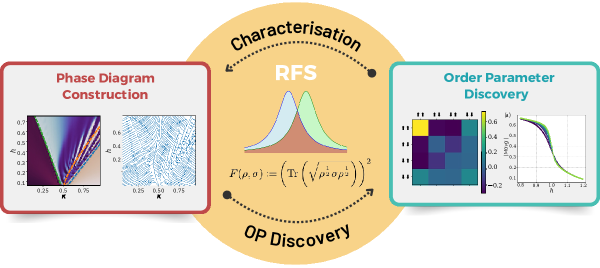
In this paper, we extend the use of the fidelity susceptibility from previous studies and construct a vector field using the reduced fidelity susceptibility (RFS). To this end, we characterize and detect different phases, specifically in the cluster Hamiltonian and Axial Next-Nearest Neighbor Ising (ANNNI) model [14, 15]. Not only does this approach allow us to demonstrate the proposed method, but also captures intricate details, such as the structure of ANNNI’s floating phase. A schematic picture of our method can be seen in Figure 1. Furthermore, we explore whether it is possible to identify an order parameter from a given Hamiltonian that accurately captures the phase transitions of a quantum system. Using the ANNNI model as an example, we provide a mathematical framework that enables the discovery of new order parameters for a model Hamiltonian, facilitating the understanding of different phases.
Finally, we note that our method can provide efficient certification and verification processes for quantum simulations and phase transition detection [16] and circumvents the need for full tomography of the wave-function, relying instead on reduced density matrix to capture the relevant characteristics thermodynamic information.
The outline of the paper is as follows. In Section II we outline the notation used in the paper and introduce the concept of fidelity and the RFS. This is followed by Section III, where we outline the mathematical framework, introduce the RFS vector field, and highlight its potential to be used to detect phase transitions. In Section IV, we highlight how the aforementioned mathematical framework can be used to determine an order parameter for a given quantum system. We showcase this in Section V by using the above framework to construct the phase diagram for both the ANNNI and cluster Hamiltonians and demonstrate the ability to discover new order parameters. We end with a discussion of applications of this framework in Section VI and potential use cases for future work.
II Preliminary
We begin by defining the set of Hermitian matrices of order , which is denoted by . We denote the identity matrix of order by and the th canonical basis vector for the vector space by .
Next, we introduce the concept of fidelity. Fidelity is a measure of the similarity between two quantum states and all its definitions embody the probability of distinguishing one quantum state from another.
Given mixed-states we define the Uhlmann-Jozsa fidelity [10] by111Some literature defines the fidelity in (1) as the square root of our (e.g. [17]).
| (1) |
which, for the remainder of the work, will be referred to as fidelity, unless otherwise specified. The latter definition of fidelity is not unique, indeed Jozsa [10] obtained an axiomatic definition for a family of such functions. However, the Uhlmann fidelity stands for its unique relation to the Bures distance
| (2) |
which is a quantification of the statistical distance between density matrices. A relevant result is the Uhlmann theorem [18], which expresses the fidelity in terms of the maximum overlap over all purifications of its arguments, that is
| (3) |
where and denote some purifications of and , respectively.
Following our discussion on the fidelity, we next consider a generic many-body parametric Hamiltonian , with eigenvalue equation , where the index identifies the ground state. In a perturbative approach w.r.t. a small parameter , the Taylor expansion for the fidelity reads
| (4) |
with the leading term (second-order) revealing the Fidelity susceptibility (susceptibility for short) [13]. We note that the first-order term vanishes since the fidelity reaches a maximum at for any . Informally, fidelity susceptibility quantifies how much the fidelity (or overlap) between two nearby states changes concerning a small change in a parameter (such as an external field or coupling strength) that defines the states. Let be the density matrix for the ground state of . Two well-known formulations for the susceptibility222The rightmost of (5a) is obtained by considering the Taylor expansion of , with from (4). are given as;
| (5a) | ||||
| (5b) | ||||
The expansion for the ground state of the perturbed Hermitian333This result is commonly known as the Rayleigh–Schrödinger perturbation theory [19]. reads
| (6) |
where . The latter leads to another well-known formulation for the susceptibility
| (7) |
As noticed in [20], the latter, which depends solely on the spectrum, shows that the quantity is non-negative and diverges when the energy gap closes.
III Phase Diagram Construction
Building upon the previous section’s exploration of fidelity susceptibility, we introduce the concept of the reduced fidelity susceptibility (RFS) vector field. In doing so, we consider a general many-body Hamiltonian parameterized by the space , of which its decomposition in terms of base and driving components reads
| (8) |
with control parameters . We anticipate that the choice of the two-dimensional parameters space is convenient for the visual approach, but not fundamental. Let denote the ground state of the Hamiltonian evaluated at , with denoting the underlying Hilbert space. The Hilbert space is assumed bipartite, that is , for some subsystems and . In addition, we assume the ground state is non-degenerate. Let denote the reduced density matrix (RDM) resulting from tracing out the subsystem for the ground state, so
| (9) |
We consider a perturbative action in the parameter space and define
| (10) |
for and a perturbation in the latter space, where is the fidelity defined in (1). As a consequence of the Uhlmann theorem (3), since the fidelity is the maximum over the overlap w.r.t. all purifications, then , that is the quantity in (10) is bounded below444Alternatively, this can be inferred by casting the partial trace as Kraus operator and by the monotonicity of the Uhlmann Fidelity [21]. by the square root of the overlap between the perturbed ground states.
Following this, we introduce one of the key functions for our method555 Interestingly, we can obtain another function proportional to that in (11) by considering defined in terms of the squared Bures distance (2). , that is
| (11) |
We call the terms the reduced fidelity susceptibility for the corresponding parameter . The adjective reduced is justified by the fact that we are considering RDMs instead of pure states as in (4). Similar forms of susceptibility have been considered in [22, 23]. As for the regular susceptibility, it is clear that the linear term in the perturbative Taylor expansion of vanishes for .
We next obtain the vector field (under sufficient smoothing assumptions, see details in subsection C.1) with rule
| (12) |
We stress that the gradient in (12) is expressed w.r.t. (parameters vector), whereas the Laplacian in (11) is related to (perturbation). In addition, we obtain a scalar function mapping the parameters to the angles of the vectors in the image of , that is
| (13) |
with denoting the principal argument666, with .. The latter is defined on the subset of the parameter space .
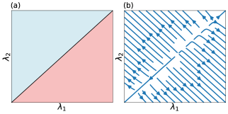
The function defined in (11) corresponds to a notion of fidelity susceptibility. Moreover, the angle given by in (13), is the direction of maximum decreasing of the susceptibility. Consequently, we expect that phase transitions materialize as sources in the vector field . An example of this can be seen in Figure 2. Furthermore, we note that the sinks are the points where the susceptibility reaches the local minimum. As the last step, if we map the co-domain of to a cyclic color map we expect to obtain the phase diagram of the Hamiltonian in (8). This process is illustrated in Figure 2, where we plot the principal argument. At the phase transition, a significant shift is observed as the value changes abruptly.
The practical implementation of the construction is expanded in Appendix A while in subsection C.1 we argue on the differentiability of the fidelity.
IV Order parameter discovery
Following the results obtained in the preceding section, we next investigate whether it is possible to determine the order parameter that captures the phase transitions of a given Hamiltonian.
To answer this question, we apply the protocol as described in Section III, and move from susceptibility-based identification of phases to determining the optimal observable for distinguishing the phases, that is a local order parameter. A simpler method has been proposed in [24], where a Hermitian operator is optimized to distinguish two given RDMs. In the latter, the distinction is given by the sign of the expectation w.r.t. the optimal observable. Our contribution instead, aims at mimicking the behaviour of order parameters.
We first note that the function in (13) represents the point-wise angle of the vector field (12). Also as argued before, phase transitions are likely to materialize as sources, and we assume that adjacent phases are distinguished by radian angles. In other words, if the parameter is proximal to a critical point (for some Hamiltonian), and a perturbation in the same space, then the assumption is that the corresponding gradient vectors have opposite directions, that is . Consequently, there exists an optimal angle such that
| (14) |
Consider a parametric Hamiltonian on spins with ground state RDM defined as in (9). Given a finite set of parameters in the neighbour of , we define a label for each parameter as . From (14), we see that distinct phases will be assigned opposite signs, . We define the index sets and , partitioning the indices for the parameters determining the ground states laying on the ordered and disordered phases, respectively. Under the assumption of non-degeneracy of the problem (see Appendix B for more details), we devise the following (non-convex) quadratically constrained quadratic program (QCQP) [25],
| s.t. | (15) |
with defining the expectation of at , and a tradeoff parameter. We denoted by the set of Hermitian matrices of order , which is also the order of the RDM .
This is commonly known in optimization literature as the trust region problem [26], which can be interpreted as a generalization of the minimum eigenvalue problem. The problem is solvable efficiently (polynomial time) even in the cases where the quadratic term is not positive semidefinite (i.e. non-convex) [27].
Informally, the optimization favors the non-zero expectation for the labels (ordered phase), whereas the quadratic term penalizes non-zero expectations for the labels (disordered phase). In essence, this mechanism is mimicking the order/disorder behavior of the order parameters. The choice of is sensible since extremal values or could render the problem degenerate (see Appendix B). The balance between the two expectation terms is regulated by the tradeoff parameter .
In practical terms, we consider RDMs on a few sites, thus the quadratic optimization problem can be solved classically upon computation of the partial trace on the ground states. Experimental results are presented in subsection V.2 and the details for the solution of the optimization are expanded in Appendix B.
Finally, we note, as given in [28] that the order parameter need not be unique, and any scaling operator that is zero in the disordered phase and non-zero in an adjacent (on the phase diagram), usually ordered phase, is a possible choice for an order parameter.
V Experiments
To demonstrate the potential of the fidelity vector field in identifying QPTs and their corresponding order parameters, we apply our above methods to the cluster Hamiltonian and ANNNI models.
V.1 The ANNNI model
We first focus on the ANNNI Model [29, 30, 15], a theoretical model commonly used in condensed matter physics to study the behavior of magnetic systems. The Hamiltonian of such a system can be written as
| (16) |
which we can rewrite in terms of the dimensionless ratios and . The former is called the frustration parameter while the latter is related to the transverse magnetic field.
In this model, spins are arranged in a one-dimensional lattice, with each spin existing in either the or state. The inclusion of the nearest neighbor and next-nearest-neighbor interactions in this model introduces a type of frustration, where the optimal alignment of neighboring spins is hindered due to competing interactions. The transverse field present, which represents an external magnetic field perpendicular to the direction of the spins, also induces quantum effects and modifies the overall behavior of the system. It is the combination of these complex interactions, which combine the effect of quantum fluctuations (owing to the presence of a transverse magnetic field) and frustrated exchange interactions that lead to phenomena such as quantum phase transitions. As a consequence, it is a paradigm for the study of competition between magnetic ordering, frustration, and thermal disordering effects [31].
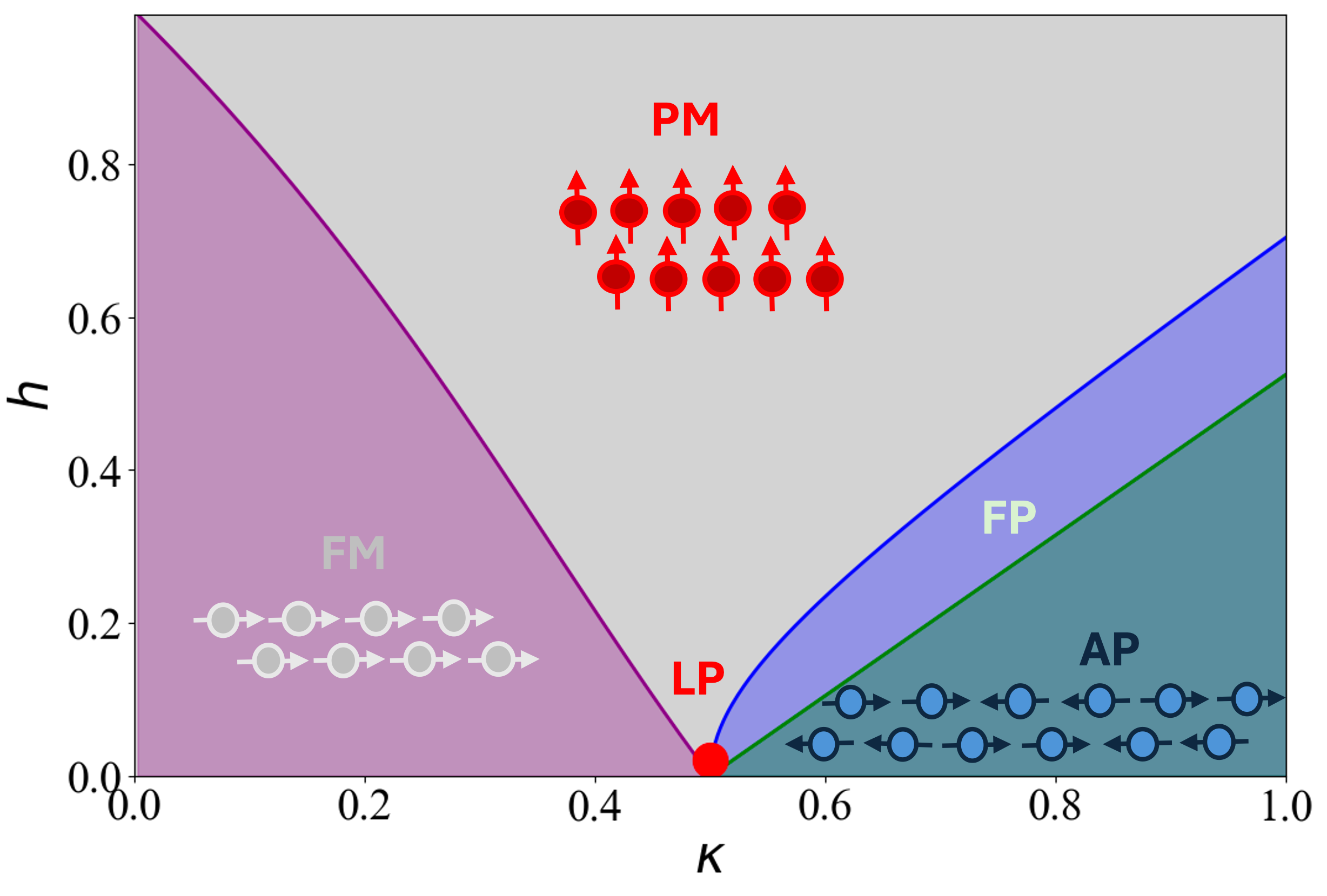
In the phase diagram shown in Figure 3, three distinct phase transitions are observed. The first transition is an Ising-like transition between the ferromagnetic (FM) and paramagnetic (PM) phases. The second is a Kosterlitz-Thouless (KT) transition that occurs between the paramagnetic and floating phase (FP). The final transition is the Pokrovsky-Talapov (PT) transition, which separates the floating phase (FP) from the antiphase (AP).
For more information regarding each of these phases and the corresponding phase transitions and their ground states see Appendix F.
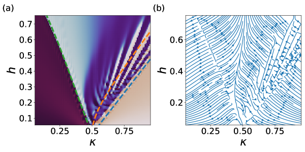
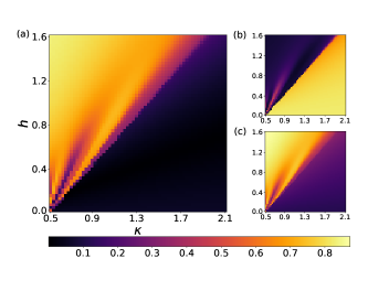
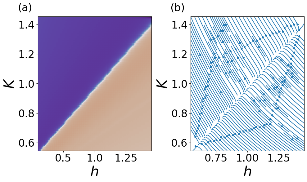
Using the formalism as outlined in Section III, we first obtain the ground states of the Hamiltonian using the density matrix renormalization group (DMRG). For details on how the RDM was obtained or the DMRG algorithm, see Appendix D. Next, we consider a two-site RDM and calculate the RFS vector field and its corresponding angles. In Figure 4 (a), we plot the angle as given in (13) of the RFS vector field, as well as the theoretical Ising, KT, and PT phase transition lines, given in green, orange and blue respectively. We note there is a noticeable overlap between the theoretical phase transition lines and the angle values, with the angle of the vector fidelity abruptly changing at each phase transition. Comparing the theoretical phase transition lines to the vector field plotted in Figure 4 (b), we observe that a source in the vector field indeed corresponds to a phase transition.
Additionally, it is worth noting that the fidelity vector field surpasses previous simulations in its ability to capture intricate details that were previously unresolved in the floating phase [32]. Distinct scar-like features are present, with the sources of the vector field corresponding to each of these structures indicating the presence of the phase transition between the paramagnetic and floating phases, specifically the KT transition. Future work will aim to explore the structure and fully utilize the potential of the RDS vector field in analyzing such complex phenomena. In the subsequent section, we demonstrate how we apply this method to determine order parameters for a given quantum system.
V.2 Order parameters discovery
Next, we experimentally demonstrate the validity of the method used for order parameter discovery (Section IV), and in doing so, propose a method for understanding the structure of the optimal observable. We proceed with the ANNNI model (16) by considering the phase diagram in the region and begin with the use of the RDMs of single spin sites. Let denote the optimal observable for the order parameter discovery problem in (IV), where the details concerning its solution are expanded in Appendix B. Optimizing for a single site observable, we find that , which can be interpreted as magnetization.
Although this observable could serve as an order parameter for the Ising-like transition, marked in green in Figure 4, it fails to detect the other transitions in the ANNNI model, namely the KT and PT transitions, which are highlighted in orange and blue, respectively, in Figure 4. Consequently, to identify all the phase transitions, one must refer to Section IV and instead develop a multi-site observable that can capture all the transitions.
For this, we expand our RDM to the two middle spin sites of the chain of length . The objective is to obtain the order parameters for the paramagnetic and the anti phases, which is highlighted in Figure 4, where we plot the result for the phase diagram construction (Section III) concerning the region , of which was obtained in the previous section using the RDS vector field.
In Figure 5 (a) we present the expectations of the observable applied to the RDMs , for a finite lattice of parameters , following the optimization process of obtaining a relevant order parameter for this phase transition. We note that in the optimization process, the entire region, , was used, which included all phase transitions present. Various values of in (IV) ranging from were also used, and it was found to have little effect in detecting each phase transition.
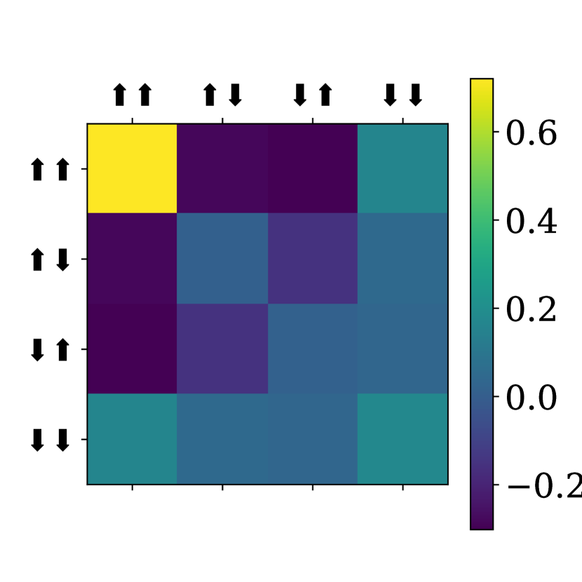
To understand the structure of the obtained observable, we next perform the eigendecomposition of , that is
| (17) |
where are rank-1 projectors and the corresponding eigenvalues. Let , we define the parametric Hermitian as
| (18) |
Such an operator can be interpreted as the orthogonal projector (which is defined as a square matrix such that generated by the state , where the angles of the spins are and , respectively.
The component corresponding to the eigenvalue with the greatest magnitude is the projector with and , that is . In Figure 5 (c), we plot the expectation of the observable . A comparison with the plot in Figure 5 (a), shows that this is the main component for the paramagnetic phase.
The component , with depicted in Figure 5 (b), can be interpreted as the complementary to . The operator approaches the following form
| (19) |
with (Bell’s state), so the ordered phase for is the antiphase. This can be justified by the modulated structure of the antiphase (see Appendix F for a comprehensive introduction to ANNNI). Indeed we see that for and , whereas (paramagnetic).
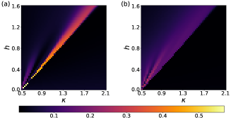
The remaining two components of the decomposition in (17) reveal an interesting structure. The third eigenvector determines the projector with and . Its expectation depicted in Figure 6 (a), appears to highlight a section of the floating phase. The last projector , whose details are omitted, produces another detail of the floating phase, which is depicted in Figure 6 (b).
V.3 Finite Size Scaling
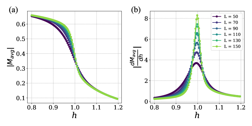
Next, we validate that the obtained observable is indeed an order parameter for the ANNNI Model. We accomplish this by applying finite-size scaling and verifying that the critical exponents match those expected for the Ising-like universality class. Finite-size scaling is a technique used to study phase transitions by examining how physical quantities change with system size. It involves scaling the system size and observing how properties such as critical exponents converge to their thermodynamic limits as the size increases. By applying this method, we can extrapolate results obtained from finite systems to infer behavior in the infinite system limit. To demonstrate this phenomena we thus analyze the impact of chain length at the Ising-like transition. We again use the RDM for two spin sites, which are related to the sites , assuming (linear size) is an even positive integer. We calculate the expectations of the observable with the reduced density matrices with and . In this parameter range, we can consider the next-nearest-neighbor interaction as a perturbation of the Ising model. Consequently, we anticipate observing the critical exponents characteristic of the 1D quantum Ising model.
If the observable indeed functions as an order parameter, it should satisfy the following scaling relation for the chain length [33]:
| (20) |
where and are constants, and represents the exponent of an irrelevant parameter.
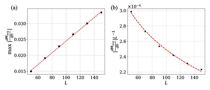
For the 1D quantum Ising model, where , the maximum of the gradient should show a linear dependence on the chain length. To validate this, we plot the maximum gradient as a function of the chain length, as shown in Figure 8. The observed linear relationship confirms that .
We then proceed to determine the irrelevant parameter exponent and show that this exponent remains positive as the chain length increases. Consequently, for large values of , the contribution from this term becomes negligible. As , this term approaches zero, leaving us with the critical exponents of the Ising model.
We first rescale the function such that and using gradient descent we fit for and . This fitting process is illustrated in Figure 8, where we plot . For irrelevant terms, we expect additional contributions to decay as increases, which is indeed observed in Figure 8. By applying gradient descent to the obtained expectations for various lengths, we determine and . Consequently, the positive value of the correction term confirms that it is an irrelevant parameter.
This analysis was also performed for the single-site observable , and the critical exponent was consistently obtained. Therefore, near the Ising transition, it retains the critical exponents characteristic of the Ising model, accounting for finite-size scaling correction terms. Based on this analysis, we conclude that the obtained observable functions as an order parameter.
V.4 The cluster Hamiltonian
After constructing the phase diagram for the ANNNI model, we will now showcase the versatility of the fidelity vector field method by applying it to other models. Specifically, we apply the method described in Section III to the cluster Hamiltonian, defined by the Hamiltonian:
| (21) |
When the two parameters of the Hamiltonian are equal we expect a phase transition between a trivial phase () and the Symmetry Protected Topological (SPT) phase (). To obtain the ground states of the Hamiltonian, we use DMRG, as described in Appendix D and we repeat the calculations as outlined in subsection V.1 to construct the phase diagram for the cluster Hamiltonian, of which is shown in Figure 9.
To conclude this section, we have demonstrated that the RFS vector field accurately reproduces the phase diagrams of both the ANNNI and cluster Hamiltonians, showcasing its robustness and reliability in capturing the phase transitions of diverse systems.
VI Conclusion
In conclusion, we have introduced a novel mathematical tool for detecting phase transitions in quantum systems through reduced fidelity susceptibility. Our analysis of the ANNNI model illustrates the tool’s capability to capture intricate phase transition details that were previously overlooked by conventional methods. This advancement not only highlights the potential for applying our framework to other models where phase transitions are either not well understood or not yet identified but also underscores its broader applicability and capacity for providing deeper insights into complex quantum systems.
Additionally, our framework demonstrates significant promise for application in quantum hardware environments. Utilizing the reduced density matrix thermodynamic information, it circumvents the need for full-function tomography while still capturing essential characteristics of phase transitions.
Moreover, we extended our framework to devise a method for discovering order parameters in systems where they are unknown. The reversed method, applied to the ANNNI model, was validated through the decomposition and finite-size scaling of the identified order parameter. This validation underscores the framework’s potential to explore and analyze novel systems, including unexplored phenomena such as floating phases in a quantum system. We believe that the proposed approach is an important milestone in phase transition detection and order parameter discovery, offering a robust tool for exploring the complex landscape of quantum systems.
VII Acknowledgment
We are grateful to Dmytro Mishagli (IBM) and Victor Valls (IBM) for their valuable input and suggestions.
F.DM and E.R. acknowledge support from the BasQ strategy of the Department of Science, Universities, and Innovation of the Basque Government.
E.R. is supported by the grant PID2021-126273NB-I00 funded by MCIN/AEI/ 10.13039/501100011033 and by “ERDF A way of making Europe” and the Basque Government through Grant No. IT1470-22. This work was supported by the EU via QuantERA project T-NiSQ grant PCI2022-132984 funded by MCIN/AEI/10.13039/501100011033 and by the European Union “NextGenerationEU”/PRTR. This work has been financially supported by the Ministry of Economic Affairs and Digital Transformation of the Spanish Government through the QUANTUM ENIA project called – Quantum Spain project, and by the European Union through the Recovery, Transformation, and Resilience Plan – NextGenerationEU within the framework of the Digital Spain 2026 Agenda.
Appendix A Construction of the phase diagram
Starting from results devised in Section III, we proceed with the numerical construction of the phase diagram. We consider a rectangular region of the Hamiltonian parameters . Given a step in the parameters space , we construct a finite lattice of parameters , such that
| (22) |
with belonging to a subset of . Using the density matrix renormalization group (DMRG) [34, 35], we obtain the RDM related to the ground state (for a selected subsystem) for the parameter , which we define as , where the RHS is defined in (9). In Figure 10 the lattice points for the RDMs are represented by the symbol .
We proceed with the preparation of an approximation of the function , that is the RFS defined in (11). The latter is the Laplacian of the function defined in (10). So, starting from the lattice of parameters , we obtain the fidelity perturbations
| (23) |
for a fixed step (which defines the lattice of parameters) and . We can immediately verify the computational advantage of the approach since adjacent lattice points share a fidelity perturbation. For example . In Figure 10, the fidelity perturbations are represented with the symbol and placed between adjacent lattice points to emphasize the concept of sharing. By considering the finite differences approximation of the second derivative777 For a function , under sufficient smoothing conditions, we make use of the following approximation (24) for some . , and by noting that (for all valid ), we obtain
| (25) |
where is the set of perturbation displacements around . In practice, we omit the factor (numerically convenient) which is irrelevant for the subsequent computations. We proceed by adhering to the structure outlined in Section III. Obtained the RFS approximation , we continue with the computation of its gradient. Before that, we need to introduce a few concepts related to discrete signal processing.
For a continuous function , we define the convolution at for discrete 2-dimensional signals as
| (26) |
where is a convolution kernel with support , that is for or . Also, the scalar represents the step for the lattice of points . We introduce a discrete differentiation operator called the Sobel operator [36] whose component is given by the kernel matrix
| (27) |
The Sobel finds applications mainly in computer vision and it was initially developed to obtain an efficiently computable gradient operator with more isotropic characteristics than the Roberts cross operator [37].
Now, we define our kernel as , which corresponds to the approximation of the gradient w.r.t. on the real part and the component on the imaginary part.
We obtain an equivalent approximation of in (12) using the convolution
| (28a) | ||||
| (28b) | ||||
When the indices of the lattice elements are beyond the limits of definition we define .
The first outcome of the process is a point-to-color graph
| (29) |
where is a colormap which we introduce now. Let be a space of colors and let be a mapping from the angle to a color in . The function is required to be smooth on and non-constant, also it must be such that . The latter point is fundamental for dealing with the discontinuity of in the non-positive real axis. Colormaps fulfilling the latter conditions are known as cyclic [38, 39]. In addition, the resulting signal is upsampled by factor 2 using an interpolation filter [40]. An example outcome obtained using the present procedure is reported in Figure 4.
The final step of the diagram construction consists of the plotting of the vector field in (12).
The approach makes use of the Runge–Kutta method [41] and our reference implementation is part of the function
matplotlib.pyplot.streamplot of the software package Matplotlib [39].
In the realm of differential equations, the Runge–Kutta method is a well-known algorithm for solving initial-value problems.
In our instance, the velocities on the lattice are given by the gradient in (12).
The initial values instead, are the points on the boundary of the lattice.
Furthermore, a heuristic path of lattice points spiraling toward the center is added to the initial values, to improve the density of the streamlines.
Appendix B Solution of the order parameter discovery problem
In this section, we expand on the solution of the order parameter discovery problem defined in (IV). We restate the latter for clarity and convenience, so
| s.t. | (30) |
with .
We introduce the row-major vectorization operator defined as
| (31) |
for any matrix of order in . For matrices of order we will be using the identity
| (32) |
We recall that we denoted the set of Hermitians of order in . We define the set of vectorized Hermitians of order as
| (33) |
Assuming , for some finite index set , we note that
| (34a) | ||||
| (34b) | ||||
| (34c) | ||||
with and . We note that the vectors and belong to .
We use the result in (34a) to rewrite the optimization problem in (IV) as
| (35a) | ||||
| s.t. | (35b) | |||
| (35c) | ||||
with
| (36) |
The matrix (determined by data) is Hermitian, so the objective in (35a) is real and well-defined (even in the absence of constraint (35c)). We expand on the condition for the non-degeneracy of the problem introduced in Section IV. We impose that the matrix is indefinite [42], where the Hermitian structure is fulfilled by the construction in (36). In other words, we require the matrix to have both (strictly) positive and negative eigenvalues. The construction of shows the difference between two PSDs, so the tradeoff is a sensible parameter since it can render the problem (numerically) degenerate.
Let denote the Loewner order [42], that is the partial order on the cone of PSD matrices. Specifically, for any pair of PSD matrices we have that if and only if is PSD.
The optimization problem is non-convex since we do not assume , indeed is required indefinite. However, as anticipated in Section IV, this optimization problem can be solved efficiently even in the case of the non-convexity of the objective (i.e. matrix is not PSD). Moreover, this is an exceptional case where strong duality888 Strong duality is equivalent to the duality gap is zero, that is the difference between primal and dual solutions. [25] holds, provided that Slater’s constraint qualification is fulfilled. That is, there exists an such that the inequality constraint (35b) holds strictly (i.e. not tight). In our case, an example is for any , so .
Now, we consider the optimization problem consisting of (35a) and (35b). We exclude the constraint in (35c), as we will prove being enforced implicitly by the structure of the matrix and the non-degeneracy conditions. The Lagrangian function is with the multiplier . Consequently, the dual function takes the value when (i.e. PSD, so the Lagrangian is bounded below in ), and it becomes unbounded otherwise. Let denote the minimum eigenvalue of the matrix argument. The Lagrange dual problem reads
| (37a) | ||||
| s.t. | (37b) | |||
then the constraint is fulfilled when , so the dual optimal is . The space of the primal solutions is given by the eigenspace corresponding to the minimum eigenvalue of , that is the null space of the latter. Given any matrix , we denote the null space of (i.e. the set of solutions of the homogeneous equation ) by . Let
| (38) |
with , be an optimal solution999 We note that the vectorization operator is an isomorphism, so the expression implicitly means that the matrix is obtained uniquely from using the inverse of . , we show that if , then . That is constraint (35c) is implied by the structure of matrix .
The set of Hermitian matrices of order is a real vector space, and if is a basis for it, then is a basis for the vector space of vectorized Hermitians. We verify immediately that, by construction, the image of matrix belongs to the latter vector space. By the non-degenerancy assumptions (i.e. is Hermitian indefinite), we have that . Consequently, the solution belongs to the image of , hence the matrix such that is Hermitian. In other words, we have shown that the assumption that is Hermitian indefinite implies that constraint (35c) is fulfilled. When the non-degeneracy conditions are not met, the case corresponds to the impossibility of obtaining an order parameter (which could be conditioned to the size of the observable). This is a situation we encountered in subsection V.2.
In (38) we have proved that the solution may not be unique, however, this is consistent with the non-uniqueness of order parameters stated in Section IV.
We note that even in the case of 1-dimensional null space in (38), the optimal observable can be of any rank since the solution is a vectorization of a Hermitian operator. For example, in the case of the Ising model, we could have (a Bell’s basis vector) with the corresponding observable being (full rank).
We summarize the procedure. Given a lattice of RDMs for the ground states of a selected Hamiltonian, we obtain the vector field in (12). The labeling of the phases is obtained using the trigonometric approach explained in Section IV, so we derive the sets and . Subsequently to the instantiation of matrix given in (36), we use its eigendecomposition to obtain, first, the verification that the non-degeneracy conditions are met. Secondly, the eigenspace corresponding to its minimum eigenvalue determines the space of solutions (38).
Appendix C Additional results
C.1 Discontinuities of fidelity and its susceptibility
We produce a counterexample which proves that the assumption on the non-degeneracy of the ground state (stated in Section III) is not sufficient to guarantee the continuity of fidelity when dealing with RDM. For example, consider a parametric state , with and , defined by the Schmidt decomposition [43]
| (39) |
with and denoting some bases for and , respectively. We obtain the RDM by tracing out the subsystem , so
| (40) |
It is clear that the parameter determines a change of rank of . In the case of a RDM acting on , the Uhlmann fidelity matches the formulation of the Superfidelity [44] which is defined as
| (41) |
Then considering , the rightmost term for the fidelity in (41) becomes
| (42) |
where is a constant depending on . We see that the resulting function of is discontinuous for . In other words, a tiny perturbation could cause a change of rank of and a loss of continuity (and so smoothness).
In practice, we do not know the locations in the parameters space where such phenomena could happen. However, the procedure of sampling and smoothing described in Appendix A can be interpreted as an implicit mollification. Consequently, the plot of the mollified vector field (for example Figure 4) should present sharp changes in direction, sources or sink in the proximity of such regions.
Appendix D Experimental Methods
To calculate the ground states for the reduced fidelity susceptibility, we use the density matrix renormalization algorithm (DMRG) [45]. We use two different software packages called Tensor Network Python TeNPy [35] and Quantum Simulation with MPS Tensor qs-mps [46].
For the ANNNI model we span the region while for the cluster . We take points for each axis resulting in a lattice of parameters, with a maximum bond dimension . Both Hamiltonians in the top-left corner of their respective regions are dominated by the term and thus the states will be a perturbation of the all-up state . To ensure the convergence of the DMRG calculations, we use the following strategy: We begin with a region where the states are relatively easy to prepare and where the DMRG converges reliably. From there, we extend the calculation to include nearest-neighbor lattice points, using the previously obtained state as the initial state. We continue this approach, gradually moving towards regions where states are more challenging to prepare. In doing so, we gain both accuracy and speed.
We note the most time consuming part of the calculation is solving the local eigenvalue problem through the method eigsh from the software package SciPy [47].
This procedure is effective up until the point of a phase transition. At that point, if the computation time exceeds a specified threshold (which can be set either arbitrarily or adaptively), we shelve the calculation and proceed to the next lattice point.
Appendix E Discovered Order Parameter of the ANNNI Model
Following the procedure given in Section IV for the ANNNI model, the two-site observable matrix is given in Figure 11 and decomposed in subsection V.2.
The decomposition of the observable in terms of Pauli Operators is given as follows;
Appendix F The ANNNI model
We first present the phase diagram for the ANNNI Model which is given in Figure 3, where a variety of rich phase transitions are present. We initially begin with small and , where the interactions between neighbors along the x-axis dominate, resulting in a ferromagnetic phase where all spins align parallel to one another, either as or . This ferromagnetic region is highlighted in purple in Figure 3.
Upon increasing and , a phase transition occurs as the spins enter a paramagnetic phase (PM), presented in grey in Figure 3. Entering the paramagnetic phase, the transverse magnetic field begins to dominate, causing all states to align with the magnetic field, resulting in the state . This Ising-like transition has been previously studied in [48] and the transition line (which corresponds to the purple line in Figure 3 is given in [8, 48] as;
| (43) |
Increasing the parameters and , a further transition becomes evident in the phase diagram between the paramagnetic and floating phases (FP). This incommensurate-incommensurate Kosterlitz-Thouless (KT) phase transition [49, 50, 51] (given in blue in Figure 3) has been approximated in [52] to be
| (44) |
Such a transition corresponds to a change in the modulation wave vector [53], leading to different incommensurate structures along the spin chain.
A further transition evident in this phase diagram is the transition from the floating phase to the antiphase (AP), where the states exhibit staggered magnetization, as a result of the next-nearest neighbor interactions dominating, corresponding to . Such an incommensurate-commensurate transition (given in green in Figure 3) is described by the Pokrovsky-Talapov universality class [49, 54], with the transition in this case given by
| (45) |
as highlighted in [52] and corresponds to the green line in Figure 3. We also note the presence of the Lifshitz point, marked by a red dot in Figure 3. This point represents a critical point, known as the Lifschitz point (LP), on the phase diagram of certain magnetic systems, where a line of second-order phase transitions meets a line of incommensurate modulated phases [55]. Lastly, we observe that the ANNNI model features a disorder line, known as the Peschel-Every (PE) line [56], which lies within the paramagnetic phase and provides a reference point for comprehending the properties of this particular phase.
Finally, we note this model also reproduces important features observed experimentally in systems that can be described by discrete models with effectively short-range competing interactions [15]. These experimental findings include Lifshitz points [57, 58], adsorbates, ferroelectrics, magnetic systems, and alloys. Conversely, the so-called floating phase emerging in the model is appealing to experimental researchers to explore. This critical incommensurate phase has been observed very recently by using Rydberg-atom ladder arrays [59].
References
- [1] V. L. Ginzburg and L. D. Landau. On the Theory of superconductivity. Zh. Eksp. Teor. Fiz., 20:1064–1082, 1950.
- [2] Leo Kadanoff, Alessandro de angelis, Nicola Giglietto, Sebastiano Stramaglia, M Kibler, and Dennis Dieks. Theories of matter: Infinities and renormalization. arXiv:1002.2985, 02 2010.
- [3] Leo P. Kadanoff. Relating theories via renormalization. Studies in History and Philosophy of Science Part B: Studies in History and Philosophy of Modern Physics, 44(1):22–39, 2013.
- [4] Humphrey J. Maris and Leo P. Kadanoff. Teaching the renormalization group. American Journal of Physics, 46(6):652–657, 06 1978.
- [5] Kerson Huang. A critical history of renormalization. International Journal of Modern Physics A, 28(29):1330050, 2013.
- [6] Vincent Ardourel and Sorin Bangu. Finite-size scaling theory: Quantitative and qualitative approaches to critical phenomena. Studies in History and Philosophy of Science, 100:99–106, 2023.
- [7] Saverio Monaco, Oriel Kiss, Antonio Mandarino, Sofia Vallecorsa, and Michele Grossi. Quantum phase detection generalization from marginal quantum neural network models. Physical Review B, 107(8), February 2023.
- [8] M. Cea, M. Grossi, S. Monaco, E. Rico, L. Tagliacozzo, and S. Vallecorsa. Exploring the phase diagram of the quantum one-dimensional annni model. arXiv:2402.11022, 2024.
- [9] Teresa Sancho-Lorente, Juan Román-Roche, and David Zueco. Quantum kernels to learn the phases of quantum matter. Phys. Rev. A, 105:042432, Apr 2022.
- [10] Richard Jozsa. Fidelity for mixed quantum states. Journal of Modern Optics, 41(12):2315–2323, 1994.
- [11] Amit Dutta, Gabriel Aeppli, Bikas K. Chakrabarti, Uma Divakaran, Thomas F. Rosenbaum, and Diptiman Sen. Quantum Phase Transitions in Transverse Field Spin Models: From Statistical Physics to Quantum Information. Cambridge University Press, 2015.
- [12] Shi-Jian GUu. Fidelity approach to quantum phase transitions. International Journal of Modern Physics B, 24(23):4371–4458, September 2010.
- [13] Wen-Long You, Ying-Wai Li, and Shi-Jian Gu. Fidelity, dynamic structure factor, and susceptibility in critical phenomena. Phys. Rev. E, 76:022101, Aug 2007.
- [14] Jiannis K. Pachos and Martin B. Plenio. Three-spin interactions in optical lattices and criticality in cluster hamiltonians. Phys. Rev. Lett., 93:056402, Jul 2004.
- [15] Walter Selke. The annni model — theoretical analysis and experimental application. Physics Reports, 170:213–264, 1988.
- [16] Jose Carrasco, Andreas Elben, Christian Kokail, Barbara Kraus, and Peter Zoller. Theoretical and experimental perspectives of quantum verification. PRX Quantum, 2:010102, Mar 2021.
- [17] Michael A. Nielsen and Isaac L. Chuang. Quantum Computation and Quantum Information: 10th Anniversary Edition. Cambridge University Press, USA, 10th edition, 2011.
- [18] Armin Uhlmann. The ”transition probability” in the state space of a *-algebra. Reports on Mathematical Physics, 9:273–279, 1976.
- [19] E. Schrödinger. Quantisierung als Eigenwertproblem. Annalen Phys., 384(4):361–376, 1926.
- [20] Lei Wang, Ye-Hua Liu, Jakub Imriška, Ping Nang Ma, and Matthias Troyer. Fidelity susceptibility made simple: A unified quantum monte carlo approach. Physical Review X, 5(3), July 2015.
- [21] Paulo E. M. F. Mendonça, Reginaldo d. J. Napolitano, Marcelo A. Marchiolli, Christopher J. Foster, and Yeong-Cherng Liang. Alternative fidelity measure between quantum states. Physical Review A, 78(5), November 2008.
- [22] Paolo Zanardi, H. T. Quan, Xiaoguang Wang, and C. P. Sun. Mixed-state fidelity and quantum criticality at finite temperature. Phys. Rev. A, 75:032109, Mar 2007.
- [23] Paolo Zanardi, Lorenzo Campos Venuti, and Paolo Giorda. Bures metric over thermal state manifolds and quantum criticality. Phys. Rev. A, 76:062318, Dec 2007.
- [24] Shunsuke Furukawa, Grégoire Misguich, and Masaki Oshikawa. Systematic derivation of order parameters through reduced density matrices. Phys. Rev. Lett., 96:047211, Feb 2006.
- [25] Stephen Boyd and Lieven Vandenberghe. Convex Optimization. Cambridge University Press, 2004.
- [26] Andrew R. Conn, Nicholas I. M. Gould, and Philippe L. Toint. Trust Region Methods. Society for Industrial and Applied Mathematics, 2000.
- [27] Franz Rendl and Henry Wolkowicz. A semidefinite framework for trust region subproblems with applications to large scale minimization. Mathematical Programming, 77(1):273–299, Apr 1997.
- [28] N. Goldenfeld. Lectures On Phase Transitions And The Renormalization Group. CRC Press, 1992.
- [29] R. J. Elliott. Phenomenological discussion of magnetic ordering in the heavy rare-earth metals. Phys. Rev., 124:346–353, Oct 1961.
- [30] Michael E. Fisher and Walter Selke. Infinitely many commensurate phases in a simple ising model. Phys. Rev. Lett., 44:1502–1505, Jun 1980.
- [31] Anjan Kumar Chandra and Subinay Dasgupta. Floating phase in a 2D ANNNI model. Journal of Physics A Mathematical General, 40(24):6251–6265, June 2007.
- [32] Anjan Kumar Chandra and Subinay Dasgupta. Floating phase in the one-dimensional transverse axial next-nearest-neighbor ising model. Phys. Rev. E, 75:021105, Feb 2007.
- [33] P.H. Lundow and I.A. Campbell. The ising universality class in dimension three: Corrections to scaling. Physica A: Statistical Mechanics and its Applications, 511:40–53, 2018.
- [34] U. Schollwöck. The density-matrix renormalization group. Rev. Mod. Phys., 77:259–315, Apr 2005.
- [35] Johannes Hauschild and Frank Pollmann. Efficient numerical simulations with Tensor Networks: Tensor Network Python (TeNPy). SciPost Phys. Lect. Notes, page 5, 2018. Code available from https://github.com/tenpy/tenpy.
- [36] Irwin Sobel. An isotropic 3x3 image gradient operator. Presentation at Stanford A.I. Project 1968, 02 2014.
- [37] Larry S. Davis. A survey of edge detection techniques. Computer Graphics and Image Processing, 4(3):248–270, 1975.
- [38] Peter Kovesi. Good colour maps: How to design them. arXiv:1002.2985, 2015.
- [39] J. D. Hunter. Matplotlib: A 2d graphics environment. Computing in Science & Engineering, 9(3):90–95, 2007.
- [40] F.J. Harris. Multirate Signal Processing for Communication Systems. Prentice Hall PTR, 2004.
- [41] J.C. Butcher. A history of runge-kutta methods. Applied Numerical Mathematics, 20(3):247–260, 1996.
- [42] Roger A. Horn and Charles R. Johnson. Matrix Analysis. Cambridge University Press, USA, 2nd edition, 2012.
- [43] Ingemar Bengtsson and Karol Zyczkowski. Geometry of Quantum States: An Introduction to Quantum Entanglement. Cambridge University Press, 2006.
- [44] J. Miszczak, Zbigniew Puchała, P. Horodecki, Armin Uhlmann, and Karol Zyczkowski. Sub– and super–fidelity as bounds for quantum fidelity. Quantum Information and Computation, 9, 06 2008.
- [45] Ulrich Schollwöck. The density-matrix renormalization group in the age of matrix product states. Annals of Physics, 326(1):96–192, January 2011.
- [46] Francesco Di Marcantonio. Quantum simulation with mps tensor, 2024. Code available from https://github.com/Fradm98/qs-mps.
- [47] Pauli Virtanen, Ralf Gommers, Travis E. Oliphant, Matt Haberland, Tyler Reddy, David Cournapeau, Evgeni Burovski, Pearu Peterson, Warren Weckesser, Jonathan Bright, Stéfan J. van der Walt, Matthew Brett, Joshua Wilson, K. Jarrod Millman, Nikolay Mayorov, Andrew R. J. Nelson, Eric Jones, Robert Kern, Eric Larson, C J Carey, İlhan Polat, Yu Feng, Eric W. Moore, Jake VanderPlas, Denis Laxalde, Josef Perktold, Robert Cimrman, Ian Henriksen, E. A. Quintero, Charles R. Harris, Anne M. Archibald, Antônio H. Ribeiro, Fabian Pedregosa, Paul van Mulbregt, and SciPy 1.0 Contributors. SciPy 1.0: Fundamental Algorithms for Scientific Computing in Python. Nature Methods, 17:261–272, 2020.
- [48] Sei Suzuki, Jun-ichi Inoue, and Bikas K. Chakrabarti. Quantum Ising Phases and Transitions in Transverse Ising Models, volume 859. 2013.
- [49] V. L. Pokrovsky and A. L. Talapov. Ground state, spectrum, and phase diagram of two-dimensional incommensurate crystals. Phys. Rev. Lett., 42:65–67, Jan 1979.
- [50] David A. Huse and Michael E. Fisher. Commensurate melting, domain walls, and dislocations. Phys. Rev. B, 29:239–270, Jan 1984.
- [51] P. Bak. Review Article: Commensurate phases, incommensurate phases and the devil’s staircase. Reports on Progress in Physics, 45(6):587–629, June 1982.
- [52] Matteo Beccaria, Massimo Campostrini, and Alessandra Feo. Evidence for a floating phase of the transverse annni model at high frustration. Phys. Rev. B, 76:094410, Sep 2007.
- [53] Ruben Verresen, Ashvin Vishwanath, and Frank Pollmann. Stable Luttinger liquids and emergent symmetry in constrained quantum chains. arXiv e-prints, page arXiv:1903.09179, March 2019.
- [54] Y.-J. Wang, F. H. L. Essler, M. Fabrizio, and A. A. Nersesyan. Quantum criticalities in a two-leg antiferromagnetic ladder induced by a staggered magnetic field. Phys. Rev. B, 66:024412, Jul 2002.
- [55] A.K. Murtazaev and J.G. Ibaev. Critical properties of an annni-model in the neighborhood of multicritical lifshitz point. Solid State Communications, 152:177–179, 02 2012.
- [56] I Peschel and V J Emery. Calculation of spin correlations in two-dimensional ising systems from one-dimensional kinetic models. Zeitschrift für Physik B Condensed Matter, 43(3):241–249, September 1981.
- [57] Malte Henkel and Michel Pleimling. Lifshitz Points: Strongly Anisotropic Equilibrium Critical Points, pages 337–368. Springer Netherlands, Dordrecht, 2010.
- [58] R.M. Hornreich. The lifshitz point: Phase diagrams and critical behavior. Journal of Magnetism and Magnetic Materials, 15-18:387–392, 1980.
- [59] Jin Zhang et al. Probing quantum floating phases in Rydberg atom arrays. arXiv: 2401.08087, 1 2024.