Anderson localization of light by impurities in a solid transparent matrix

Abstract

A solid transparent medium with randomly positioned, immobile impurity atoms is a promising candidate for observation of Anderson localization of light in three dimensions. It can have low losses and allows for mitigation of the detrimental effect of longitudinal optical fields by an external magnetic field, but it has its own issues: thermal oscillations of atoms around their equilibrium positions and inhomogeneous broadening of atomic spectral lines due to random local electric fields. We show that these complications should not impede observation of Anderson localization of light in such materials. The thermal oscillations hardly affect light propagation whereas the inhomogeneous broadening can be compensated for by increasing the number density of impurity atoms.

Anderson localization—a complete halt of wave transport due to disorder [1]—turns out to be difficult [2, 3, 4, 5, 6, 7, 8, 9, 5, 10, 11] and likely even impossible [12] to reach for light in fully disordered three-dimensional (3D) dielectric media. Partially ordered structures such as disordered photonic crystals [13, 14, 15] or hyperuniform materials [16, 17] featuring a photonic band gap may be required to obtain spatially localized optical modes at frequencies near a band edge where the optical density of states is strongly suppressed. Metallic structures may be better suitable for observation of Anderson localization of light than dielectric ones [18, 12] although real metals suffer from significant losses that can make optical experiments difficult to conduct and interpret [18, 19].

Cold atoms exhibiting purely elastic, lossless scattering have been proposed as an alternative medium for observation of Anderson localization of light in 3D without relying on photonic band gap effects [20, 21]. However, longitudinal electric fields have been later predicted to prevent such an observation [22, 23]. A possible solution to this problem consists in placing the atoms in a strong external magnetic field that partially suppresses longitudinal fields [24, 25]. Theoretical work has predicted the expected signatures of Anderson localization for coherent laser light in optically thick and dense cold-atom ensembles placed in a strong external magnetic field: slowing down of the temporal decay of a transmitted pulse [26], enhanced fluctuations of scattered intensity [27], step-like profile of average intensity inside the atomic sample [28]. However, the experimental realization of these theoretical predictions is currently impeded by the following two main obstacles. First, it is difficult to prepare cold-atom samples that would be optically thick to ensure multiple scattering (size $L>$ photon mean free path $\ell$) and, at the same time, sufficiently dense to reach Anderson localization (atomic number density $\rho>\lambda_{0}^{-3}$, where $\lambda_{0}$ is the resonance wavelength in the free space) [29, 21]. Second, experiments are necessarily performed at a low but finite temperature (typically, $T\sim 100$ $\mu$K [29, 30]) leading to residual motion of atoms that is likely to wash out interference phenomena in general and Anderson localization in particular [26, 31].

A transparent solid medium with impurity atoms or ions embedded at random locations is an alternative physical system described by the theoretical model of immobile point-like scattering centers (atoms or ions) developed in Refs. [22, 23, 24, 26, 25] and exhibiting the phenomenon of Anderson localization. Well-known examples of such materials are uranium glass (with U atoms in, e.g., oxide diuranate form as impurities) [32] and ruby (with Cr³⁺ ions as impurities), for which the possibility of Anderson localization of optical excitations have been already evoked [33, 34]. Another example is the diamond crystal with multiple nitrogen-vacancy centers—a system with promising application in quantum information science [35, 36]. Such media have a number of advantages as compared to cold atomic gases as far as the observation of Anderson localization of light is concerned. On the one hand, they can be found in nature or fabricated without fundamental limitations on the medium size $L$ or impurity number density $\rho$, so that the conditions $L>\ell$ and $\rho>\lambda_{0}^{-3}$ can be readily fulfilled. On the other hand, experiments can be performed at room or, in any case, not-too-low temperature because impurities are fixed at their positions in the matrix and do not fly away. Two problems arise nevertheless in these systems. First, local electric fields induce position-dependent shifts of resonance frequencies of impurity atoms, driving them out of resonance with each other. Such an inhomogeneous broadening of the spectrum is expected to reduce the maximum achievable scattering strength, which may bring the system away from the Anderson localization regime. Second, the problem of atomic motion that is crucial in atomic gases, does not disappear completely here either: the solid matrix still allows for oscillations of impurity atoms about their equlibrium positions with an amplitude and a frequency determined by the temperature. At the first glance, such oscillations could be expected to be less detrimental for Anderson localization of light than the free atomic motion, but it is not clear to which degree. Thus, it is not clear a priori whether the replacement of free atomic motion by oscillations brought about by embedding the atoms in a solid host medium overweighs the detrimental impact of random local fields due to the very same host medium and makes Anderson localization achievable under realistic conditions.

In the present Letter we analyze a theoretical model including both the oscillations of impurity atoms about their equilibrium positions and random frequency shifts of atomic energy levels. Our analysis predicts that Anderson localization of light should be achievable in random ensembles of impurity atoms embedded in a transparent solid host medium at finite temperatures. In particular, the fast but small-amplitude oscillations of impurity atoms around their equilibrium positions have virtually no effect on light propagation, in analogy with Dicke narrowing of Doppler broadened spectral lines in the presence of atomic collisions [37]. In contrast, the inhomogeneous broadening of atomic spectral lines does suppress scattering and makes Anderson localization more difficult to reach. However, this suppression can be compensated by increasing the number density of atoms, so that a photon mobility edge always exist, whatever the broadening.

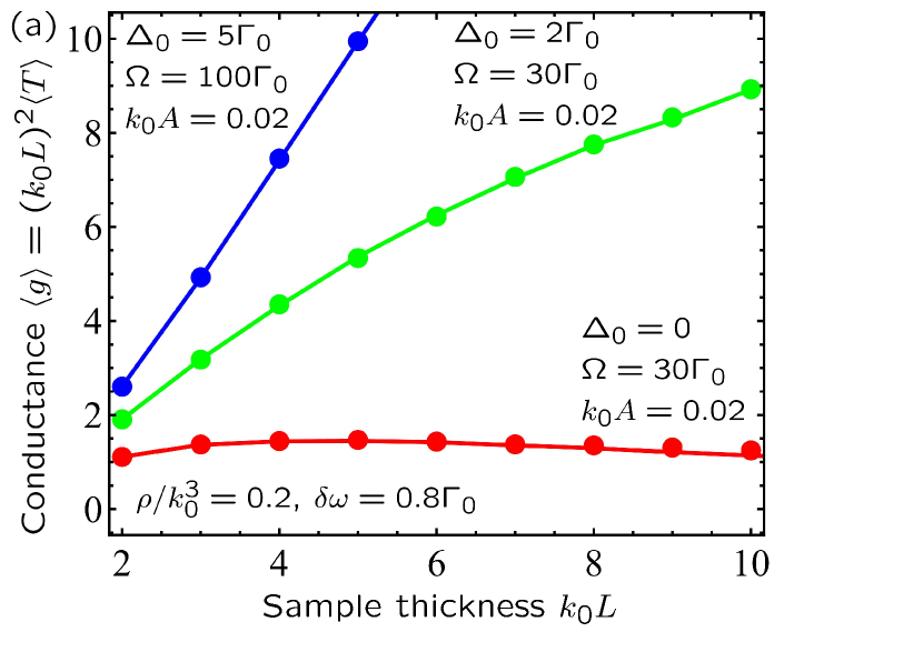
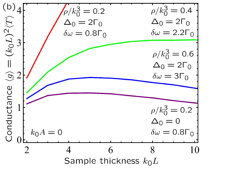
Figure 1: Average dimensionless conductance $\langle g\rangle$ as a function of sample thickness $L$, for different parameters. Full circles result from full dynamic calculations taking into account fast oscillations of impurity atoms around random equilibrium positions with frequency $\Omega$ and amplitudes $A_{n\mu}\sim{\cal{N}}(0,A)$, as well as random frequency shifts of impurity resonant frequencies $\Delta_{n}\sim{\cal{N}}(0,\Delta_{0})$. Solid lines are obtained by neglecting oscillations ($A=0$).

We start with a standard Hamiltonial $\hat{H}$ describing the free electromagnetic field coupled with $N$ identical two-level atoms located at positions $\{{\mathbf{r}}_{n}\}$ and having each a ground state $|g\rangle$ with energy $E_{g}$ and angular momentum $J_{g}=0$, three degenerate excited states $|e_{m}\rangle$, $m=0,\pm 1$, with energy $E_{e}=E_{g}+\hbar\omega_{0}$ and angular momentum $J_{e}=1$, and the dipole moment ${\mathbf{d}}_{e_{m}g}$ of the transition $|g\rangle\to|e_{m}\rangle$ [38, 39]. Symmetry considerations impose $|{\mathbf{d}}_{e_{m}g}|=d$ independent of $m$. We follow the now well-known procedure to eliminate field variables and obtain an effective non-Hermitian Hamiltonian $\hat{H}_{\text{eff}}$ describing immobile atoms coupled by the quasi-resonant electromagnetic field [40, 41]. When the lifting of the degeneracy of the excited state by an external magnetic field ${\mathbf{B}}=B{\mathbf{e}}_{z}$ and the inhomogeneous broadening of atomic spectral lines $\omega_{n}=\omega_{0}+\Delta_{n}$ are included in the model, the effective Hamiltonian is composed of $N\times N$ blocks of size $3\times 3$ that in units of $\hbar\Gamma_{0}/2$ can be written as

$$\begin{aligned} \left(\hat{H}_{\text{eff}}\right)_{nn^{\prime}}&=\left[\left(i-\frac{2\Delta_{n}}{\Gamma_{0}}\right)\mathbb{1}-\frac{2\Delta_{B}}{\Gamma_{0}}\begin{pmatrix}-1&0&0\\ 0&0&0\\ 0&0&1\end{pmatrix}\right]\delta_{nn^{\prime}}\\ &-\frac{6\pi}{k_{0}}(1-\delta_{nn^{\prime}})\hat{d}\hat{G}({\mathbf{r}}_{n}-{\mathbf{r}}_{n^{\prime}})\hat{d}^{\dagger}\end{aligned}$$ (1)

where $\Delta_{B}=g_{e}\mu_{B}B/\hbar$ is the Zeeman shift, $\mu_{B}$ is the Bohr magneton, $g_{e}$ is the Landé factor of the excited state, $\mathbb{1}$ is the $3\times 3$ identity matrix,

$$\hat{G}({\mathbf{r}})=-\frac{e^{ik_{0}r}}{4\pi r}\left[P(ik_{0}r)\mathbb{1}+Q(ik_{0}r)\frac{{\mathbf{r}}\otimes{\mathbf{r}}}{r^{2}}\right]$$ (2)

is the dyadic Green’s function of Maxwell equations with $k_{0}=\omega_{0}/c=2\pi/\lambda_{0}$, $P(u)=1-1/u+1/u^{2}$, $Q(u)=-1+3/u-3/u^{2}$, and the matrix

$${\hat{d}}=\begin{pmatrix}1/\sqrt{2}&i/\sqrt{2}&0\\ 0&0&1\\ -1/\sqrt{2}&i/\sqrt{2}&0\end{pmatrix}$$ (3)

converts the Green’s tensor from the Cartesian coordinate basis to the so-called cyclic one [42, 24]. Following previous works [22, 23, 24, 26, 25], we restrict our consideration to states in which no more than one excitation (photon) is present in the system, which corresponds to the one-particle setting suitable for discussing the Anderson localization phenomenon.

To study the optical transport through the system described by the Hamiltonian (1), we assume that the atomic sample has a shape of cylinder of radius $R$ and height $L\ll R$. If the sample is illuminated by a monochromatic plane wave ${\mathbf{E}}_{0}({\mathbf{r}})\exp(-i\omega t)={\mathbf{u}}_{0}E_{0}\exp(ikz-i\omega t)$ incident on its face $z=0$, the vector $\bm{\beta}_{n}=\{\beta_{nm}\}$ of probability amplitudes for the atom $n$ to be excited in a state $|e_{m}\rangle$ obeys [43, 44, 31]

$$\begin{aligned} \frac{\partial\bm{\beta}_{n}(t)}{\partial t}&=\left[i\left(\delta\omega-\Delta_{n}\right)-\frac{\Gamma_{0}}{2}\right]\bm{\beta}_{n}(t)+\frac{id}{2\hbar}\hat{d}{\mathbf{E}}_{0}({\mathbf{r}}_{n})\\ &-i\frac{3\pi\Gamma_{0}}{k_{0}}\sum\limits_{n^{\prime}\neq n}^{N}\left[\hat{d}\hat{G}({\mathbf{r}}_{n}-{\mathbf{r}}_{n^{\prime}})\hat{d}^{\dagger}\right]\bm{\beta}_{n^{\prime}}(t)\end{aligned}$$ (4)

where $\delta\omega=\omega-\omega_{m}$ is the detuning of the incident light with respect to one of the Zeeman-shifted resonance frequencies $\omega_{m}=\omega_{0}\pm m\Delta_{B}$, $m=\pm 1$. We model atomic motion as oscillations about random equilibrium positions ${\mathbf{r}}_{n}^{(0)}$ at a fixed frequency $\Omega$: $r_{n\mu}=r_{n\mu}^{(0)}+A_{n\mu}\cos(\Omega t+\varphi_{n\mu})$, $\mu=x,y,z$, with random, normally distributed amplitudes $A_{n\mu}$, $\langle A_{n\mu}\rangle=0$, $\langle A_{n\mu}^{2}\rangle=A^{2}$, and phases $\varphi_{n\mu}$ uniformly distributed between 0 and $2\pi$. Random frequency shifts $\Delta_{n}$ responsible for inhomogeneous broadening of atomic spectral lines are taken from a centered normal distribution with a variance $\Delta_{0}^{2}$. We find the stationary solution of Eq. (4) and compute the electric field outside the atomic sample

$$\begin{aligned} {\mathbf{E}}({\mathbf{r}},t)&={\mathbf{E}}_{0}({\mathbf{r}})-4\pi dk_{0}^{2}\sum\limits_{n=1}^{N}\hat{G}({\mathbf{r}}-{\mathbf{r}}_{n})\hat{d}^{\dagger}\bm{\beta}_{n}(t)\end{aligned}$$ (5)

and the time-averaged transmission coefficient

$$\begin{aligned} \langle T\rangle&=\frac{\Omega}{2\pi A|E_{0}|^{2}}\left\langle\int\limits_{0}^{2\pi/\Omega}dt\int\limits_{A}d^{2}{\mathbf{r}}\left|{\mathbf{E}}({\mathbf{r}},t)\right|^{2}\right\rangle\end{aligned}$$ (6)

where the spatial integration is over a disk of area $A=\pi(R/2)^{2}$ in a distant plane $z=L+12/k_{0}$ and with a center on the $z$ axis, angular brackets denote averaging over random sets of equilibrium positions $\{{\mathbf{r}}_{n}^{(0)}\}$, amplitudes $\{A_{n\mu}\}$ and phases $\{\varphi_{n\mu}\}$ of atomic oscillations. The polarization of the incident light is set to be circular with a chirality required to excite the transition $|g\rangle\to|e_{m}\rangle$ under study.

The dependence of the average dimensionless conductance $\langle g\rangle=(k_{0}L)^{2}\langle T\rangle$ on $L$ witnesses whether the propagation of light is diffusive ($\langle g\rangle$ increases with $L$) or Anderson localization takes place ($\langle g\rangle$ decreases with $L$) [45]. Figure 1 shows dependencies of $\langle g\rangle$ on $L$ for several sets of parameters and leads us to several important conclusions. First, Fig. 1(a) illustrates that the impact of atomic oscillations is negligible in both diffusion (the upper blue and green lines) and localization (the lower red line) regimes of propagation. This can be understood by analogy with the so-called Dicke effect that consists in narrowing of atomic spectral lines in the presence of inter-atomic collisions: when the mean free path of atoms between two collisions becomes much shorter than the wavelength of light, the atomic line width becomes insensitive to the Doppler effect [37]. In our case, oscillations of atoms replace their random displacements due to collisions, and the condition of insensitivity of our results to the oscillations becomes $k_{0}A\ll 1$. In the following, we assume that this condition is fulfilled and neglect atomic oscillations. Next, Fig. 1(b) shows that the destructive effect of inhomogeneous broadening on localization can be mitigated by increasing the atomic number density $\rho$ and adjusting the detuning $\delta\omega$. In particular, whereas the lower (violet) line obtained in the absence of inhomogeneous broadening ($\Delta_{0}=0$) decays with $k_{0}L$ for $k_{0}L\gtrsim 4$ indicating Anderson localization, the upper (red) line obtained for exactly the same parameters except for $\Delta_{0}=2\Gamma_{0}$, grows with $k_{0}L$ signaling that Anderson localization is suppressed by the inhomogeneous broadening. However, when we keep $\Delta_{0}$ constant and increase the atomic number density $\rho$ adjusting the frequency detuning $\delta\omega$, the curve $\langle g(k_{0}L)\rangle$ bends down and approaches the one in the absence of broadening [see the two intermediate green and blue curves in Fig. 1(b)]. Whereas increasing $\rho$ may be difficult for cold-atom systems, it is not necessarily the same for solid-state samples with embedded impurities, which gives hope for observation of Anderson localization of light in such samples despite the inhomogeneous broadening phenomenon.

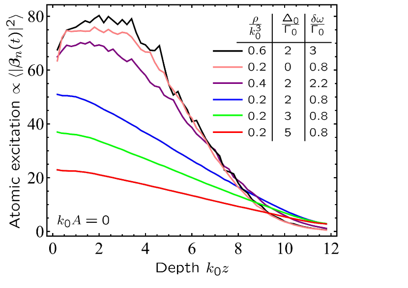
Figure 2: Average profiles of atomic excitation inside a sample of thickness $k_{0}L=12$.

In addition to the dependence of dimensionless conductance on sample thickness, a signature of Anderson localization can be found in the dependence of the average atomic excitation $\langle|\bm{\beta}_{n}(t)|^{2}\rangle$, with the averaging also over time $t$, on the depth $z$ inside the sample [28], see Fig. 2. All curves in Fig. 2 correspond to atomic densities $\rho$ for which Anderson localization is expected at $\delta\omega/\Gamma_{0}=0.8$ for $\Delta_{0}=0$ [24, 25]. We thus expect a step-like (steep in the middle of the sample and flattened towards $z=0$ and $L$) profile of $\langle|\bm{\beta}_{n}(t)|^{2}\rangle$ illustrated by the brown curve in Fig. 2 [28]. However, it is clear that the three lower curves obtained for the same $\rho$ and $\delta\omega$ as the brown curve but in the presence of inhomogeneous broadening $\Delta_{0}\geq 2$, exhibit a roughly linear decay with $z$ characteristic of photon diffusion [28, 23]. Thus, the inhomogeneous broadening suppresses Anderson localization. Nevertheless, similarly to what has been discussed in connection with Fig. 1, this suppression can be mitigated and even fully canceled by increasing $\rho$ and adjusting $\delta\omega$, as clearly witnessed by the violet and black curves in Fig. 2 that exhibit the shape expected for Anderson localization.

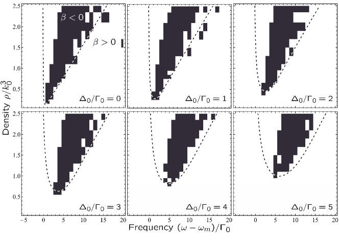
Figure 3: Localization phase diagram for light in a large ensemble of $N\gg 1$ resonant scattering centers embedded in a solid matrix for six different values of inhomogeneous broadening $\Delta_{0}$. $\beta$-function (approximated by a finite difference from numerical results for $N=8$ and $16\times 10^{3}$) is negative and eigenstates are localized in the regions of the phase plane shown in black, whereas $\beta>0$ and states are extended in the rest of the plane. Dashed lines show the mobility edge $\beta=0$ predicted by our approximate analytic theory.

To gain a systematic understanding of the impact of inhomogeneous broadening on Anderson localization, we consider random distributions of $N\gg 1$ atoms in a sphere of diameter $L$ and compute the complex eigenenergies $E_{n}$ of the effective Hamiltonian (1), ordered by their real parts, see Supplementary Information (SI) [46] for details. They define frequencies $\omega_{n}=\omega_{0}-(\Gamma_{0}/2)\text{Re}E_{n}$ and decay rates $\Gamma_{n}=\Gamma_{0}\text{Im}E_{n}$ of quaisimodes of the atomic system. Frequency-dependent Thouless conductance is defined as $g_{\text{Th}}(\omega)=\langle 1/\Gamma_{n}\rangle_{\omega}^{-1}/\langle\omega_{n}-\omega_{n-1}\rangle_{\omega}$ [47, 22] with averaging $\langle\ldots\rangle_{\omega}$ over random realizations of atomic positions $\{{\mathbf{r}}_{n}\}$, frequency shifts $\{\Delta_{n}\}$ and, in addition, eigenenergies $E_{n}$ for which $\omega_{n}$ fall inside a frequency interval of width $\Gamma_{0}$ around $\omega$. To characterize the dependence of $g_{\text{Th}}$ on $L$, we compute $\beta(g_{\text{Th}})=\partial\ln g_{\text{Th}}/\partial\ln(k_{0}L)$. $\beta>0$ in the region of parameters for which quasimodes are extended in space whereas $\beta<0$ for spatially localized eigenmodes [45, 22]. Figure 3 shows localization phase diagrams for light in the large ensemble of resonant scattering centers for different strengths of the inhomogeneous broadening $\Delta_{0}$. For $\Delta_{0}=0$, Anderson localization is expected in a certain range of frequencies only when $\rho/k_{0}^{3}\gtrsim 0.1$ [25]. In agreement with our previous discussion, increasing $\Delta_{0}$ leads to a requirement of higher density to reach localization but does not fully suppress it. An additional illustration of this is provided by Fig. 4 that shows the minimum density at which Anderson localization takes place in our model at any frequency, as a function of $\Delta_{0}$. The minimum density increases with $\Delta_{0}$ but remains finite.

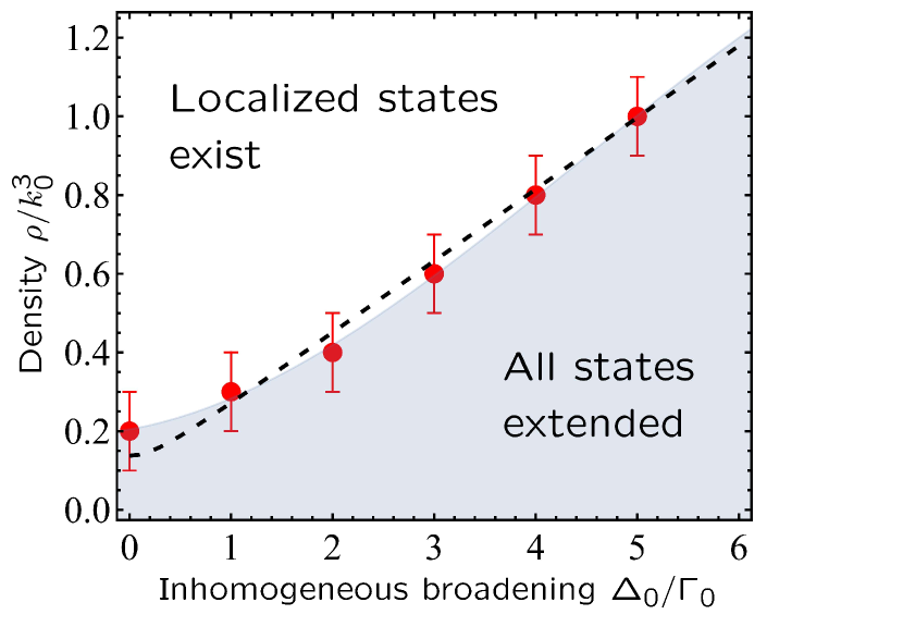
Figure 4: Minimum number density of impurity atoms $\rho$ required for collective atomic states to be spatially localized in some frequency band, as a function of the magnitude of inhomogeneous broadening $\Delta_{0}$ (red disks with error bars). Grey shading shows the region of the parameter space in which all states are extended. Dashed line is the prediction of our approximate analytic theory.

A simple interpretation of results shown in Figs. 3 and 4 can be obtained by averaging the self-energy $\Sigma(\omega)$ obtained in the independent scattering approximation (ISA) [48] over the normal distribution of resonance frequencies $\omega_{nm}$ of individual atoms, see SI [46]. The variance of the distribution is assumed to be equal to a sum of $\Delta_{0}^{2}$ due to the random local electric fields and a term $\sim(\rho/k_{0}^{3})^{2}$ due to dipole-dipole interactions between nearby atoms [46]. This turns out to be a simple yet efficient way of taking into account the two effects otherwise neglected by ISA. We define the effective wave number $k_{\text{eff}}=\text{Re}\sqrt{k_{0}^{2}-\langle\Sigma(\omega)\rangle}$ and the scattering mean free path $\ell=1/2\text{Im}\sqrt{k_{0}^{2}-\langle\Sigma(\omega)\rangle}$. The Ioffe-Regel criterion of localization yields a simple condition for the mobility edge : $k_{\text{eff}}\ell=(k_{\text{eff}}\ell)_{c}\sim 1$ [49, 48, 50]. Dashed lines in Fig. 3 show contour plots of this equation for different $\Delta_{0}$ with $(k_{\text{eff}}\ell)_{c}=0.6$. It captures the main tendency exhibited by the numerical results when $\Delta_{0}$ increases although it is clearly not exact. An even better agreement is obtained for the minimum density required to reach localization in Fig. 4.

In conclusion, we demonstrate that transparent solids with impurity atoms or ions at random positions are promising materials for reaching Anderson localization of light in 3D. On the one hand, the detrimental effect of longitudinal optical fields [22, 23] can be mitigated in these materials by an external magnetic field, in the same way as in cold-atom systems [24, 25], which gives them an advantage over suspensions or powders of dielectric particles [11, 10]. On the other hand, they do not suffer from strong losses characteristic of metallic structures proposed as candidates for observation of Anderson localization of light [18, 12]. The main result of this work is to show that the difficulties specific for solids with impurity atoms—the oscillations of impurity atoms about their equilibrium positions and the inhomogeneous broadening of their spectra due to random local electric fields—are not critical and should not impede observation of Anderson localization of light. Therefore, we believe that it would be worthwhile to put some effort in experimenting with such materials.

I Details of the scaling analysis

We generate independent spatial configurations of $N$ atoms randomly distributed inside a sphere of diameter $L$ at a number density $\rho=N/V$ with $V=\pi L^{3}/6$. For each atom, a random shift $\Delta_{n}$ of its resonance frequency $\omega_{0}$ is sampled from a centered normal distribution with variance $\Delta_{0}^{2}$. For each atomic configuration with a corresponding set of $\Delta_{n}$, complex eigenvalues $E_{n}$ of the effective Hamiltonian (1) are computed numerically and ordered according to their real parts. Then, mean values of $1/\Gamma_{n}$ and of $\omega_{n}-\omega_{n-1}$ are computed in each frequency interval of width $\Gamma_{0}$ from $\delta\omega=\omega-\omega_{m}=-5\Gamma_{0}$ to $20\Gamma_{0}$, where $\omega_{n}=\omega_{0}-(\Gamma_{0}/2)\text{Re}E_{n}$ and $\Gamma_{n}=\Gamma_{0}\text{Im}E_{n}$. Averaging is also performed over a large number of independent atomic configurations in space and over $\{\Delta_{n}\}$. Typically, we average over 50, 35 and 25 configurations for $N=8000$, 12000 and 16000, respectively. Thouless conductance is defined as $g_{\text{Th}}(\omega)=\langle 1/\Gamma_{n}\rangle_{\omega}^{-1}/\langle\omega_{n}-\omega_{n-1}\rangle_{\omega}$, where the notation $\langle\cdots\rangle_{\omega}$ highlights the additional averaging over all $\omega_{n}$ inside an interval of width $\Gamma_{0}$ around the frequency $\omega$.

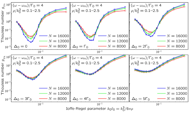
Figure S2: A cut of Fig. S1 at $\delta\omega=\omega-\omega_{m}=4\Gamma_{0}$, intended to demonstrate the transition from Anderson localization for $\Delta_{0}<4$ (curves corresponding to different $N$ cross in points determining mobility edges) to diffuse transport for $\Delta_{0}>4$ (no crossings).

Figure S1 shows $g_{\text{Th}}$ as a function of $k_{0}\ell_{0}=k_{0}^{3}/6\pi\rho$ and $\delta\omega/\Gamma_{0}$, for six different values of $\Delta_{0}$. It is clear that the drop of $g_{\text{Th}}$ around $\delta\omega/\Gamma_{0}=4$ at $\Delta_{0}=0$, shifts to larger $\delta\omega$ and becomes less pronounced with increasing $\Delta_{0}$. The impact of inhomogeneous broadening on Thouless conductance at a given frequency is demonstrated in Fig. S2 for $\delta\omega/\Gamma_{0}=4$. When $\Delta_{0}<4$, localization transitions take place at values of $k_{0}\ell_{0}$ where curves corresponding to different $N$ cross. These transitions are suppressed for $\Delta_{0}>4$, leading to $g_{\text{Th}}$ being a growing function of $N$ at all densities $\rho$. Figure 4 of the main text is obtained by estimating the $\beta$-function $\beta(g_{\text{Th}})=\partial\ln g_{\text{Th}}/\partial\ln(k_{0}L)$ using a finite-difference approximation for the derivative.

II Influence of inhomogeneous broadening on Anderson localization of light in cold atomic clouds: Approximate analytic theory

In the independent scattering approximation, the self-energy is [48, 21]

$$\begin{aligned} \Sigma(\omega,\omega_{0}^{\prime})&=\frac{4\pi\rho}{k_{0}}\times\frac{1}{2(\omega-\omega_{0}^{\prime})/\Gamma_{0}+i}\end{aligned}$$ (S1)

We assume that the atomic resonance frequency $\omega_{0}^{\prime}$ is subject to inhomogeneous broadening due to (i) strong local fields in the transparent host medium and (ii) strong dipole-dipole interactions between nearby atoms. The resulting distribution of $\omega_{0}^{\prime}$ is approximated by a Gaussian:

$$p(\omega_{0}^{\prime}) = \frac{1}{\sqrt{2\pi}\Delta}\exp\left[-\frac{(\omega_{0}^{\prime}-\omega_{0})^{2}}{2\Delta^{2}}\right]$$ (S2)

where $\omega_{0}$ is the resonance frequency in the absence of broadening. The variance of the distribution (S2) is given by a sum of two contributions:

$$\Delta^{2}=\Delta_{0}^{2}+\langle\Delta_{\text{dd}}^{2}\rangle$$ (S3)

First, local fields in the host crystal yield random frequency shifts that we denote by $\Delta_{n}$, with a variance $\Delta_{0}^{2}$. Second, the typical frequency shifts $\Delta_{\text{dd}}$ induced by dipole-dipole interactions are of the order of $1/(k_{0}\Delta r)^{3}\propto\rho/k_{0}^{3}$, where we used the fact that the typical distance between nearby atoms is $\Delta r=\rho^{-1/3}$. To obtain a quantitative estimate, we recall that in a strong magnetic field, the eigenvalues of the Hamiltonian (1) in the main text, yielding eigenfrequencies $\omega$ near resonances $\omega_{m}$ ($m=\pm 1$), can be obtained by diagonalizing a $N\times N$ matrix [24, 25]

$$\begin{aligned} (\hat{H}_{\text{eff}})_{nn^{\prime}}&=\left(i\mp 2\frac{\Delta_{B}}{\Gamma_{0}}\right)\delta_{nn^{\prime}}+(1-\delta_{nn^{\prime}})\frac{3}{2}\frac{e^{ik_{0}\Delta r_{nn^{\prime}}}}{k_{0}\Delta r_{nn^{\prime}}}\\ &\times\left[P(ik_{0}\Delta r_{nn^{\prime}})+Q(ik_{0}\Delta r_{nn^{\prime}})\frac{\sin^{2}\theta_{nn^{\prime}}}{2}\right]\end{aligned}$$ (S4)

where $\theta_{nn^{\prime}}$ is the angle between the vector $\Delta{\mathbf{r}}_{nn^{\prime}}={\mathbf{r}}_{n}-{\mathbf{r}}_{n^{\prime}}$ and the quantization axis $z$. To be specific, let us consider $m=1$. For two atoms ($N=2$) at a distance $\Delta{\mathbf{r}}={\mathbf{r}}_{2}-{\mathbf{r}}_{1}$ the two eigenvalues of the matrix (S4) are

$$\begin{aligned} E_{\pm}&=\left(i-2\frac{\Delta_{B}}{\Gamma_{0}}\right)\pm\frac{3}{2}\frac{e^{ik_{0}\Delta r}}{k_{0}\Delta r}\\ &\times\left[P(ik_{0}\Delta r)+Q(ik_{0}\Delta r)\frac{\sin^{2}\theta}{2}\right]\end{aligned}$$ (S5)

and frequency shifts with respect to $\omega_{1}=\omega_{0}+\Delta_{B}$ are $(\Delta_{\text{dd}})_{\pm}=-(\Gamma_{0}/2)\text{Re}E_{\pm}-\Delta_{B}$. Averaging over the two eigenvalues and over $\theta$ yields

$$\langle\Delta_{\text{dd}}\rangle = 0$$ (S6)

$$\begin{aligned} &\langle\Delta_{\text{dd}}^{2}\rangle=\frac{3}{160}\left(\frac{\rho}{k_{0}^{3}}\right)^{\frac{2}{3}}\left\{3\left(\frac{\rho}{k_{0}^{3}}\right)^{\frac{4}{3}}+\left(\frac{\rho}{k_{0}^{3}}\right)^{\frac{2}{3}}\right.\\ &\left.+\left[3\left(\frac{\rho}{k_{0}^{3}}\right)^{\frac{4}{3}}-5\left(\frac{\rho}{k_{0}^{3}}\right)^{\frac{2}{3}}+7\right]\cos\left[2\left(\frac{\rho}{k_{0}^{3}}\right)^{-\frac{1}{3}}\right]\right.\\ &+\left.\left[6\left(\frac{\rho}{k_{0}^{3}}\right)-2\left(\frac{\rho}{k_{0}^{3}}\right)^{\frac{1}{3}}\right]\sin\left[2\left(\frac{\rho}{k_{0}^{3}}\right)^{-\frac{1}{3}}\right]+7\right\}\\ &\to\frac{9}{80}\left(\frac{\rho}{k_{0}^{3}}\right)^{2}\end{aligned}$$ (S7)

where in the last line we have taken the limit $\rho/k_{0}^{3}\gg 1$.

The average self-energy is

$$\langle\Sigma(\omega,\omega_{0})\rangle = \int\limits_{-\infty}^{\infty}d\omega_{0}^{\prime}p(\omega_{0}^{\prime})\Sigma(\omega,\omega_{0}^{\prime})$$ (S8)

The effective complex wave number is

$$\sqrt{k_{0}^{2}-\langle\Sigma(\omega,\omega_{0})\rangle} = k+\frac{i}{2\ell}$$ (S9)

and hence

$$k = \text{Re}\sqrt{k_{0}^{2}-\langle\Sigma(\omega,\omega_{0})\rangle}$$ (S10)

$$\ell = \frac{1}{2\;\text{Im}\sqrt{k_{0}^{2}-\langle\Sigma(\omega,\omega_{0})\rangle}}$$ (S11)

Ioffe-Regel criterion of localization is

$$k\ell = \frac{\text{Re}\sqrt{k_{0}^{2}-\langle\Sigma(\omega,\omega_{0})\rangle}}{2\;\text{Im}\sqrt{k_{0}^{2}-\langle\Sigma(\omega,\omega_{0})\rangle}}=(k\ell)_{c}\sim 1$$ (S12)

Comparison of contour plots of this equation with the localization phase diagram following from numerical calculations is shown in Fig. 3 of the main text.

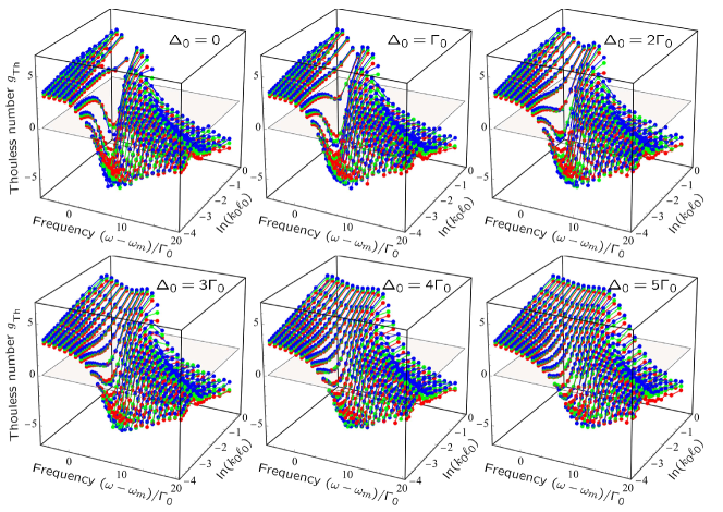
Figure S1: Thouless conductance $g_{\text{Th}}$ as a function of the bare Ioffe-Regel parameter $k_{0}\ell_{0}=k_{0}^{3}/6\pi\rho$ and frequency detuning $\delta\omega=\omega-\omega_{m}$, for six different values of inhomogeneous broadening $\Delta_{0}$. Data obtained for different total numbers of atoms are shown in different colors: $N=8000$ (red), 12000 (green), 16000 (blue). The explored range of $k_{0}\ell_{0}$ corresponds to the range $\rho/k_{0}^{3}=0.1$–2.5 of the atomic number density.