Resampling and averaging coordinates on data

Abstract.

We introduce algorithms for robustly computing intrinsic coordinates on point clouds. Our approach relies on generating many candidate coordinates by subsampling the data and varying hyperparameters of the embedding algorithm (e.g., manifold learning). We then identify a subset of representative embeddings by clustering the collection of candidate coordinates and using shape descriptors from topological data analysis. The final output is the embedding obtained as an average of the representative embeddings using generalized Procrustes analysis. We validate our algorithm on both synthetic data and experimental measurements from genomics, demonstrating robustness to noise and outliers.

1. Introduction

A central postulate of modern data analysis is that the high-dimensional data we measure in fact arises as samples from a low-dimensional geometric object. This hypothesis is the basic justification for dimensionality reduction which is the first step in almost all geometric data analysis algorithms, particularly in clustering and its higher dimensional analogs. This is aimed at mitigating the “curse of dimensionality”, a broad term for various concentration of measure results that imply that the geometry of high-dimensional Euclidean spaces behaves very counter-intuitively. The curse of dimensionality tells us that if this hypothesis is not satisfied, we cannot expect to perform any meaningful inference at all.

The recent explosion of data acquisition processes in many different scientific fields (e.g., single-cell RNA sequencing experiments in computational biology, realistic synthetic data sets obtained from deep generative models, multivariate time series generated from large numbers of sensors, etc.) has led to a dramatic increase of publicly available data sets in high ambient dimensions. The need for tractable and accurate data science tools for processing these data sets has thus become critical. While supervised machine learning and deep learning methods have proven to be very efficient in many different areas and applications of data science, they are often limited by the difficulty of finding suitable training data. Hence, the problem of studying this data via dimensionality reduction and exploratory data analysis has become central.

However, dimensionality reduction algorithms generally have the inherent complication that they depend on a variety of ad hoc hyperparameters and are sensitive both to noise concentrated around the underlying geometric object and to outliers. Moreover, all methods are known to be very sensitive to these hyperparameters: a slight change in only one parameter can lead to dramatic changes in the output lower-dimensional embeddings. As a consequence, it is challenging to perform meaningful inference based on such procedures and most serious applications involve a lot of ad hoc cross-validation procedures.

This article proposes a method to resolve this issue by producing robust embeddings, employing the following process:

• Subsampling and varying hyperparameters to produce a number of embeddings of a given (low) dimension using dimensionality reduction techniques,

• using affine isometries and the solution to the general “Procrustes problem” to align the embeddings in a way that minimizes a certain natural metric (explained below),

• clustering the aligned embeddings based on that metric,

• identifying a cluster of “representative” embeddings by looking at the cluster density and using topological data analysis (TDA) to eliminate clusters with topologically complex embeddings, and

• taking the average (centroid) of the embeddings in the representative cluster to produce a final low dimensional embedding of most of the points. (Points which are not present in the averaged embeddings are returned as “outliers”.)

The subsampling leads to results that are robust with respect to isotropic noise and have reduced sensitivity to outlier data points. The clustering discards outlier embeddings with a high level of distortion. Essentially any dimensionality reduction algorithm can be used, but the procedure works best when the algorithm preserves some global structure; e.g., t-SNE and UMAP, which preserve local relationships but can radically distort global relationships produce less sharp results. (See Section 8 for further discussion of this point.) The intuition behind our use of TDA invariants (notably persistent homology) to detect the representative embeddings is that we expect coordinate charts to be contractible subsets: theoretical guarantees for manifold learning imply that the algorithms really only work in this case. Persistent homology is a convenient way to detect complicated topological features such as holes.

We illustrate the process in Figure 1. The figure shows a standard 3-dimensional “Swiss roll” synthetic data set and uses Isomap to produce a $2$-dimensional coordinate chart. This is a particularly easy example, but we achieve similar results in the presence even of a large number of outliers and across parameter regimes. See Section 7 for a variety of synthetic examples.

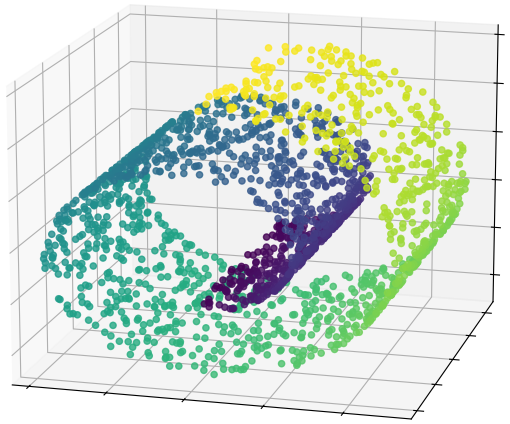
(a) Original data in 3D

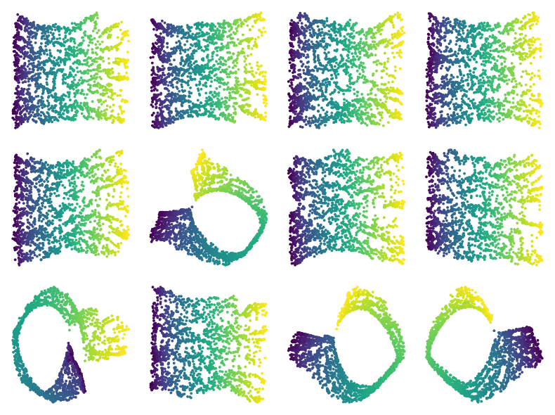
(b) Isomap results on subsamples

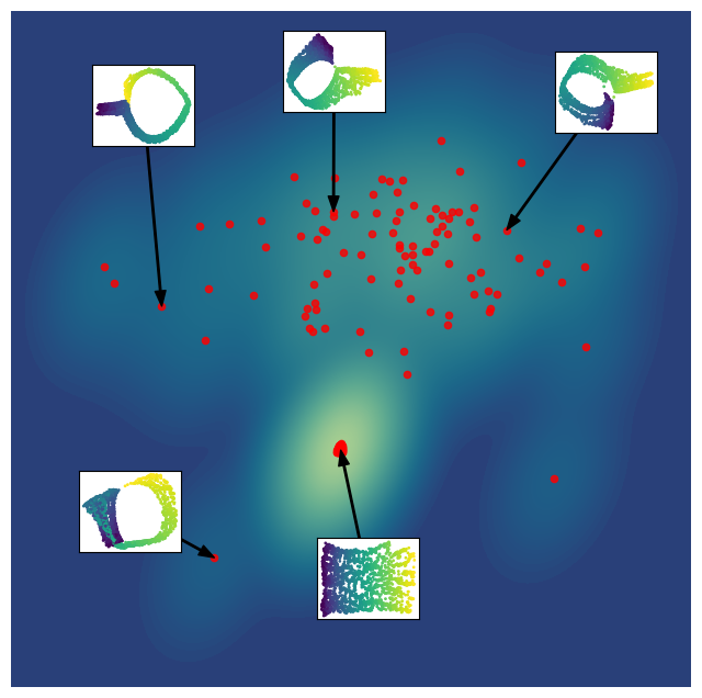
(c) Clustering embeddings

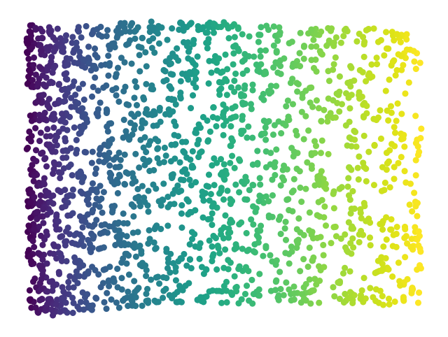
(d) Final aligned output

Figure 1. Swiss roll dataset

The discussion above emphasizes the robustness in the presence of outliers, but our technique has an additional use case where it can be employed to reduce the computational complexity of dimensionality reduction computations: instead of computing a dimensionality reduction of the entire data set, the procedure above can be used to produce a global set of coordinates by averaging coordinates from much smaller subsamples.

In order to demonstrate the use of our procedure on real data, we apply it to multiple dimensionality reduction methods for producing coordinates on genomic data sets in Section 8, specifically blood cells (PBMC) and mouse neural tissue. The results show that our procedure can be used to produce robust coordinates from some manifold learning algorithms and indicates the instability of coordinates produced from others.

Related work

Procrustes analysis has long been used to study shapes [17]. Building on scaling methods, the orthogonal Procrustes problem was first studied and solved by Green [16], and Schönemann and Schönemann-Carroll [25, 26], and later this was generalized to three or more shapes by Gower [14]. Nowadays, there are many variants of Procrustes problems. Beyond statistical shape analysis [13], Procrustes analysis has found applications in sensory science [11], market research [15], image analysis [12], morphometrics [8], protein structure [22], environmental science [24], population genetics [34], phylogenetics [4], chemistry [1], ecology [20], and more. In forthcoming work, the authors will present an application to neuroscience.

The early applications of Procrustes analysis were in the field of psychometrics, where point sets are registered to a single “reference” profile that is sometimes realized in physical space, and datasets are small. More recently, it has been increasingly recognized that the same techniques and ideas can be applied just as well to the shape of “data” itself with no expectation of a reference whatsoever, and to high-dimensional datasets [2] with many samples. For example, [21] uses a version of Procrustes analysis with shuffling to align low-rank representations of single cell transcriptomic data. Procrustes analysis can also be applied to statistics itself. In this sense, part of our current study can be viewed as an expansion of [19], which studied a jackknife procedure on multidimensional scaling, a limited form of manifold learning. Similarly, [33] applied Procrustes analysis to the outputs of dimensionality reduction, specifically Laplacian eigenmaps and locality preserving projections, but only for two point clouds at a time.

Summary

In Section 2, we provide a concise review of the background for our work; we discuss manifold learning and dimensionality reduction algorithms, the Procrustes distance and alignment problem, and topological data analysis. Next, in Section 3, we describe our algorithm. We then begin a theoretical analysis of the behavior of our algorithm by reviewing in detail the solution to the generalized Procrustes problem in Section 4. We employ a solver based on alternating least squares minimization, and we describe the stability and convergence behavior of this process in Section 5. We then use this to analyze the stability of our algorithm in Section 6. The paper concludes with two sections exploring the behavior of our algorithm: Section 7 studies how it works on simulated data with various kinds of noise and outliers, and Section 8 applies our algorithm to single-cell RNAseq data.

Code availability

For aligning two point clouds, we used the command scipy.spatial.procrustes from the SciPy library [32]. For general Procrustes alignment of two or more point clouds, we developed our own software implementation based on alternating minimization, which can be found at github.com/jhfung/Procrustes.

Acknowledgments

We thank Abby Hickok and Raul Rabadan for useful comments.

2. Background about manifold learning, topological data analysis, and Procrustes distance

Our algorithm uses as building blocks three fundamental concepts from geometric data analysis. The first building block is dimensionality reduction. Our algorithm takes as a black box a choice of dimensionality reduction algorithm. We use manifold learning for this purpose, and to be concrete, we will focus on Isomap, but many other manifold learning (or more general dimensionality reduction algorithms) could be used instead. Manifold learning seeks to find intrinsic coordinates on data that reflects the shape of the data. The second building block is persistent homology, which is the main invariant of topological data analysis (TDA). Persistent homology is a multiscale shape descriptor that provides qualitative shape information; we will use it to detect when coordinate charts are spread out and have contractible components. The third building block is the Procrustes distance, which is a matching distance for (partially defined) vector-valued functions on a given finite set. Computing the Procrustes distance involves computing an optimal alignment of the vectors; our algorithm uses both the distance as a metric and also the computation of the distance as an alignment algorithm.

The manifold learning algorithm takes a point cloud $X\subset\mathbb{R}^{N}$ and produces an embedding $X\to\mathbb{R}^{d}$ for $d\ll N$ meant to retain the intrinsic relationship between the points of $X$. Specifically, for Isomap, the procedure is as follows. Given a point cloud $X\subset\mathbb{R}^{N}$ and a scale parameter $\epsilon>0$ (or a nearest neighbor limit $\ell$), we form the weighted graph $G$ with vertex set labelled by the points $X$ and an edge of weight $\lVert x-x^{\prime}\rVert$ when $\lVert x-x^{\prime}\rVert<\epsilon$ (or when $x^{\prime}$ is one of the $\ell$ closest points to $x$). The graph metric on $G$ now provides a new metric on the point cloud $X$. Finally, we use MDS (multidimensional scaling) to embed this new metric space into $\mathbb{R}^{d}$, for $d\ll N$. The intuition is that when the data $X$ comes from a low dimensional manifold embedded in a high dimensional space, short paths in the ambient space accurately reflect an intrinsic notion of nearness in the manifold. When the points $X$ have been uniformly sampled from a convex subset of a manifold such that $\epsilon$ is sufficiently small relative to the curvature of the manifold and the injectivity radius of the embedding (which can be described in terms of the reach or condition number of the manifold), the coordinates produced by this procedure do approximate the intrinsic Riemannian metric on $X$.

Topological data analysis uses invariants from algebraic topology that encode qualitative shape information to give a picture of the intrinsic geometry of a point cloud. The $q$th homology of a topological space $T$ is a vector space which encodes the $q$-dimensional holes in $T$; for example, when $q=0$ this is measuring the number of path-connected components of the space and when $q=1$ it is counting the number of circles that are not filled in. Topological data analysis assigns to a point cloud a family of associated simplicial complexes, usually filtered by a varying feature scale parameter. The resulting algebraic invariant, persistent homology, captures the scales at which homological features appear and disappear. In the case when $q=0$, the persistent homology is basically the single-linkage hierarchical clustering dendrogram. When $q=1$, persistent homology measures the number of loops in the underlying graph of the data that cannot be filled in at each scale.

Since manifold learning only really makes sense for relatively evenly sampled points from subsets whose components are contractible (or in the case of Isomap, the stronger condition of being convex), we can use topological data analysis to measure how well the resulting chart appears to satisfy this condition. Specifically, a good chart will have a large cluster for each component in the $PH_{0}$ dendrogram and will have only very small (noise) loops in $PH_{1}$.

The Procrustes distance we use comes from the Procrustes problem. In basic form, given two $d\times n$ matrices $X$ and $Y$, thought of as two functions from $\{1,\dotsc,n\}$ to $\mathbb{R}^{d}$, the Procrustes distance is the minimum of the $\ell^{2}$ distances between the functions after applying an affine isometry $g$ to one of them:

$$\mathcal{D}(X,Y)=\min_{g}d(g\cdot X,Y)=\min_{g}\left({\sum_{j=1}^{n}d(g\cdot X(j),Y(j))^{2}}\right)\raisebox{5.38193pt}{\mbox{${}^{1/2}$}}.$$

More generally, we consider the case when $X$ and $Y$ are partially defined functions on $\{1,\dotsc,n\}$. If we let $I_{X}$ and $I_{Y}$ denote the subsets of $\{1,\dotsc,n\}$ where $X$ and $Y$ (respectively) are defined, then the Procrustes distance is

$$\mathcal{D}(X,Y)=\min_{g}\left({\sum_{j\in I_{X}\cap I_{Y}}d(g\cdot X(j),Y(j))^{2}}\right)\raisebox{5.38193pt}{\mbox{${}^{1/2}$}}.$$

The algorithm for calculating $\mathcal{D}$ finds an affine isometry $g$ minimizing the distance; we review it in Section 4. We note that in the partially defined case, the resulting Procrustes distance $\mathcal{D}$ is not a metric; however, for functions with substantial overlap in domain, it does provide a measure of dissimilarity on their overlap.

Our algorithm uses a generalization of the Procrustes distance algorithm to search for optimal rotations to align different embeddings. The algorithm for two matrices always finds an optimal rotation (and therefore accurately calculates the Procrustes distance) and in principle gives an exact solution. The algorithm to align more than two matrices is an iterative optimization procedure, which always converges, and appears to generically converge to the optimal solution, but is not guaranteed to converge to it.

3. The algorithm

This section defines the basic algorithm we propose in this paper. It admits several choices of blackbox subroutines and tolerance parameters. The first major blackbox subroutine is a procedure DimRed for dimensionality reduction: for $X\subset\mathbb{R}^{N}$ produces an embedding $X\to\mathbb{R}^{d}$ (where $d\ll N$). We let $\Theta$ denote the collection of parameters controlling the behavior of the dimensionality reduction procedure. For sake of discussion, we take the procedure to be Isomap, which has parameter the neighborhood size $\epsilon$.

A second major blackbox subroutine is a sampling procedure Samp that generates random subsamples $Y\subseteq X$ of a given size $n$. Typically, we draw $Y_{i}$ uniformly and independently without replacement from $X$.

A third major blackbox subroutine is a procedure Param that chooses the parameter $\Theta$ for DimRed. In the case of Isomap, typically we take the parameter over a mesh of reasonable values.

The final major blackbox subroutine is a clustering algorithm Clust for finite sets with dissimilarity measures.

We describe the various minor parameters controlling the number of iterations, tolerances for certain optimization procedures, number of subsamples, etc., as they occur below.

Given the parameter choices, the input to the algorithm is a point cloud

$$X=\{X(j)\mid j=1,\dotsc,n\}\subset\mathbb{R}^{N}.$$

Step 1

We use Samp to generate many subsamples $\{Y_{a}\}$ and apply DimRed with parameter settings from Param to produce embeddings $\phi_{a,b}\colon Y_{a}\to\mathbb{R}^{d}$. Let $X_{a,b}$ be the subset of $\mathbb{R}^{d}$ specified by the image, where the elements of each subsample configuration $X_{a,b}$ inherit the indexing of original data set $X$. That is, each $X_{a,b}$ is indexed by the subset of $\{1,\dotsc,n\}$ corresponding to the points of $X$ represented in the subsample $Y_{a}$.

Step 2

We calculate the pairwise distances between the images $X_{a,b}$ using the Procrustes distance to define a dissimilarity measure on the set of subsample configurations $\{X_{a,b}\}$ a pseudo-metric space.

Step 3

We use Clust to form clusters.

Step 4

Choose a distinguished cluster (the “good cluster”) from among these as follows.

• We discard clusters whose median inter-point distance is above a certain tolerance (a minor parameter of the algorithm). We refer to the remaining clusters as “dense clusters”.
  

• For each dense cluster we select random elements in the cluster (the number or percentage size of the selection a minor parameter of the algorithm) on which to calculate the persistent homology $PH_{1}$ and essential dimensionality (number of singular values above given tolerance).
  

• We discard dense clusters where a selected element has essential dimensionality less than $d$, and then we choose the good cluster to be the one that minimizes the maximum length of bars in $PH_{1}$.
  

• If there are no remaining clusters or the maximum length of bars in $PH_{1}$ is above a certain tolerance (a minor parameter of the algorithm), we terminate with an error.

Step 5

We discard all the subsets $X_{a,b}$ not in the good cluster, and singularly reindex the subsets in the good cluster $X_{i}=X_{a_{i},b_{i}}$ for $i=1,\dotsc,k$ (with $k$ the number of $X_{a,b}$ in the good cluster).

Step 6

We align the embeddings $X_{i}$ by applying an affine isometry $X_{i}(j)\mapsto Q_{i}X_{i}(j)+v_{i}$ to each point $X_{i}(j)$ in $X_{i}$ (for the indices $j\in\{1,\dotsc,n\}$ that occur in $X_{i}$) where $Q_{i}$ is a $d\times d$ orthogonal matrix and $v_{i}$ is a vector in $\mathbb{R}^{d}$, chosen by the alternating least squares method described in Section 4.

Output

The final output is an appropriate average of the aligned embeddings as follows. For each point $X(j)$ in $X$ ($j=1,\dotsc,n$):

• If no $X_{i}$ includes a $j$th point, then the $j$th point is omitted from the final embedding; otherwise,

• The final embedding has $j$th point the average in $\mathbb{R}^{d}$ of the $j$th points of the $X_{i}$ which have $j$th points,

  $$\bar{X}(j)=\tfrac{1}{s}(X_{i_{1}}(j)+\dotsb+X_{i_{s}}(j)).$$

• We also output a list of “outliers” that consists of the omitted indices, the indices that did not have points in any of the embeddings $X_{i}$ chosen to produce the final average.

4. A review of the Procrustes problem

Our main ingredient for averaging coordinates is posing the averaging in terms of the so-called Procrustes problem, an alignment problem that has been studied extensively in the psychometrics literature. The material in this section distills the discussion in [5, 9, 6].

The standard orthogonal and affine orthogonal Procrustes problem

In its most standard form, given two matrices $X,Y$ of the same shape, this problem is a matrix approximation problem that aims at finding the best orthogonal matrix that matches $X$ to $Y$:

(4.1) $$Q_{\min}=\underset{Q\ {\rm s.t.}\ Q^{T}Q=1}{{\rm argmin}}\|QX-Y\|_{F},$$

where $\|\cdot\|_{F}$ denotes the Frobenius norm (the square root of the sum of the squares of the entries). By interpreting $Q_{\min}$ as an isometry (in Euclidean space), and $X,Y$ as point clouds (each column representing a point), the standard Procrustes problem can thus be seen as an alignment problem which aims at finding the best orthogonal transformation that transports the point cloud $X$ closest to the point cloud $Y$ in terms of the sum of pointwise distances. In practice, it can reformulated as finding the best orthogonal matrix $Q_{\min}$ approximating the given matrix $YX^{T}$, and proved to be efficiently solved by computing the SVD of

$$YX^{T}=U\Sigma V^{T}$$

(with $U$ and $V$ orthogonal and $\Sigma$ non-negative diagonal) and taking $Q_{\min}=UV^{T}$.

If we allow the more general affine isometries (that allow a translation component), it is easy to check that

(4.2) $$\Omega_{\min}=\underset{\Omega\in\mathcal{A}f\!f(d)}{{\rm argmin}}\|\Omega X-Y\|_{F},$$

is given by the affine isometry

$$\Omega_{\min}x=Q(x-a)+b=Qx+(b-Qa)$$

where $a$ is the centroid (mean) of $X$, $b$ is the centroid of $Y$, and $Q$ is the orthogonal matrix $Q_{\min}$ that solves equation (4.1) for the matrices $X-\mathbf{1}a$ and $Y-\mathbf{1}b$ (where $\mathbf{1}$ is the $1\times n$ matrix of $1$s: the matrices $X-\mathbf{1}a$ and $Y-\mathbf{1}b$ are the translations of $X$ and $Y$ to be centered on the origin.)

In the notation of Section 2, the Procrustes distance $\mathcal{D}(X,Y)$ from $X$ to $Y$ is then

$$\mathcal{D}(X,Y)=\lVert\Omega_{\min}X-Y\rVert_{F}.$$

As discussed in Section 2, we need to consider the more general case when the matrices are missing columns; we refer to this as the missing points case. Viewing $d\times n$ matrices as functions $\{1,\dotsc,n\}$ to $\mathbb{R}^{d}$, the missing points case is when we have partially defined functions $X$ and $Y$ from $\{1,\dotsc,n\}$ to $\mathbb{R}^{d}$; that is $X$ and $Y$ are functions from subsets $I_{X}$ and $I_{Y}$ of $\{1,\dotsc,n\}$ to $\mathbb{R}^{d}$. Let $I$ be the natural reindexing of the intersection of the domains $I_{X}\cap I_{Y}$. Then the Procrustes distance $\mathcal{D}(X,Y)$ as defined in Section 2 is calculated by the formula

$$\mathcal{D}(X,Y)=\lVert\Omega_{\min}X_{I}-Y_{I}\rVert_{F}$$

where $\Omega_{\min}$ solves (4.2) for the matrices $X_{I}$, $Y_{I}$ (the matrices obtained by restricting $X$ and $Y$ to $I_{X}\cap I_{Y}$).

Background on the generalized Procrustes problem

The formulation of the Procrustes problem in the previous subsection involved only 2 matrices or matrices missing points (partially defined functions). In this subsection, we begin the discussion of the problem for multiple matrices. We then generalize to the missing points case and discuss algorithms in the following subsections.

We begin with some notation. Let $X_{1},X_{2},\ldots,X_{k}$ be a collection of $k$ point clouds, each containing $n$ ordered points in $\mathbb{R}^{d}$. We can represent each $X_{i}$ as a $d\times n$ matrix, and denote the collection of such by $\mathbf{X}=(X_{i})$. The allowable transformations will be drawn from a group $G$, which we generally take to be the group of linear isometries (orthogonal transformations) or affine isometries of $\mathbb{R}^{d}$. We write $g_{i}\in G$ for the transformation that will be applied to the $i$th point cloud $X_{i}$, and $\mathbf{g}=(g_{i})$ for the collection of them.

Definition 4.3.

The generalized Procrustes problem is the following: given $\mathbf{X}$, a set of $k$ input configurations of $n$ points in $\mathbb{R}^{d}$ and group $G$ acting continuously on $\mathbb{R}^{d}$, determine the optimal transformations $\mathbf{g}$ and configuration $Z$ that minimizes the loss functional

$$\mathcal{E}(\mathbf{X},\mathbf{g},Z)=\frac{1}{k}\sum_{i=1}^{k}\lVert g_{i}\cdot X_{i}-Z\rVert^{2}_{F}=\frac{1}{k}\sum_{i=1}^{k}\sum_{j=1}^{n}\lVert g_{i}\cdot X_{i}(j)-Z(j)\rVert^{2}$$

The existence of solutions to Procrustes problems in the groups we are interested in follows from simple considerations.

Proposition 4.4.

If $G$ is compact or the semi-direct product of a compact group and the translation group, then $\mathcal{E}$ achieves a global minimum.

The solution is never unique when $G$ contains non-identity isometries of $\mathbb{R}^{d}$ because for any $\mathbf{X},\mathbf{g},Z$, and any isometry $h\in G$, writing $h\mathbf{g}$ for $(hg_{i})$, we have

$$\mathcal{E}(\mathbf{X},\mathbf{g},Z)=\mathcal{E}(\mathbf{X},h\mathbf{g},h\cdot Z).$$

In the case when $G$ a subgroup of the isometries of $\mathbb{R}^{d}$, we can eliminate this trivial duplication of solutions by considering only solutions that have $g_{1}$ a fixed element of $G$, possibly depending on $\mathbf{X}$. An obvious choice is to take $g_{1}$ to be the identity, but the choice we take below is to choose $g_{1}$ to be the translation that centers $X_{1}$ on $0\in\mathbb{R}^{d}$. The first fixed formulation of the generalized Procrustes problem (for $G$ the group of affine isometries) is to find $\mathbf{g},Z$ minimizing the loss functional and satisfying the further condition that $g_{1}$ is the translation that centers $X_{1}$ on $0\in\mathbb{R}^{d}$.

We now specialize to the case where $G$ is the group of affine isometries $\mathcal{A}f\!f(d)$ (consisting of composites of translations, rotations, and reflections in $\mathbb{R}^{d}$). We specify an element $g$ of $G$ by a $d\times d$ orthogonal matrix $Q$ and a vector $v$, where for $x\in\mathbb{R}^{d}$,

$$g\cdot x=Qx+v.$$

On a configuration $X$, viewed as a $d\times n$ matrix, the action is given by matrix multiplication and addition

$$g\cdot X=QX+\mathbf{1}v$$

where $\mathbf{1}$ denotes the $1\times n$ matrix of $1$s.

A key observation is that we can eliminate translations and $Z$ as variables in the generalized Procrustes problem:

Proposition 4.5.

For fixed $\mathbf{X}$, the minimum value of $\mathcal{E}(\mathbf{X},\mathbf{g},Z)$ occurs at elements $\mathbf{g}$, $Z$ where the centroid of each $g_{i}X_{i}$ is the origin and each $Z(j)$ is the average of $X_{i}(j)$,

$$Z(j)=\frac{1}{k}\sum_{i=1}^{k}g_{i}\cdot X_{i}(j).$$

Proof.

We begin with the translation part. For fixed $\mathbf{X},\mathbf{g}$, $Z$, let $q\in 1,\dotsc,k$, let $v\in\mathbb{R}^{d}$, and consider the path $\mathbf{g}(t)$ in $G^{k}$ where $g_{i}(t)=g_{i}$ for $i\neq q$, and $g_{q}(t)$ is the composite of $g_{q}$ followed by the translation $x\mapsto x+tv$. Then

$$\left.\frac{d}{dt}\right|_{t=0}\mathcal{E}(\mathbf{X},\mathbf{g}(t),Z) =\frac{2}{k}\sum_{i=1}^{k}\sum_{j=1}^{n}\left((g_{i}\cdot X_{i}(j)-Z(j))\cdot\left.\frac{d}{dt}\right|_{t=0}(g_{i}(t)\cdot X_{i}(j)-Z(j))\right)$$

$$=\frac{2}{k}\sum_{j=1}^{n}(g_{q}\cdot X_{q}(j)-Z(j))\cdot v.$$

If $\mathbf{g},Z$ gives a minimum for $\mathcal{E}(\mathbf{X},\mathbf{g},Z)$ then this derivative must be zero for every $q$ and $v$, which implies that

$$\sum_{j=1}^{n}Z(j)=\sum_{j=1}^{n}g_{q}\cdot X_{q}(j)$$

for all $q$, and so all the $g_{i}\cdot X_{i}$ and $Z$ must have the same centroid. Thus, the minimum can only occur for a $g_{i}$ that centers $X_{i}$ on the centroid of $Z$. In the first fixed formulation, the common centroid of $Z$ and the $X_{i}$ is then the origin. More generally, taking advantage of the symmetry of the problem as a whole, given a solution $\mathbf{g},Z$, there exists a solution with the common centroid at the origin by applying an appropriate translation.

To eliminate $Z$ as a variable, if we keep $\mathbf{g}$ fixed and for some $r\in 1,\dotsc,n$, let $Z_{t}$ be the path with $Z_{t}(j)=Z(j)$ for $j\neq r$ and $Z_{t}(r)=Z(j)+tv$, we then have

$$\left.\frac{d}{dt}\right|_{t=0}\mathcal{E}(\mathbf{X},\mathbf{g},Z_{t}) =\frac{2}{k}\sum_{i=1}^{k}\sum_{j=1}^{n}\left((g_{i}\cdot X_{i}(j)-Z(j))\cdot\left.\frac{d}{dt}\right|_{t=0}(g_{i}\cdot X_{i}(j)-Z_{t}(j))\right)$$

$$=\frac{2}{k}\sum_{i=1}^{k}(g_{i}\cdot X_{i}(r)-Z(r))\cdot v.$$

In the case when $\mathbf{g},Z$ gives a minimum for the loss functional, we then conclude

$$Z(r)=\frac{1}{k}\sum_{i=1}^{k}g_{i}\cdot X_{i}(r)$$

for all $r$. The minimum can only occur when $Z(j)$ is the average over $i$ of the $g_{i}\cdot X_{i}(j)$. ∎

By Proposition 4.5, we do not need to search over the space of $Z$ and we can restrict to searching for the orthogonal transformation part of the $g_{i}$. This leads to the centered formulation of the problem.

Definition 4.6.

The centered formulation of the generalized Procrustes problem for the group of affine isometries is the following: given $\mathbf{X}$, a set of $k$ input configurations of $n$ points in $\mathbb{R}^{d}$ whose centroids are the origin, determine the optimal orthogonal transformations $\mathbf{Q}=(Q_{i})\in O(d)^{n}$ that minimize the loss functional

$$\mathcal{E}(\mathbf{X},\mathbf{Q})=\frac{1}{k}\sum_{i=1}^{k}\lVert Q_{i}X_{i}-Z\rVert^{2}_{F}=\frac{1}{k}\sum_{i=1}^{k}\sum_{j=1}^{n}\lVert Q_{i}X_{i}(j)-Z(j)\rVert^{2}$$

where $Z(j)=\frac{1}{k}\sum Q_{i}X_{i}(j)$.

There is always a solution with $Q_{1}=\mathrm{Id}$; the centered first fixed formulation is to find the optimal $\mathbf{Q}$ subject to the restriction that $Q_{1}=\mathrm{Id}$.

In the centered formulation, because $Z$ is the mean of the $Q_{i}X_{i}$, we can rewrite the loss functional in the following form, which is sometimes more convenient:

(4.7) $$\mathcal{E}(\mathbf{X},\mathbf{Q})=\frac{1}{k}\sum_{i=1}^{k}\bigl{(}\lVert Q_{i}X_{i}\rVert^{2}_{F}-\lVert Z\rVert^{2}_{F}\bigr{)}.$$

Expanding out the definition of $Z$, this is then:

(4.8) $$\mathcal{E}(\mathbf{X},\mathbf{Q})=\frac{1}{k}\sum_{i=1}^{k}\biggl{(}\lVert Q_{i}X_{i}\rVert^{2}_{F}-\lVert\frac{1}{k}\sum_{i=1}^{k}Q_{i}X_{i}\rVert^{2}_{F}\biggr{)}.$$

The alternating least squares (ALS) method for the generalized Procrustes problem

The background in the previous subsection suggests the following algorithm for searching for the solution to the generalized Procrustes problem for the group of affine isometries. In the centered formulation, we iteratively use the 2 matrix Procrustes problem solution applied to $X_{i}$ and $Z$, to get better and better matches between each $Q_{i}X_{i}$ and the mean of the $Q_{i}X_{i}$. For the non-centered formulation, we first reduce to the centered formulation by translating the original configurations to be centered on the origin.

We state the algorithm in the centered formulation, where we are given the input configurations $\mathbf{X}$, where we assume each $X_{i}$ is centered on the origin, and we search for the orthogonal matrices $\mathbf{Q}$ minimizing the loss functional $\mathcal{E}$ of Definition 4.6. We assume a small number $\rm{tol}$ as a pre-selected tolerance for termination and a large integer $\rm{max\_iter}$ for a maximum number of iterations.

Algorithm (Basic ALS method).

1. Initialize $Z=\frac{1}{k}\sum_{i=1}^{k}X_{i}$.

2. Set $\mathrm{loss}=\mathcal{E}(\mathbf{X},\mathbf{Q})$.

3. Use SVD to solve $ZX_{i}^{T}=U_{i}\Sigma_{i}V_{i}^{T}$ (for $i=1,\dotsc,k$) where $U_{i}$, $V_{i}$ are orthogonal $d\times d$ matrices and $\Sigma_{i}$ is a non-negative diagonal matrix with diagonal entries in decreasing order.

4. Update $Z=\frac{1}{k}\sum_{i=1}^{k}U_{i}V_{i}^{T}X_{i}$.

5. If $|\mathrm{loss}-\mathcal{E}(\mathbf{X},\mathbf{Q})|\geq\mathrm{tol}$ and the number of iterations is less than $\rm{max\_iter}$, iterate from Step 1. Else:

6. Return $(U_{i}V_{i}^{T}),Z$.

We have written the algorithm to emphasize the concept; it admits many tweeks to increase efficiency, some of which are discussed after the final version of the algorithm in the next subsection.

For stability of output, we should find some normalization of the raw output. For the first fixed formulation, we look for a solution $(Q_{i}),Z$ with $Q_{1}=\mathrm{Id}$. Given the raw output $(Q_{i}),Z$, we get a transformed output $(Q_{1}^{-1}Q_{i}),Q_{1}^{-1}Z$ with the same loss functional value but with the first orthogonal transformation the identity.

For empirical data where the different input configurations are not far from being rotations and translations of each other, this algorithm in practice converges to the solution to the generalized Procrustes problem. For independent Gaussian random input configurations, there are many local minima for the loss functional that are close to the absolute minimum, and this algorithm does not always find the transformations giving the absolute minimum, but does in practice find transformations with loss functional close to the minimum.

The algorithm above admits some obvious criticisms. First, while generically it does solve the Procrustes problem for 2 input configurations, there is a low dimensional space of inputs where the algorithm fails. For example, the algorithm fails when $X_{2}=-X_{1}$. The correct fix for this is not to apply this algorithm with fewer than 3 input configurations, and use the precise not iterative algorithm in that case. More subtly, if the input configurations are at a unstable critical point of the loss functional, the algorithm will terminate immediately and not find a minimum or local minimum. The fix for this is to require a minimum number of iterations before termination.

While this is the obvious algorithm based on the discussion above, ten Berge [5] does a deeper analysis of the generalized Procrustes problem and finds an algorithm that in practice appears to find transformations with smaller loss functional than the basic algorithm a large percentage of the time on inputs where the loss functional has a large number of local minima. The basic algorithm above implicitly uses the fact that when $\mathbf{Q},Z$ solves the generalized Procrustes problem, then each $Z(Q_{i}X_{i})^{T}$ is symmetric positive semi-definite (where we are writing $Q_{i}$ for $U_{i}V_{i}^{T}$). In terms of the algorithm, this is the result of the iteration because at Step 3, we have

$$Z(Q_{i}X_{i})^{T}=ZX_{i}^{T}Q_{i}^{T}=(U_{i}\Sigma_{i}V_{i}^{T})(U_{i}V_{i}^{T})^{T}=U_{i}\Sigma_{i}U_{i}^{T}.$$

However, a solution to the generalized Procrustes problem actually satisfies the more restrictive condition that $(Z-\frac{1}{k}Q_{i}X_{i})(Q_{i}X_{i})^{T}$ is symmetric positive semi-definite. This leads to the following more sophisticated algorithm.

Algorithm (ALS method).

1. Initialize $Q_{i}=\mathrm{Id}$, $Z=\frac{1}{k}\sum_{i=1}^{k}X_{i}$.

2. Set $\mathrm{loss}=\mathcal{E}(\mathbf{X},\mathbf{Q})$.

3. For $i$ in $1,\dotsc,k$

   1. Use SVD to solve $(Z-\frac{1}{k}Q_{i}X_{i})X_{i}^{T}=U_{i}\Sigma_{i}V_{i}^{T}$ for $U_{i}$, $V_{i}$ orthogonal $d\times d$ matrices and $\Sigma_{i}$ a non-negative diagonal matrix with diagonal entries in decreasing order.

   2. Update $Q_{i}=U_{i}V_{i}^{T}$

   3. Update $Z=\frac{1}{k}\sum_{i=1}^{k}Q_{i}X_{i}$.

4. If $|\mathrm{loss}-\mathcal{E}(\mathbf{X},\mathbf{Q})|\geq\mathrm{tol}$ and the number of iterations is less than $\rm{max\_iter}$, iterate from Step 1. Else:

5. Return $(Q_{i}),Z$.

We note that in the case of 2 input configurations, this algorithm always finds the solution to the Procrustes problem (but does an extra step from the usual 2 input configuration algorithm).

Again, for stability, we should normalize the output, for example by replacing $(Q_{i}),Z$ with $(Q_{1}^{-1}Q_{i}),Q_{1}^{-1}Z$.

The ALS method for the generalized Procrustes problem with missing points

In the context of missing points, the configurations $X_{i}$ only have elements of $\mathbb{R}^{d}$ specified for some but not necessarily all indices $\{1,\dotsc,n\}$. It is still convenient to represent $X_{i}$ as a $d\times n$ matrix, where we fill in the zero column for the for the indices where $X_{i}$ is not defined. To keep track of which indices are defined in a manner conducive to easily expressed matrix operations, we let $K_{i}$ denote the $n\times n$ diagonal matrix which has diagonal entry 1 at the indices where $X_{i}$ is defined and $0$ at the indices where $X_{i}$ is not defined. In this case, whenever $X_{i}^{\prime}$ is any $d\times n$ that agrees with $X_{i}$ on the columns for which $X_{i}$ is defined, $X_{i}=X_{i}^{\prime}K_{i}$. (In other words, if we always work with $X_{i}K_{i}$, it does not matter how we fill in the columns where $X_{i}$ is not defined.) We assume that the configuration $X_{i}$ is non-empty, and therefore $K_{i}$ is not the zero matrix. We let $n_{i}$ denote the number of points in $X_{i}$; then $0<n_{i}\leq n$, and $n_{i}$ is the sum of the entries of $K_{i}$.

Let $K=\sum_{i=1}^{k}K_{i}$. Then $K$ is a diagonal matrix and the diagonal entries indicate the number of configurations in which a particular index occurs. Without loss of generality, we can assume that none of these diagonal entries is zero: if it is, we can drop that index from consideration and reindex the problem as a whole. Then $K$ is invertible and setting $k_{j}=K_{j,j}$, $j=1,\dotsc,n$, we have $k_{j}>0$.

In this regime, the mean of the configurations should be calculated at each index $j=1,\dotsc,n$ using only the configurations in which that index appears:

$$Z(j)=\frac{1}{k_{j}}\sum_{i=1}^{k}(X_{i}K_{i})(j)=(\sum_{i=1}^{k}X_{i}K_{i}K^{-1})(j)$$

(where, generalizing the convention for the configurations $X_{i}$, we are writing $Y(j)$ for the $j$th column of an arbitrary $d\times n$ matrix $Y$).

When some configurations are missing points, we can no longer center all the configurations at 0 and expect the mean to be centered at 0, and we can no longer work in the centered formulation. Specifying an affine isometry using a linear isometry $Q$ and a translation vector $v$, the loss function for a particular choice of $\mathbf{Q}=(Q_{i}),\mathbf{v}=(v_{i})$ becomes

$$\mathcal{E}(\mathbf{X},\mathbf{K},\mathbf{Q},\mathbf{v})=\frac{1}{k}\sum_{i=1}^{k}\lVert Q_{i}(X_{i}+\mathbf{1}v_{i})-Z\rVert^{2}_{F}$$

where

$$Z=\sum_{i=1}^{k}Q_{i}(X_{i}+\mathbf{1}v_{i})K_{i}K^{-1}.$$

(Here as above $\mathbf{1}$ denotes the $1\times n$ matrix of $1$s.)

The ALS algorithm also needs to be modified to account for translations, and since the output configurations may no longer be centered at 0, we should no longer ask for the input configurations to be centered at 0.

Algorithm (ALS method with missing points).

1. Initialize constants:

   $$K=\sum_{i=1}^{k}K_{i},n_{i}=\sum_{j=1}^{n}K_{j,j},a_{i}=\frac{1}{n_{i}}\sum_{j=1}^{n}(X_{i}K_{i})(j)$$

   and variables:

   $$Q_{i}=\mathrm{Id},v_{i}=b_{i}=0\in\mathbb{R}^{d},Z=\sum_{i=1}^{k}X_{i}K_{i}K^{-1}$$

2. Set $\rm{loss}=\mathcal{E}(\mathbf{X},\mathbf{K},\mathbf{Q},\mathbf{v})$

3. For $i$ in $1,\dotsc,k$

   1. Update $b_{i}=\frac{1}{n_{i}}\sum_{j=1}^{n}(ZK_{i})(j)$

   2. Use SVD to solve

      $$((Z-\mathbf{1}b_{i})K_{i}-(X_{i}-\mathbf{1}a_{i})K_{i}K^{-1})(Q_{i}(X_{i}-\mathbf{1}a_{i})K_{i})^{T}=U_{i}\Sigma_{i}V_{i}^{T}$$

      for $U_{i}$, $V_{i}$ orthogonal $d\times d$ matrices and $\Sigma_{i}$ a non-negative diagonal matrices with diagonal entries in decreasing order.

   3. Update $Q_{i}=UV^{T}$, $v_{i}=b_{i}-Q_{i}a_{i}$

   4. Update $Z=\sum_{i=1}^{k}(Q_{i}X_{i}+\mathbf{1}v_{i})K_{i}K^{-1}$.

4. If $|\mathrm{loss}-\mathcal{E}(\mathbf{X},\mathbf{K},\mathbf{Q},\mathbf{v})|\geq\mathrm{tol}$ and the number of iterations is less than $\rm{max\_iter}$, iterate from Step 1. Else:

5. Return $(Q_{i}),(v_{i}),Z$.

There are several obvious ways to improve the efficiency of this algorithm. We mention only a few of the most obvious as much will depend on the implementation of the libraries. Clearly several values should be stored rather than recomputed (including the loss functional $\mathcal{E}(\mathbf{X},\mathbf{K},\mathbf{Q},\mathbf{v})$, and the transformed configurations $Q_{i}(X_{i}+\mathbf{1}v_{i})K_{i}$). Also, we should adjust the input so that the missing points in $X_{i}$ are represented by the zero column (to use $X_{i}$ in place of $X_{i}K_{i}$) and is centered on zero (to use $X_{i}$ instead of $(X_{i}-\mathbf{1}a_{i})K_{i}$). In the update of $Z$, it is more efficient to subtract off the old value of $Q_{i}(X_{i}+\mathbf{1}v_{i})K_{i}K^{-1}$ and add the new value rather than take the sum as written.

5. Behavior of the alternating least squares method

The purpose of this section is to describe what is known about the theoretical behavior of the alternating least squares (ALS) method to search for solutions to the generalized Procrustes problem, which is the last step in our main algorithm. We review the results about this step needed for understanding the robustness of the main algorithm.

There are three natural questions we address:

1. When does the ALS method converge to a local optimum?

2. When are the local optima isolated?

3. How much does the output change when the input data are perturbed?

All of these questions have reasonably satisfying answers more or less in the literature, as we now review. We discuss the case without missing points for simplicity of notation, but the missing points case works similarly.

Convergence of the ALS method

Standard considerations imply that iterations of the ALS method decrease the loss functional (4.7) monotonically. This implies that the algorithm always converges. However, examples can be produced where the ALS method outputs a centroid that does not locally minimize the constrained loss functional, at least in the case when we do not require the it to perform a minimum number of iterations. While such bad examples can be constructed by hand, our experiments and the long literature on the subject bears out the conjecture that generically the convergence is to a local minimum, and it seems to always converge to a local minimum when required to perform a reasonable minimum number of iterations. We conjecture that the bad examples form a low dimensional subspace of the space of all possible input data when the number of points in each configuration is larger than the dimension of the ambient Euclidean space.

As we explain below, up to a precision determined by the tolerance setting for the algorithm, the ALS method always converges to a critical point for the loss functional, constrained to the orbit of the original input configurations. In practice, we can check that the resulting point is a local minimum using the second derivative test. We give a formula for the second derivative of the constrained loss functional in the next subsection.

To see that the ALS method always converges to a critical point of the constrained loss functional, we use the following notation. After the $s$th iteration of the main loop, we have a set of orthogonal transformations that we denote here as $\mathbf{Q}^{[s]}$ and a centroid for the transformed configurations that we denote here as $Z^{[s]}$. We let $\mathbf{X}^{[s]}$ denote the transformed configurations, $X_{i}^{[s]}=Q_{i}^{[s]}X_{i}$. The ALS method then converges to $\mathbf{X}^{[\infty]}=\mathbf{X}^{[\mathrm{max\_iter}]}$, and we argue that for each $i$, the $d\times d$ matrix $Z^{[\infty]}(X^{[\infty]}_{i})^{T}$ is (approximately) symmetric: because $Q^{[s+1]}$ is the solution to the classical orthogonal Procrustes problem for $X_{i}$, $Z^{[s]}$, we have that

$$(Z^{[s]}-\frac{1}{k}Q_{i}^{[s]}X_{i})(Q_{i}^{[s+1]}X_{i})^{T}$$

is symmetric (as discussed in Section 4). This then implies that

$$(Z^{[\infty]}-\frac{1}{k}X_{i}^{[\infty]})(X_{i}^{[\infty]})^{T}=(Z^{[\infty]}-\frac{1}{k}Q_{i}^{[\infty]}X_{i})(Q_{i}^{[\infty]}X_{i})^{T}$$

is (approximately) symmetric and since $AA^{T}$ is always symmetric, we have that $Z^{[\infty]}(X^{[\infty]}_{i})^{T}$ is (approximately) symmetric.

The critical points $\mathbf{X}$ for the constrained loss functional (4.8) are precisely the points where the $d\times d$ matrices $ZX_{i}^{T}$ are symmetric for all $i$. To explain this, we calculate the derivative of the constrained loss functional. At any point $\mathbf{X}$, the tangent space of the orbit (in the centered first fixed formulation) is canonically isomorphic to the product of $k-1$ copies of the tangent space of $O(d)$, and so an element of this tangent space is specified by a choice of $d\times d$ anti-symmetric matrix $A_{i}$ for $i=2,\dotsc,k$. (To give uniform formulas, we set $A_{1}$ to be the $d\times d$ zero matrix.) Integrating along such an element gives the path in the orbit $(Q_{i}(t)X_{i})$ where $Q_{i}(t)=e^{A_{i}t}$. If we write $Z(t)$ for the centroid as a function of $t$, we then have

$$\left.\frac{d}{dt}\right|_{t=0}\mathcal{E}(\mathbf{X},\mathbf{Q}(t))=-2kZ\cdot\biggl{(}\left.\frac{d}{dt}\right|_{t=0}Z(t)\biggr{)}=-2\sum_{i=2}^{k}\sum_{j=1}^{n}Z(j)\cdot A_{i}X_{i}(j).$$

For the derivative to vanish, we therefore must have

$$\sum_{j=1}^{n}Z(j)\cdot AX_{i}(j)=0$$

for all $i=2,\dotsc,k$ and all $d\times d$ anti-symmetric matrices $A$. Equivalently, for every anti-symmetric bilinear form $\Phi$ on $\mathbb{R}^{d}$, we must have

$$\sum_{j=1}^{n}\Phi(Z(j),X_{i}(j))=0$$

for all $i=2,\dotsc,k$, and this is equivalent to the requirement that the $d\times d$ matrices

$$\sum_{j=1}^{n}Z(j)X_{i}(j)^{T}$$

are symmetric for all $i=2,\dotsc,k$ (which also implies $\sum_{j}Z(j)X_{1}(j)^{T}$ is symmetric).

Isolation of the critical points

We cannot expect numerical stability of the limit of the ALS method unless the critical point it converges to is isolated. Numerical experiments indicate that the ALS method converges to a critical point with positive definite Hessian for the loss functional; mathematically, such points are always isolated local minima.

The Hessian can be calculated using the second derivative of the paths considered in the previous subsection. For $Q_{i}=e^{A_{i}t}$, we get

$$\left.\frac{d^{2}}{dt^{2}}\right|_{t=0}\mathcal{E}(\mathbf{X},\mathbf{Q}(t))=-2\sum_{j=1}^{n}\biggl{(}\frac{1}{k}\biggl{\|}\sum_{i=2}^{k}A_{i}X_{i}(j)\biggr{\|}\raisebox{5.38193pt}{\mbox{${}^{2}$}}+Z(j)\cdot\bigl{(}\sum_{i=2}^{k}A_{i}^{2}X_{i}(j)\bigr{)}\biggr{)}.$$

For fixed $\mathbf{X}$, defining a quadratic form $q(\mathbf{A})$ by the formula above, the Hessian at $\mathbf{X}$ is given by the formula

$$H(\mathbf{A},\mathbf{B})=\tfrac{1}{2}(q(\mathbf{A}+\mathbf{B})-q(\mathbf{A})-q(\mathbf{B})).$$

Choosing a basis for $d\times d$ anti-symmetric matrices, the Hessian becomes a symmetric $(k-1)(d-1)(d-2)/2$-dimensional square matrix. The quadratic form $q$ is positive definite if and only if the resulting matrix has only positive eigenvalues.

Perturbation of the input data

The ALS method is stable in small perturbations of generic input data in the following sense: for any $\epsilon>0$ and for every point $\mathbf{X}$ in the data space with property that the $d\times d$ matrices $ZX_{i}^{T}$ is non-singular for all $i$, there is a neighborhood around $\mathbf{X}$ (whose size depends on $\mathbf{X}$) where the ALS method converges to a point within $\epsilon$ of the limit $\mathbf{X}^{[\mathrm{max\_iter}]}$ for $\mathbf{X}$. This stability is a consequence of two basic well-known stability results for the singular value decomposition, as we now explain.

The main result of [28, 2.1] studies stability of the solution of the orthogonal Procrustes problem. In our notation, it shows that when each point cloud $X_{i}$ and the pointwise mean $Z$ are in general position, then for $\epsilon>0$ small enough, there is a neighborhood around the $X_{i}$ where the orthonormal matrix $Q_{i}$ solving the orthogonal Procrustes problem for $X_{i}$ and $Z$ has Frobenius norm less than $\epsilon$. The size of the neighborhood depends on the smallest two singular values of the $ZX_{i}^{T}$ (which are non-zero under the non-singular hypotheses). We have control over the change in singular values under perturbations by Mirsky’s theorem [29, §2].

Putting these together and using the fact that when actually implemented, the ALS method has finitely many iterations, we can conclude stability as described above. While the theoretical bounds give very pessimistic estimates of the size of neighborhood of control, in practice we find experimentally that the ALS method is stable for perturbations roughly the same order of magnitude as $\epsilon$. In the case when the point clouds are all isometric up to small perturbations, the stability increases and input perturbations of order $\epsilon$ give output perturbations of order $\epsilon^{2}$ (see [27, 3.1] and the proof of [18, 6.1]).

6. Stability and robustness of the algorithm

Under reasonable hypotheses on the input data, with high probability, the algorithm has the following stability and robustness properties.

Stability in choice of subsamples

The algorithm is designed for data expected to approximate a contractible neighborhood of a manifold embedded in a high dimensional Euclidean space (or a disjoint union of such). When this is the case, with high probability a uniformly randomly chosen set of subsamples will have a unique good cluster, which is the restriction of a unique good cluster for the set of all subsamples [7]. The centroid of the unique cluster of the random subsamples will approximate the centroid of the unique good cluster for all subsamples in Procrustes distance.

Stability in presence of noise in data values

If the noise is small enough that it results in only a small distortion in the results of the dimensionality reduction algorithm, the stability of the Procrustes algorithm discussed in Section 5 combined with the stability in choice of subsamples implies that the resulting final embedding in the presence of small noise will be close in the Procrustes distance to the embedding that would have been produced in the absence of noise.

Robustness in presence of outliers

Tautologically, outliers that consistently distort the embeddings for any subsample containing them will not be in any of the subsamples in the unique good cluster. Thus, they will be identified as outliers by the algorithm and omitted from the final embedding. In some cases, the dimensionality reduction algorithm may still return good embeddings in the presence of a small number of outliers that are comparatively close to the rest of the points of the subsample. When these embeddings are averaged with the relatively larger number of embeddings in the good cluster that do not contain the outliers, their overall contribution to the final embedding becomes small. Considering the two cases, we see that even with addition of a small number of outliers of any kind the output of the algorithm is a low-distortion embedding of the majority of the data that is close in Procrustes distance to the embedding that would be computed if the outliers were omitted.

Robustness in bad parameter choices

As in the case of sufficiently bad outliers, samples corresponding to parameter choices that result in distorted embeddings that are far from the unique good cluster will simply be discarded. As a consequence, the final output is generally insensitive to a small number of isolated bad parameter choices.

7. Synthetic experiments in manifold learning

This section describes some experiments with synthetic data. The first set of experiments (Subsections 7.1–7.4) validate the claim about robustness of the algorithm via numerical experiments. It uses the familiar Swiss roll example. In this example, our hypotheses about the data set holds: namely it is a high(er) dimensional embedding of a contractible subspace of a low dimensional manifold (or a disjoint of such). Our algorithm consistently constructs a good 2-dimensional embedding even with the addition of significant noise, outliers, and parameter variation. The second example (Subsection 7.5) explores what happens when these hypotheses are violated, using an analysis of data lying on “buckyballs”, which are spherical and not contractible. This data does not admit a low-distortion embedding into $\mathbb{R}^{2}$ and this can be seen in the intermediate steps of our procedure. Clustering the embeddings in Procrustes space reveals this failure and moreover allows us to analyze the structure of the collection of embeddings. These steps give clear indication that no good $2$-dimensional embedding exists. Finally, we explore the use of our algorithm to handle data sets too large to analyze without subsampling (Subsection 7.6).

7.1. Robustness in the presence of ambient noise concentrated around the samples

This subsection describes a warmup experiment that illustrates the way that our algorithm corrects for some of the variation introduced by subsampling. In order to make this clearer, rather than simply subsampling noiseless data, we add noise to the subsamples. In principle this could model a situation in which we do not have access to the data except through noisy subsamples, but this is not a common use-case.

In this experiment we simulate making multiple noisy measurements on the same data set, which we use as our subsamples for our algorithm. We create a Swiss roll dataset with 2000 points. Then, we create 200 simulated noisy measurements by subsampling and injecting additive Gaussian noise to the subsamples. Unpacking the steps of our algorithm, the first step is to apply Isomap, and we see that there are two broad classes of resulting embeddings: one in which the Swiss roll is successfully unrolled into a sheet, and one in which the Swiss roll remains coiled up. See Figure 2. (This is what is expected; e.g., see [3].)

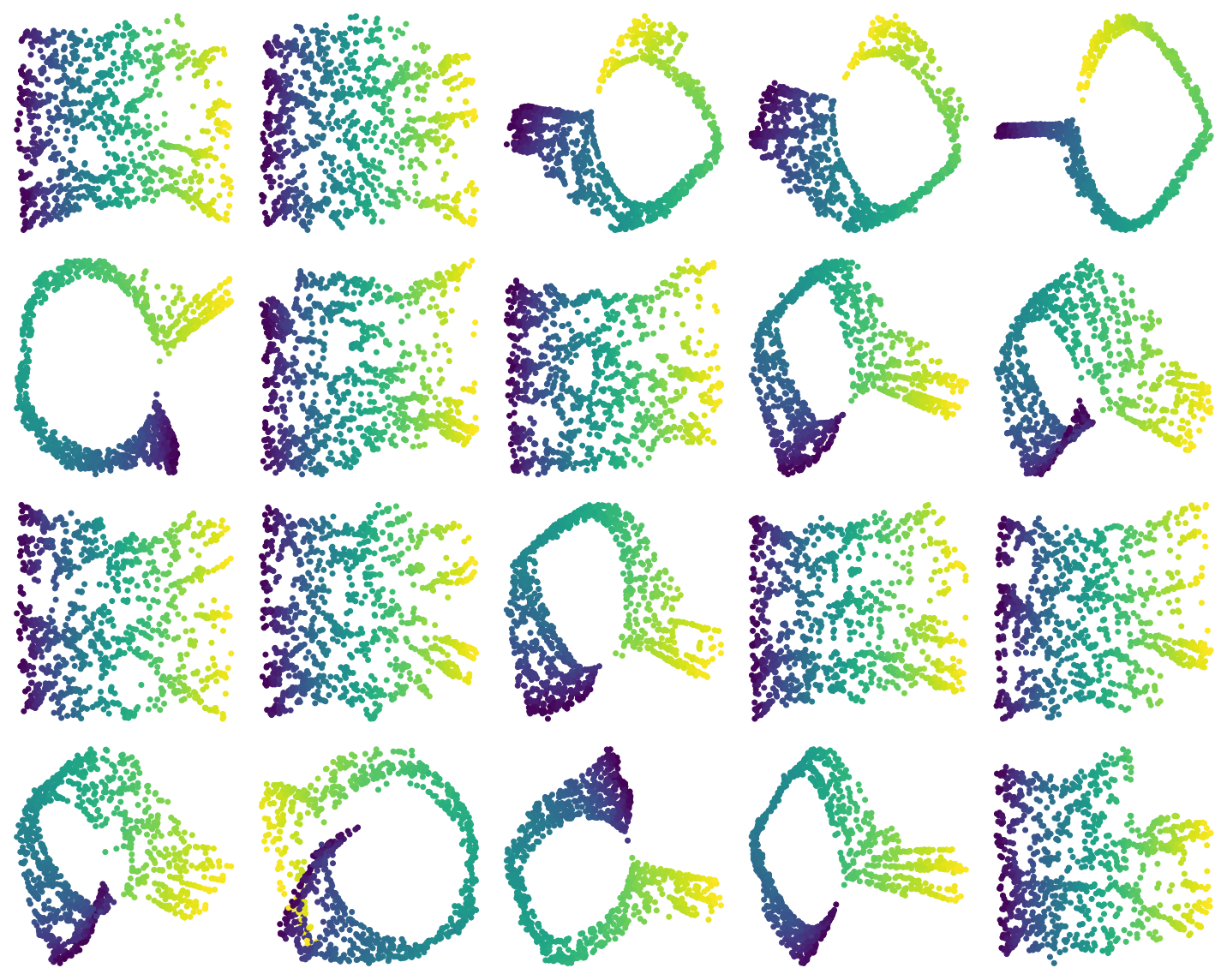
Figure 2. Some example outputs of Isomap applied to a noisy Swiss roll dataset.

The next step in the algorithm is to calculate Procrustes distances between these embeddings. We have visualized the resulting graph using multidimensional scaling MDS) in Figure 3. The two types of embeddings roughly divide into two major clusters, one consisting of unrolled sheets and one consisting of coiled up sheets. The appearance of the two clusters indicate the lack of robustness in applying Isomap to the Swiss roll with the current level of added noise. We also observe that while most unrolled outputs are close together, the coiled versions can differ greatly among themselves. (The unrolled outputs form a dense cluster while the coiled outputs do not.) The next step in the algorithm is to calculate the persistent homology of each embedding to identify the cluster consisting of the embeddings that have only very small (noise) loops in $PH_{1}$. This is precisely the cluster of the unrolled outputs.

Figure 3. An MDS representation of the Procrustes distances between Isomap outputs of 200 noisy Swiss rolls: each point represents an output, and the plot is shaded according to density of the points. Some representative points are indicated together with their corresponding Isomap embedding.

The final step is to align and average the embeddings in the unrolled cluster. The final averaged embedding is illustrated in Figure 4.

Figure 4. The Procrustes-aligned Isomap embedding corresponding to the cluster of unrolled Swiss rolls.

7.2. Robustness in presence of ambient noise concentrated around the manifold

In this experiment we simulate sampling from a data set corrupted by ambient noise. We again create a Swiss roll dataset with 2000 points. Then, we inject additive Gaussian noise to this dataset, so that Isomap produces a corrupted coiled output when run on the whole data set. See Figure 5. When we randomly subsample this dataset to obtain 500 samples of 1000 points each, for almost all of these samples the result of Isomap is a coiled embedding; only a handful are unrolled into a sheet. See Figure 6.

The next step in the algorithm is to calculate Procrustes distances between these embeddings and cluster. In this case, there are many clusters, but calculating the persistent homology of each embedding identifies a dense cluster consisting of the embeddings that have only very small (noise) loops in $PH_{1}$, in contrast to most of the clusters which are diffuse and have significant loops in $PH_{1}$. See Figure 7.

Finally, we align and average the embeddings in the unrolled cluster. The final averaged embedding is illustrated in Figure 8.

(a) The noisy swiss roll.

(b) Isomap does not return the correct embedding.

Figure 5. Additive Gaussian noise in the ambient space.

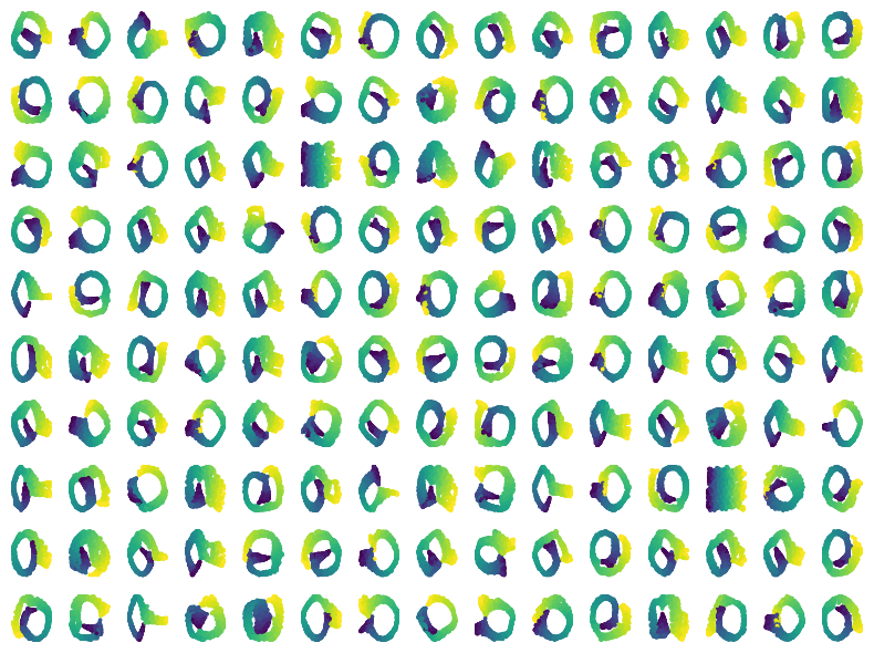
Figure 6. All but a few of the subsamples result in coiled Isomap embeddings.

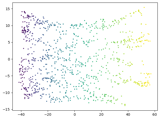
(a) One of the few subsamples resulting in an unrolled coordinate chart.

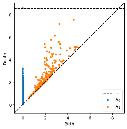
(b) The persistence diagram has a single large class in $PH_{0}$ and no large classes in $PH_{1}$.

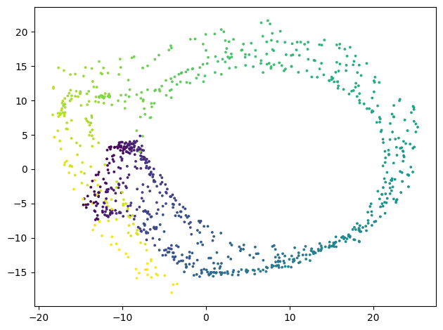
(c) A generic subsample resulting in a coiled coordinate chart.

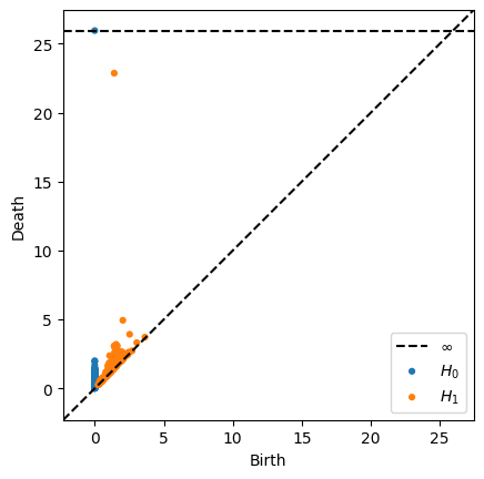
(d) The persistence diagram has a single large class in $PH_{0}$ but also has a very large class in $PH_{1}$ capturing the loop.

Figure 7. Comparing clusters in Procrustes space using persistent homology.

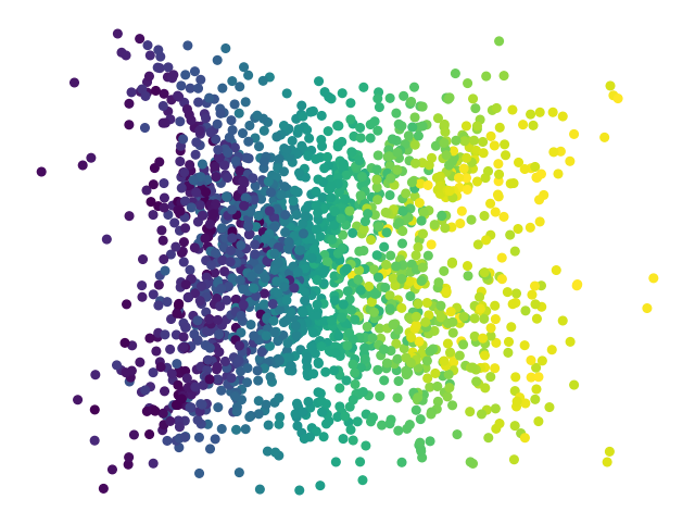
Figure 8. The Procrustes-aligned Isomap embedding corresponding to the cluster of unrolled Swiss rolls.

7.3. Robustness in presence of outliers

In these experiments, we imagine a single dataset of measurements where one or more bad sample points (“outliers”) are included. We work again with the Swiss roll. Even a single adversarial outlier can cause a short-circuit in the inferred connectivity of the manifold, and the resulting Isomap embedding will fail to unroll the Swiss roll. See Figure 9, parts 9(a) and 9(b). When we randomly subsample this dataset to obtain 200 samples of 600 points each, most of these samples do not contain the outlier, and in these cases Isomap manages to unroll the Swiss roll. See Figure 9, part 9(c). In some instances, Isomap unrolls the roll even if the outlier is included in the subsample if the other non-outlier points involved in the short-circuiting are omitted. Finally, we align all the outputs in the good cluster and compute the centroid: the result is a successfully unrolled Swiss roll. See Figure 9, part 9(d).

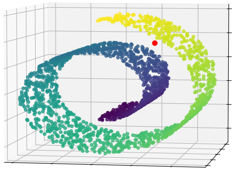
(a) Original data in 3D

(b) Isomap result

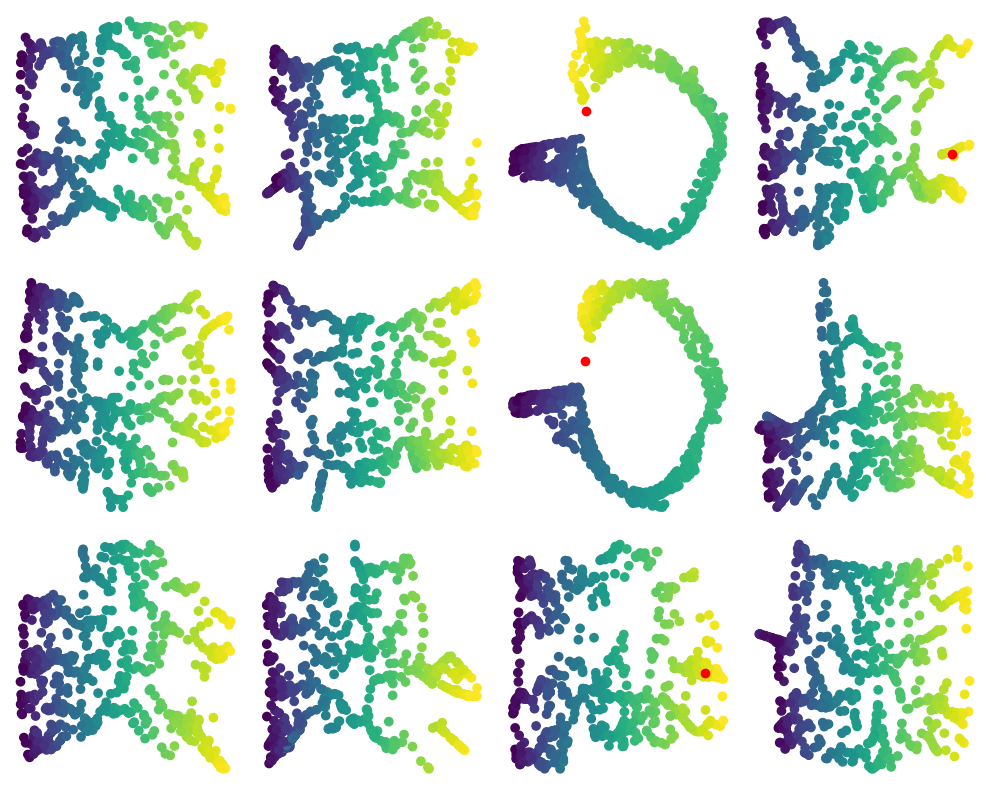
(c) Isomap applied to subsamples

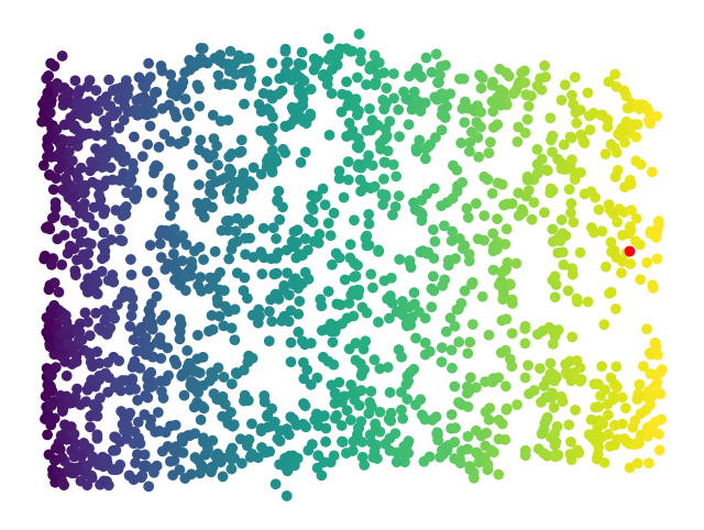
(d) Final aligned output

Figure 9. Robustifying the output of Isomap (single outlier case)

The previous experiment illustrates the need for some kind of robustification (in this case by taking subsamples) even in the presence of a single outlier. The next experiment studies the more expected case where there are multiple outliers. In this experiment, we add 100 (5%) outliers chosen uniformly from a bounding box. As in the single outlier case, we subsampled the dataset 200 times to obtain samples of size 600 and ran Isomap on these subsamples. With this many outliers, the coiled outputs are in the majority. We clustered the outputs and identified a cluster of uncoiled outputs using persistent homology. Then, we computed the Procrustes alignment and averaged over the subset of these good outputs, producing the expected unrolled Swiss roll. See Figure 10.

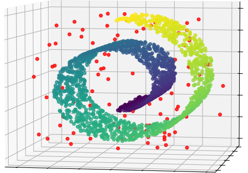
(a) Original data in 3D

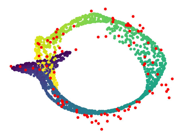
(b) Isomap result

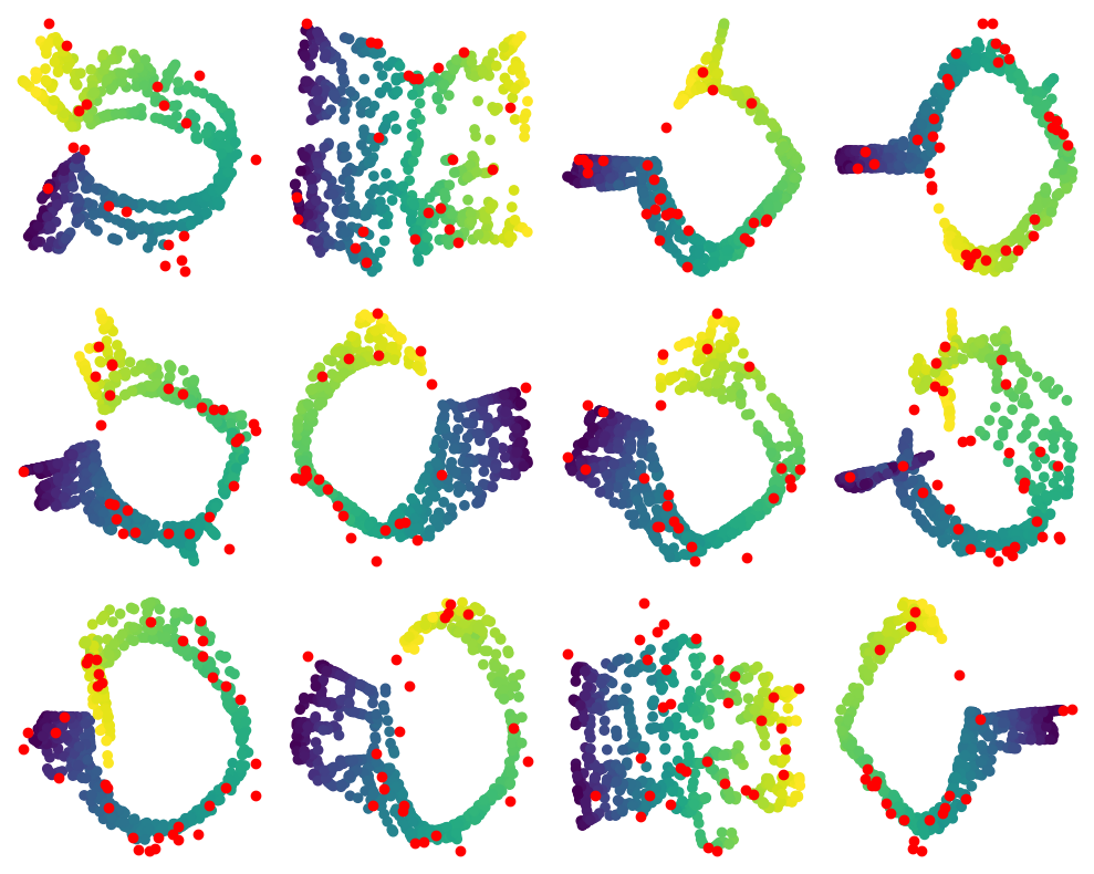
(c) Isomap applied to subsamples

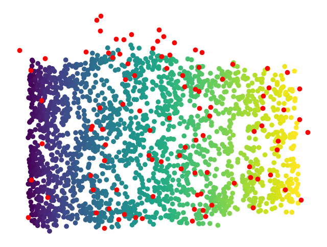
(d) Final aligned output

Figure 10. Many outliers

These experiments demonstrate that our procedure is robust to outliers, in the sense that the output in the presence of a small percentage of outliers is a low-distortion unrolled embedding of the type we expect from Isomap applied to noiseless samples from the underlying manifold.

7.4. Parameter variation

All manifold learning algorithms have hyperparameters that have to be chosen by the practitioner. In the case of Isomap, there is a single parameter corresponding to neighborhood size that needs to be judiciously chosen in order to obtain good results. The next experiment illustrates that under the hypothesis that the data represents a convex subset of a low dimensional manifold embedded in a higher dimensional manifold, we can detect a cluster of good parameters using our persistent homology methodology.

In this experiment, we apply Isomap to the 2000 point Swiss roll synthetic data set under a wide range of parameters. We have graphed the heatmap of Procrustes distances of the resulting embeddings in Figure 11. We see that at small radii, Isomap fails to find a good embedding because the points are not connected (these have high rank large bars in $PH_{0}$), whereas at large radii, the embeddings “short circuit” in the normal direction of the manifold, leading to coiled representations (these have a large bar in $PH_{1}$). Between these extremes, there is a range of values that lead to good embeddings (with no large bars in $PH_{1}$). Moreover, these embeddings are close together in Procrustes distances. Within this range, we recover the expected unrolled embedding of the Swiss roll dataset. Furthermore, there is a sharp transition between unrolled and coiled up representations, as shown by the large Procrustes distance between each embedding in the unrolled cluster and each embedding in the coiled cluster. The figure illustrates four clusters in total: the first box shows the cluster of small radii; the next 19 boxes show the cluster of unrolled embeddings; the next single box shows a transitional embedding far from both the unrolled embeddings and the coiled embeddings; and finally, the last nine boxes show the cluster of coiled embeddings. A more careful analysis of the distances (which we omit here) reveals that they correspond to the size of the gap between sheets of the roll; this is closely related to the “condition number” and reach of the manifold [23].

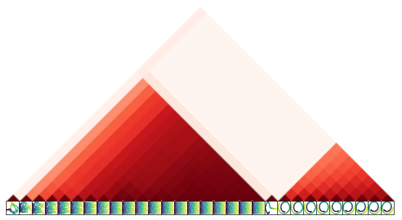
Figure 11. The Procrustes distance matrix between Isomap outputs for varying neighborhood size parameters, increasing from left to right. The output embeddings are shown along the bottom, and the triangle heatmap shows the distances: the darker the color, the smaller the Procrustes distance. (To compare two outputs: intersect the $45^{\circ}$ lines emanating from them to find the box on the heatmap illustrating their Procrustes distance.)

7.5. Detecting failure of embedding methodology

The next experiment studies a case contrary to the general hypothesis that the data comes from a convex subset of a low dimensional manifold. In this experiment, we use the vertices of buckminsterfullerene or “buckyballs” for the basic data . A buckyball is a molecule consisting of 60 carbon atoms arranged on a sphere. Its bonds forms hexagonal and pentagonal rings resembling the surface of a soccer ball. See Figure 12, part 12(a). As a proxy for the sphere $S^{2}$, the positions of the atoms of a buckyball in 3D cannot be faithfully compressed down to two dimensions, unlike the unrolling of the Swiss roll.

We computed the Isomap outputs of 500 noisy buckyballs, and the Procrustes distances between them. See Figure 12, part 12(b). We visualized these distances using MDS in Figure 12, part 12(c); however, in this case the 2-dimensional rendering obscures rather than illuminates the geometric structure of the Procrustes graph of Isomap outputs (as we explain below). Nevertheless, it illustrates enough to show that unlike in the Swiss roll studies, there are no dense clusters of embeddings in this experiment, and so we cannot expect an averaging procedure to yield a reasonable result.

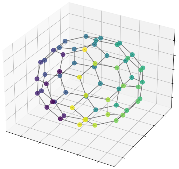
(a) Original data in 3D

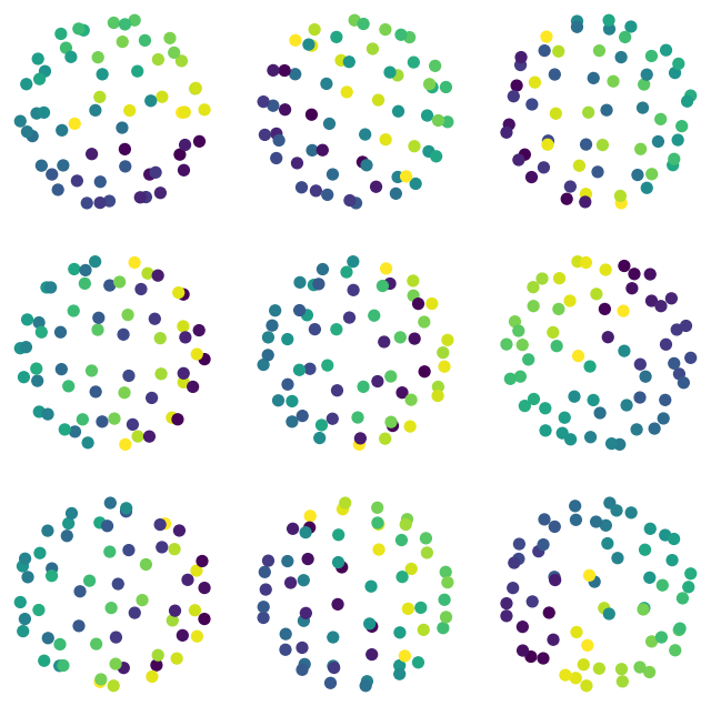
(b) Isomap of subsamples

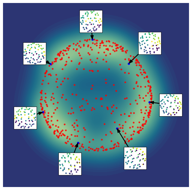
(c) MDS embedding

Figure 12. Buckyball dataset

Although not directly related to our algorithm, we can say more about the geometric structure of the Isomap outputs. We note that the typical output is approximately a flattened sphere: the dimensionality reduction algorithm is approximately linearly projecting the buckyball one dimension down. Thus, after centering the buckyball and the resulting Isomap output, we are led to consider the space $V_{2}(\mathbb{R}^{3})$ of (orthonormal) $2$-frames in $\mathbb{R}^{3}$, corresponding to the basis vectors in $\mathbb{R}^{3}$ that span the plane we are projecting to. Procrustes alignment quotients out the isometries $O(2)$ of this plane, and the Procrustes graph of outputs of Isomap on the buckyball dataset should approximate $V_{2}(\mathbb{R}^{3})/O(2)\cong\mathbb{R}P^{2}$, the real projective plane.

We can test the conclusion of this thought experiment using persistent homology. For the projective plane, using coefficient field $\mathbb{F}_{p}$, $p$ prime,

$$H_{1}(\mathbb{R}P^{2};\mathbb{F}_{p})\cong H_{2}(\mathbb{R}P^{2};\mathbb{F}_{p})\cong\begin{cases}\mathbb{F}_{2},&\text{if }p=2\\ 0,&\text{if }p>2.\end{cases}$$

Computing the persistent homology for the point cloud consisting of the 500 Isomap outputs with the Procrustes metric with Ripser [31], we find persistent classes in $PH_{1}(\mathbb{R}P^{2};\mathbb{F}_{2})$ and $PH_{2}(\mathbb{R}P^{2};\mathbb{F}_{2})$, but not in $PH_{*}(\mathbb{R}P^{2};\mathbb{F}_{p})$ for $p=3$ or $5$. See Figure 13. In other words, the persistent homology signature of the Isomap outputs matches the prediction that the landscape of Isomap outputs at least homotopically is an approximation of $\mathbb{R}P^{2}$.

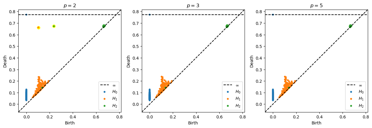
Figure 13. Persistence diagrams for the Procrustes graph of Isomap outputs for the buckyball dataset

7.6. Divide and conquer for very large data sets

Manifold learning algorithms tend to have superlinear time complexity. This suggests that using a divide-and-conquer approach on large datasets may result in time savings. The idea is the same as before: subsample the dataset, run the algorithm on the individual subsamples, and then use the Procrustes alignment to merge the results. A schematic of this process is shown in Figure 14.

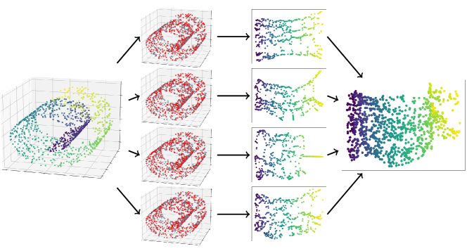
Figure 14. Starting with a large dataset, repeatedly subsample the dataset to obtain multiple subsamples of smaller size (here the subsamples are indicated in red). Then, apply the manifold learning algorithm to each subsample and use the Procrustes alignment to average the resulting embeddings.

8. Analysis of real data coming from single-cell genomics

The purpose of this section is to explore an application of our algorithm to real data. We use two data sets as examples where coordinates in dimensionality-reduced genomic space allows us to determine cell types. The first such data set comes from blood cells (PBMC) and the second from mouse neural tissue (Tabula muris). In these applications, in addition to Isomap, we use four other manifold learning (dimensionality reduction) algorithms: PCA, Laplacian eigenmaps, t-SNE, and UMAP. In each case, we look at coordinates resulting from applying just the dimensionality reduction algorithm (“base case”) and our algorithm (“robustified case”).

We see interesting new phenomena in these applications. For one thing, using the manifold learning algorithms PCA, Laplacian eigenmaps, and Isomap with our algorithm, we see a single large tight cluster in the Procrustes graph of the subsamples. However, unlike the charts for the synthetic Swiss roll examples, both the good and the bad embeddings have trivial $PH_{1}$, our indicator for contractibility. Instead, what distinguishes the good from the bad embeddings is how evenly spread they are. We used embeddings in $\mathbb{R}^{2}$ and the bad embeddings are ones concentrated along a single axis, being approximately one-dimensional, whereas the good embeddings have extent in both dimensions. For both theoretical and practical reasons (as explained in the discussion of the algorithm), the embeddings that are essentially one-dimensional need to be discarded.

On the other hand, using t-SNE and UMAP, the Procrustes graph of the subsamples are comparatively very spread out and form a single large but extremely spread out cluster, indicating that the averaging procedure in our algorithm cannot be expected to output reasonable coordinates. This dichotomy is not surprising since the PCA, Laplacian eigenmaps, and Isomap algorithms strive to perform global alignment of the local coordinates, whereas the t-SNE and UMAP algorithms are designed to separate local clusters. (This dichotomy of behavior is a topic of interest in the genomics methodology community, see for example [30] for a critical review of the use of these kinds of dimensionality reduction to produce pictures.)

8.1. 3k PBMCs scRNA-sequencing

The first dataset is a preprocessed version of single cell RNA-sequencing data from 3k peripheral blood mononuclear cells (PBMCs) from a healthy donor, made freely available by 10x Genomics. Comprised of cells from a variety of myeloid and lymphoid lineages, the dataset has rich cluster and continuous structure, making it a useful dataset to benchmark new bioinformatic methods. It can be accessed using the scanpy Python package [35] via the following command:

scanpy.datasets.pbmc3k_processed

As is typical in the visualization of scRNA-sequencing data, PCA is used as a preliminary step prior to constructing the 2D embeddings: we reduce the raw data to the first 50 principal components. For the base case, we then applied each of the manifold learning algorithms to reduce the coordinates in $\mathbb{R}^{50}$ to $\mathbb{R}^{2}$. For the robustified case, we take 50 subsamples of 500 cells, and proceed with our algorithm with each of the manifold learning algorithms used for dimensionality reduction from $\mathbb{R}^{50}$ to $\mathbb{R}^{2}$.

Figure 15 shows the MDS plots of the Procrustes distances between the subsample embeddings along with histograms of those values under each of the five manifold learning algorithms. We can see that PCA, Laplacian eigenmaps, Isomap have much more concentrated Procrustes distances. And when we look at the MDS plot of the Procrustes distances, we see there are tight clusters of the embeddings, whereas the embeddings for t-SNE and UMAP are significantly more spread out (with a diameter over 4 times as large). The algorithm then proceeds for PCA, Laplacian eigenmaps, Isomap and terminates with an error of no remaining clusters for t-SNE and UMAP.

For PCA, Laplacian eigenmaps, Isomap we find that the main cluster has embeddings that are essentially two-dimensional; the outlying points are the embeddings that are essentially one-dimensional. In Figures 16 and  17 we plot the subsample embeddings for PCA and Isomap. (The relatively larger number of bad embeddings for PCA in Figure 16 versus Isomap in 17 is consistent with the larger number of embeddings outside the tight cluster as pictured in Figure 15.) We select the good cluster and apply averaging procedure to the subsample embeddings it contains. The output is robustified coordinates for PCA, Laplacian eigenmaps, and Isomap. This is illustrated in Figure 18 together with the embeddings obtained on the entire data set. In the figure, the data points are colored by cell type.

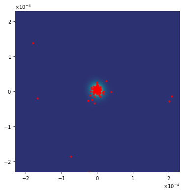
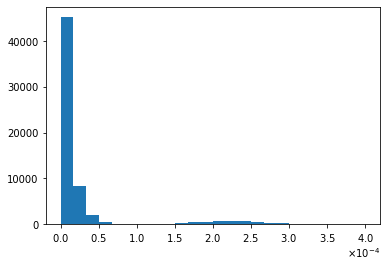
(a) PCA

(b) Isomap

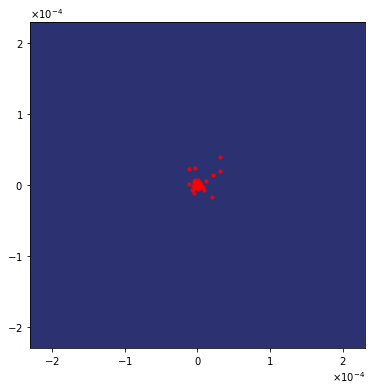
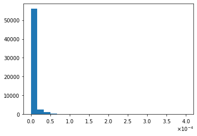
(c) Laplacian eigenmaps.

(d) t-SNE.

(e) UMAP.

Figure 15. Procrustes distances between subsample embeddings for the PBMC dataset.

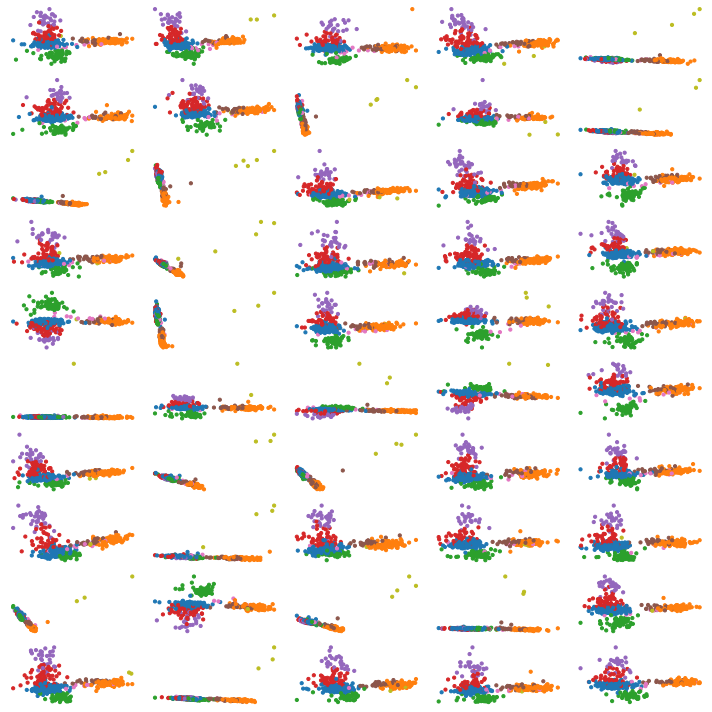
Figure 16. Subsample embeddings from PCA.

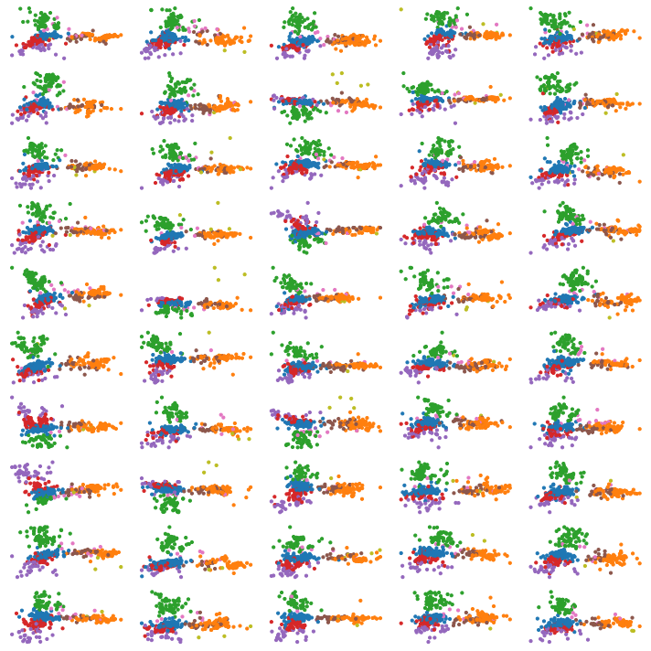
Figure 17. Subsample embeddings from Isomap.

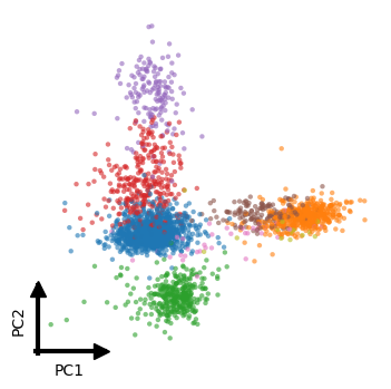
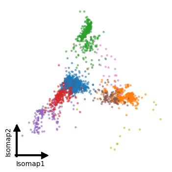
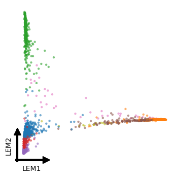
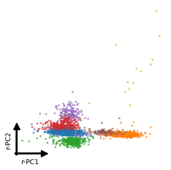
(a) PCA

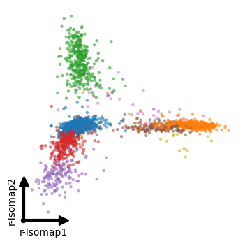
(b) Isomap

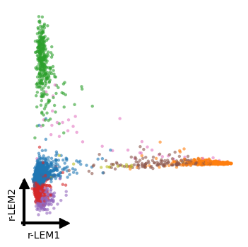
(c) Laplacian Eigenmaps

Figure 18. Original and robustified embeddings for the PBMC dataset.

8.2. The mouse brain from Tabula muris

The second dataset is another single cell RNA-sequencing dataset, this time coming from the Tabula muris project [10], sequenced using the Smart-seq2 protocol, which we downsample to the 7,249 non-myeloid cells in the brain tissue sample. According to the provided cell type annotation, this sample contains a mixture of neurons as well as glial cells. We perform the same experimental protocol as above on the PBMC data set, and find similar conclusions, except that in this case Isomap gives a significantly more diffuse cluster in Procrustes space than PCA or Laplacian eigenmaps, and seems to give as poor a performance as t-SNE and UMAP. See figures 19 and 20.

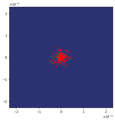
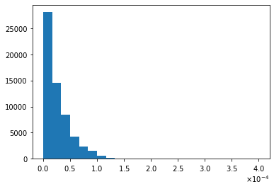
(a) PCA

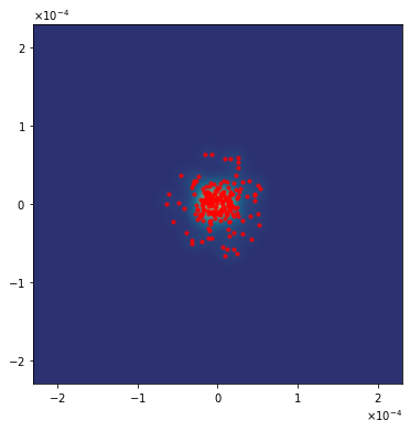
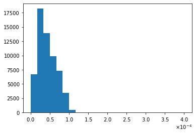
(b) Isomap

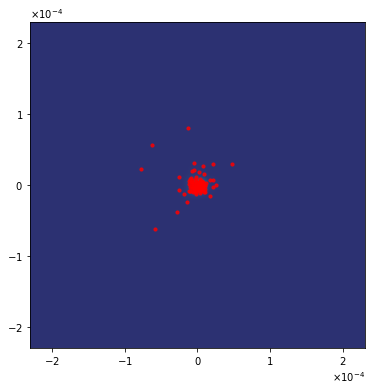
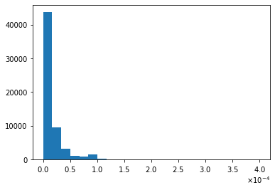
(c) Laplacian eigenmaps.

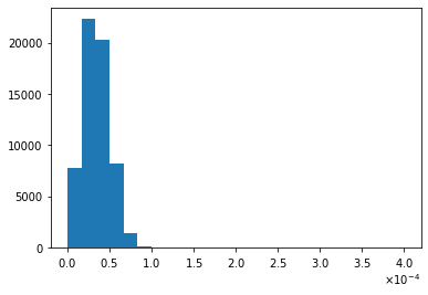
(d) t-SNE.

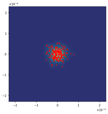
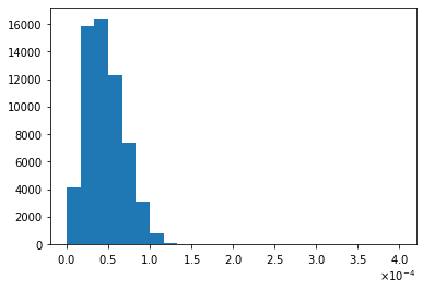
(e) UMAP.

Figure 19. Procrustes distances between subsample embeddings for the TM dataset.

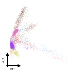
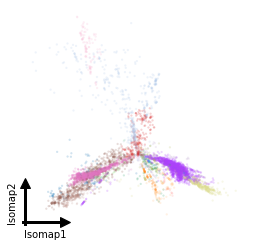
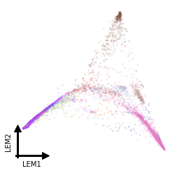
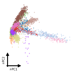
(a) PCA

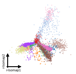
(b) Isomap

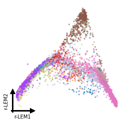
(c) Laplacian Eigenmaps

Figure 20. Original and robustified embeddings for the TM dataset.

References

- [1] Jose Manuel Andrade, Marı́a P. Gómez-Carracedo, Wojtek Krzanowski and Mikael Kubista “Procrustes rotation in analytical chemistry, a tutorial” In Chemometrics and Intelligent Laboratory Systems 72.2, 2004, pp. 123–132 DOI: https://doi.org/10.1016/j.chemolab.2004.01.007
- [2] Angela Andreella and Livio Finos “Procrustes Analysis for High-Dimensional Data” In Psychometrika 87.4, 2022, pp. 1422–1438 DOI: 10.1007/s11336-022-09859-5
- [3] Mukund Balasubramanian and Eric L. Schwartz “The Isomap Algorithm and Topological Stability” In Science 295.5552, 2002, pp. 7 DOI: 10.1126/science.295.5552.7a
- [4] Juan Antonio Balbuena, Raul Miguez-Lozano and Isabel Blasco-Costa “PACo: A Novel Procrustes Application to Cophylogenetic Analysis” In PLOS ONE 8.4 Public Library of Science, 2013, pp. 1–15 DOI: 10.1371/journal.pone.0061048
- [5] Jos M.. Berge “Orthogonal Procrustes rotation for two or more matrices” In Psychometrika 42.2, 1977, pp. 267–276
- [6] Jos M.. Berge, Henk A.. Kiers and Jacques J.. Commandeur “Orthogonal Procrustes rotation for matrices with missing values” In British J. Math. Statist. Psych. 46.1, 1993, pp. 119–134 DOI: 10.1111/j.2044-8317.1993.tb01005.x
- [7] Andrew J. Blumberg, Itamar Gal, Michael A. Mandell and Matthew Pancia “Robust Statistics, Hypothesis Testing, and Confidence Intervals for Persistent Homology on Metric Measure Spaces” In Found. Comput. Math. 14.4, 2014, pp. 745–789
- [8] Fred L. Bookstein “Morphometric Tools for Landmark Data: Geometry and Biology” Cambridge University Press, 1992 DOI: 10.1017/CBO9780511573064
- [9] Jacques J.. Commandeur “Matching configurations” DWSO Press, 1991
- [10] The Tabula Muris Consortium “A single-cell transcriptomic atlas characterizes ageing tissues in the mouse” In Nature 583, 2020, pp. 590–595 DOI: 10.1038/s41586-020-2496-1
- [11] Garmt Dijksterhuis “Multivariate data analysis in sensory and consumer science: an overview of developments” In Trends in Food Science & Technology 6.6, 1995, pp. 206–211 DOI: 10.1016/S0924-2244(00)89056-1
- [12] C.. Glasbey and K.. Mardia “A review of image-warping methods” In Journal of Applied Statistics 25.2, 1998, pp. 155–171 DOI: 10.1080/02664769823151
- [13] Colin Goodall “Procrustes Methods in the Statistical Analysis of Shape” In Journal of the Royal Statistical Society: Series B (Methodological) 53.2, 1991, pp. 285–321 DOI: 10.1111/j.2517-6161.1991.tb01825.x
- [14] J.C. Gower “Generalized Procrustes analysis” In Psychometrika 40.1, 1975, pp. 33–51 DOI: 10.1007/BF02291478
- [15] John C. Gower and Garmt B. Dijksterhuis “Multivariate analysis of coffee images: A study in the simultaneous display of multivariate quantitative and qualitative variables for several assessors” In Quality and Quantity 28.2, 1994, pp. 165–184 DOI: 10.1007/BF01102760
- [16] B.F. Green “The orthogonal approximation of an oblique structure in factor analysis” In Psychometrika 17.4, 1952, pp. 429–440 DOI: 10.1007/BF02288918
- [17] David G. Kendall “Shape Manifolds, Procrustean Metrics, and Complex Projective Spaces” In Bulletin of the London Mathematical Society 16.2, 1984, pp. 81–121 DOI: 10.1112/blms/16.2.81
- [18] S.. Langron and A.. Collins “Perturbation Theory for Generalized Procrustes Analysis” In Journal of the Royal Statistical Society. Series B (Methodological) 47.2 [Royal Statistical Society, Oxford University Press], 1985, pp. 277–284
- [19] Jan Leeuw and Jacqueline Meulman “A special jackknife for multidimensional scaling” In Journal of Classification 3.1, 1986, pp. 97–112 DOI: 10.1007/BF01896814
- [20] Francy Junio Gonçalves Lisboa et al. “Much beyond Mantel: Bringing Procrustes Association Metric to the Plant and Soil Ecologist’s Toolbox” In PLOS ONE 9.6 Public Library of Science, 2014, pp. 1–9 DOI: 10.1371/journal.pone.0101238
- [21] Rong Ma, Eric D. Sun, David Donoho and James Zou “Principled and interpretable alignability testing and integration of single-cell data” In Proceedings of the National Academy of Sciences 121.10, 2024 DOI: 10.1073/pnas.2313719121
- [22] A.D. McLachlan “A mathematical procedure for superimposing atomic coordinates of proteins” In Acta Crystallographica Section A 28.6, 1972, pp. 656–657 DOI: 10.1107/S0567739472001627
- [23] Partha Niyogi, Stephen Smale and Shmuel Weinberger “Finding the Homology of Submanifolds with High Confidence from Random Samples” In Discrete and Computational Geometry 39, 2008, pp. 419–441
- [24] Michael B. Richman and Stephen J. Vermette “The use of Procrustes Target Analysis to discriminate dominant source regions of fine sulfur in the western U.S.A.” In Atmospheric Environment. Part A. General Topics 27.4, 1993, pp. 475–481 DOI: https://doi.org/10.1016/0960-1686(93)90205-D
- [25] Peter H. Schönemann “A generalized solution of the orthogonal Procrustes problem” In Psychometrika 31.1, 1966, pp. 1–10 DOI: 10.1007/BF02289451
- [26] Peter H. Schönemann and Robert M. Carroll “Fitting one matrix to another under choice of a central dilation and a rigid motion” In Psychometrika 35.2, 1970, pp. 245–255 DOI: 10.1007/BF02291266
- [27] Robin Sibson “Studies in the Robustness of Multidimensional Scaling: Perturbational Analysis of Classical Scaling” In Journal of the Royal Statistical Society. Series B (Methodological) 41.2 [Royal Statistical Society, Wiley], 1979, pp. 217–229 URL: http://www.jstor.org/stable/2985036
- [28] Inge Söderkvist “Perturbation analysis of the orthogonal Procrustes problem” In BIT 33.4, 1993, pp. 687–694 DOI: 10.1007/BF01990543
- [29] G.. Stewart “Perturbation theory for the singular value decomposition” UMIACS-TR-90-124, 1998
- [30] Chari T. and Pachter L. “The specious art of single-cell genomics” In PLoS Comput Biol 19.8, 2023 URL: https://doi.org/10.1371/journal.pcbi.1011288
- [31] Christopher Tralie, Nathaniel Saul and Rann Bar-On “Ripser.py: A Lean Persistent Homology Library for Python” In The Journal of Open Source Software 3.29, 2018, pp. 925 DOI: 10.21105/joss.00925
- [32] Pauli Virtanen et al. “SciPy 1.0: Fundamental Algorithms for Scientific Computing in Python” In Nature Methods 17, 2020, pp. 261–272 DOI: 10.1038/s41592-019-0686-2
- [33] Chang Wang and Sridhar Mahadevan “Manifold alignment using Procrustes analysis” In Proceedings of the 25th International Conference on Machine Learning, 2008, pp. 1120–1127 DOI: 10.1145/1390156.1390297
- [34] Chaolong Wang et al. “Comparing Spatial Maps of Human Population-Genetic Variation Using Procrustes Analysis” In Statistical Applications in Genetics and Molecular Biology 9.1, 2010 DOI: doi:10.2202/1544-6115.1493
- [35] F. Wolf, Philipp Angerer and Fabian J. Theis “SCANPY: large-scale single-cell gene expression analysis” In Genome Biology 19.15, 2018 DOI: 10.1186/s13059-017-1382-0