A Tiny Supervised ODL Core with Auto Data Pruning for Human Activity Recognition

Abstract

In this paper, we introduce a low-cost and low-power tiny supervised on-device learning (ODL) core that can address the distributional shift of input data for human activity recognition. Although ODL for resource-limited edge devices has been studied recently, how exactly to provide the training labels to these devices at runtime remains an open-issue. To address this problem, we propose to combine an automatic data pruning with supervised ODL to reduce the number queries needed to acquire predicted labels from a nearby teacher device and thus save power consumption during model retraining. The data pruning threshold is automatically tuned, eliminating a manual threshold tuning. As a tinyML solution at a few mW for the human activity recognition, we design a supervised ODL core that supports our automatic data pruning using a 45nm CMOS process technology. We show that the required memory size for the core is smaller than the same-shaped multilayer perceptron (MLP) and the power consumption is only 3.39mW. Experiments using a human activity recognition dataset show that the proposed automatic data pruning reduces the communication volume by 55.7% and power consumption accordingly with only 0.9% accuracy loss.

1 Introduction

In practical edge AI scenarios, data distribution around edge devices may vary depending on a given environment. Such data distribution shift is known as data drift and is a major challenge for edge AI. It is likely that each edge device cannot access all the data and hence data distribution is biased depending on the environment. In the case of human activity recognition, data distribution varies depending on human subjects. Figure 1 shows dimensionality reduction results of a human activity recognition dataset that contains samples obtained from 30 human subjects [1]. There are six classes in the dataset: Walking, Walking upstairs, Walking downstairs, Sitting, Standing, and Laying. Samples obtained from the same human subject are plotted with the same color, while numbers in the graphs are the IDs of some selected human subjects. As shown in the leftmost graph, the samples from the same human subjects form clusters during Walking. A similar tendency is observed for the Walking upstairs, Walking downstairs, and Laying classes. As mentioned above, it is likely that an edge device cannot access the samples from all the human subjects at the design time. In this case, an edge AI model that has been optimized for a specific human subject may not work well for different human subjects that have not been considered yet.

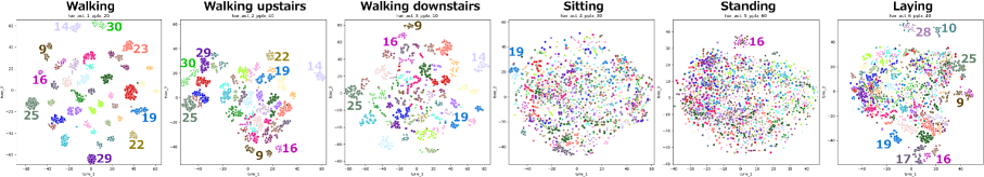
Figure 1: 2-D visualization results of 6-class human activity recognition dataset that contains samples obtained from 30 human subjects [1].

In this paper, we introduce a low-cost and low-power tiny supervised ODL core to address the above-mentioned data drift issue for the human activity recognition. Although neural network ODLs for resource-limited edge devices have been studied recently [2, 3, 4, 5], how exactly to provide the training labels to the edge devices at runtime for classification tasks remains an open-issue. For example, the authors of [4] only mention that they enable the onboard online post-training for 2,000 iterations via Bluetooth. To address this labeling issue, the edge devices can query a nearby teacher device (e.g., mobile computer) wirelessly to acquire labels and retrain the model. However, the problem with this approach is the redundant queries to the teacher that can waste wireless communication power. In this paper, we propose a new approach to reduce the redundant wireless communication of the supervised ODL between the teacher and edge devices.

2 Supervised ODL with Auto Pruning

Figure 2(a) illustrates the overall system consisting of a single teacher and multiple edge devices. Each edge device incorporates the proposed supervised ODL core. We assume that the teacher is a mobile computer that has an ensemble of highly accurate models. Edge devices send the input data to the teacher and receive a predicted label from the teacher.

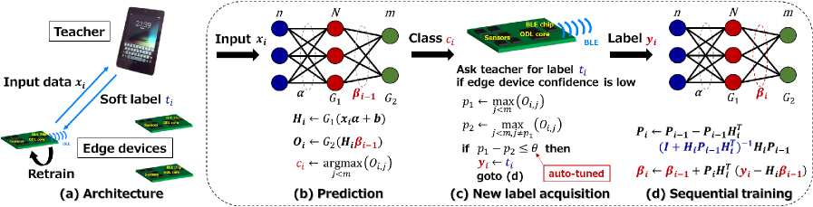
Figure 2: Proposed supervised ODL system. (a) illustrates the overall system consisting of a single teacher and multiple edge devices, where $\bm{x_{i}}\in\mathbb{R}^{n}$ and $t_{i}$ are $n$-dimensional input data and corresponding predicted label from teacher at time $i$. (b) illustrates the prediction algorithm at edge devices, where $n$, $N$, and $m$ are numbers of input, hidden, and output layer nodes. $\bm{\alpha}\in\mathbb{R}^{n\times N}$ denote weight parameters between input and hidden layers, and $\bm{\beta_{i-1}}\in\mathbb{R}^{N\times m}$ denote those between hidden and output layers trained at time $i-1$. $G_{1}$ and $G_{2}$ are activation functions of hidden and output layers. $\bm{H_{i}}\in\mathbb{R}^{N}$ and $\bm{O_{i}}\in\mathbb{R}^{m}$ are their outputs at time $i$. Particularly, $O_{i,j}$ denotes probability of $j$-th class, and $c_{i}$ is predicted class at time $i$. (c) illustrates our label acquisition algorithm, where $p_{1}$ and $p_{2}$ denote probabilities of top2 labels, and $\bm{y_{i}}\in\mathbb{R}^{m}$ is one-hot encoded label at time $i$. $\theta$ can be auto-tuned. (d) illustrates the sequential training algorithm, where $\bm{\beta_{i}}\in\mathbb{R}^{N\times m}$ denote new weights updated at time $i$. $\bm{P_{i}}\in\mathbb{R}^{N\times N}$ denote temporary values needed to compute $\bm{\beta_{i}}$.

Algorithm 1 shows the top-level function of the edge devices; this function is called periodically (e.g., once per second) by the edge devices. Assume that one of the edge devices in Figure 2(a) collects some sensor data $\bm{x_{i}}$ at time $i$ (Line 1). The next step depends on the operation mode of the ODL core: predicting or training mode. An ODL algorithm based on neural networks is used to update their weight parameters in the training mode. Section 2.1 describes the ODL algorithm (Lines 6 and 9). Section 2.2 describes our label acquisition approach (Line 8) via the teacher device and automatic data pruning to reduce communication. The operation modes are switched by a data drift detection algorithm (Line 3). Existing data drift detection algorithms [6] can be used by considering expected data drift types such as sudden drift, gradual drift, incremental drift, and reoccurring drift. The training finishes when a prespecified condition, such as the number of required training samples or training loss, is satisfied (Line 10). Finally, Section 2.3 describes the design of the proposed tiny supervised ODL core.

Algorithm 1 Top-level function (at time $i$) of our ODL core.

1:$\bm{x_{i}}\leftarrow$ Sense()

2:if mode = predicting then

3:     if IsDrift($\bm{x_{i}}$) then

4:         mode $\leftarrow$ training

5:     end if

6:     return Predict($\bm{x_{i}}$) $\triangleright$ Figure 2(b)

7:else if mode = training then

8:     $\bm{y_{i}}\leftarrow$ LabelAcquire(Predict($\bm{x_{i}}$)) $\triangleright$ Figure 2(c)

9:     SequentialTrain($\bm{x_{i}}$, $\bm{y_{i}}$) $\triangleright$ Figure 2(d)

10:     if IsTrainDone() then

11:         mode $\leftarrow$ predicting

12:     end if

13:end if

2.1 ODL Algorithm

To enable ODL on resource-limited edge devices, we utilize the OS-ELM algorithm in [7]. OS-ELM assumes simple neural networks that consist of input, hidden, and output layers, as shown in Figure 2(b). The weight parameters between the input and hidden layers are denoted as $\bm{\alpha}$, while those between the hidden and output layers are denoted as $\bm{\beta}$. $\bm{\alpha}$ are initialized with random values at the startup time, while $\bm{\beta}$ are sequentially updated by input data $\bm{x}$ and labels $\bm{y}$. Figure 2(d) shows the sequential training algorithm of OS-ELM. At time $i$, $\bm{\beta_{i}}$ are calculated and updated by $\bm{x_{i}}$, $\bm{y_{i}}$, previous weight parameters $\bm{\beta_{i-1}}$, and temporary values $\bm{P_{i}}$. As shown in the figure, $\bm{P_{i}}$ are derived from the previous values $\bm{P_{i-1}}$ and $\bm{H_{i}}$, which are hidden-layer outputs based on $\bm{x_{i}}$.

2.2 Label Acquisition with Auto Data Pruning

Since proper labeling is mandatory to correctly train the model in a short time, we exploit the nearby teacher device via BLE; that is, the edge devices send input data $\bm{x_{i}}$ to the nearby teacher and receive a predicted label $t_{i}$ from the teacher, as shown in Figure 2(c). $t_{i}$ is then converted to a one-hot encoded label $\bm{y_{i}}$. If such a nearby teacher is not available, the queries to the teacher will be retried later or skipped. The problem with this approach is the excessive number of queries to the teacher that can waste wireless communication power.

We propose to use data pruning that suppresses excessive queries combined with the supervised ODL. In our label acquisition approach, if the conditions below are met:

1. A pre-specified number of samples has been trained,

2. Data drift is not currently detected, and

3. Confidence of the predicted label is high,

then the edge devices do not need to query a teacher, and thus they can skip the sequential training. The first and second conditions confirm that a data distribution did not change during this training phase. As for the third condition, in this paper, our edge devices predict locally using the current weights being trained to produce the first and second highest probabilities $p_{1}$ and $p_{2}$ of top2 labels, as shown in Figure 2(c). Then, their difference $p_{1}-p_{2}$ is used as a confidence metric, which is denoted as “P1P2” in this paper. That is, the third condition is satisfied if $p_{1}-p_{2}>\theta$. $\theta$ is a tuning parameter, and a manual tuning of $\theta$ by sweeping many possible values is impractical. To properly choose $\theta$ at runtime,

1. $\theta$ is set to a high value at the startup time;

2. $\theta$ is then gradually decreased if the following condition is $X$ times consecutively satisfied: $p_{1}-p_{2}>\theta$ or $c=t$ when querying ($p_{1}-p_{2}\leq\theta$), where $c$ is locally-predicted label and $t$ is teacher’s predicted label;

3. $\theta$ is increased if $c\neq t$ when querying ($p_{1}-p_{2}\leq\theta$).

2.3 ODL Core Design

As a tinyML solution at a few mW for the human activity recognition, the proposed ODL core including the prediction, label acquisition, and sequential training is designed with Verilog HDL. The number of input layer nodes $n$, hidden layer nodes $N$, and output layer nodes $m$ can be customized; for example, they are set to 561, 128, and 6 in our prototype implementation. This ODL core is flexible. Because the multiply-add and division units are controlled by a state machine for the prediction, label acquisition, and sequential training, $n$, $N$, and $m$ can be changed at the startup time depending on applications as long as the on-chip SRAM capacity allows it.

In OS-ELM, random values are stored as $\bm{\alpha}$ [7]. To reduce the memory size of $\bm{\alpha}$, the weights can be replaced with a pseudorandom number generator as in [8]. We also follow this direction and hence examine the following variants:

• ODLBase: 32-bit random numbers are stored as weights $\bm{\alpha}$.

• ODLHash: $\bm{\alpha}$ are replaced with a 16-bit Xorshift function, where coefficients are 7, 9, and 8.

Table 1: Memory size of ODL cores [kB] ($n$ = 561 and $m$ = 6).

$N$	32	64	128	256	512
NoODL	74.82	147.40	292.55	582.85	1163.46
ODLBase	83.01	180.16	423.62	1107.14	3260.61
ODLHash	11.20	36.55	136.39	532.68	2111.68

Table 2: Comparisons with reported results.

	# of parameters	Accuracy [%]
ODLHash ($N$ = 128)	34k	93.67
ODLHash ($N$ = 256)	133k	95.51
Q. Teng et al., [9]	0.35M	96.98
W. Huang et al., [10]	0.84M	97.28

Table 1 shows their total memory sizes $M_{bit}$ when $N$ is varied from 32 to 512 assuming that $n$ and $m$ are 561 and 6, respectively. “NoODL” means the same MLP as in ODLBase, but without the ODL capability. As shown in the table, $M_{bit}$ is significantly reduced by ODLHash compared with ODLBase especially when $N$ is less than or equal to 256. It is interesting that in these cases ODLHash is smaller than NoODL.

Table 2 compares ODLHash with results reported in [9, 10] in terms of the parameter size and classification accuracy for the human activity recognition dataset [1]. Our ODLHash achieves favorable accuracies compared with these SOTA results even with very small parameter sizes (e.g., ODLHash when $N$ is 128 is an order of magnitude smaller than [9] and [10]). More importantly, ODLHash has the ODL capability (thus including the temporary storage for ODL) which is a big advantage when it is deployed at environments where data distribution may change, as demonstrated in the next section.

3 Evaluations

The proposed ODL approaches are evaluated in terms of the classification accuracy using a data drift dataset. The human activity recognition dataset [1] is modified to create shifted datasets before and after a data drift. Specifically, based on the dimensionality reduction results (Figure 1), samples obtained from human subjects 9, 14, 16, 19, and 25 are removed from the original training and test datasets, and these reduced training and test datasets are used as training and “test0” datasets in this paper. Those of human subjects 9, 14, 16, 19, and 25 are used as “test1” dataset. Labels of these datasets are used as teacher’s predicted labels (i.e., $t_{i}$ in Figure 2(c)).

Table 3: Accuracy of ODL approaches and counterparts before and after drift.

	Before [%]	After [%]
NoODL ($N$ = 128)	92.9$\pm$0.8	82.9$\pm$1.4
ODLBase ($N$ = 128)	93.4$\pm$0.6	90.8$\pm$1.7
ODLHash ($N$ = 128)	93.1$\pm$0.8	90.7$\pm$1.0
NoODL ($N$ = 256)	95.1$\pm$0.3	83.7$\pm$1.0
ODLBase ($N$ = 256)	95.2$\pm$0.3	92.5$\pm$0.6
ODLHash ($N$ = 256)	95.1$\pm$0.4	92.3$\pm$0.7
DNN (561,512,256,6)	94.1$\pm$1.0	85.2$\pm$1.3

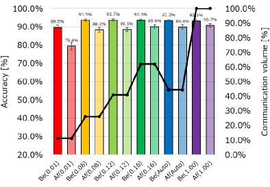
Figure 3: Communication volume with different $\theta$.

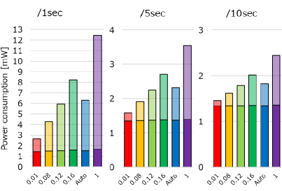
Figure 4: Power consumption with different $\theta$.

The following steps are executed 20 times for each approach to report their test accuracies before and after the data drift:

1. Initial training: Models are trained with the training dataset.

2. Test before drift: Models are tested with the test0 dataset.

3. ODL: Models are retrained with approximately 60% of the test1 dataset. This step is not executed in NoODL.

4. Test after drift: Models are tested with the remaining samples of the test1 dataset.

3.1 ODL Approaches vs. NoODL

The proposed ODL approaches and counterparts are evaluated in terms of the classification accuracy. Table 3 shows the mean and standard deviation of the test accuracies before and after the data drift. “DNN” is a simple MLP that has two hidden layers. The accuracies tend to be high when $N$ is large, and they are almost saturated when $N$ is 256. Although the accuracies when $N$ is 128 are slightly lower than those when $N$ is 256, the memory sizes when $N$ is 256 are significantly large compared with those when $N$ is 128; for example, the memory size of ODLHash is increased by 3.91$\times$ as $N$ is increased from 128 to 256, as shown in Table 1. We thus focus on ODL approaches when $N$ is 128 since they can strike a good balance between the accuracy and memory size as low-end tinyML solutions. In NoODL, the accuracy drops after the data drift, while the accuracy is recovered in ODLBase and ODLHash. ODLHash achieves almost the same accuracies as ODLBase. These results demonstrate benefits of our supervised ODL in data drift situations.

3.2 Data Pruning with Different Thresholds

The proposed ODLHash with the data pruning (P1P2) is evaluated in terms of the classification accuracy and communication volume by varying the confidence threshold $\theta$. $N$ is set to 128. $\theta$ is varied from 0.01 to 1 (no data pruning when $\theta$ = 1). The experiments are executed 20 times for each configuration. The number of initial samples to be trained before the data pruning is enabled (i.e., condition 1 of Section 2.2) is empirically determined by max($N$, 288).

In Figure 4, bar graphs show the mean and standard deviation of the test accuracies before and after the data drift. “Be” and “Af” indicate those of ODLHash before and after the data drift. “Auto” indicates the proposed auto-tuning of $\theta$. As expected, the accuracies tend to be low when $\theta$ is 0.01. However, the accuracy drop is not very large when $\theta\geq$ 0.08. In Figure 4, the line graph shows the communication volume between edge and teacher devices. In our approach, the communication occurs during the training mode. The communication volume without the data pruning is assumed as 100%. Overall, the volume is significantly reduced by the data pruning in exchange for a negligible or small accuracy loss. This is because the dataset contains a lot of similar samples and thus the data redundancy is high. Such situations can be easily expected when continuously-generated sensor data streams are learned by edge devices. Finally, Be(Auto) and Af(Auto) in Figure 4 show the accuracies when $\theta$ is auto-tuned broadly from among 1, 0.64, 0.32, 0.16, and 0.08. $X$ is set to 10, which is a conservative configuration. The accuracy is decreased by up to 0.9%, while the communication volume is decreased by 55.7% compared to that when $\theta$ is 1.

3.3 Power Savings: A Case Study

The communication volume reduction by the proposed data pruning is evaluated in terms of power savings. ODLHash where $n$, $N$, and $m$ are 561, 128, and 6, respectively, is implemented with the Nangate 45nm Open Cell Library. Numbers are represented by 32-bit fixed-point format. The memory size is only 136.39kB, and it is implemented with 17 8kB SRAM cells (see the layout in Figure 5). Table 5 shows the execution times of prediction and sequential training when the operating frequency is 10MHz. Even with this very low frequency, the sequential training time is 171msec, which is fast enough for a per-second operation; thus, the frequency is set to 10MHz in this paper. Table 5 also shows the power consumptions of prediction and sequential training when the frequency is 10MHz. They are derived from switching activities of the logic and memory parts observed in post-layout simulations. We note that the logic part is stateless and can be powered off when it is not used, while the memory part cannot since it is retaining weights and states. The sleep mode power in Table 5 is estimated with this assumption.

The power consumption during the training mode contains those for communication (label acquisition) and computation (prediction and sequential training). Regarding the communication power, we assume that edge devices use BLE to send 561 features to a teacher device and receive the corresponding label from the teacher. We assume Nordic Semiconductor nRF52840 as a BLE chip. Data rate is 1Mbps, TX power is 0dBm, and supply voltage is 3.0V. The power values are estimated by Nordic Semiconductor online tool [11].

Figure 5: ODL core layout.

Table 4: Execution time and power consumption of ODL core at 10MHz.

Core size	2.25mm $\times$ 2.25mm
Prediction time	36.40 [msec]
Seq. train time	171.28 [msec]
Prediction power	3.39 [mW]
Seq. train power	3.37 [mW]
Idle power	3.06 [mW]
Sleep power	1.33 [mW]

Figure 4 shows the total power consumption of the ODLHash core during the training mode with the data pruning by varying $\theta$. $N$ is set to 128. In these bar graphs, the dark parts represent computation power, while the light parts represent communication power. The results highly depend on the frequency of operations. A series of sensing, prediction, and sequential training operations is called “event” here. We assume three event frequencies: one event per second, one event per 5 seconds, and one event per 10 seconds. In the one event per second case, the power consumption is reduced by 33.8%-65.7% when $\theta$ ranges between 0.16 and 0.08; it is reduced by 23.7%-46.1% in the once per 5 seconds case, and by 17.3%-33.5% in the once per 10 seconds case. Finally, “Auto” in Figure 4 shows the power consumption when $\theta$ is auto-tuned conservatively as mentioned in Section 3.2. The power consumption is reduced by 49.4%, 34.7%, and 25.2% in the once per second, once per 5 seconds, and once per 10 seconds cases. The accuracy drop is only 0.9%. A smaller $X$ saves more power while it affects the accuracy.

4 Conclusions

The proposed tiny supervised ODL core (ODLHash ($N$ = 128)) that supports the automatic data pruning runs at only 3.39mW. The memory size is only 136.39kB. Our experiments using the drifted dataset show that although the proposed ODLHash is smaller than the NoODL baseline, it can recover accuracy by ODL when data drift occurs. The results also show that our automatic data pruning reduces the communication volume by 55.7% and training mode power on the tiny supervised ODL core significantly with a small accuracy loss.

Acknowledgements   H.M. was supported in part by JST AIP Acceleration Research JPMJCR23U3, Japan. H.M. acknowledges supports from VLSI Design and Education Center (VDEC).

References

- [1] Jorge Reyes-Ortiz et al. Human Activity Recognition Using Smartphones. UCI Machine Learning Repository, 2012.
- [2] Mineto Tsukada et al. A Neural Network-Based On-device Learning Anomaly Detector for Edge Devices. IEEE Transactions on Computers, 69(7), 2020.
- [3] Han Cai et al. TinyTL: Reduce Memory, Not Parameters for Efficient On-Device Learning. In Proc. of NeurIPS, December 2020.
- [4] Haoyu Ren et al. TinyOL: TinyML with Online-Learning on Microcontrollers. In Proc. of IJCNN, July 2021.
- [5] Davide Nadalini et al. Reduced Precision Floating-Point Optimization for Deep Neural Network On-Device Learning on Microcontrollers. Future Generation Computer Systems, 149, 2023.
- [6] Takeya Yamada et al. A Lightweight Concept Drift Detection Method for On-Device Learning on Resource-Limited Edge Devices. In Proc. of IPDPS Workshops, May 2023.
- [7] Nan-ying Liang et al. A Fast and Accurate Online Sequential Learning Algorithm for Feedforward Networks. IEEE Transactions on Neural Networks, 17(6), 2006.
- [8] Huai-Ting Li et al. Robust and Lightweight Ensemble Extreme Learning Machine Engine Based on Eigenspace Domain for Compressed Learning. IEEE Transactions on Circuits and Systems I: Regular Papers, 66(12), 2019.
- [9] Qi Teng et al. The Layer-Wise Training Convolutional Neural Networks Using Local Loss for Sensor-Based Human Activity Recognition. IEEE Sensors Journal, 20(13), 2020.
- [10] Wenbo Huang et al. The Convolutional Neural Networks Training With Channel-Selectivity for Human Activity Recognition Based on Sensors. IEEE Journal of Biomedical and Health Informatics, 25(10), 2021.
- [11] Online Power Profiler. https://devzone.nordicsemi.com/power/w/opp.