Effect of interleaflet friction on the dynamics of molecular rotors in lipid membranes

Abstract

Molecular rotors form twisted conformations upon photoexcitation, with their fluorescent relaxation time serving as a measure of viscosity. They have been used to assess membrane viscosities but yield higher values compared to other methods. Here, we show that the rotor’s relaxation time is influenced by a combination of membrane viscosity and interleaflet friction. We present a theory for the relaxation time and obtain a correction factor that accounts for the discrepancy. If the membrane’s viscosity is known, molecular rotors may enable the extraction of the elusive interleaflet friction.

Biological membranes encase cells and subcellular structures in living organisms, serving as barriers that regulate macromolecule transport, cell adhesion, mechanotransduction, and communication [1]. Biological membranes also facilitate enzymatic and metabolic activities vital for cellular processes. These critical functions of membranes are tightly dependent on their biophysical characteristics. However, despite extensive research, much remains to be discovered about important biophysical properties such as viscosity [2, 3, 4, 5, 6, 7, 8] and interleaflet friction [9].

Conventional rheometry techniques are not convenient to measure the viscosity of a membrane bilayer, especially at in vivo length scales. Instead, more intricate, microscopic methods are used. One such method is Fluorescence Recovery After Photobleaching (FRAP) [10] — lipids are marked by a fluorescent dye, a small area is photobleached, and the recovery of the fluorescence in the photobleached section is followed in time. Analyzing the fluorescence recovery kinetics, yields the Brownian diffusion coefficient ($D_{T}$) of the lipids, which is related to lipid translational resistance ($\Lambda$) through the Einstein relationship $D_{T}=k_{B}T/\Lambda_{T}$. For the simplest configurations, the membrane viscosity is inferred from resistance using the Saffman-Delbrück approximation [11], $\Lambda_{T}=4\pi\eta_{m}/\left[\ln\left(\frac{\eta_{m}}{\eta R}\right)-\gamma\right]$, where $\eta_{m}$ is the two-dimensional (2D) surface viscosity of the membrane, which can be related to a thin film viscosity $\eta_{m}^{*}$ as $\eta_{m}=\eta_{m}^{*}h$ [12]; $h$ is the thickness of the membrane, $\eta$ is the three-dimensional (3D) viscosity of the surrounding fluid, $R$ is the size of the diffusing particle, and $\gamma\simeq 0.5772$ is Euler’s constant. This formula for $D_{T}$ assumes $\frac{\eta_{m}}{\eta R}\gg 1$ so that $D_{T}>0$.

A relatively new method for measuring membrane viscosity involves the use of so-called molecular rotors [13, 14, 15, 16, 17]. When these molecules are photoexcited, they form twisted intramolecular charge transfer states. Following excitation, the rotors relax via a combination of two competing mechanisms: 1) fluorescence and 2) non-radiative untwisting. A more viscous fluid retards the rate of relaxation via untwisting, which leads to relaxation mainly by fluorescence [18, 19]. The fluorescence lifetime and intensity is therefore an indication of the viscosity of the medium. In particular, for an intermediate range of viscosities (usually between $0.01$ – $1$ Pa$\cdot$s), the fluorescence lifetime in the bulk, $\tau_{f,3D}$, and bulk viscosity, $\eta$, are related by a power-law relationship,

$$\tau_{f,3D}=\frac{z\eta^{\alpha}}{k_{r}}$$ (1)

where $k_{r}$ is the radiative decay rate, and $z$ and $\alpha$ are constants [19, 20]. The unknown constants are usually obtained by calibrating rotor lifetimes using a series of liquid mixtures with known bulk viscosity [17, 21]. Following calibration, Eq. (1) is used to recover thin film membrane viscosity $\eta_{m}^{*}$ from fluorescence lifetimes measured in lipid membranes.

Membrane viscosities obtained via fluorescence lifetimes of molecular rotors are, however, consistently larger than those independently obtained through diffusion measurements utilizing the Saffman-Delbrück formula [17, 22, 15, 14]. Although several potential reasons have been proposed to explain this discrepancy, no quantitative explanations are available. Here we provide a theoretical basis for this discrepancy by accounting for differences between rotor twist relaxation kinetics during calibration and during measurements within a membrane. Notably, we show that when embedded in membranes, molecular rotors measure a combination of the two-dimensional (2D) membrane viscosity and another difficult-to-measure quantity, interleaflet friction [23, 24, 25].

Current understanding of the position of the molecular rotor within the bilayer (e.g., [17]; see also Fig. 1) has it roughly spanning the mid-plane, which implies that when the molecule twists it induces shear between the two lipid layers in addition to rotational flows in each leaflet. With this picture in mind, we provide a theoretical prediction for the relaxation time of an initially twisted molecule as a function of both the membrane viscosity and interleaflet friction. We compare our theory to results given in the literature and show that the theoretical predictions can explain the discrepancy in viscosity measurements. As an additional outcome, it may be possible to extract interleaflet friction from measurements with molecular rotors if the membrane’s viscosity is known by other means, such as from FRAP or Fluorescence Correlation Spectroscopy (FCS) measurements. To proceed, we first present the problem of two counter-rotating disks in a membrane and find the typical relaxation time of an initially twisted molecular rotor. Then, we discuss the results and use them to reinterpret existing experiments in the literature.

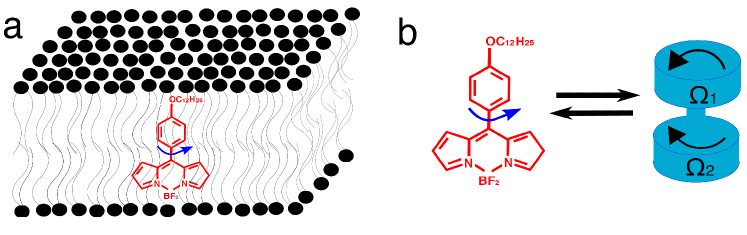
Figure 1: A membrane-bound molecular rotor. (a) A representation of a molecular rotor, in this case a BODIPY rotor, in a biological membrane. (b) Our simplified model of a molecular rotor is composed of two counter-rotating disks, one with angular velocity $\Omega_{1}$ in the upper leaflet, and the second with angular velocity $\Omega_{2}$ in the bottom leaflet.

In order to determine the relaxation time of an excited molecular rotor in a membrane we will make a considerable simplification: we assume the molecular rotor is made of two counter-rotating disks, one in each leaflet (see Fig. 1). As outlined below the effective velocity of two counter-rotating disks can be interpreted as a combination of two axillary problems discussed below: 1) the velocity due to a disk rotating in a viscous 2D flow configuration following the original model of Saffman and Delbrück [11], and 2) the flow due to a disk rotating in a 2D “Brinkman fluid” [12], where there is additional friction on the leaflet, as in the case of a supported bilayer [26, 27, 28].

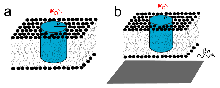
Figure 2: Hydrodynamic characterization. (a) A rotating disk of radius $R$ with angular velocity $\Omega$ in a biological membrane surrounded on both sides by an infinite outer fluid. The leaflets are assumed to have the same properties. (b) A rotating disk of radius $R$ and angular velocity $\Omega$ in a membrane that is in the vicinity of a rigid wall. The fluid dissipates momentum to the wall with a friction coefficient $b_{w}$.

Auxiliary Problems. Consider a disk of radius $R$ rotating with an angular velocity $\Omega$ in a 2D viscous fluid of viscosity $\eta_{m}$. The velocity field $\mathbf{v}$ in the membrane is governed by the Stokes equations, $\eta_{m}\nabla^{2}\mathbf{v}=\nabla p$, where $p$ is the pressure field. Here we have neglected the influence of the surrounding fluid on the membrane ($h\eta/\eta_{m}\ll 1$). From symmetry, we can assume that the flow field is in the $\mathbf{e}_{\theta}$ direction and is a function of $r$ alone, such that $\mathbf{v}=v(r)\mathbf{e}_{\theta}$. For a solution of this form the incompressibility requirement is implicitly satisfied and there are no gradients of pressure. The equation of motion is thus the Laplace equation:

$$\nabla^{2}\mathbf{v}={\bf 0},$$ (2)

which is to be solved with boundary conditions,

$$\mathbf{v}(r=R)=\mathbf{\Omega}\times\mathbf{R}=\Omega R\mathbf{e}_{\theta}\quad\text{and}\quad\mathbf{v}(r\rightarrow\infty)={\bf 0}.$$ (3)

The solution is

$$\mathbf{v}(r)=\frac{\Omega R^{2}}{r}\mathbf{e}_{\theta}.$$ (4)

A straightforward calculation from the surface shear stress, $\sigma_{r\theta}$, integrated over the disk surface, yields the well-known rotational resistance of a cylinder in a 2D membrane [11],

$$\Lambda_{R,\text{I}}=4\pi\eta_{m}R^{2}.$$ (5)

Next consider a disk that is rotating with angular velocity $\Omega$ in a 2D Brinkman fluid, such as for the case of a membrane close to a rigid wall. This flow model introduces an effective force on the membrane due to viscous stresses from the surrounding fluid. We follow Evans and Sackmann [12] in writing the equation of motion,

$$\eta_{m}\nabla^{2}\mathbf{v}-\beta_{w}\mathbf{v}={\bf 0}\quad\text{with}\quad\mathbf{v}=v(r)\mathbf{e}_{\theta},$$ (6)

where $\beta_{w}$ is the friction coefficient with the wall. The boundary conditions are similar to Eq. (3). The solution is

$$\mathbf{v}(r)=\frac{\Omega RK_{1}(\gamma r)}{K_{1}(\gamma R)}\mathbf{e}_{\theta},$$ (7)

where $K_{i}(\cdot)$ is the modified Bessel function of the second kind of order $i$ and $\gamma^{2}=\beta_{w}/\eta_{m}$. The rotational resistance follows as [12]

$$\Lambda_{R,\text{II}}=\left(4\pi\eta_{m}R^{2}\right)\left(1+\frac{\gamma RK_{0}(\gamma R)}{2K_{1}(\gamma R)}\right)=\frac{2\pi\eta_{m}R^{3}\gamma K_{2}(\gamma R)}{K_{1}(\gamma R)}.$$ (8)

Momentum is conserved up to distances $1/\gamma$ and at larger distances is lost due to friction, such that, in the limit $r\ll\gamma^{-1}$, Eq. (7) converges to Eq. (4) and Eq. (8) converges to Eq. (5).

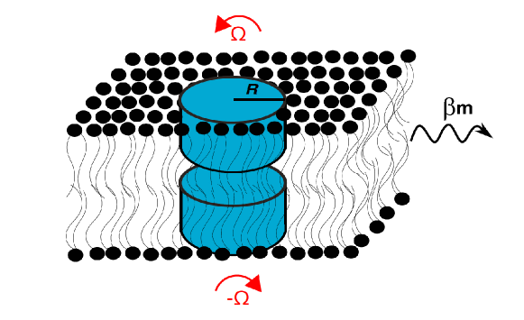
Figure 3: Two counter-rotating disks of radius $R$, respectively with angular velocities $\Omega_{1}$ and $\Omega_{2}$, in a membrane surrounded on both sides by an infinite outer fluid. We denote the friction between the layers of the membrane as $\beta_{m}$.

Two counter-rotating disks in a membrane. Now consider a molecular rotor composed of two connected disks each of radius $R$ immersed between two membrane leaflets. The top disk rotates with angular velocity $\Omega_{1}$ and the bottom disk rotates in the opposite direction with angular velocity $\Omega_{2}$ (see Fig. 3). Suppose that the interleaflet friction is $\beta_{m}$ and as before assume that $\beta_{m}$ and $\eta_{m}$ are large enough to neglect the stress coming from the outer fluid. The equations of motion for such a case can be written as,

$$\eta_{m}\nabla^{2}\mathbf{v_{1}}-\beta_{m}(\mathbf{v_{1}-v_{2}})={\bf 0},$$ (9)

$$\eta_{m}\nabla^{2}\mathbf{v_{2}}-\beta_{m}(\mathbf{v_{2}-v_{1}})={\bf 0},$$

where $v_{1}\;(v_{2})$ is the velocity in the upper (lower) leaflet. The boundary conditions are

$$\mathbf{v_{1}}(R)=\Omega_{1}R\mathbf{e}_{\theta}\quad\text{and}\quad\mathbf{v_{1}}(r\to\infty)={\bf 0},$$ (10)

$$\mathbf{v_{2}}(R)=\Omega_{2}R\mathbf{e}_{\theta}\quad\text{and}\quad\mathbf{v_{2}}(r\to\infty)={\bf 0}.$$

We can add and subtract Eqs. (9) and the boundary conditions in order to obtain expressions for the joint velocity $\mathbf{U}=\mathbf{v_{1}}+\mathbf{v_{2}}=U(r)\mathbf{e}_{\theta}$ and the relative velocity $\mathbf{V}=\mathbf{v_{1}}-\mathbf{v_{2}}=V(r)\mathbf{e}_{\theta}$. The joint velocity is similar to Eq. (4),

$$\mathbf{U}(r)=\frac{(\Omega_{1}+\Omega_{2})R^{2}}{r}\mathbf{e}_{\theta}.$$ (11)

The relative velocity satisfies a governing equation similar to the Brinkman, case Eq. (7), with the solution,

$$\mathbf{V}(r)=(\Omega_{1}-\Omega_{2})R\frac{K_{1}(\kappa r)}{K_{1}(\kappa R)}\mathbf{e}_{\theta},$$ (12)

where $\kappa R$ is a non-dimensional radius defined as $\left(\frac{2\beta_{m}}{\eta_{m}}\right)^{1/2}R$.

If the molecule has an initial twist, then it will relax back to equilibrium. In particular, where there is no net torque acting on the molecule, conservation of angular momentum dictates $\Omega_{1}=-\Omega_{2}=\Omega$, such that $U=0$ and

$$V(r)=\frac{\dot{\theta}RK_{1}(\kappa r)}{K_{1}(\kappa R)},$$ (13)

where we used the fact that the relative angular velocity of the two disks is equal to the time-rate-of-change of the change of twist in the molecule, $2\Omega=\dot{\theta}$. The effective rotational resistance of the molecule can be obtained by computing the ratio of the net hydrodynamic torque to the relative angular velocity $\dot{\theta}$ as,

$$\Lambda_{R}=\left(4\pi\eta_{m}R^{2}\right)\left(1+\frac{\kappa RK_{0}(\kappa R)}{2K_{1}(\kappa R)}\right)=\frac{2\pi\eta_{m}R^{3}\kappa K_{2}(\kappa R)}{K_{1}(\kappa R)}.$$ (14)

In the limit $R\ll\kappa^{-1}$, Eq. (14) converges to Eq. (5).

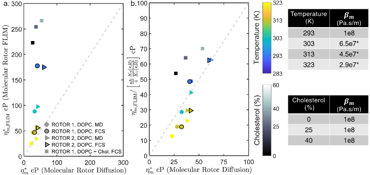
Figure 4: Comparison with experiments. (a) Membrane viscosity evaluated from molecular diffusivity measurements ($\eta_{m}^{*}$) is consistently lower than those obtained from fluorescence lifetime measurements ($\eta^{*}_{m,\rm FLIM}$). Data from DOPC vesicles reported by Dent et al. [17] at different temperatures, and by Wu et al. [15] for different cholesterol concentrations at room temperature. Reported rotor diffusion measurements were obtained via Fluorescence Correlation Spectroscopy (FCS) or Molecular Dynamics (MD). (b) The fold differences between $\eta^{*}_{m,\rm FLIM}$ and $\eta_{m}^{*}$ are in alignment with those expected from Eq. (17). The values of $\beta_{m}$ used for the calculations are shown on the far right. $\beta_{m}$ at 293K was obtained from Ref. [29]. The same value was used at different cholesterol concentrations as $\beta_{m}$ is known to have a weak dependence on cholesterol concentration [23]. As reliable data for $\beta_{m}$ in DOPC vesicles was not available at other temperatures, $\kappa$ was assumed to remain the same across temperature. A * is used to indicate the $\beta_{m}$ satisfying this assumption. This choice is reasonable as $\kappa\propto\sqrt{\beta_{m}/\eta_{m}}$ should only have a weak temperature dependence as both $\beta_{m}$ and $\eta_{m}$ fall with temperature. See SI for additional details.

Fluorescence lifetime of a molecular rotor in a membrane. Following Förster and Hoffmann [18], we neglect inertia of the molecule and express the angular relaxation of the rotor through a spring-dashpot-like response, $\Lambda_{R}\dot{\theta}+k(\theta-\theta_{0})=0$. Here the spring constant $k$ is governed by molecular-scale interactions that drive the molecule back to its equilibrium angular orientation ($\theta_{0}$). The solution yields a classical decaying exponential with a relaxation time constant, $t_{2D}^{*}$, given by

$$t_{2D}^{*}=\frac{\Lambda_{R}}{k}=\frac{2\pi\eta_{m}R^{3}\kappa K_{2}(\kappa R)}{k\,K_{1}(\kappa R)}.$$ (15)

To link the angular relaxation timescale of the rotor to its fluorescence lifetime in the membrane ($\tau_{f,2D}$), we again follow Förster and Hoffmann [18], and assume that the probability of a molecular rotor occupying its excited state is governed by two competing processes: 1) radiative deactivation with a constant lifetime and 2) conformation dependent non-radiative deactivation. Computing the total quantum yield ($\Phi_{f}$) as the time integral of molecular excitation probability yields a relationship linking $\tau_{f,2D}$ and $t_{2D}^{*}$ (see SI),

$$\Phi_{f}=\tau_{f,2D}k_{r}\propto t_{2D}^{*2/3}\propto\Lambda_{R}^{2/3}\propto\eta_{m}^{2/3},$$ (16)

where $k_{r}$ is the radiative decay rate introduced in Eq. (1). Note that Eq. (16) broadly links fluorescence lifetime with the rotor angular relaxation timescale and is also valid in the bulk [18].

Membrane viscosity obtained via Fluorescence Lifetime Imaging Microscopy (FLIM) measurements is consistently larger than those obtained through diffusivity measurements. This fact can be seen in Fig. 4a, where available data in the literature from DOPC vesicles, including results obtained at different temperatures and with varying cholesterol fractions, are plotted to show the systematic overestimation of membrane viscosity by FLIM. The discrepancy can be quantitatively explained solely from differences between rotor hydrodynamics during calibration and during measurements within a membrane.

Molecular rotors are usually calibrated by correlating fluorescence lifetimes measured in the bulk ($\tau_{f,3D}$) with the bulk viscosity ($\eta$) across a series of liquid mixtures [17, 15, 21]. From Eq. (16), it follows that $\tau_{f,3D}\propto t^{*2/3}_{3D}$, the angular relaxation time constant of the rotor in the bulk. Employing the well known rotational resistance of spheres in 3D, $t^{*}_{3D}$ can be shown to be equal to $8\pi\eta R^{3}/k$ (see SI). Comparing $t^{*}_{3D}$ with the result from Eq. (15) that explicitly accounts for the effects of interleaflet friction on rotor hydrodynamics in membranes yields

$$\frac{t_{2D}^{*}}{t_{3D}^{*}}=\frac{\eta_{m}\kappa K_{2}(\kappa R)}{4\eta K_{1}(\kappa R)}=\left(\frac{\tau_{f,2D}}{\tau_{f,3D}}\right)^{3/2}.$$ (17)

In literature, membrane viscosity is usually reported as a thin film viscosity ($\eta_{m}^{*}$) with dimensions of bulk viscosity [17, 15, 21]. $\eta_{m}^{*}$ is related to the 2D membrane viscosity $\eta_{m}$ as $\eta_{m}=\eta_{m}^{*}h$ [12], where $h$ is the thickness of the membrane. Making this substitution in Eq.(17), we see that simply equating fluorescence lifetimes measured on a membrane to those obtained from calibration experiments in the bulk can overestimate membrane thin film viscosity ($\eta_{m}^{*}$) by a factor of $\kappa hK_{2}(\kappa R)/4K_{1}(\kappa R)$.

Rescaling the FLIM membrane viscosity data in Fig. 4a with $\kappa hK_{2}(\kappa R)/4K_{1}(\kappa R)$ leads to a significantly improved agreement between membrane viscosities from the two different measurements (Fig. 4b), where the values of $\beta_{m}$ (for calculating $\kappa$) and $R$ are obtained from the literature (see SI). Physically, the identified factor accounts for two aspects that were previously overlooked. First, the hydrodynamics of molecular rotor relaxation in lipid membranes is affected by the interleaflet friction ($\beta_{m}$) in addition to membrane viscosity. This is accounted for by $\kappa$. Second, the 3D hydrodynamics of molecular rotor relaxation in the bulk (experienced during calibration) is different from the 2D hydrodynamics in a thin lipid bilayer (experienced during measurement). The key variables influencing this discrepancy can be isolated by taking the limit $\kappa\rightarrow 0$ in Eq. (17), whereby the factor simplifies to $h/(2R)$.

These results underscore two key takeaways. Calibration curves obtained via 3D viscosity measurements should be corrected by multiplying the lifetime by a factor of $\left[\kappa hK_{2}(\kappa R)/4K_{1}(\kappa R)\right]^{2/3}$ for directly obtaining the accurate membrane viscosity. Second, if membrane viscosity $\eta_{m}^{*}$ is independently available, e.g., FCS, FRAP or MD simulations, Eq. (17) provides a convenient way to infer interleaflet friction — a hard-to-measure quantity, particularly on curved liposomes and in vivo. In this case, the interleaflet friction can be numerically extracted by solving $\eta^{*}_{m,\rm FLIM}/\eta_{m}^{*}=\kappa hK_{2}(\kappa R)/4K_{1}(\kappa R)$, where $\eta^{*}_{m,\rm FLIM}$ is the uncorrected membrane viscosity (obtained conventionally from bulk viscosity calibrated fluorescence lifetimes). These results also suggest molecular rotors with a larger radius are better suited for measuring interleaflet friction, thus providing guidance on the development of rotors optimized for sensing interleaflet friction (see SI). With further investigation on more molecular rotors and lipid systems, the provided framework can dramatically expand the use of molecular rotors as valuable molecular rheometry probes.

References

- Petty [2013] H. R. Petty, Molecular Biology of Membranes: Structure and Function (Springer Science & Business Media, 2013).
- Singer and Nicolson [1972] S. J. Singer and G. L. Nicolson, Science 175, 720 (1972).
- Henle and Levine [2009] M. L. Henle and A. J. Levine, Physics of Fluids 21 (2009).
- Oppenheimer and Diamant [2009] N. Oppenheimer and H. Diamant, Biophysical Journal 96, 3041 (2009).
- Fitzgerald et al. [2023] J. E. Fitzgerald, R. M. Venable, R. W. Pastor, and E. R. Lyman, Biophysical Journal 122, 1094 (2023).
- Venable et al. [2017] R. M. Venable, H. I. Ingólfsson, M. G. Lerner, B. S. Perrin Jr, B. A. Camley, S. J. Marrink, F. L. Brown, and R. W. Pastor, The Journal of Physical Chemistry B 121, 3443 (2017).
- Shi et al. [2022] W. Shi, M. Moradi, and E. Nazockdast, Physical Review Fluids 7, 084004 (2022).
- Huang et al. [2024] Y. Huang, V. C. Suja, M. Yang, A. V. Malkovskiy, A. Tandon, A. Colom, J. Qin, and G. G. Fuller, Journal of Colloid and Interface Science 653, 1196 (2024).
- Evans and Yeung [1994] E. Evans and A. Yeung, Chemistry and physics of lipids 73, 39 (1994).
- Edidin et al. [1976] M. Edidin, Y. Zagyansky, and T. Lardner, Science 191, 466 (1976).
- Saffman and Delbrück [1975] P. Saffman and M. Delbrück, Proceedings of the National Academy of Sciences 72, 3111 (1975).
- Evans and Sackmann [1988] E. Evans and E. Sackmann, Journal of Fluid Mechanics 194, 553 (1988).
- Haidekker and Theodorakis [2007] M. A. Haidekker and E. A. Theodorakis, Organic & biomolecular chemistry 5, 1669 (2007).
- Nipper et al. [2008] M. E. Nipper, S. Majd, M. Mayer, J. C.-M. Lee, E. A. Theodorakis, and M. A. Haidekker, Biochimica et Biophysica Acta (BBA)-Biomembranes 1778, 1148 (2008).
- Wu et al. [2013] Y. Wu, M. Štefl, A. Olzyńska, M. Hof, G. Yahioglu, P. Yip, D. R. Casey, O. Ces, J. Humpolíčková, and M. K. Kuimova, Physical Chemistry Chemical Physics 15, 14986 (2013).
- López-Duarte et al. [2014] I. López-Duarte, T. T. Vu, M. A. Izquierdo, J. A. Bull, and M. K. Kuimova, Chemical Communications 50, 5282 (2014).
- Dent et al. [2015] M. R. Dent, I. López-Duarte, C. J. Dickson, N. D. Geoghegan, J. M. Cooper, I. R. Gould, R. Krams, J. A. Bull, N. J. Brooks, and M. K. Kuimova, Physical Chemistry Chemical Physics 17, 18393 (2015).
- Förster and Hoffmann [1971] T. Förster and G. Hoffmann, Zeitschrift für Physikalische Chemie 75, 63 (1971).
- Haidekker and Theodorakis [2010] M. A. Haidekker and E. A. Theodorakis, Journal of biological engineering 4, 11 (2010).
- Kuimova [2012] M. K. Kuimova, Physical Chemistry Chemical Physics 14, 12671 (2012).
- Singh et al. [2023] G. Singh, G. George, S. O. Raja, P. Kandaswamy, M. Kumar, S. Thutupalli, S. Laxman, and A. Gulyani, Proceedings of the National Academy of Sciences 120, e2213241120 (2023).
- Adrien et al. [2022] V. Adrien, G. Rayan, K. Astafyeva, I. Broutin, M. Picard, P. Fuchs, W. Urbach, and N. Taulier, Biophysical Chemistry 281, 106732 (2022).
- Anthony et al. [2022] A. A. Anthony, O. Sahin, M. K. Yapici, D. Rogers, and A. R. Honerkamp-Smith, Biophysical Journal 121, 2981 (2022).
- Zgorski et al. [2019] A. Zgorski, R. W. Pastor, and E. Lyman, Journal of chemical theory and computation 15, 6471 (2019).
- Camley and Brown [2013] B. A. Camley and F. L. Brown, Soft Matter 9, 4767 (2013).
- Sackmann [1996] E. Sackmann, Science 271, 43 (1996).
- Stone and Ajdari [1998] H. A. Stone and A. Ajdari, Journal of Fluid Mechanics 369, 151 (1998).
- Oppenheimer and Diamant [2010] N. Oppenheimer and H. Diamant, Physical Review E 82, 041912 (2010).
- Evans and Hochmuth [1976] E. Evans and R. Hochmuth, Biophysical journal 16, 1 (1976).