HRFT: Mining High-Frequency Risk Factor Collections End-to-End via Transformer

Abstract

In quantitative trading, it is common to find patterns in short-term volatile trends of the market. These patterns are known as High-Frequency (HF) risk factors, serving as key indicators of future stock price volatility. Traditionally, these risk factors were generated by financial models relying heavily on domain-specific knowledge manually added rather than extensive market data. Inspired by symbolic regression (SR), which infers mathematical laws from data, we treat the extraction of formulaic risk factors from high-frequency trading (HFT) market data as an SR task. In this paper, we challenge the manual construction of risk factors and propose an end-to-end methodology, Intraday Risk Factor Transformer (IRFT), to directly predict complete formulaic factors, including constants. We use a hybrid symbolic-numeric vocabulary where symbolic tokens represent operators/stock features and numeric tokens represent constants. We train a Transformer model on the HFT dataset to generate complete formulaic HF risk factors without relying on a predefined skeleton of operators (+, $\times$, $/$, $\sqrt{x}$, $\log{x}$, $\cos{x}$). It determines the general shape of the stock volatility law up to a choice of constants, e.g., $f(x)=\tan(ax+b)$ ($x$ is the stock price). We refine the predicted constants (a, b) using the Broyden–Fletcher–Goldfarb–Shanno algorithm (BFGS) to mitigate non-linear issues. Compared to the 10 approaches in SRBench, a living benchmark for SR, IRFT gains a 30% excess investment return on the HS300 and S&P500 datasets, with inference times orders of magnitude faster than theirs in HF risk factor mining tasks.

Introduction

In the past, most research has focused on predicting the expected value of a stock’s future return distribution (Ma, Han, and Wang 2021; Yilmaz and Yildiztepe 2024) by uncovering alphas, also known as return factors (Choi, Jiang, and Zhang 2023). However, high returns often come with high risks. It’s crucial to consider the risk of price volatility to achieve the expected return. (Rezaei, Faaljou, and Mansourfar 2021). A risk factor is a formula that translates historical trading data into a measure of the width of a stock’s future return distribution. As High-Frequency Trading (HFT) markets mature, investors need to respond quickly to short-term market price fluctuations. HFT traders frequently execute orders multiple times during the trading day based on investment managers’ instructions. This paper focuses on capturing short-term volatile trends in HFT markets.

Most risk factor mining relies on experts using financial knowledge to construct models like the Markowitz Mean-Variance Model (Steinbach 2001), CAPM (Merton 1973), and Fama French Models (Taneja 2010; Chiah et al. 2016), then manually selecting the appropriate covariates, also called risk factors. These hand-picked factors often weakly correlate with stock return volatility and lag behind market movements. Statistical models like PCA (Fan, Ke, and Liao 2021; Baek, Cursio, and Cha 2015) and Factor Analysis (Ang, Liu, and Schwarz 2020; Ludvigson and Ng 2007) can obtain latent risk factors but struggle with nonlinear factors. Deep Risk Model (DRM) (Lin et al. 2021) designs risk factors using neural networks to enhance covariance estimation in the Markowitz Mean-Variance Model. However, it focuses on low-frequency risk factors, unsuitable for rapidly changing quantitative trading markets.

Inspired by Symbolic Regression (SR), which infers mathematical patterns from large data sets (Landajuela et al. 2022; Becker et al. 2023), we transform raw historical stock data into indicative volatility signals for quantitative trading. HF risk factor mining tasks are essentially SR tasks. We generate formulaic HF risk factors from raw stock trading features to measure short-term market volatility for the first time. These HF risk factors effectively measure the variance of future stock return distributions. We train a Transformer model from scratch on the HFT dataset instead of fine-tuning an open-source Pre-Trained Model (PTM). Note that most of the capabilities of language models lie in semantic processing. However, the task of generating formulas primarily focuses on tackling numbers and symbols, rather than comprehending extensive vocabularies. So to represent formula factors as sequences, we use direct Polish notation. Operators, variables, and integers are single autonomous tokens. Constants are represented as sequences of 3 tokens: sign, mantissa, and exponent. We preprocess open/close/high/low/volume/vwap features using word expressions. Our embedder and transformer learn from word expressions of stock features as input and formulaic factors as output. The sequence-to-sequence Transformer architecture has 16 attention heads and an embedding dimension of 512, totaling 86M parameters.

The main contributions are summarized as follows:

• We challenge the manual construction of risk factors and propose a data generator for end-to-end HF risk factor mining for downstream tasks and short-term stock market risk measurements.

• To do the HF risk factor mining, we employ a hybrid symbolic-numeric vocabulary where symbolic tokens represent operators$/$stock features and numeric tokens represent constants, then train a Transformer model over the HFT dataset to directly generate full formula factors without relying on skeletons. We refine the prediction constants during the Broyden–Fletcher–Goldfarb–Shanno optimization process (BFGS) as informed guessing, which can alleviate the non-linear issues effectively. Lastly, we utilize generation and inference techniques that enable our model to scale to complex realistic datasets, whereas current works are only suitable for synthetic datasets.

• Our method outperforms the 10 approaches in SRBench in investment simulation experiments over the HS300 and S&P500 dataset, achieving a 30% higher investment return (refer to Fig. 5) and several orders of magnitude faster inference time in factor mining tasks (refer to Fig. 3).

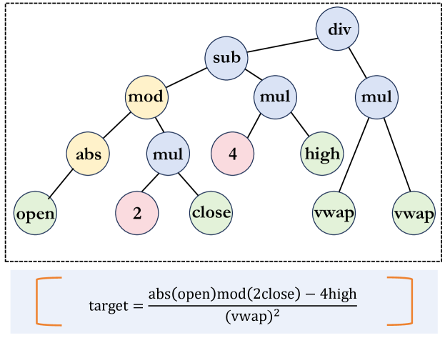
Figure 1: A formulaic HF risk factor can be represented as a binary tree. The nodes are unary operators like ‘mod’ and ‘abs’, and binary operators like ‘sub’, ‘div’, and ‘mul’. The leaves are input features such as ‘high’, ‘open’, ‘close’, and ‘vwap’, along with constants like 2 and 4.

Related Work

Daily Risk Factors. In the past, risk factors were constructed through traditional factor models, often requiring manual screening of covariates. These covariates, such as beta (Prices 1964), size and value (Fama and French 1992), momentum (Carhart 1997), and residual volatility and liquidity (Sheikh 1996), have several shortcomings. Issues include debates over the best covariate sets (Harvey and Liu 2019), weak correlation with equity return volatility (Anatolyev and Mikusheva 2022; Gospodinov, Kan, and Robotti 2019), and factors lagging behind market changes (Li, Li, and Shi 2017). Additionally, statistical models like principal components (Ait-Sahalia and Xiu 2017; De Nard, Ledoit, and Wolf 2021) and factor analysis (Harman 1976) only yield linear risk factors, which are prone to overfitting (Wan et al. 2023). Furthermore, the deep Risk Model (DRM) (Lin et al. 2021), which combines deep learning with the Markowitz mean-variance model, fails when the loss function is non-trivial.

Symbolic Regression. Symbolic Regression (SR) focuses on identifying mathematical expressions that best describe relationships (Biggio et al. 2021; Kamienny et al. 2022). Mining quantitative factors is essentially an SR task, extracting accurate mathematical patterns from historical trading data. The dominant approach is Genetic Programming (GP) (Lin et al. 2019; Zhang et al. 2020; Cui et al. 2021), but it has two drawbacks: slow execution (Langdon 2011), due to the expansive search space requiring numerous generations to converge, and a tendency towards overfitting (Fitzgerald, Azad, and Ryan 2013), dependent on input fitness. Given the time-sensitive nature of quantitative trading, we aim to generate risk factors that effectively capture short-term market volatility.

Language Models. The pre-trained Finbert(Liu et al. 2021) or other pre-trained Fingpt(Yang, Liu, and Wang 2023; Liu, Wang, and Zha 2023; Zhang, Yang, and Liu 2023) mainly focus on semantic processing. However, the task of generating formulaic factors primarily focuses on tackling numbers and symbols, rather than comprehending extensive vocabularies. They encounter difficulties in complex reasoning tasks, like predicting formulas for large numbers(Mishra et al. 2022). In pretraining, models struggle with rarely or never seen symbols. And they can only deal with sequences. We treat HF risk factors as a language for explaining market volatility trends and train a Transformer. This model offers two benefits: They are fast because of leveraging previous experience with inference being a single forward pass. And they are less over fitting-prone, as they do not require loss optimization based on inputs.

Data generation

Instead of using an existing PTM, we provide one. We train a pre-trained language model on HFT datasets. Each training sample $(x,y)\in\mathbb{R}^{W}\times\mathbb{R}$ is input in pairs, aiming to generate an HF risk factor expression $E$ that satisfies $y=E(x)$. For example, we first randomly sample an HF risk factor expression $E$, then sample a set of $M$ input values in $\mathbb{R}^{W}$, $\{x_{k}\mid k\in 1,\ldots,M\}$, and calculate $y_{k}=E(x_{k})$.

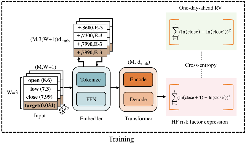
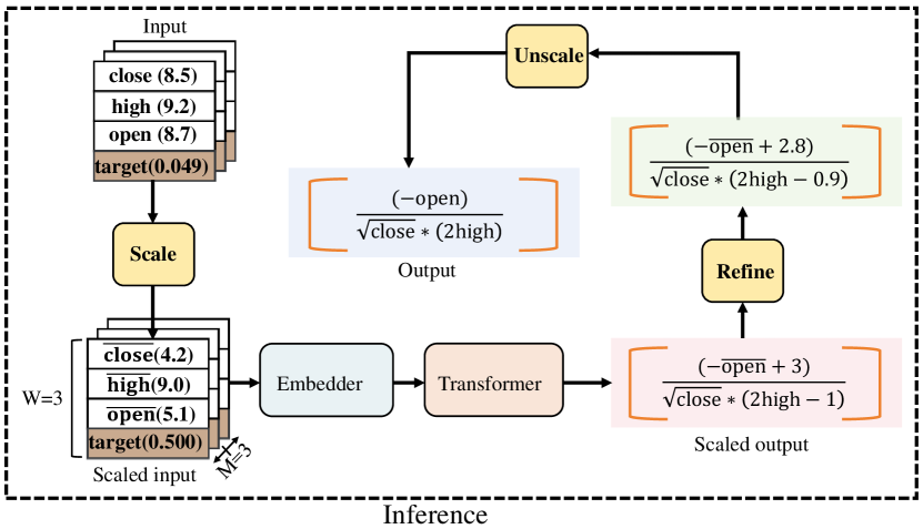
Figure 2: Our risk factor-mining framework operates end-to-end. During training, the Embedder concatenates tokens from three sample pairs into a vector, which is then reduced via a two-layer, ReLU-activated Feed-Forward Network (FFN), producing M embedding vectors for the Transformer. In the inference stage, the complete HF risk factor expression is generated directly. We refine the constants in the factor formulas using the BFGS algorithm and incorporate a scaling process during inference to accommodate diverse HF feature sample points.

Generating functions

Inspired by (Lample and Charton 2019), we randomly generate tree structures composed of mathematical operators, variables, and constants, as shown in Fig. 1.

1. Sample an integer $W$ from $U\{1,W_{\max}\}$, as the expected input dimension of the function $f$.

2. Sample an integer $b$ from $U\{W-1,W+b_{\max}\}$, as the number of binary operators, and then randomly select $b$ binary operators from the set $U\{\text{add},\text{sub},\text{mul},\text{div}\}$. Note that all the binary/unary operators are shown in the sets $O_{b}/O_{u}$. (see Table 4).

3. Construct a binary tree using these $b$ binary operator, drawing on the method of (Lample and Charton 2019).

4. For each leaf node in the tree, randomly select one of the input HF features $x_{w}$, where $w\in 1,\ldots,W$. HFT datasets can be classified into two types: the China and the U.S. stock market.

5. Sample an integer $u$ from $U\{0,u_{\max}\}$, as the number of unary operators, and then randomly select $u$ unary operators from $O_{u}$ in table 4, and insert them randomly into any position in the tree.

6. For each variable $x_{w}$ and the unary operator $u$, apply the random affine transformation, that is, replace $x_{w}$ with $ax_{w}+b$, and replace $u$ with $au+b$, where $(a,b)$ follows the distribution $D_{(a,b)}$.

To independently control the number of unary operators (unrelated to $W$) and binary operators (related to $W$), we cannot directly sample a unary-binary tree as done by (Lample and Charton 2019). We ensure the first $W$ variables are present in the tree, avoiding functions like $x_{2}+x_{4}$ that lack intermediate variables. To enhance expression diversity, we randomly drop out HF variables, allowing our model to set the coefficient of $x_{3}$ to zero. By randomly sampling tree structures and numerical constants, our model rarely encounters identical functions, preventing simple memorization. Detailed parameters for sampling HFT risk factor expressions are in Table 5 (refer to Appendix A for more details).

Generating inputs

Before generating the HF risk factor $E:\mathbb{R}^{W}\to\mathbb{R}$, we first sample $M\in U\{10W,M_{\max}\}$ HF feature values $x_{k}\in\mathbb{R}^{W}$ from the distribution $D_{x}$. Then, we calculate their RV values $y_{k}=E(x_{k})$, and feed them into IRFT. If $x_{k}$ is not in the domain of $E$ or if $y_{k}$ exceeds $10^{100}$, IRFT model will terminate the current generation process and initiate the generation of a new HF risk factor $E$. This approach aims to focus the model’s learning as much as possible on the domain of $E$, providing a simple and effective method. To enhance the diversity of the input distribution during training, we select input samples from a mixture distribution composed of $c$ random centers. The following steps illustrate this process, using distribution $D=2$ as an example (Gaussian or uniform):

1. Randomly sample $c\sim U\{1,c_{\max}\}$ clusters. Each cluster has a weight $w_{i}\sim U(0,1)$, such that $\sum_{i}w_{i}=1$.

2. For each cluster $i\in N_{i}$, randomly draw a centroid $\mu_{i}\sim\mathcal{N}(0,1)^{W}$ from a Gaussian distribution, a variance vector $\sigma_{i}\sim U(0,1)^{W}$ from a uniform distribution, and a distribution type $D_{i}\in\{N,U\}$.

3. For each cluster $i\in N_{i}$, sample $w_{k}M$ input points from $D_{i}(\mu_{i},\sigma_{i})$, and then apply a random rotation using the Haar distribution.

4. Concatenate all the input points and standardize them.

Tokenization

We preprocess HTF stock open/close/high/low/volume/vwap features using word expressions. Our embedder and transformer learn from these feature word expressions as input and formulaic factor word expressions as output. Following (Charton 2021), we represent numbers in decimal scientific notation with four significant digits, using three tokens: sign, mantissa (0 to 9999), and exponent ($E-100$ to $E100$). Referring to (Lample and Charton 2019), we use prefix expressions (Polish notation) for HF risk factors, encoding operators, variables, and integers, and applying the same method for constants. For example, $f(x)=\tan(9.7341x)$ is encoded as $[tan,mul,+,97341,E-3,x]$. The Decoder’s vocabulary includes symbolic tokens (operators and variables) and integer tokens, while the Encoder’s vocabulary only includes integer tokens.

The Method

This section illustrates our IRFT for generating formulaic HF risk factors end-to-end. As shown in Fig. 2, our HF risk factor mining framework consists of two primary stages: Training and Inference.

Model

In this section, we introduce an Embedder to reduce input dimensions, making IRFT more suitable for high-dimensional transaction data. The Transformer model is sensitive to input samples when predicting factor expressions due to the complementarity of the attention heads. Some heads focus on extremes like $-1,0,1$ of exponential functions, while others concentrate on the periodicity of trigonometric functions.

Embedder

Our model is fed with $M$ HFT input points $(x,y)\in\mathbb{R}^{W+1}$, each of which is denoted as $3(W+1)$ tokens of dimension $d_{\text{emb}}$. As $W$ and $M$ increase, it results in long input sequences, e.g. 8400 tokens for $W=6$ and $M=400$, causing computational challenges ($O(n^{2})$) for the Transformer. To alleviate this, we introduce an Encoder to map every input sample to a single embedding. Specifically, this embedder pads the empty input dimensions to $W_{\max}$, then feeds the $3(W_{\max}+1)*d_{\text{emb}}$-dimensional vector into a two-layer feed-forward network (FFN) with ReLU activations to reduce vector’s dimension to $d_{\text{emb}}$. The $M$ embeddings of dimension $d_{\text{emb}}$ are then provided to the Transformer, effectively mitigating computational challenges.

Transformer

We utilize a sequence-to-sequence Transformer model, as proposed by (Vaswani et al. 2017), with 16 attention head and an embedding dimension of 512, totaling 84 million parameters. Following (Charton 2021), we observe that the solution to the factor mining task is an asymmetric model structure with a deeper decoder. In more details, we use 4 layers in the encoder and 16 layers in the decoder. The encoder effectively captures the distinctive features of HFT stock data, such as periodicity and continuity, by mixing short-ranged attention heads focusing on local features with long-ranged attention heads capturing the global form of the HF risk factor. Unlike previous risk factor mining models (Harman 1976; Lin et al. 2021), our model accounts for the periodicity of stock sample points, capturing short-term volatility and cycling in the HFT stock market.

Training.

We employ the Adam optimizer to minimize the cross-entropy loss. Actually, our cross entropy loss calculates the probability distribution of target tokens and risk factor tokens, in order to find the factor token with the maximum probability of the target token. The learning rate is initially set to $2\times 10^{-7}$ and is linearly increased to $2\times 10^{-3}$ over the first 10,000 steps. Following the approach proposed by (Vaswani et al. 2017), we then decay the learning rate as the inverse square root of the step numbers. To assess the model’s performance, We take 10% samples from the same generator as a validation set and trained IRFT model until the accuracy on the validation set was satisfied. We esitimate this process to span approximately 50 epochs, with each epoch consisting of 3 million sample points. Moreover, to minimize the padding waste, we put together sample point with similar lengths, which can ensure ensure more than 3M samples in each batch.

Inference Tricks

We describe four tricks to enhance IRFT’s inference performance. Previous SR models, like (Biggio et al. 2021; Valipour et al. 2021), use a standard skeleton approach, predicting equation skeletons first and then fitting constants. These methods are less accurate and handle limited input dimensions ($W<3$). Our end-to-end (E2E) method predicts functions and constants simultaneously, allowing our model to process more input features ($W=7$) and handle large real-world datasets (about 26M samples).

Refinement

As suggested by (Kamienny et al. 2022), we significantly enhance effectiveness by adding a refinement step: fine-tuning constants using BFGS with our model predictions as initial values. This improves the skeleton method in two ways: providing stronger supervision signals by predicting complete HF risk factor expressions and enhancing constant accuracy with the BFGS algorithm, thereby boosting overall model performance.

Scaling

At the inference stage, we introduce a scaling procedure to ensure accurate predictive factor formulas from samples with varying means and variances. During training, we scale all HF input points to center their distributions at the origin with a variance of 1. For example, let $E$ be the inferred risk factor, $x$ be the input, $\mu=\text{mean}(x)$, and $\sigma=\text{std}(x)$. Then we replace $x$ with $\bar{x}=(x-\mu)/\sigma$, and the model predicts $\hat{E}(\bar{x})=\hat{E}(\sigma x+\mu)$. This allows us to recover an approximate $E$ by unscaling the variables in $\hat{E}$. This approach makes IRFT insensitive to the scale of input points and represents constants outside $D_{(a,b)}$ as multiplications of constants within $D_{(a,b)}$. Unlike our method, DL-based approaches like (Petersen et al. 2019) often fail when samples fall outside the expected value range.

Bagging and decoding

With over 400 sample points, our experiment is less effective. To fully utilize extensive HFT data, we adopt bagging: if HFT input points $M$ exceed 400 during inference, we split the dataset into $B$ bags of 400 stock points each. We then generate $K$ formulaic factor candidates per bag, resulting in $BK$ candidates. Unlike previous language models, our approach generates multiple expressions for each bag.

Inference time

The speedup of our model inference comes from refining HF risk factor expression candidates. Given the large $BC$, we rank candidates by their error on input samples, remove duplicates or redundant factors, and keep the top $C$ candidates for refinement. To accelerate this process, we optimize using a subset of up to 1024 input samples. Parameters $B$, $K$, and $C$ can be fine-tuned for better speed and accuracy. In our experiment, we used $B=100$, $K=10$, $C=10$.

EVALUATION

In this section, we mainly answer the questions below: Q1: How does our proposed framework compare with other state-of-the-art methods based on SR tasks for generating HF risk factor expressions? Q2: How does our model perform as the size of HF risk factor collections increases? Q3: How does our framework perform in more realistic trading settings?

Experimental Settings

Datasets

Our experiments are conducted on HFT data from the U.S. and China stock market (see Table 1). The stock data was obtained from wind. Specifically, we analyze the $W$-dimensional trading data $X\in\mathbb{R}^{W}$ of the 1-min trading level of constituent stocks of the HS300 index and the S&P500 index. We preprocess raw stock open/close/high/low/volume/vwap features using word expressions. It’s important to highlight that our method employs an ascending variable sampling approach for features. This implies that instances such as $x_{2}+x_{3}$ will not occur, but rather samples like $x_{1}+x_{2}+x_{3}$ will be generated. However, we have the flexibility to set the weight in front of $x_{1}$ to zero. The target value is the one-day-ahead RV, defined as $RV(t,j;n)=\sum_{j=1}^{n}(\ln P_{t,j}-\ln P_{t,j-1})^{2}$, where $n$ is the number of intraday trading intervals and $P_{i,j}$ is the closing price of the $j$-th interval of the $i$-th trading day (Andersen and Bollerslev 1998).

Table 1: Market Data Overview

	The U.S. Market	The China Market
Training	2023/01/03-2023/10/31	2022/10/31-2023/08/31
Evaluate	2023/10/31-2023/12/29	2023/08/31-2023/10/31
Sample Size	18,330,000	7,964,160

Compared Approaches

We compare IRFT with advanced methods from SRBench(La Cava et al. 2021) in generating HF risk factor expressions.

• DL-based methods: DSR(Petersen et al. 2019) employs a parameterized neural network to model the distribution of a mathematical expression, represented as a sequence of operators and variables in the corresponding expression tree.

• GP-based method: GPLEARN is a evolutionary algorithm specialized in SR, where the mathematical expressions of a population ‘evolve’ through the use of genetic operators such as mutation, crossover, and selection. GENEPRO is another GP framework capable of handling not only regression feature variables but also environmental observations related to reinforcement learning (though we do not consider this option here).

• ML-based methods: To evaluate the model more comprehensively, we compare IRFT with the end-to-end ML methods in SRBench. These methods take a week’s HF stock features as input and predict one-day-ahead RV. AdaBoost ensembles decision trees to directly predict stock trends. Lasso Lars is a linear regression method that combines Lasso and LARS. Random Forest is an ensemble learning method that averages the regression results from multiple decision trees. The other ML methods are SGD Regressor (Bottou 2010), MLP and Linear Regression. These ML models do not generate formulaic HF risk factor expressions, but only output volatility prediction values. The hyperparameters are set by SRBench.

Evaluation Metrics

Each of the following four positive indicators assesses the correlation between actual stock price volatility and future volatility forecasts.

$\boldsymbol{R^{2}.}$

It measures the explanatory degree of one-day-ahead RV variation for factor-mining tasks.

$$R^{2}=1-\frac{\sum_{i=1}^{M_{\text{test}}}(y_{i}-\hat{y}_{i})^{2}}{\sum_{i=1}^{M_{\text{test}}}(y_{i}-\bar{y})^{2}}$$ (1)

$\boldsymbol{IC^{*}.}$

It is the cross-section correlation coefficient of the HF risk factor values and the one-day-ahead RV values of trading stocks, which ranges from $[-1,1]$.

$$IC^{*}=\bar{\sigma}\left(\sum_{i=1}^{k}w_{i}f_{i}(X),y_{i}\right)$$ (2)

Where, $\sigma(f_{l}(X),f_{k}(X))=\frac{\sum_{l=1}^{n}(f_{tl}-\bar{f}_{t})(f_{tk}-\bar{f}_{t})}{\sqrt{\sum_{l=1}^{n}(f_{tl}-\bar{f}_{t})^{2}\sum_{k=1}^{n}(f_{tk}-\bar{f}_{t})^{2}}}$, $y_{i}$ is the one-day-ahead RV. We simplify the calculation by taking the daily average of the Pearson correlation coefficient between the HF risk factors and the targets over all trading days. $\bar{\sigma}\left(\sum_{i=1}^{k}w_{i}f_{i}(X),y_{i}\right)=E_{t}\left[\sigma\left(\sum_{i=1}^{k}w_{i}f_{i}(X),y_{i}\right)\right]$ and $\bar{\sigma}\left(\sum_{i=1}^{k}w_{i}f_{i}(X),y_{i}\right)\in[-1,1]$.

$\boldsymbol{RankIC^{*}.}$

It is $IC^{*}$ ranking of the HF risk factor values and the one-day-ahead RV of the selected stocks.

$$RankIC^{*}=\bar{\sigma}\left(r\left(\sum_{i=1}^{k}w_{i}f_{i}(X)\right),r(y_{i})\right)$$ (3)

Where, $r(\cdot)$ is the ranking operator of the HF risk factor value and the one-day-ahead RV.

$\boldsymbol{IR^{*}.}$

It is the mean of the $IC^{*}$ divided by the standard deviation of these $IC^{*}$.

$$IR^{*}=\frac{\bar{Ret}_{t}^{IC}}{\text{std}(Ret_{t}^{IC})}$$ (4)

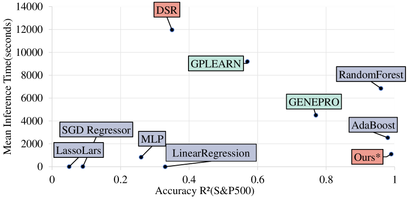
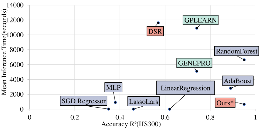
Figure 3: The Pareto plot compares our framework with baselines like DL-based methods, ML-based methods, and GP-based methods from SRBench about the average inference time and test performance.

Table 2: Main results of S&P500 Index and HS300 Index. Values after ”$\pm$” represents the standard deviation, and the rest are the mean values, while the rest are mean values. “↑” indicates that higher values are better.

Method	S&P 500			HS 300
	$IC^{*}$ (↑)	Rank $IC^{*}$ (↑)	$IR^{*}$ (↑)	$IC^{*}$ (↑)	Rank $IC^{*}$ (↑)	$IR^{*}$ (↑)
DSR	$0.0437\pm 0.0054$	$0.0453\pm 0.0071$	$0.2506\pm 0.0246$	$0.0427\pm 0.0088$	$0.0456\pm 0.0059$	$0.3395\pm 0.0637$
GPLEARN	$0.0250\pm 0.0099$	$0.0547\pm 0.0073$	$0.4876\pm 0.0307$	$0.0494\pm 0.0062$	$0.0480\pm 0.0063$	$0.3600\pm 0.0368$
GENEPRO	$0.0470\pm 0.0068$	$0.0550\pm 0.0163$	$0.2098\pm 0.0339$	$0.0444\pm 0.0049$	$0.0528\pm 0.0090$	$0.4787\pm 0.0453$
Ours*	$\textbf{0.0662}\pm 0.0077$	$\textbf{0.0720}\pm 0.0085$	$\textbf{0.4960}\pm 0.0817$	$\textbf{0.0618}\pm 0.0083$	$\textbf{0.0683}\pm 0.0088$	$\textbf{0.6460}\pm 0.1002$

Table 3: Top 5 HF risk factor expressions based on $IC^{*}$ values in the HF risk factor collections (S&P500 Index).

No.	HF risk factor	$IC^{*}$
1	$0.6*\log((2709.5-0.9\cdot\sin(0.4\cdot\text{close}-2.0)+16.7-40.1/((0.2\cdot\text{low}+0.4))))-0.4)+0.2$	0.0820
2	$-8.4+8.2/(-0.7*(-0.1-0.1/(1.9-0.5\cdot\text{close})))$	0.0641
3	$2.8*\sqrt{0.1/((-0.2\cdot\text{open}-11.7*(13.7-2.6\cdot\text{open})+1.0)^{2})}-1.0$	0.0635
4	$1.3*(0.2*\lvert-0.1\cdot\text{low}+5.1\rvert+0.2)+1.3$	0.0558
5	$0.8/((-0.1\cdot\text{open}-(0.1\cdot\text{high}+3.6)*(-3.0*(5.2-1.5\cdot\text{volume})*(40.0-7.0\cdot\text{low})+2046.9)))-0.5$	0.0522

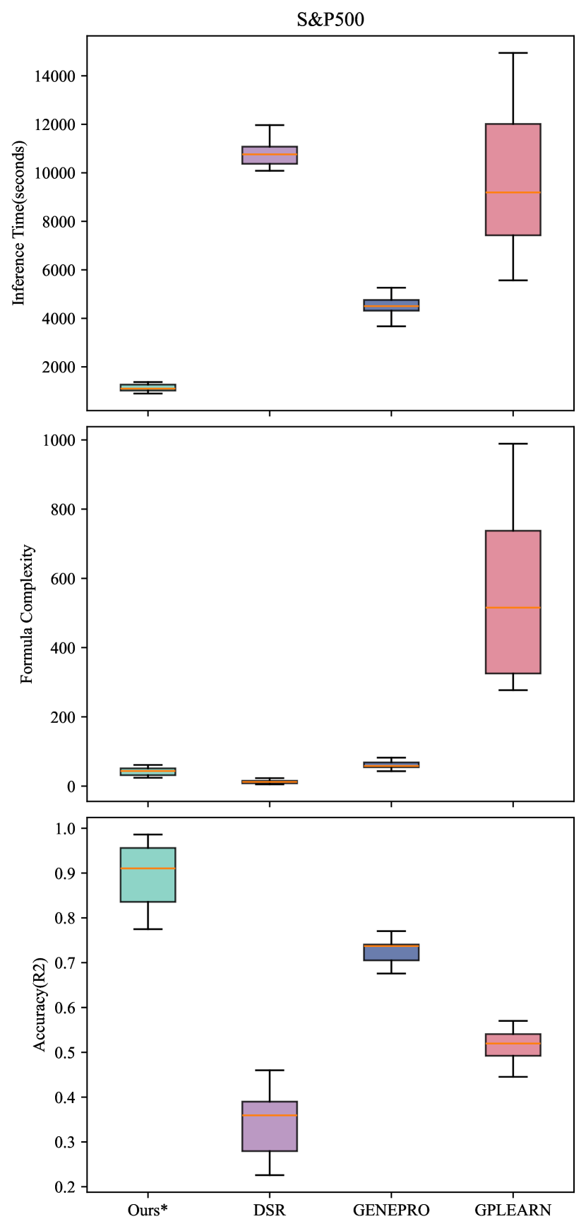
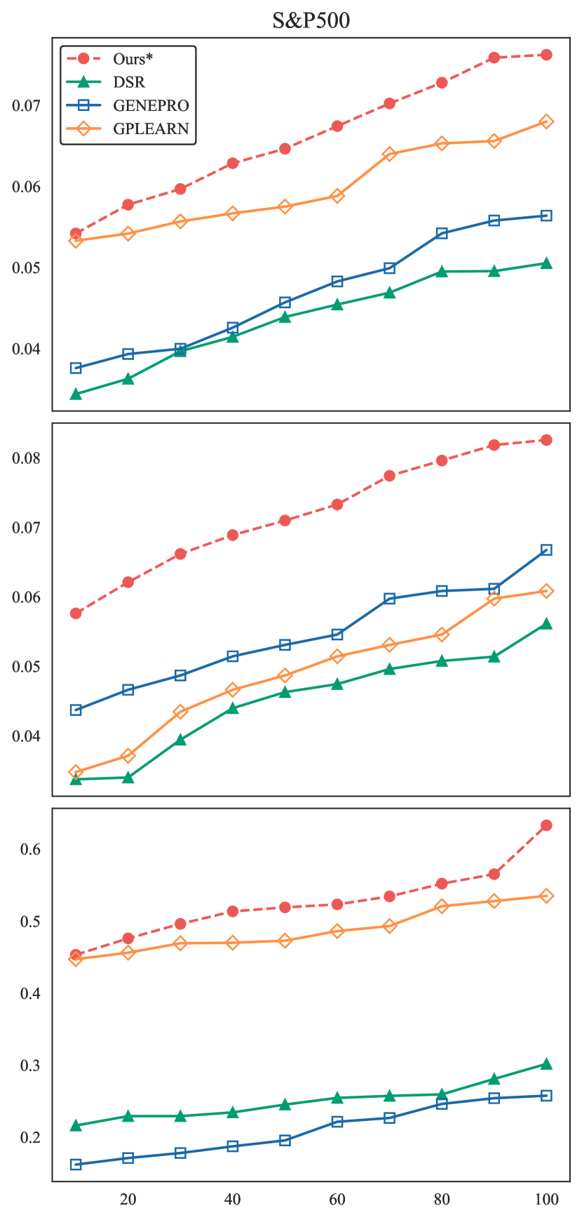
Figure 4: (a) Performance of different methods on S&P500 Index (U.S. market). (b) A comparison of different factor generation methods using $IC^{*}$, $RankIC^{*}$ and $IR^{*}$ for various factor pool sizes.

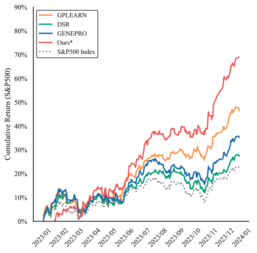
Figure 5: (a) The correlation of the HF risk factor collections on S&P500 Index. (b) Portfolio simulations on the S&P500 Index: a backtesting comparison.

Comparison across all HF risk factor generators (RQ1)

We evaluate the performance of three baseline methods on HFT data sets derived from the constituents of the S&P500 index. The results, in terms of inference time, expression complexity, and prediction performance ($R^{2}$), are presented using box plots in Fig. 4.

Our method demonstrates a significant advantage in inference time, being 17 times faster than DSR, and exhibits a narrow distribution, indicating high stability and efficiency. This is attributed to our method’s use of the efficient encoding and decoding mechanism, which transforms the features and target variables in the data sets into the input and output of HF risk factor expression tokens, thereby reducing the search space and computation of the symbolic solver. GPLEARN, while faster than DSR, has a more dispersed distribution, suggesting its performance is more sensitive to the data sets. This could be due to GPLEARN’s use of genetic programming to search for symbolic expressions, which often results in overly long and complex expressions and lacks effective regularization mechanisms. In terms of expression complexity, DSR generates the most concise expressions, possibly due to its use of a regularization term to penalize excessively long and complex expressions, thus avoiding overfitting and redundancy. Our method and DSR have similar expression complexity, which is significantly lower than GPLEARN. GPLEARN generates the longest expressions, with an average length of 512 and a maximum length of 989. Regarding prediction performance, our method generates HF risk factor expressions with an $R^{2}$ value of 0.92, significantly outperforming other methods. This suggests that our method can accurately fit and predict the volatility trend of the stock data sets. GPLEARN and GENEPRO are the second best methods, with comparable $R^{2}$ values. Moreover, DSR performs the worst, with a low and large $R^{2}$ variation, ranging from 0.23 to 0.46. Moreover, Fig. 3 demonstrates that our framework surpasses other 10 baselines in SRBench with the highest performance and shortest inference time. .

Table 2 shows that, compared to other baseline methods, our method generates HF risk factors with the highest values of $IC^{*}$, $RankIC^{*}$, and $IR^{*}$, which assess the predictive ability of the generated HF risk factor expressions, like their ability to capture the future stock volatility trend. For the indicators $IC^{*}$ and $RankIC^{*}$ , DSR and GENEPRO perform similarly on both the S&P500 and HS300 index data sets. For the indicator $IR^{*}$, the GP methods based on SR tasks significantly outperform DSR.

Comparison of formulaic generators with varying pool capacity (RQ2)

Fig. 4 presents the mean values of $IC^{*}$, $RankIC^{*}$, and $IR^{*}$ for the HF risk factor collections generated by different methods under varying factor pool sizes. From this figure, our framework, IRFT, consistently exhibits the highest $IC^{*}$, $RankIC^{*}$ and $IR^{*}$ values across all factor pool sizes. Furthermore, IRFT demonstrates scalability with respect to the factor pool size. That is, as the factor pool size increases, it continues to identify superior HF risk factor expressions without succumbing to overfitting or redundancy issues. This suggests that IRFT can effectively leverage the semantic information of the large language model, as well as the flexibility of symbolic regression, to generate diverse and innovative HF risk factors.

Investment Simulation (RQ3)

During backtesting period, we analyze factor set heat maps (Figures 5(a) and 7(a)) and select 10 independent risk factors(the more information they contain). We calculate risk factor scores for all assets in the portfolio ($k=30$ stocks in our paper) for each adjustment period (each trading day). The factor score for the $s$th stock is $a(s)=\sum_{n=1}^{N}w(n)V(s,n)$, where $w(n)$ is the weight of the $n$th factor ($\text{IC}^{*}$ value) and $V(s,n)$ is the $n$th factor value of the $s$th stock. These factors help select high-yielding stocks for the portfolio. As shown in Figure 5(b), we record cumulative net returns over a one-year test period. Despite the fact that our framework does not explicitly optimize for absolute return, it still performs well in the backtest, even during the test period when the international environment is unstable and the domestic economy slows down. Compared with other methods, our framework can still achieve the highest profit, exceeding the second-place method GENEPRO by 21%. Table 3 presents the top five HF risk factors selected from the HF risk factor collections, based on their $IC^{*}$ values. These factors, which include arbitrary constant terms, are highly flexible and can be adapted to any range of values. For simplicity, we round the constant terms to one decimal place.

Conclusion

In this paper, we introduce a transformer model for HF risk factor mining, replacing traditional manual factor construction. Unlike previous language models that focus on word relationships for natural language comprehension, our model uses a hybrid symbolic-numeric vocabulary. Symbolic tokens represent operators/stock features, while numeric tokens denote constants. The Transformer predicts complete formulaic factors end-to-end and refines constants using a non-convex optimizer. Our framework outperforms 10 approaches in SRBench and scales to a 6-dimensional, 26 million HF dataset. Extensive experiments show that IRFT surpasses formulaic risk factor mining baselines, achieving a 30% excess investment return on HS300 and S&P500 datasets and significantly speeding up inference times.

Appendix A Appendix

Table 4: List of all operators employed within our framework.

Category	Operator	Description
CS-B	add(x,y)	Arithmetic operators
	sub(x,y)
	mul(x,y)
	div(x,y)
CS-U	inv(x)	The inverse of x
	sqr(x)	The square of x
	sqrt(x)	The square root of x
	sin(x)	The sine of x
	cos(x)	The cosine of x
	tan(x)	The tangent of x
	atan(x)	The arctangent of x
	log(x)	The logarithm of x
	exp(x)	The exponential value of x
	abs(x)	The absolute value of x

Table 5: Detailed parameter settings of IRFT.

Parameter	Description	Value
		W=5(S&P500)	W=5(SSE50)
W_max	Max input dimension	10
D_((a,b))	Distribution of (a, b) in an affine transformation	sign U-1,1, mantissa U(0,1), exponent U(-2,2)
b_max	Max binary operators	5+W	5+W
O_b	Binary operators	add,sub,mul,div
u_max	Max unary operators	5	5
O_u	Unary operators	inv,abs,sqr,sqrt,sin,cos,tan,atan,log,exp
M_min	Min number of points	10D
M_max	Max number of points	200
c_max	Max number of candidate function clusters	10

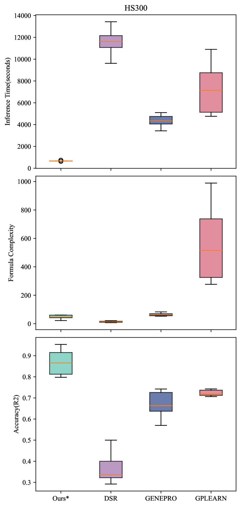
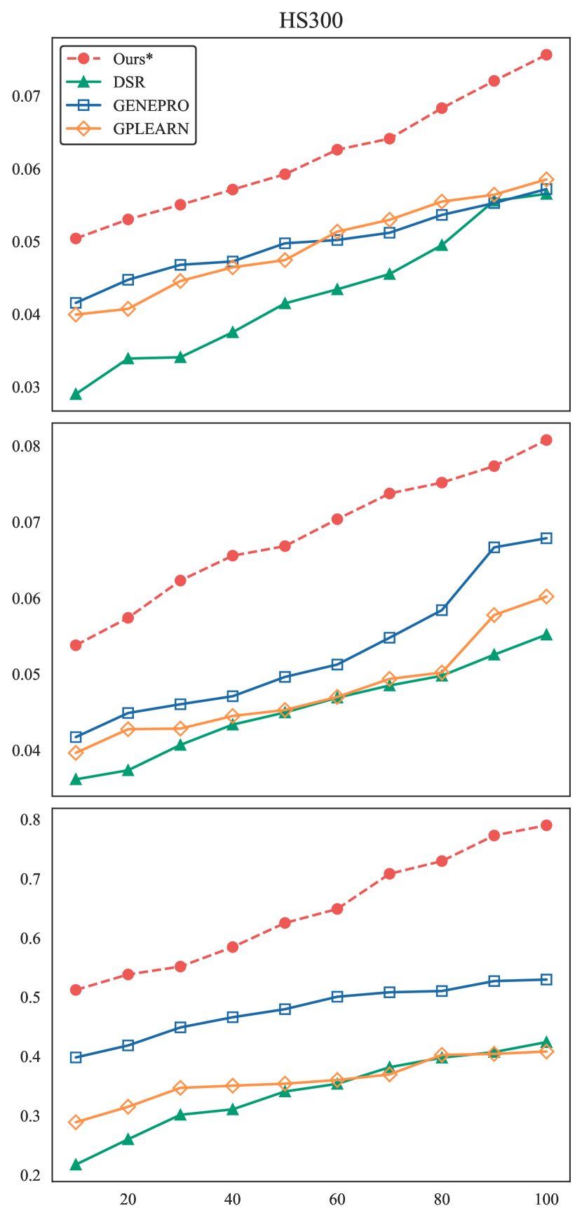
Figure 6: (a) Performance of different methods on HS300 Index(the China market). (b) A comparison of different factor generation methods using $IC^{*}$ , $RankIC^{*}$ and $IR^{*}$ for various factor pool sizes.

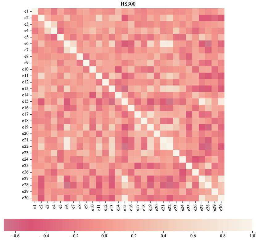
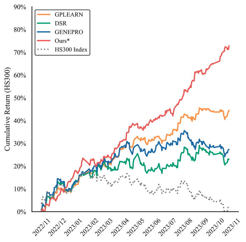
Figure 7: (a) The correlation of the HF risk factor collections on HS300 Index. (b) Portfolio simulations on the HS 300 Index: a backtesting comparison.

Collection of operators

Table 4 lists the unary and binary operators used in this paper. We use these binary operators and 10 unary operators to generate HF risk factor expressions. It should be noted that these operators are based on cross-section, not on time series. Since this paper considers two input options for HFT market data sets of different countries, one of which contains time series features reflecting different time windows, we do not discuss the operators at the time-series level.

The detailed parameter set description

Table 5 shows the detailed parameter settings of our data generator when using the IRFT model to sample HF risk factor expressions on two types of HFT data sets in the China and the U.S. stock market. Among them, $W_{\max}$ represents the maximum feature dimension of the input data set allowed by our model, which is 10. $M_{\min}/M_{\max}$ represents the minimum/maximum value of the logarithm of the sample pairs contained in a data packet $B$. $b_{\max}/u_{\max}$ represents the number of binary/unary operators sampled. $O_{b}/O_{u}$ represents the set of binary/unary operators sampled. $D_{(a,b)}$ represents the coefficient distribution of random affine transformation for each variable $x_{w}$ and unary operator $u$, that is, replacing $x$ with $ax_{w}+b$, replacing $u$ with $au+b$; $c_{\max}$ is the number of candidate functions in the refine stage.

Performance of different methods under the China HFT market

As depicted in Fig. 6, our method demonstrates a significant advantage in terms of inference time, outperforming the slowest method, DSR six times. The concentrated distribution of inference times indicates high stability and efficiency of our method. GPLEARN, while faster than DSR, exhibit more dispersed distributions, suggesting their performance is more susceptible to variations in the stock data set. In terms of expression complexity, DSR generates the most concise expressions, suggesting its ability to find simple and effective HF risk factor expressions. Regarding prediction performance, our method generates HF risk factor expressions with a value of $R^{2}$ of 0.87, significantly outperforming other methods. The next best method is GPLEARN, followed by GENEPRO, with DSR performing the worst.

Comparison of formulaic generators with varying pool capacity(HS300 Index).

We further extend our analysis to evaluate the performance of different methods in generating HF risk factor collections for the China stock market. As depicted in Fig. 6, our method, IRFT, consistently exhibits the highest values of $IC^{*}$, $RankIC^{*}$, and $IR^{*}$ across all factor pool sizes. This indicates its superior predictive ability in generating HF risk factors. The performance of the other three methods does not differ significantly.

HF risk collections for investment simulation(SSE50 Index).

As depicted in Fig. 7(a), we have implemented a filtering process to delete HF risk factors with high correlation. Consequently, the HF risk factor collection retains 10 unique HF risk factors. As illustrated in Fig. 7(b), we recorded the cumulative net value of all strategies over a one-year test period in the China HFT market. Our framework outperforms other methods, achieving the highest profit and exceeding other SR methods by 30%. Next, GPLEARN obtains higher portfolio returns than the remaining two benchmarks. The one that receive the lowest return is DSR. The backtest results demonstrate that our method still has maintained stable growth throughout the backtest period.

References

- Ait-Sahalia and Xiu (2017) Ait-Sahalia, Y.; and Xiu, D. 2017. Using principal component analysis to estimate a high dimensional factor model with high-frequency data. Journal of Econometrics, 201(2): 384–399.
- Anatolyev and Mikusheva (2022) Anatolyev, S.; and Mikusheva, A. 2022. Factor models with many assets: strong factors, weak factors, and the two-pass procedure. Journal of Econometrics, 229(1): 103–126.
- Andersen and Bollerslev (1998) Andersen, T. G.; and Bollerslev, T. 1998. Answering the skeptics: Yes, standard volatility models do provide accurate forecasts. International economic review, 885–905.
- Ang, Liu, and Schwarz (2020) Ang, A.; Liu, J.; and Schwarz, K. 2020. Using stocks or portfolios in tests of factor models. Journal of Financial and Quantitative Analysis, 55(3): 709–750.
- Baek, Cursio, and Cha (2015) Baek, S.; Cursio, J. D.; and Cha, S. Y. 2015. Nonparametric factor analytic risk measurement in common stocks in financial firms: Evidence from Korean firms. Asia-Pacific Journal of Financial Studies, 44(4): 497–536.
- Becker et al. (2023) Becker, S.; Klein, M.; Neitz, A.; Parascandolo, G.; and Kilbertus, N. 2023. Predicting ordinary differential equations with transformers. In International Conference on Machine Learning, 1978–2002. PMLR.
- Biggio et al. (2021) Biggio, L.; Bendinelli, T.; Neitz, A.; Lucchi, A.; and Parascandolo, G. 2021. Neural symbolic regression that scales. In International Conference on Machine Learning, 936–945. PMLR.
- Bottou (2010) Bottou, L. 2010. Large-scale machine learning with stochastic gradient descent. In Proceedings of COMPSTAT’2010: 19th International Conference on Computational StatisticsParis France, August 22-27, 2010 Keynote, Invited and Contributed Papers, 177–186. Springer.
- Carhart (1997) Carhart, M. M. 1997. On persistence in mutual fund performance. The Journal of finance, 52(1): 57–82.
- Charton (2021) Charton, F. 2021. Linear algebra with transformers. arXiv preprint arXiv:2112.01898.
- Chiah et al. (2016) Chiah, M.; Chai, D.; Zhong, A.; and Li, S. 2016. A Better Model? An empirical investigation of the Fama–French five-factor model in Australia. International Review of Finance, 16(4): 595–638.
- Choi, Jiang, and Zhang (2023) Choi, D.; Jiang, W.; and Zhang, C. 2023. Alpha go everywhere: Machine learning and international stock returns. Available at SSRN 3489679.
- Cui et al. (2021) Cui, C.; Wang, W.; Zhang, M.; Chen, G.; Luo, Z.; and Ooi, B. C. 2021. AlphaEvolve: A Learning Framework to Discover Novel Alphas in Quantitative Investment. In Proceedings of the 2021 International Conference on Management of Data, 2208–2216.
- De Nard, Ledoit, and Wolf (2021) De Nard, G.; Ledoit, O.; and Wolf, M. 2021. Factor models for portfolio selection in large dimensions: The good, the better and the ugly. Journal of Financial Econometrics, 19(2): 236–257.
- Fama and French (1992) Fama, E. F.; and French, K. R. 1992. The cross-section of expected stock returns. the Journal of Finance, 47(2): 427–465.
- Fan, Ke, and Liao (2021) Fan, J.; Ke, Y.; and Liao, Y. 2021. Augmented factor models with applications to validating market risk factors and forecasting bond risk premia. Journal of Econometrics, 222(1): 269–294.
- Fitzgerald, Azad, and Ryan (2013) Fitzgerald, J.; Azad, R. M. A.; and Ryan, C. 2013. A bootstrapping approach to reduce over-fitting in genetic programming. In Proceedings of the 15th annual conference companion on Genetic and evolutionary computation, 1113–1120.
- Gospodinov, Kan, and Robotti (2019) Gospodinov, N.; Kan, R.; and Robotti, C. 2019. Too good to be true? Fallacies in evaluating risk factor models. Journal of Financial Economics, 132(2): 451–471.
- Harman (1976) Harman, H. H. 1976. Modern factor analysis. University of Chicago press.
- Harvey and Liu (2019) Harvey, C. R.; and Liu, Y. 2019. A census of the factor zoo. Available at SSRN 3341728.
- Kamienny et al. (2022) Kamienny, P.-A.; d’Ascoli, S.; Lample, G.; and Charton, F. 2022. End-to-end symbolic regression with transformers. Advances in Neural Information Processing Systems, 35: 10269–10281.
- La Cava et al. (2021) La Cava, W.; Orzechowski, P.; Burlacu, B.; de França, F. O.; Virgolin, M.; Jin, Y.; Kommenda, M.; and Moore, J. H. 2021. Contemporary symbolic regression methods and their relative performance. arXiv preprint arXiv:2107.14351.
- Lample and Charton (2019) Lample, G.; and Charton, F. 2019. Deep learning for symbolic mathematics. arXiv preprint arXiv:1912.01412.
- Landajuela et al. (2022) Landajuela, M.; Lee, C. S.; Yang, J.; Glatt, R.; Santiago, C. P.; Aravena, I.; Mundhenk, T.; Mulcahy, G.; and Petersen, B. K. 2022. A unified framework for deep symbolic regression. Advances in Neural Information Processing Systems, 35: 33985–33998.
- Langdon (2011) Langdon, W. B. 2011. Graphics processing units and genetic programming: an overview. Soft computing, 15: 1657–1669.
- Li, Li, and Shi (2017) Li, H.; Li, Q.; and Shi, Y. 2017. Determining the number of factors when the number of factors can increase with sample size. Journal of Econometrics, 197(1): 76–86.
- Lin et al. (2021) Lin, H.; Zhou, D.; Liu, W.; and Bian, J. 2021. Deep risk model: a deep learning solution for mining latent risk factors to improve covariance matrix estimation. In Proceedings of the Second ACM International Conference on AI in Finance, 1–8.
- Lin et al. (2019) Lin, X.; Chen, Y.; Li, Z.; and He, K. 2019. Revisiting Stock Alpha Mining Based On Genetic Algorithm. Technical report, Technical Report. Huatai Securities Research Center. https://crm. htsc. com ….
- Liu, Wang, and Zha (2023) Liu, X.-Y.; Wang, G.; and Zha, D. 2023. Fingpt: Democratizing internet-scale data for financial large language models. @articlezhang2023instruct, title=Instruct-fingpt: Financial sentiment analysis by instruction tuning of general-purpose large language models, author=Zhang, Boyu and Yang, Hongyang and Liu, Xiao-Yang, journal=arXiv preprint arXiv:2306.12659, year=2023 arXiv preprint arXiv:2307.10485.
- Liu et al. (2021) Liu, Z.; Huang, D.; Huang, K.; Li, Z.; and Zhao, J. 2021. Finbert: A pre-trained financial language representation model for financial text mining. In Proceedings of the twenty-ninth international conference on international joint conferences on artificial intelligence, 4513–4519.
- Ludvigson and Ng (2007) Ludvigson, S. C.; and Ng, S. 2007. The empirical risk–return relation: A factor analysis approach. Journal of financial economics, 83(1): 171–222.
- Ma, Han, and Wang (2021) Ma, Y.; Han, R.; and Wang, W. 2021. Portfolio optimization with return prediction using deep learning and machine learning. Expert Systems with Applications, 165: 113973.
- Merton (1973) Merton, R. C. 1973. An intertemporal capital asset pricing model. Econometrica: Journal of the Econometric Society, 867–887.
- Mishra et al. (2022) Mishra, S.; Mitra, A.; Varshney, N.; Sachdeva, B.; Clark, P.; Baral, C.; and Kalyan, A. 2022. NumGLUE: A suite of fundamental yet challenging mathematical reasoning tasks. arXiv preprint arXiv:2204.05660.
- Petersen et al. (2019) Petersen, B. K.; Landajuela, M.; Mundhenk, T. N.; Santiago, C. P.; Kim, S. K.; and Kim, J. T. 2019. Deep symbolic regression: Recovering mathematical expressions from data via risk-seeking policy gradients. arXiv preprint arXiv:1912.04871.
- Prices (1964) Prices, C. A. 1964. A theory of Market Equilibrium under Conditions of Risk. Journal of Finance, 19(3): 425–444.
- Rezaei, Faaljou, and Mansourfar (2021) Rezaei, H.; Faaljou, H.; and Mansourfar, G. 2021. Stock price prediction using deep learning and frequency decomposition. Expert Systems with Applications, 169: 114332.
- Sheikh (1996) Sheikh, A. 1996. BARRA’s risk models. Barra Research Insights, 1–24.
- Steinbach (2001) Steinbach, M. C. 2001. Markowitz revisited: Mean-variance models in financial portfolio analysis. SIAM review, 43(1): 31–85.
- Taneja (2010) Taneja, Y. P. 2010. Revisiting Fama French three-factor model in Indian stock market. Vision, 14(4): 267–274.
- Valipour et al. (2021) Valipour, M.; You, B.; Panju, M.; and Ghodsi, A. 2021. Symbolicgpt: A generative transformer model for symbolic regression. arXiv preprint arXiv:2106.14131.
- Vaswani et al. (2017) Vaswani, A.; Shazeer, N.; Parmar, N.; Uszkoreit, J.; Jones, L.; Gomez, A. N.; Kaiser, Ł.; and Polosukhin, I. 2017. Attention is all you need. Advances in neural information processing systems, 30.
- Wan et al. (2023) Wan, R.; Li, Y.; Lu, W.; and Song, R. 2023. Mining the factor zoo: Estimation of latent factor models with sufficient proxies. Journal of Econometrics.
- Yang, Liu, and Wang (2023) Yang, H.; Liu, X.-Y.; and Wang, C. D. 2023. Fingpt: Open-source financial large language models. arXiv preprint arXiv:2306.06031.
- Yilmaz and Yildiztepe (2024) Yilmaz, F. M.; and Yildiztepe, E. 2024. Statistical evaluation of deep learning models for stock return forecasting. Computational Economics, 63(1): 221–244.
- Zhang, Yang, and Liu (2023) Zhang, B.; Yang, H.; and Liu, X.-Y. 2023. Instruct-fingpt: Financial sentiment analysis by instruction tuning of general-purpose large language models. arXiv preprint arXiv:2306.12659.
- Zhang et al. (2020) Zhang, T.; Li, Y.; Jin, Y.; and Li, J. 2020. AutoAlpha: An efficient hierarchical evolutionary algorithm for mining alpha factors in quantitative investment. arXiv preprint arXiv:2002.08245.