Metareasoning in uncertain environments: a meta-BAMDP framework

Abstract

In decision-making scenarios, reasoning can be viewed as an algorithm $P$ that makes a choice of an action $a^{*}\in\mathcal{A}$, aiming to optimize some outcome such as maximizing the value function of a Markov decision process (MDP). However, executing $P$ itself may bear some costs (time, energy, limited capacity, etc.) and needs to be considered alongside explicit utility obtained by making the choice in the underlying decision problem. Such costs need to be taken into account in order to accurately model human behavior, as well as optimizing AI planning, as all physical systems are bound to face resource constraints. Finding the right $P$ can itself be framed as an optimization problem over the space of reasoning processes $P$, generally referred to as metareasoning. Conventionally, human metareasoning models assume that the agent knows the transition and reward distributions of the underlying MDP. This paper generalizes such models by proposing a meta Bayes-Adaptive MDP (meta-BAMDP) framework to handle metareasoning in environments with unknown reward/transition distributions, which encompasses a far larger and more realistic set of planning problems that humans and AI systems face. As a first step, we apply the framework to two-armed Bernoulli bandit (TABB) tasks, which have often been used to study human decision making. Owing to the meta problem’s complexity, our solutions are necessarily approximate, but nevertheless robust within a range of assumptions that are arguably realistic for human decision-making scenarios. These results offer a resource-rational perspective and a normative framework for understanding human exploration under cognitive constraints, as well as providing experimentally testable predictions about human behavior in TABB tasks. This integration of Bayesian adaptive strategies with metareasoning enriches both the theoretical landscape of decision-making research and practical applications in designing AI systems that plan under uncertainty and resource constraints.

1 Introduction

In decision making scenarios, reasoning can be viewed as an agent executing an algorithm $P$ that selects an action $a^{*}\in\mathcal{A}$ that optimizes some outcome, for instance maximizing the value function of a Markov decision process (MDP). Similarly, metareasoning (Russell and Wefald [1991], Hay et al. [2014]) can be construed as an algorithm $P^{\text{meta}}$ such that it selects a reasoning algorithm $P^{*}$, aiming to optimize some performance measure. The performance measure includes both the expected reward $P^{*}$ obtains in the underlying decision problem, as well as the costs (time, energy, etc.) of executing $P^{*}$.

This description of metareasoning is sufficiently broad to encompass several domains, such as meta-optimization, hyperparameter optimization (Mercer and Sampson [1978], Smit and Eiben [2009], Huang et al. [2019]), etc. Recently, metareasoning has also been studied in the context of human behavior (Lieder et al. [2018], Callaway et al. [2022], Lieder et al. [2014]). The motivation behind studying normative metareasoning in humans is as follows: just as human behavioral choices are (arguably) subjected to selection pressures and therefore close to optimal in a wide variety of tasks (and hence intelligent), the reasoning process humans use to arrive at good behavioral choices is itself under selection pressure and thus also close to optimal. Crucially, discussions on metareasoning typically focus on characterizing the properties of the solution to the meta-optimization problem, while neglecting the implementational details of the actual optimization procedure, whether done offline through evolutionary or developmental processes, or done online by the agent itself. Our work continues this philosophy, and builds on prior work by significantly widening the space of problems amenable to this meta-reasoning modeling approach.

We anchor our discussion on metareasoning by considering a very basic example from Hay et al. [2014]: the Bernoulli metalevel probability model. Imagine you have been presented with a choice between two actions $a\in\{1,2\}=\mathcal{A}$. Each of these actions can lead to a reward $r\in\{0,1\}$ with the Bernoulli probability distributions $\rho_{\Theta_{i}}(r|a=i)$ parameterized by parameters $\Theta_{i}$ for $i\in\mathcal{A}$, which are unknown to you. You are, however, allowed to execute reasoning in your head (e.g. simulating possible future outcomes) to decide on an action. Each simulated outcome corresponds to sampling from an hypothesized reward distribution $\hat{\rho}_{\Theta_{i}}$, and simultaneously bears a small cost $c>0$ to you. The sampled rewards from each of the simulated actions then update your personal belief on the likely value of $\Theta_{i}$ (e.g. via Bayes’ Rule). Upon termination you choose $a=\arg\max_{i}\Theta_{i}$. The metalevel decision problem is to decide what to simulate and how long to simulate, before you terminate thinking and take an action $a\in\mathcal{A}$.

Two important observations become apparent:

1. Solving the metalevel problem involves comparing all possible simulated trajectories of varying lengths. Clearly, this is computationally much harder than finding the optimal action under a given strategy of what to compute and how long to compute. This issue is intrinsic to all metalevel problems.

2. If $\hat{\rho}_{\Theta_{i}}$ is sufficiently different from $\rho_{\Theta_{i}}$, reasoning may in fact lead to a negative impact on decision-making. In order to avoid such concerns, it is usually assumed that $\hat{\rho}_{\Theta_{i}}=\rho_{\Theta_{i}}$. This may seem like a rather unnatural choice in the presented example. However, there may be situations in which humans in principle have all the information about the task/environment, or that humans can recall past episodes that act like sampled trajectories. In such cases, they may not have enough resources to sample sufficiently many data points, and thus still make sub-optimal decisions. Regardless, this still highlights a gap between idealized metareasoning models and more practical scenarios that humans might face. Scenarios where humans may not have access to such privileged information about the environment, but may, nevertheless benefit from reasoning; for example, playing a timed chess game against a novel opponent with an unknown level of capability.

In this article, we make progress by addressing both of these concerns. In the following, we make slightly more detailed comments on the related work to sufficiently motivate the presented framework.

1.1 Related work and contributions

Recent efforts in studying metareasoning in humans have focused on planning problems, i.e. the underlying, externally-defined problem is viewed as an MDP (Callaway et al. [2022], Lieder et al. [2018]). These works assume that the agent knows the true transition/reward distributions but not the optimal value function. The agent therefore engages in some reasoning to improve upon its current policy/value function (for instance via a policy iteration algorithm (D’Oro and Bacon [2021])). Metareasoning then concerns itself with finding the optimal resource allocation (time and space) to the policy improvement algorithm. However, as it turns out, the metareasoning problem can be framed as an MDP itself, hence the moniker meta-MDP.

In order to extend metareasoning to a more general set of decision-making problems, the assumption of known transition dynamics needs to be dropped, i.e. the transition/reward distribution will have to be learned online. For this reason, instead of considering the underlying problem as an MDP, we consider it to be a Bayes adaptive Markov decision problem (BAMDP). Importantly, the theoretical benefit of using a BAMDP over an MDP (with evolving transition dynamics as in the case of Dyna-Q (Sutton [1991])), is that the former incorporates the evolution of the belief (about both the state transition dynamics) within its transition function. This allows the transition dynamics to be known, despite the actual dynamics of the environment not being known. This key property of BAMDPs allows us to conveniently formulate the metalevel decision problem in a manner very similar to conventional meta-MDP formulations (Callaway et al. [2022], Hay et al. [2014], Lin et al. [2015]).

However, BAMDPs have been known for being prohibitively hard to solve in practice, owing to their large (infinite dimensional) state space (Duff [2002]). These concerns are further exacerbated by the fact that we are interested in a meta version of the BAMDP, which, as we have also seen above, is known to be always harder than the underlying problem (Russell and Wefald [1991]). This might suggest one to look for good approximations to solve the meta problem, as has been pointed out before (Hay et al. [2014], Lin et al. [2015]).

Finally, we study the effects of metareasoning on agents performing a two-armed Bernoulli Bandit (TABB) task. While bandit tasks serve as a mathematically convenient model, they also receive significant attention in experimental and theoretical cognitive science studies (Zhang and Yu [2013], Steyvers et al. [2009]). Typically, human behavior in these tasks is compared to heuristic policies proposed by cognitive scientists. We will show that our approach not only aligns with observed qualitative features of human behavior under cognitive constraints as reported in recent studies (Brown et al. [2022], Wu et al. [2022], Wilson et al. [2014]), but also offers a normative framework to develop resource-rational policies. We also provide quantitatively testable predictions for human behavior in TABB tasks. To our knowledge, this is the first theoretical work in this direction.

2 Background

For the sake of demonstrating contrast, we start with defining (finite horizon) MDP, BAMDP, and meta-BAMDP in turn. An exact implementation of meta-BAMDP follows in the subsequent section.

2.1 Markov Decision Process - MDP

A Markov Decision Process (MDP) is formally defined by a tuple $(\mathcal{S},\mathcal{A},\mathcal{P},\mathcal{R})$. Here $\mathcal{S}$ is the set of states of the environment, $\mathcal{A}$ the set of actions available to the agent, $\mathcal{P}:\mathcal{S}\times\mathcal{A}\times\mathcal{S}\rightarrow[0,1]$ the transition probability function and $\mathcal{R}:\mathcal{S}\times\mathcal{A}\times\mathbb{R}\rightarrow[0,1]$ the reward distribution. The goal in an MDP is to find an optimal policy $\pi^{*}(s)$ that maximizes the expected cumulative reward from any given state. Formally, the objective is to maximize:

$$V^{\pi}(s)=\mathbb{E}\left[\sum_{t=0}^{T}\int r\mathcal{R}(r|s_{t},\pi(s_{t}))dr\mid s_{0}=s\right]$$ (1)

where $s_{t}$ represents the state at time $t$, $\pi(s_{t})$ specifies the action taken under policy $\pi$ when the state is $s_{t}$ , and $V^{\pi}(s)$ is the value function under policy $\pi$. The optimal policy $\pi^{*}$ is then defined as $\pi^{*}(s)=\arg\max_{\pi}V^{\pi}(s)$. If the problem an agent faces can be modelled as an MDP, the agent would need access to $\mathcal{P}$ and $\mathcal{R}$ in order to find $\pi^{*}$. This process (of finding the optimal policy) is usually referred to as planning (as opposed to learning, which refers to learning the transition distributions from experience). In a more general setting, both $\mathcal{P}$ and $\mathcal{R}$ may be initially unknown to the agent, and it would also need to learn them from experience. The agent could, for instance, learn the transition and reward distributions via Bayesian inference. If so, we end up with a BAMDP.

2.2 Bayes-Adaptive Markov Decision Process - BAMDP

A Bayes-adaptive Markov decision process (BAMDP) extends the standard MDP framework by incorporating uncertainty about the reward and transition distributions, defined by the tuple $(\mathcal{S}_{B},\mathcal{A},\mathcal{P}_{B},\mathcal{R}_{B},b_{0})$. Here, $\mathcal{S}_{B}=\mathcal{S}\times\mathcal{B}$ represents the augmented state space, where $\mathcal{S}$ is the physical state space, and $\mathcal{B}$ is the belief space encapsulating probabilistic beliefs over parameterized distributions $\mathcal{P}$ and $\mathcal{R}$ (parameters $\theta$, with belief $b:\Theta\to[0,1]$). The action space $\mathcal{A}$, transition model $\mathcal{P}_{B}:\mathcal{S}_{B}\times\mathcal{A}\times\mathcal{S}_{B}\rightarrow[0,1]$, and reward distribution $\mathcal{R}_{B}:\mathcal{S}_{B}\times\mathcal{A}\times\mathbb{R}\rightarrow[0,1]$.

The initial belief distribution over the models, $b_{0}$, sets the starting conditions. The goal of a BAMDP is to derive an optimal policy $\pi^{*}(s,b)$ that maximizes the expected cumulative reward, accounting for model uncertainty. Formally, the maximization target is given by:

$$V^{\pi}(s,b)=\mathbb{E}\left[\sum_{t=0}^{T}\int r\mathcal{R}(r|s_{t},b_{t},\pi(s_{t},b_{t}))\,dr\mid s_{0}=s,b_{0}=b\right],$$ (2)

where $(s_{t},b_{t})$ denotes the state and belief at time $t$. The optimal policy $\pi^{*}=\arg\max_{\pi}V^{\pi}(s,b)$ is defined as the one that maximizes $V^{\pi}$ for all $(s,b)\in\mathcal{S}_{B}$.

There are some crucial things to take note of here. A BAMDP is structurally distinct from a typical model-based RL algorithm like Dyna (Sutton [1991]). Not only is the agent updating its beliefs about $(\mathcal{P},\mathcal{R})$ to then solve the implied MDP, but also, $\mathcal{P}_{B}$ incorporates the evolution of the beliefs themselves. Therefore, while the agent might not know the environment dynamics, it could still make use of its belief update dynamics to guess the future status of its knowledge. Therefore, when moving from an MDP to a BAMDP, we ”loosen” the restriction on the part of the agent – i.e. from requiring it to know $(\mathcal{P},\mathcal{R})$, to requiring it to know $\mathcal{P}_{B}$. This apparent generality doesn’t come for free: the state space of BAMDP is much larger than that of the underlying MDP, since an arbitrary probability distribution over continuous r.v.’s is effectively infinite-dimensional.

3 Meta-Bayes-Adaptive Markov Decision Process - meta-BAMDP

We now present our definition of a meta-BAMDP. A meta-BAMDP is defined as a tuple $(\mathcal{S}_{MB},\mathcal{A}_{MB},\mathcal{P}_{MB},\mathcal{R}_{MB},\mathcal{K})$, where:

• The state space is given by $\mathcal{S}_{MB}=\mathcal{S}\times\mathcal{B}\times\tilde{\mathcal{B}}$. Here, $\mathcal{S}$ is the state of the environment, $\mathcal{B}$ is the set of beliefs representing the agent’s state of knowledge regarding the transition and reward distributions. $\tilde{\mathcal{B}}$ is the space of planning-beliefs. Abstractly, planning belief $\tilde{b}\in\tilde{\mathcal{B}}$ represents the intermediate computational states of a planning algorithm, thereby representing the extent to which the agent has engaged in planning. Eg - if the planning algorithm finds the optimal path on a DAG $G$, then its intermediate computational states can be viewed as sub-DAG’s of $G$.

• The agent’s action space $\mathcal{A}_{MB}=\mathcal{A}\cup\mathcal{C}$, where $\mathcal{A}$ corresponds to the physical actions as before and $\mathcal{C}$ represents the computational actions. Both these actions differ in the kinds of transitions they cause. A physical action causes transitions in the environment state and, as in the BAMDP, the belief state $b\in\mathcal{B}$. A computational action causes transitions only in the planning beliefs $\tilde{b}$.

• The meta-BAMDP transition function $\mathcal{P}_{MB}$ is given by

  $$\mathcal{P}_{MB}=\begin{cases}\mathcal{P}_{A}(s^{\prime},b^{\prime},\tilde{b}^{\prime}|s,b,\tilde{b},a),&a\in\mathcal{A},\\ \mathcal{P}_{C}(\tilde{b}^{\prime}|\tilde{b},a),&a\in\mathcal{C}.\end{cases}$$ (3)

  Here ^′ represents the corresponding states at the next time step. $\mathcal{P}_{A}$ defines the transitions caused by physical actions and $\mathcal{P}_{C}$ the transitions caused by computational actions.

• The reward distribution $\mathcal{R}_{BM}:\mathcal{S}\times\mathcal{B}\times\mathcal{A}_{MB}\times\mathbb{R}\to[0,1]$ is given by

  $$\mathcal{R}_{MB}=\begin{cases}\mathcal{R}_{B}(r|s,b,a)&a\in\mathcal{A}\\ \mathcal{R}_{C}(r|a)&a\in\mathcal{C}\end{cases}$$ (4)

  $\mathcal{R}_{B}$ refers to the reward distribution of the BAMDP as above and $\mathcal{R}_{C}$ defines the cost of performing computational actions. The usual assumption in meta-reasoning literature is to have a constant computational cost for each $a\in\mathcal{C}$, i.e. $\mathcal{R}_{C}=\delta(r-c)$, where $\delta$ is the Dirac-delta distribution.

• $\mathcal{K}:\tilde{\mathcal{B}}\to\mathcal{V}$ denotes a mapping from planning beliefs to the space of value functions. Each planning belief in a metareasoning problem implies a value function which the agent can use to compare physical actions. The exact form of $\mathcal{K}$ is defined by the planning algorithm of the agent and the space $\tilde{\mathcal{B}}$.

The goal of a meta-BAMDP agent is to find the optimal policy $\pi^{*}(a|s,b,\tilde{b})$, however, there is some additional structure imposed on this policy. Whenever the agent chooses to take a physical action $a\in\mathcal{A}$ in a state given by $(s,b,\tilde{b})$, the agent is restricted to take the “greedy” action according to the value function implied by the current $\tilde{b}$, i.e.

$$a^{\text{current best}}=\arg\max_{a\in\mathcal{A}}\mathcal{K}(\tilde{b})(s,b).$$ (5)

Note that “greedy” here refers to greediness in reasoning (no more reasoning actions), and not with respect to the horizon in planning. The double usage of brackets denotes that $\mathcal{K}$ is a higher-order function, whose co-domain is the space of value functions $\mathcal{V}$. This structure is usually incorporated by setting $\mathcal{A}=\{\perp\}$, where $\perp$ is the terminal action. Executing $\perp$ is equivalent to executing a physical action obtained via Eq. 5. Finally the value function corresponding to the policy $\pi$ for a meta-MDP is given by

$$\begin{split}V^{\pi}(y)&=\int_{r\in\mathbb{R}}r\mathcal{R}_{MB}(r|s,\pi(y))\pi(y)dr+\\ &\pi(y)\int_{y^{\prime}\in\mathcal{S}_{MB}}\mathcal{P}_{MB}(y^{\prime}|y,\pi(y))V^{\pi}(y^{\prime}).\end{split}$$ (6)

Here, $y=(s,b,\tilde{b})$ and $y^{\prime}$ represents the corresponding primed tuple. Note that the value function $V^{\pi}(y)$ is the true value function of a policy, as opposed to $\mathcal{K}(\tilde{b})$, the subjective value function of the agent in state $y$ based on $\tilde{b}$. The optimal meta-BAMDP policy is given by $\pi^{*}(y)=\arg\max V^{\pi}(y)$, along with appropriate terminal conditions.

4 A meta-BAMDP for two armed Bernoulli bandit task

While the meta-BAMDP framework applies to a wide range of problems, we now apply it to a two armed Bernoulli bandit task (TABB). In a TABB task the state space $\mathcal{S}$ is a singleton set, making the transition dynamics trivial. Therefore, $\mathcal{B}$ only incorporates beliefs over reward distributions. We begin by considering how one might obtain the optimal solution to the underlying BAMDP. The state space $\mathcal{S}$ in TABB is a singleton set, and can therefore be ignored (Sutton and Barto [2018]). Assuming that the agent performs Bayesian inference and starts with a uniform prior distribution, the belief space of the TABB can be assumed to be

$$\mathcal{B}=\left\{\bm{b}=(\alpha_{1},\beta_{1},\alpha_{2},\beta_{2})\in\mathbb{N}_{0}^{4}:\alpha_{1}+\beta_{1}+\alpha_{2}+\beta_{2}\leq T\right\},$$

where $\alpha_{i}$ is the number of successes after taking the action $a=i$, and $\beta_{i}$ the failures.

In order to obtain the optimal BAMDP policy, the agent can be imagined to construct the complete decision-action graph (see Fig. 1 for a schematic) associated with TABB. The value of the terminal beliefs (circles in Fig. 1) can be set to zero and then iteratively the values of all the non-terminal beliefs (and actions) can be obtained via backward induction until the value of the root node $V^{\pi}(\bm{b}_{0})$ is found. Therefore, if given access to the entire graph, the agent makes use of backward induction to find the policy that maximizes $V^{\pi}(\bm{b}_{0})$.

But what action should an agent take, if it does not have access to the entire graph? This would be akin to a situation where the agent has not considered the consequences of all of its actions until the end of the task. Let us say, that the agent only has access to a sub-graph (in solid lines in Fig. 1). This sub-graph represents the agent’s computational belief or $\tilde{b}$. The agent can then be assumed to perform backward induction only on $\tilde{b}$, for a given value of the terminal nodes of $\tilde{b}$. But how would an agent determine the values of the terminal nodes without knowing the subsequent graph? This is a crucial assumption that a cognitive scientist needs to make. In Callaway et al. [2022] the choice was of a random strategy. We make an alternative choice that assumes the terminal values derive from the actions (hypothetically) being purely exploitative, thereafter, i.e. taking the physical action with the highest expected reward until the horizon. This was also previously used in the knowledge gradient (KG) policy (Frazier et al. [2008]), and can be shown to be a lower bound of the true value of the node. Concretely, the value $U$ of a terminal node $\bm{b}=(\alpha_{1},\beta_{1},\alpha_{2},\beta_{2})$ is given by

$$U(\bm{b})=\max\Big{(}\frac{\alpha_{1}+1}{\alpha_{1}+\beta_{1}+2},\frac{\alpha_{2}+1}{\alpha_{2}+\beta_{2}+2}\Big{)}\tau,$$ (7)

where $\tau=T-\sum(\alpha_{i}+\beta_{i})$, is the remaining rounds of the TABB. This assumption essentially says that from the perspective of the agent, it is going to stick to the greedy action from $\bm{b}$ until the horizon, and while it does so, it will not learn and update its beliefs.

Figure 1: Schematic of a decision action tree. Solid - current computational belief $\tilde{b}$, dotted - unexplored subgraph, dashed - a candidate node expansion step.

With the terminal values of $\tilde{b}$ in place, we can proceed with obtaining the values of all the nodes above using backward induction. This mapping from $\tilde{b}$ to a value function defines the $\mathcal{K}$ from Sec. 3. For the value function given by $\mathcal{K}(\tilde{b})$, we can find the corresponding optimal policy in this tree. More specifically we can get the terminal action to be taken in the root node $\bm{b}_{0}$, as obtained from Eq. 5.

In addition to taking the currently best physical action, the agent can instead take a computational action. A natural choice for the computational action, which we assume for the remainder of the paper, is node expansion, whereby the agent can expand the current graph $\tilde{b}$ and obtain a new graph $\tilde{b}^{\prime}$ , by adding an action node and its child states (see Fig. 1). We assume the cost of taking each node expansion action is $c$, encompassing costs associated with time, energy, opportunity cost (e.g. given constrained attention or working memory capacity in humans), etc..

Finally, combining these two types of actions, the meta-policy $\pi^{\text{meta}}$ of the agent can be viewed as a mapping from $\pi^{\text{meta}}:(\bm{b},\tilde{b})\to a\in\{\perp\}\cup\mathcal{C}$. The optimal meta policy $\pi^{*\text{meta}}$ can then be found using backward induction on the meta-graph where the nodes correspond to the states $(\bm{b},\tilde{b})$ of the meta-BAMDP. While simple in principle, the size of the state space of the meta-BAMDP explodes exponentially (in $T$). This is true because the number of subgraphs of a graph $G$ grows exponentially in the number of nodes in $G$, which in this case itself grows polynomially in $T$. This means that using backward induction to recursively solve the Bellman equation in Eq. 6 to find $\pi^{*\text{meta}}$ is not feasible. In the following section we exploit some regularities of the meta-BAMDP in TABB to prune the meta-graph, and subsequently find good approximations to the solution.

5 Finding good approximations via pruning

We now make a series of arguments geared toward pruning the meta-graph. Let us start by writing down the objective value function $V^{\pi^{\text{meta}}}$ corresponding to the meta policy $\pi^{\text{meta}}$ as

$$\begin{split}V^{\pi^{\text{meta}}}(\bm{b},\tilde{b})&=\pi^{\text{meta}}(a=\perp|\bm{b},\tilde{b})[\int r\mathcal{R}_{B}(r|a=\perp,\bm{b})dr+\int V^{\pi^{\text{meta}}}(\bm{b}^{\prime},\tilde{b})\mathcal{P}_{B}(\bm{b}^{\prime}|\bm{b},\tilde{b},a=\perp)d\bm{b}^{\prime}]\\ &+\int[V^{\pi^{\text{meta}}}(\bm{b},\tilde{b}^{\prime})\mathcal{P}_{C}(\tilde{b}^{\prime}|\tilde{b},a)-c]\pi^{\text{meta}}(a(\neq\perp)|\bm{b},\tilde{b})d\tilde{b}^{\prime}.\end{split}$$ (8)

Here we have assumed that the terminal/physical action cannot cause a transition in the computational belief $\tilde{b}$ and also the cost of computation is assumed to be a constant $c$ for all computational actions. Because we consider TABB tasks with a finite horizon $T$, the boundary condition for the value function is given by $V^{\pi^{\text{meta}}}(\bm{b}_{T},\tilde{b}_{T})=0$, where _T is to denote the belief and the computational belief at time $T$.

Let us say that the set of optimal meta policies (parameterized by $c$) is given by $\Pi^{*m}\subset\Pi^{m}$, where $\Pi^{m}$ is the space of meta policies. In order to prune the meta-graph, we aim to identify paths on this meta-graph, that are unreachable under $\Pi^{*m}$. One approach is to ask - in what states $(\bm{b},\tilde{b})$ would any policy $\pi^{\text{meta}}\in\Pi^{*m}$ not perform any computations and just terminate? In order to get a grasp of this, we need to first explore the manner in which the subjective value of the agent changes as the consequence of a single computational action.

5.1 Monotonic effect of node expansion on subjective value

Let us consider that the agent is in state $\bm{b}=(\alpha_{1},\beta_{1},\alpha_{2},\beta_{2})$ and $\tilde{b}$ corresponds to just the root node $\bm{b}$. In the following we look at the impact of a single computational action on the subjective value $V(\bm{b})=\mathcal{K}(\tilde{b})(\bm{b})$. The discussion will be easier if we look at the subjective $Q$ values - $Q(a=1,\bm{b})$ and $Q(a=2,\bm{b})$ instead. Prior to any computations we have $Q(a=1,\bm{b})=p_{1}\tau$ and $Q(a=2,\bm{b})=p_{2}\tau$, where $p_{i}=\frac{\alpha_{i}+1}{\alpha_{i}+\beta_{i}+2}$ for $i\in\{1,2\}$ and $\tau$ is the remaining number of actions. Without loss of generality, we expand $a=1$ and obtain a new computational belief corresponding to $\tilde{b}_{1}$. Obviously, this transition leaves $Q(a=2,\bm{b})$ unchanged.

Let the new subjective $Q$ value corresponding to action $a=1$ be $\hat{Q}(a=1,\bm{b})$. Let the two child states of $a=1$ be called W (for win) and L, and the corresponding reward probability under action $a=1$ be $\hat{p}_{1}^{\text{W}}$ and $\hat{p}_{1}^{\text{L}}$, respectively. The subjective values of the child states $V^{\text{W}}$ and $V^{\text{L}}$, under the expanded graph, are given by

$$V^{j}=\max(\hat{p}_{1}^{j},p_{2})(\tau-1),$$ (9)

for $j\in\{\text{W},\text{L}\}$. Correspondingly, the $Q$ value now becomes

$$\hat{Q}(a=1,\bm{b})=p_{1}(1+V^{\text{W}})+(1-p_{1})V^{\text{L}}.$$ (10)

Our task is to now compare $\hat{Q}(a=1,\bm{b})$ and $Q(a=1,\bm{b})$. There are three cases which form.

1. Assume $\hat{p}_{1}^{\text{W}}>\hat{p}_{1}^{\text{L}}>p_{2}$. In this case

   $$\hat{Q}(a=1,\bm{b})=p_{1}(1+\hat{p}_{1}^{\text{W}}(\tau-1))+(1-p_{1})\hat{p}_{1}^{\text{L}}(\tau-1).$$ (11)

   By substituting the expressions for $\hat{p}_{1}^{\text{W}},\hat{p}_{1}^{\text{L}}$ one obtains that in this case $\hat{Q}(a=1,\bm{b})=Q(a=1,\bm{b})$.

2. Assume $\hat{p}_{1}^{\text{W}}>p_{2}>\hat{p}_{1}^{\text{L}}$. In this case

   $$\hat{Q}(a=1,\bm{b})=p_{1}(1+\hat{p}_{1}^{\text{W}}(\tau-1))+(1-p_{1})\hat{p}_{2}(\tau-1).$$ (12)

   Clearly this is greater than the $Q$ value from Eq. 11, further implying that $\hat{Q}(a=1,\bm{b})>Q(a=1,\bm{b})$.

3. Assume $p_{2}>\hat{p}_{1}^{\text{W}}>\hat{p}_{1}^{\text{L}}$. This implies that

   $$\hat{Q}(a=1,\bm{b})=p_{1}+p_{2}(\tau-1).$$ (13)

   Yet again, this is greater than the expression in Eq. 12.

It can therefore be concluded that performing a computational (node-expansion) action can only have a monotonically increasing effect on the corresponding subjective $Q$ value, and by extension the subjective value $V(\bm{b})$. Notice that the subjective $Q$ value for a given state-action pair is upper bounded by the optimal value $Q^{*}$ corresponding to the subjective value, when the entire reachable sub-graph has been expanded. This further implies that in states $\bm{b}$, if there exists an $i$ such that $Q(a=i,\bm{b})\geq Q^{*}(a\neq i,\bm{b})$, no further computation can change the agent’s behavior. Let us call the set of such states $\bm{b}$, $\mathcal{M}$. One can then see that for any state $(\bm{b},\tilde{b})$ if $\bm{b}\in\mathcal{M}$, termination is optimal. This argument can also be extended to arbitrary $\bm{b}\not\in\mathcal{M}$, i.e. if the subjective $Q$ values, under the given $\tilde{b}$, follows $Q(a=i,\bm{b}|\tilde{b})\geq Q^{*}(a\neq i,\bm{b}|\tilde{b})$ (for some $i$), then as before, no further computation in this state $(\bm{b},\tilde{b})$ is helpful.

We can exploit $\mathcal{M}$ to prune the meta-graph further. Say the agent is currently in state $(\bm{b},\tilde{b})$ and $\bm{b}\not\in\mathcal{M}$. Let us say that the agent now chooses to perform node expansions on some node $\bm{b}^{\prime}$ downstream of $\bm{b}$ (and obviously lies in $\tilde{b}$). Let us further say that $\bm{b}^{\prime}\in\mathcal{M}$. As the terminal action in $\bm{b}^{\prime}$ is invariant to node expansions, one only needs to expand the subgraph corresponding to the greedy action (i.e. the action that greedily maximizes the subjective $Q$ value) in state $\bm{b}^{\prime}$.

Lastly, we take note of the fact the increase in the subjective value $Q$ decreases geometrically with computation depth: $P(\bm{b}^{\prime}\to\bm{b}^{\prime\prime})$ includes the product of transition probabilities starting from $\bm{b}^{\prime}$ to $\bm{b}^{\prime\prime}$, which only decreases geometrically with the temporal distance between $\bm{b}^{\prime}$ and $\bm{b}^{\prime\prime}$. In other words, the return on computation diminishes geometrically. This suggests that it might be worthwhile to bound the maximum size of a computational belief $\tilde{b}$ to be $|\tilde{b}|\leq k$, $|\tilde{b}|$ refers to the number of edges in $\tilde{b}$. Since one computational action introduces two edges, we start by assuming $k=2$, i.e. allowing at most one computational action in each step. We observe that our results are invariant for $2\leq k\leq 16$ and also for an alternate approximation scheme (see Sec. A.2), indicating that for our problem, setting a low bound on reasoning steps is near-optimal.

All of the arguments above are utilized in the algorithm we employ to find the solution to the meta-BAMDP (see Sec. A.1 for further details of the algorithm). For now, we proceed with analysing the solutions and their implications for human behavior in TABB tasks.

6 Implications for human exploration behavior

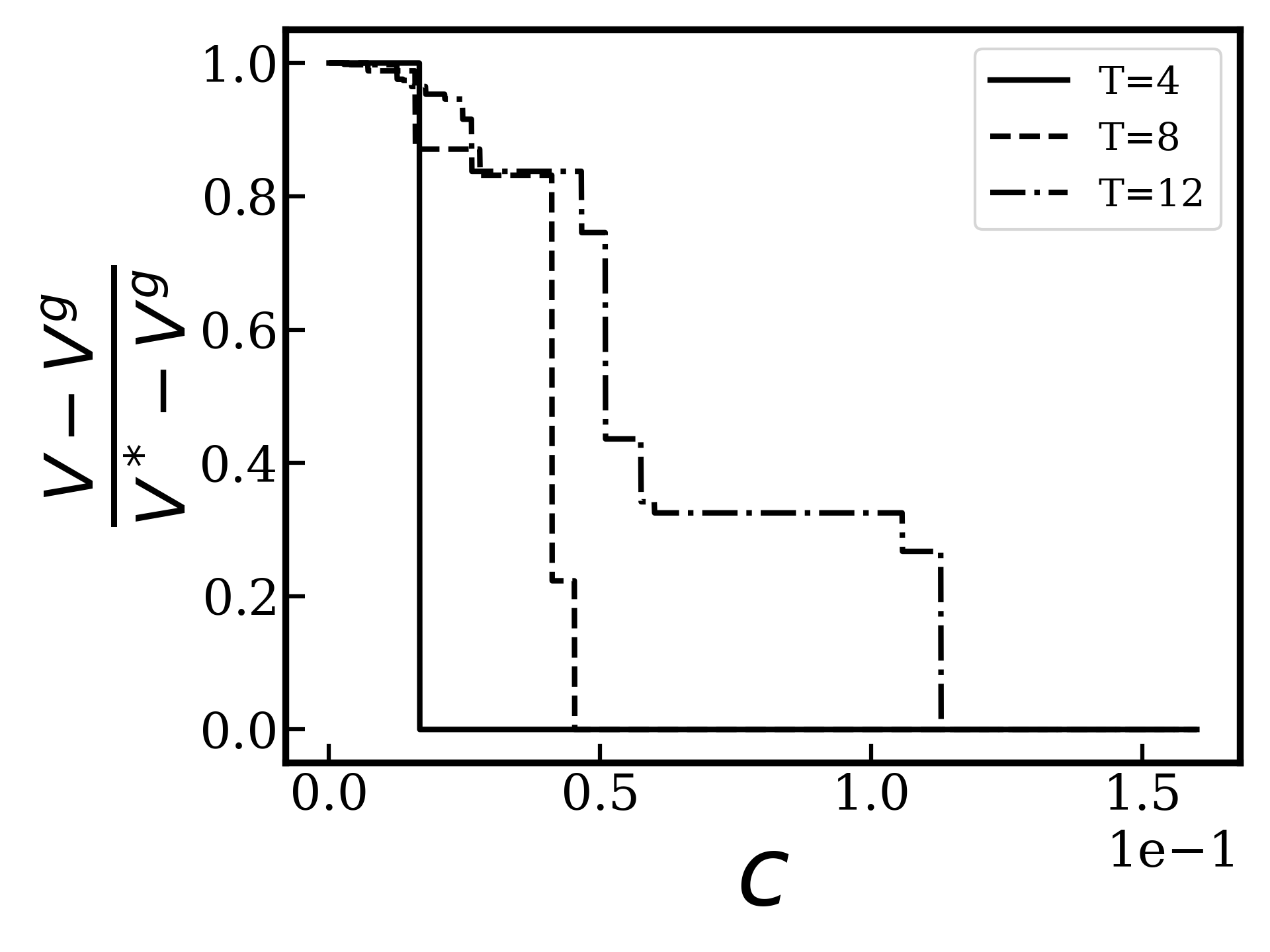
((a))

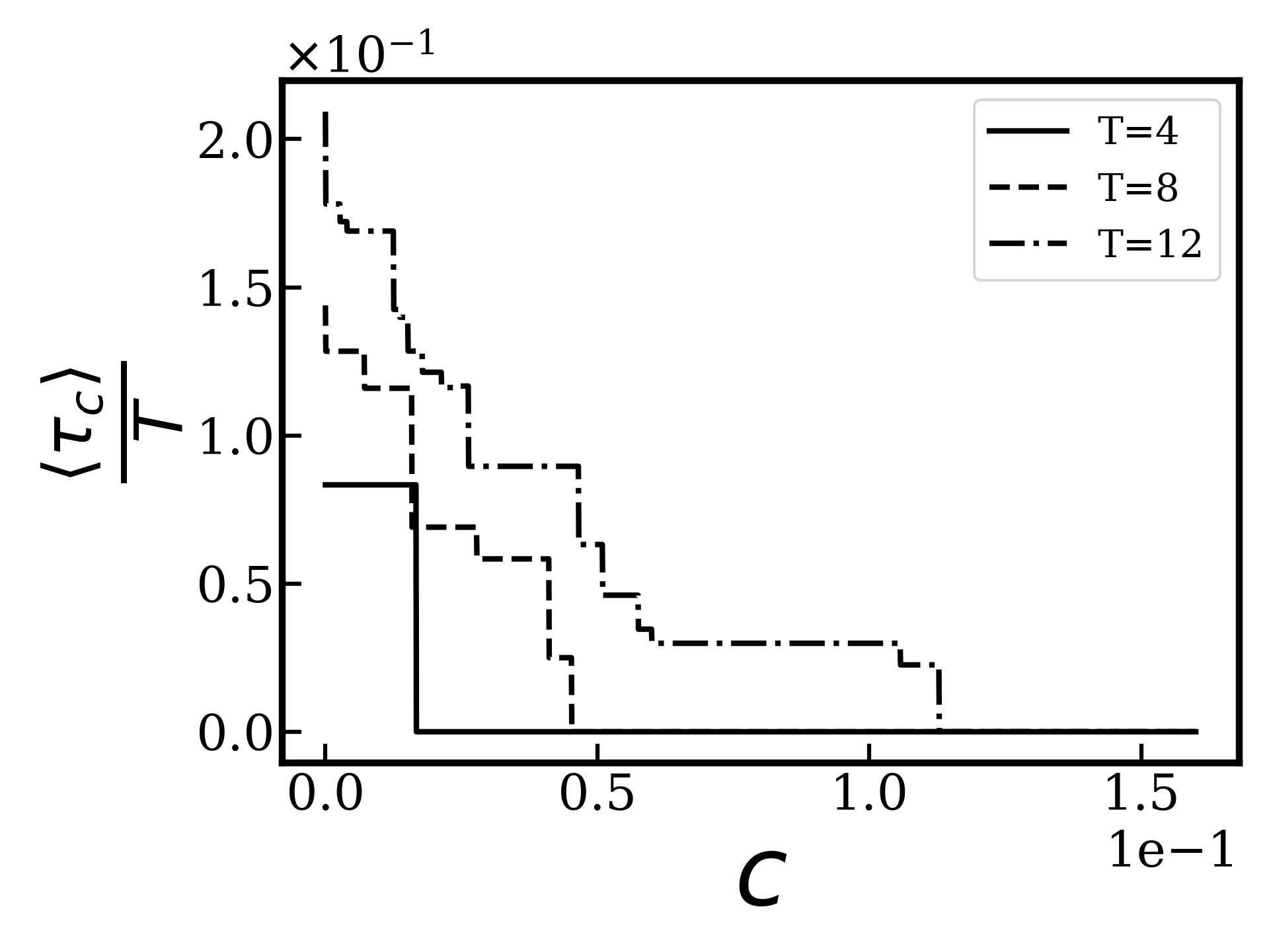
((b))

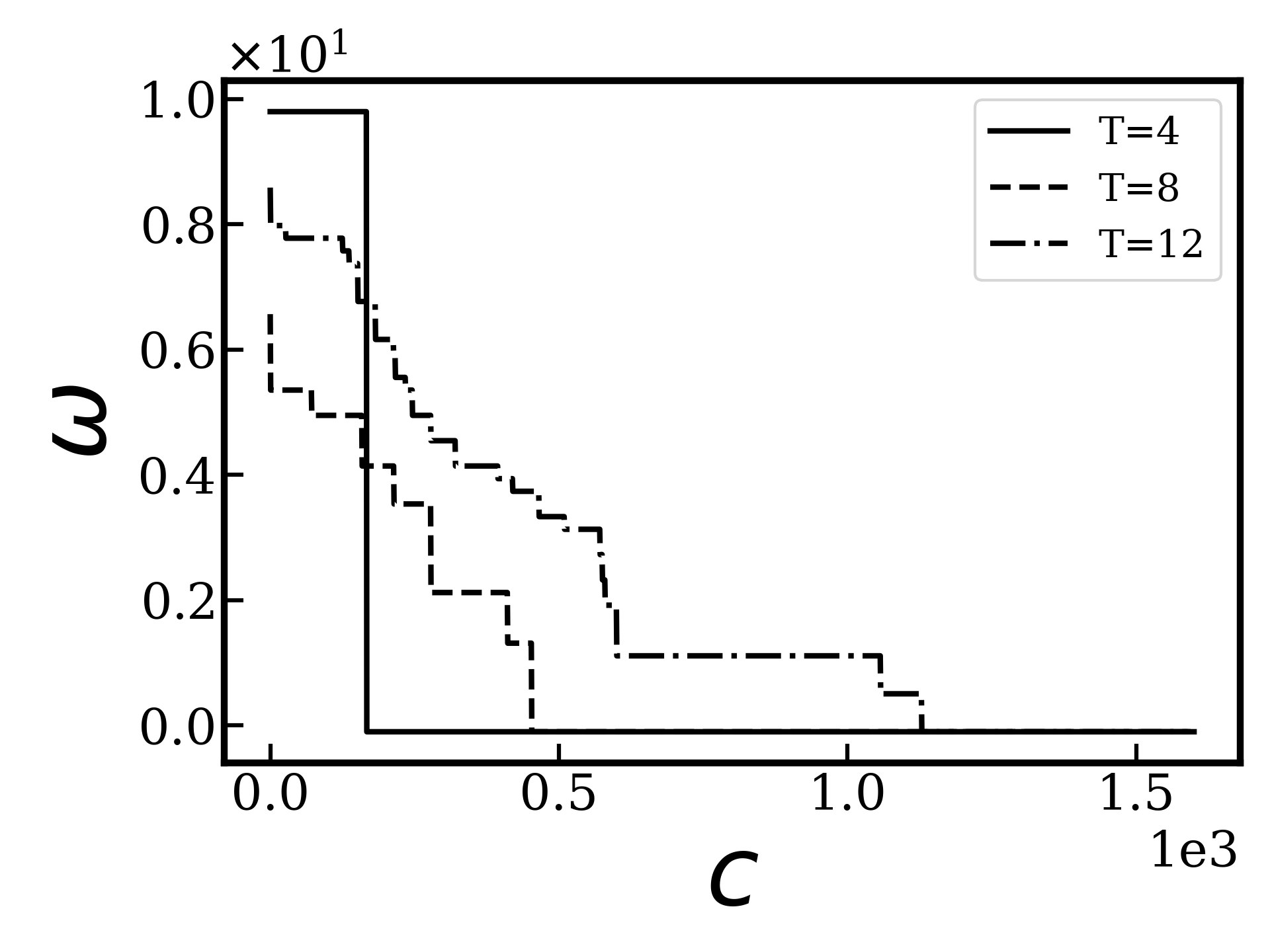
((c))

Figure 2: (a) Normalized, total expected reward accrued under the optimal meta-policy for a given computational cost and different task lengths. (b) Average time-step (in the TABB task) at which a node-expansion action is performed, as a function of the computational cost, for tasks of different lengths. (c) Coefficient for uncertainty based exploration (also called uncertainty bonus) for a given computational cost and different task lengths.

We discuss below the characteristic properties of the meta-BAMDP solutions for varying computational costs $c$, based on numerical solutions, for tasks of different lengths $T\leq 14$.

When comparing behavior in tasks of different lengths, we first consider the normalized expected reward (ignoring computational costs) under the optimal meta-policy as a function of computational cost (c.f. Fig. 2(a)). The presented values are averaged over a uniform distribution over all TABB environments. From Eq. 8 it is evident that the external rewards accrued by a meta-policy are lower bounded by the value of the greedy policy $V^{g}$ and upper bounded by the value of the optimal BAMDP policy, $V^{*}$. Therefore we define the normalized expected reward as $V^{N}=\frac{V-V^{g}}{V^{*}-V^{g}}$. We observe from Fig. 2(a) that $V^{N}$ monotonically decreases with $c$. This offers a novel computational explanation of the positive correlation observed between IQ and bandit task performance Steyvers et al. [2009], i.e individuals with higher working memory and attentional capacity have lower (opportunity-related) computational cost $c$ and therefore are able to plan further ahead and make better decisions. Additionally, we observe a characteristic dependence of behavior on the task horizon $T$. For shorter tasks, we find that the discrete jumps in the normalized value are higher. A systematic exploration of the dependence of human behavior on $T$ should be able to test such behavior.

To get more intuition about the behavior induced by the meta-policy, we consider $\langle\tau_{c}\rangle$, the average time step at which a computational action is performed. In Fig. 2(b) we see that as computational cost decreases, people explore until later in the task. Here we plot $\langle\tau_{c}\rangle$ normalized by the task horizon $T$. For high computational costs, agents perform only a few computations and they do so earlier on in the task. As inferring computational actions from experiments is non-trivial, we focus below on the behavioral consequence of being able to compute, i.e. exploratory actions.

We compare the qualitative features of the behavior induced by the solutions of the meta-BAMDP and human behavior in Bandit tasks. Specifically we consider the heuristic strategy from Brown et al. [2022], where an agent takes actions according to $\pi(a=i|\bm{b})\propto e^{-(\beta\hat{\mu}_{i}+\omega\hat{\sigma}_{i})}$, where $\hat{\mu}_{i},\hat{\sigma}_{i}$ are the estimated mean and variance of the belief distribution corresponding to state $\bm{b}$, i.e. a softmax policy based on a linear combination of expected reward and an “uncertainty bonus”. We fit this policy to the meta-policy obtained by solving the meta-BAMDP, and plot the corresponding value of $\omega$ (see Fig. 2(c)), the uncertainty bonus (for details see Sec. A.3). Qualitatively, we observe that, as computational costs increase, uncertainty driven exploration decreases, which is in line with experimental studies (Wu et al. [2022]). Additionally, we also find that generally, increasing $T$ also increases $\omega$ (for a fixed computational cost), which also matches well with the experimental observations (Wilson et al. [2014], Brown et al. [2022]). To our knowledge, ours is the first formal model that provides a normative explanation for the aforementioned set of empirical observations.

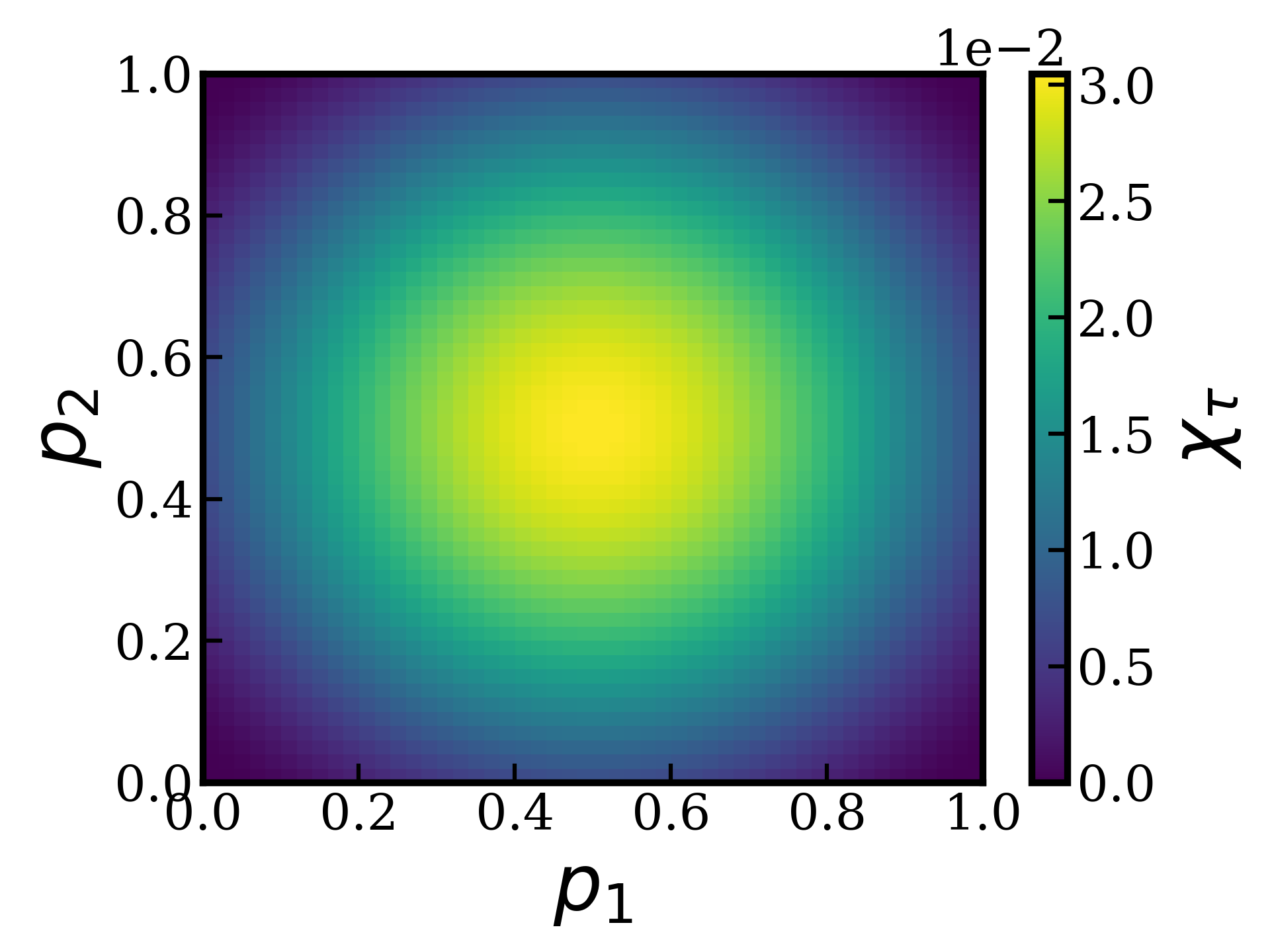
((a))

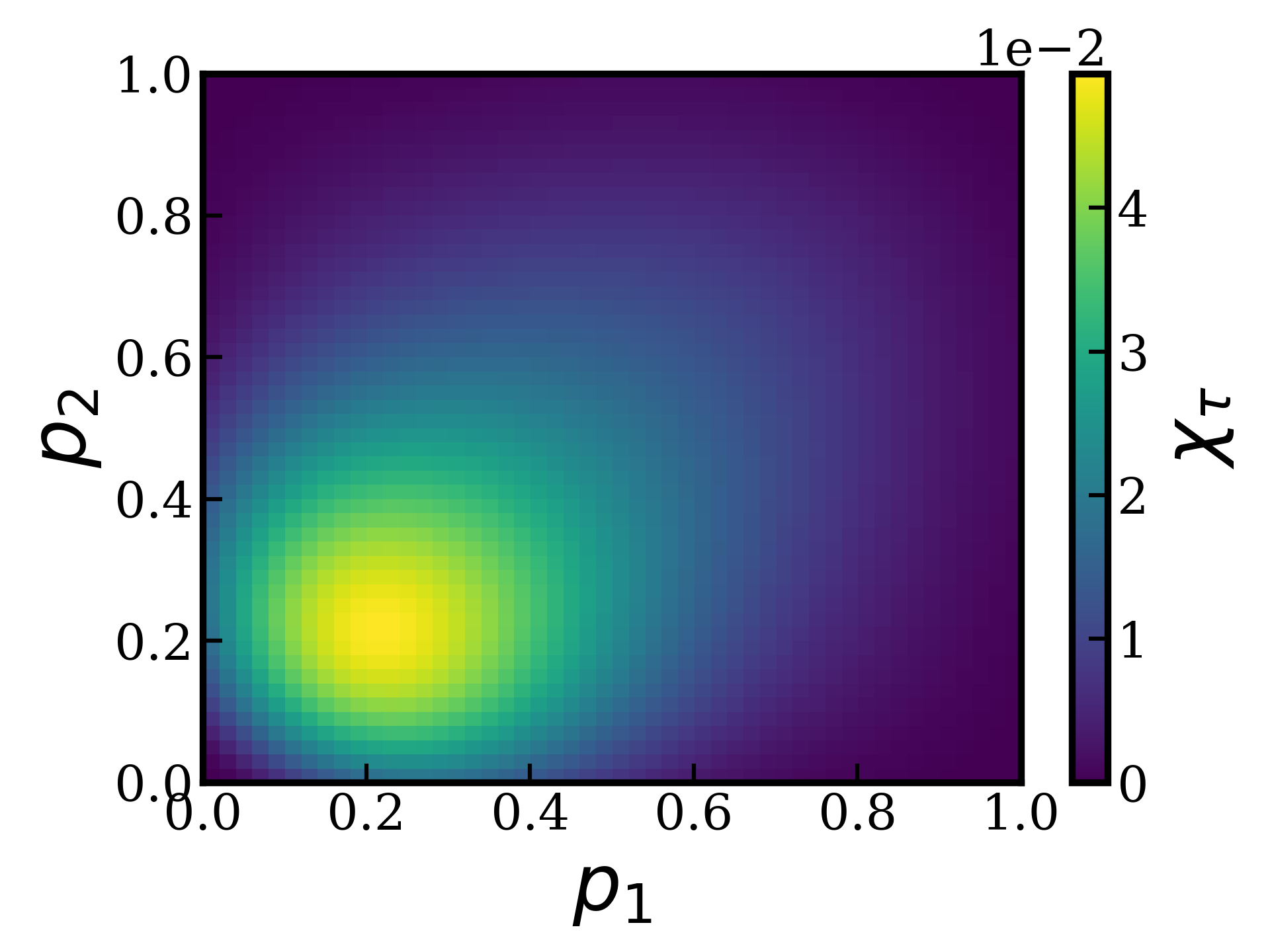
((b))

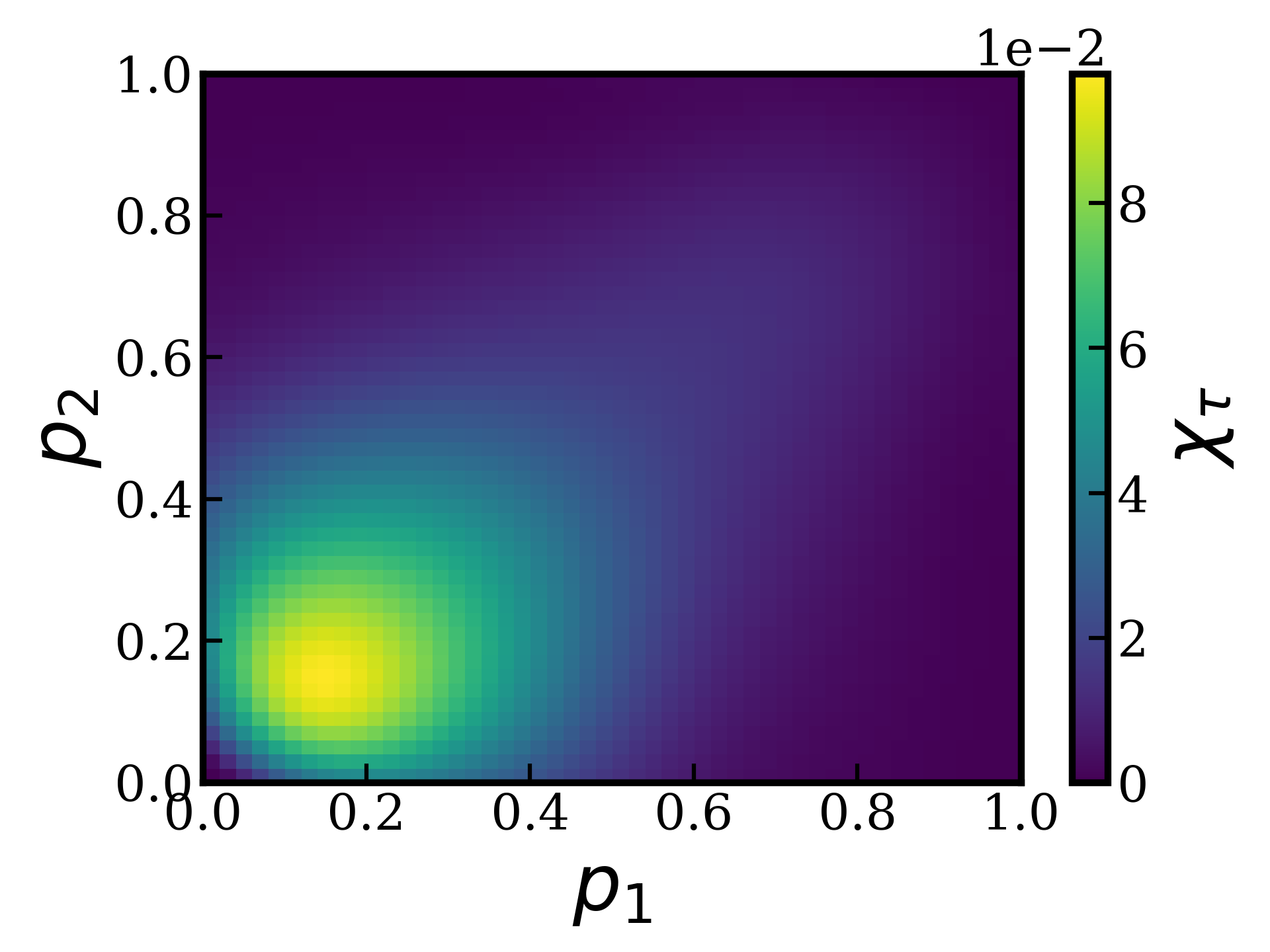
((c))

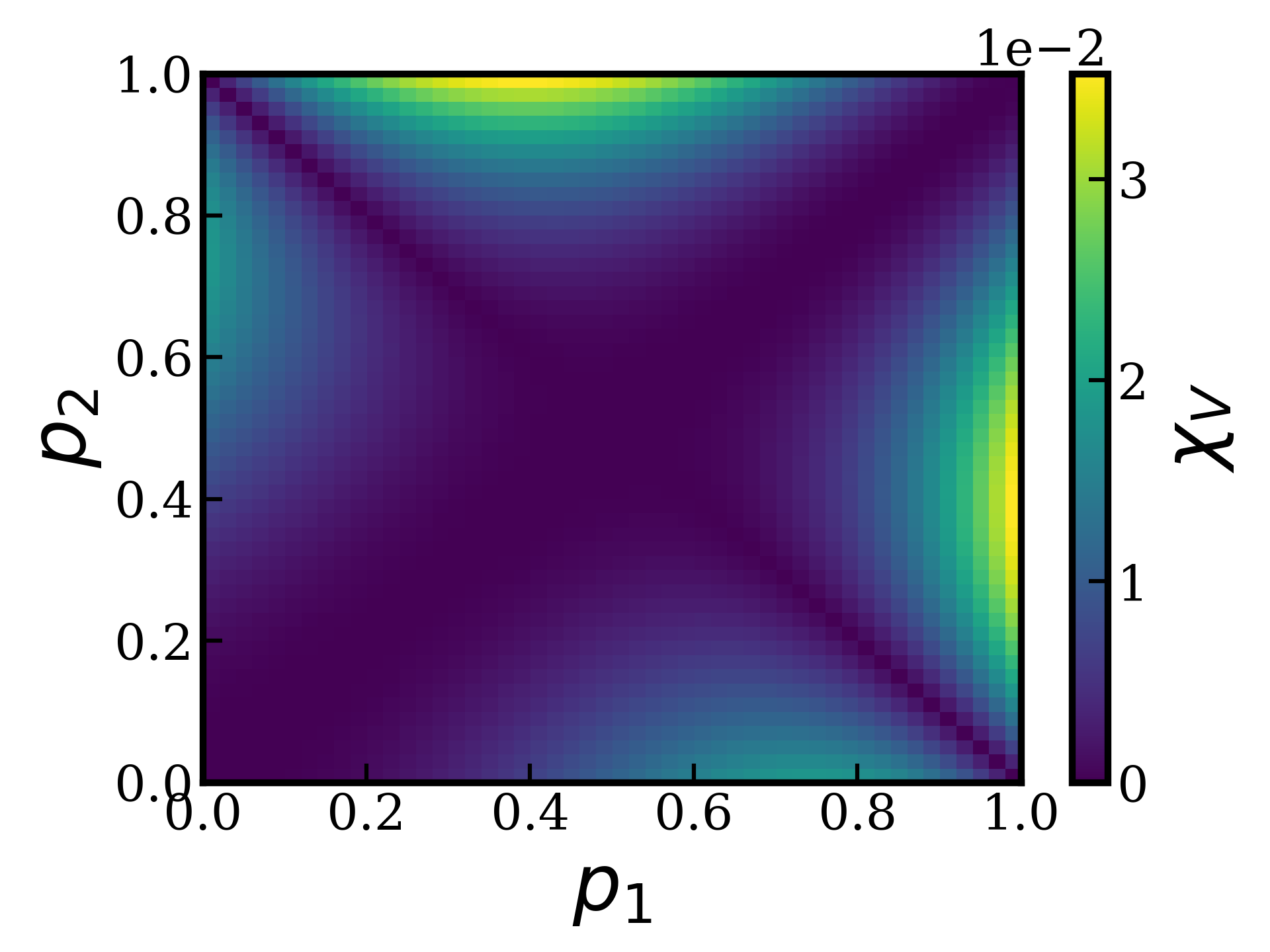
((d))

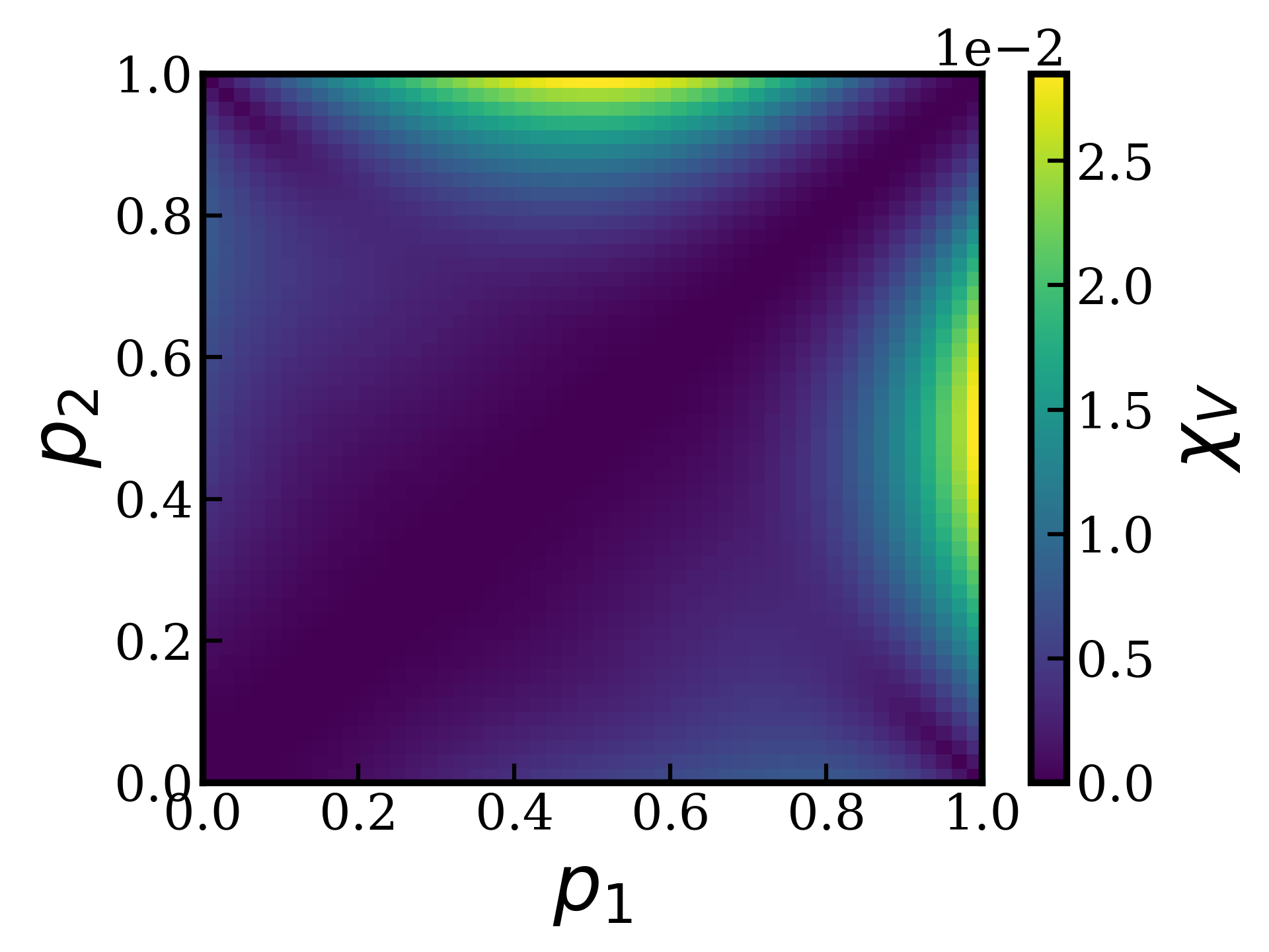
((e))

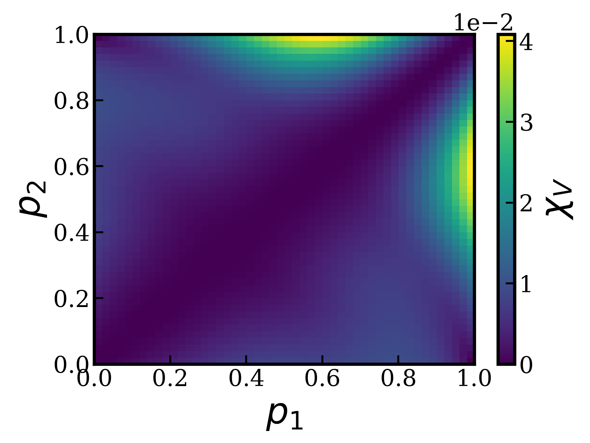
((f))

Figure 3: (a,b,c) Sensitivity of average time at which exploratory actions are taken, to changes in computational cost, for different task lengths. (d,e,f) Sensitivity of total expected reward to changes in computational cost, for different task lengths.

Finally, our model also provides testable predictions for resource bounded exploration in TABB tasks. For this we define two new quantities $\chi_{\tau},\chi_{V}$ which denote the sensitivity of $\tau,V$ respectively, to changes in computational costs. More precisely $\chi_{X}=\int dc(\frac{dX}{dc})^{2}$, for some observable $X$. Here, $\tau$ represents the average time step at which the agent performs an exploratory action, and $V$ is the total expected reward obtained by the agent (averaged over multiple runs for a given environment). In Fig. 3 we show $\chi_{\tau},\chi_{V}$ as a function of the environment $(p_{1},p_{2})$. We see that $\chi_{\tau}$ is maximized (yellow colored regions) for larger $T$ in increasingly reward-scarce environments (i.e. when $p_{1},p_{2}\leq 0.5$). On the other hand $\chi_{V}$ is maximized in reward-abundant environments (i.e. when $p_{1}+p_{2}\geq 1$), while the $p_{i}$ values are sufficiently distinct. For suitable assumptions about the distribution of $c$ in the test population, this might suggest observing a greater variance in $\chi_{\tau},\chi_{V}$ for environments chosen in the yellow regions, as compared to blue regions. Alternatively, these effects might be observable via an explicit control on $c$ through direct experimental manipulation, for instance, by imposing time constraints.

7 Conclusions

In this paper we developed a novel meta-BAMDP framework, which extends the scope of modeling metareasoning in humans to also include situations with unknown transition/reward dynamics. We present a theoretical instantiation of the framework in the TABB task, and provide an approach to make the problem computationally feasible. Moreover, we show that solutions from our model qualitatively explain recent experimental data on human exploration behavior in bandit tasks. Finally, our model also provides novel testable predictions for human behavior in bandit tasks. While additional work is needed to validate model predictions, as well as expanding theoretical understanding and practical implementation of a broader class of meta-BAMDP problems, this work nevertheless represents a novel theoretical and algorithmic advancement in reinforcement learning and human cognitive modeling.

Appendix A Supplementary material

The complete algorithm can be accessed via the url : https://github.com/Dies-Das/meta-BAMPD-data.

A.1 Pseudocode

The algorithm to find the solution to the meta-BAMDP involves two routines. First, to generate a pruned meta-graph and second to perform backward induction on this meta-graph, to find the optimal meta-policy. The latter is rather straight-forward, but the former is slightly complex to present and therefore for ease of understanding we provide a pseudocode below.

Input: maximum horizon $T$, initial beliefs $\bm{b}_{0}$, initial computational beliefs $\tilde{b}_{0}$, set $\mathcal{M}$

Output: pruned meta-graph $G$

1. Initialize the meta-graph $G$ with a root node containing $(\bm{b}_{0},\tilde{b}_{0})$.

2. Initialize a queue $Q$ and enqueue the root node.

3. While $Q$ is not empty:

   1. Dequeue a node $(\bm{b},\tilde{b})$ from $Q$.

   2. Determine the terminal action $a^{*}$ for $(\bm{b},\tilde{b})$ using Eq. 5.

   3. Calculate the subsequent belief states $\bm{b}^{\prime}$ for action $a^{*}$.

   4. Update $\tilde{b}^{\prime}$ to be the subgraph of $\tilde{b}$ starting from $\bm{b}^{\prime}$.

   5. Create new nodes $(\bm{b}^{\prime},\tilde{b}^{\prime})$ for the meta-graph $G$ if not already present.

   6. Add edges from $(\bm{b},\tilde{b})$ to $(\bm{b}^{\prime},\tilde{b}^{\prime})$.

   7. Enqueue new nodes $(\bm{b}^{\prime},\tilde{b}^{\prime})$ into $Q$.

   8. If $\bm{b}$ is not in $\mathcal{M}$:

      1. Start searching through all possible computational expansion trajectories from $(\bm{b},\tilde{b})$ to $(\bm{b},\tilde{b}^{\prime})$ that end with a terminal action. This is done by a depth-first search, while making use of the restrictions presented in Sec. 5.

      2. For each trajectory in the above set:

         1. Determine the terminal action $a^{**}$ and the subsequent belief states after executing $a^{**}$ in $(\bm{b},\tilde{b}^{\prime})$, i.e., $(\bm{b}^{\prime},\tilde{b}^{\prime\prime})$.

         2. If the $a^{**}$ differs from $a^{*}$, add the new nodes $(\bm{b}^{\prime},\tilde{b}^{\prime\prime})$ to $G$ and $Q$.

         3. Terminate the search along a trajectory if:

            • No further computations along this trajectory can change the physical action taken under that computational belief (Sec. 5).

            • Some other terminal condition X is met (see Sec. A.2).

4. Return the pruned meta-graph $G$.

There are two underdiscussed aspects of this pseudocode. First is that we only consider those computational action trajectories starting from $(\bm{b},\tilde{b})$ that can cause a change in the terminal action (as in 3.8.2.2. in the pseudocode above). There is no utility in performing computations if they cannot alter the terminal action, as any such computations could be done at a later state $\bm{b}^{\prime}$. Secondly, in the main manuscript, we assume that the terminal action leaves the $\tilde{b}$ unchanged. It should be easy to see that the only relevant part of $\tilde{b}$ in a state $(\bm{b},\tilde{b})$ is the reachable subgraph of $\bm{b}$, i.e. only computations about the reachable future are of relevance to the agent. Therefore, keeping the $\tilde{b}$ invariant to terminal actions or keeping only the relevant reachable subgraph are equivalent insofar as the solution to the meta-BAMDP is concerned.

A.2 Robustness of solution

In order to test the robustness of the approximate solution, we loosen the restriction of myopic approximation from Sec. 5, in two directions. These two directions, correspond to two distinct approximation schemes (or terminal conditions X above) that we tested. First as in the main text, we upper bound the maximum size $|\tilde{b}|$ of a computational belief $\tilde{b}$ that the agent can posses in any state by $k$. This may be viewed as bounding the working memory of an agent. Alternatively, we could also restrict the maximum number of computational actions $k_{c}$ that the agent is allowed to take between two consecutive terminal actions.

While staying within the bounds of the computational resources at our disposal, we find that the optimal solution remains invariant for $k_{c}\in\{1,2,3\}$ and for $2\leq k\leq 16$, as long as $T\leq 14$. For $T\geq 15$, $k=2$ or $k_{c}=1$ is no longer sufficient to obtain optimal behavior in the limit of $c\to 0$, thereby making the computation costly. We therefore leave computing the solution for larger $T$ for future work.

A.3 Comparing heuristics to meta-policies

For each computational cost $c$, we solve the meta-BAMDP problem and find the optimal meta-policy. Each meta policy implies a probability distribution over base policies. However, for the myopic assumption, each meta-policy has a unique corresponding base-policy, which we call $\pi^{\text{base}}(a|\bm{b})$. We define the squared distance between two base-policies $(\pi_{1},\pi_{2})$ to be $d^{2}(\pi_{1},\pi_{2})=\sum_{\bm{b}}\sum_{a}(\pi_{1}(a|\bm{b})-\pi_{2}(a|\bm{b}))^{2}$. In order to find the best fit $\omega$ (and simultaneously $\beta$), we minimize the squared distance $d^{2}(\pi_{1},\pi_{2})$ where $\pi_{1}\equiv\pi^{\text{base}}$ and $\pi_{2}\equiv\frac{1}{N}e^{-(\beta\hat{\mu}+\omega\hat{\sigma})}$, where $N$ is the normalization factor. As the optimal policies from the BAMDP are deterministic (except when ties are broken), the estimated value $\beta$ turns out to be suitably large ($\approx 100$ in our case). We consider the $\beta\times\omega$ space to be bounded by the square $(0,100)\times(-10,10)$, to remain broadly consistent with the work of Brown et al. [2022].

References

- Russell and Wefald [1991] Stuart Russell and Eric Wefald. Principles of metareasoning. Artificial Intelligence, 49(1):361–395, 1991. ISSN 0004-3702. doi: https://doi.org/10.1016/0004-3702(91)90015-C. URL https://www.sciencedirect.com/science/article/pii/000437029190015C.
- Hay et al. [2014] Nicholas Hay, Stuart Russell, David Tolpin, and Solomon Eyal Shimony. Selecting computations: Theory and applications. arXiv preprint arXiv:1408.2048, 2014.
- Mercer and Sampson [1978] Robert E Mercer and JR Sampson. Adaptive search using a reproductive meta-plan. Kybernetes, 7(3):215–228, 1978.
- Smit and Eiben [2009] S.K. Smit and A.E. Eiben. Comparing parameter tuning methods for evolutionary algorithms. In 2009 IEEE Congress on Evolutionary Computation, pages 399–406, 2009. doi: 10.1109/CEC.2009.4982974.
- Huang et al. [2019] Changwu Huang, Yuanxiang Li, and Xin Yao. A survey of automatic parameter tuning methods for metaheuristics. IEEE transactions on evolutionary computation, 24(2):201–216, 2019.
- Lieder et al. [2018] Falk Lieder, Amitai Shenhav, Sebastian Musslick, and Thomas L Griffiths. Rational metareasoning and the plasticity of cognitive control. PLoS computational biology, 14(4):e1006043, 2018.
- Callaway et al. [2022] Frederick Callaway, Bas van Opheusden, Sayan Gul, Priyam Das, Paul M Krueger, Thomas L Griffiths, and Falk Lieder. Rational use of cognitive resources in human planning. Nature Human Behaviour, 6(8):1112–1125, 2022.
- Lieder et al. [2014] Falk Lieder, Dillon Plunkett, Jessica B Hamrick, Stuart J Russell, Nicholas Hay, and Tom Griffiths. Algorithm selection by rational metareasoning as a model of human strategy selection. Advances in neural information processing systems, 27, 2014.
- D’Oro and Bacon [2021] Pierluca D’Oro and Pierre-Luc Bacon. Meta dynamic programming. In NeurIPS Workshop on Metacognition in the Age of AI: Challenges and Opportunities, 2021.
- Sutton [1991] Richard S Sutton. Dyna, an integrated architecture for learning, planning, and reacting. ACM Sigart Bulletin, 2(4):160–163, 1991.
- Lin et al. [2015] Christopher H Lin, Andrey Kolobov, Ece Kamar, and Eric Horvitz. Metareasoning for planning under uncertainty. arXiv preprint arXiv:1505.00399, 2015.
- Duff [2002] Michael O’Gordon Duff. Optimal Learning: Computational procedures for Bayes-adaptive Markov decision processes. University of Massachusetts Amherst, 2002.
- Zhang and Yu [2013] Shunan Zhang and Angela J Yu. Forgetful bayes and myopic planning: Human learning and decision-making in a bandit setting. Advances in neural information processing systems, 26, 2013.
- Steyvers et al. [2009] Mark Steyvers, Michael D. Lee, and Eric-Jan Wagenmakers. A bayesian analysis of human decision-making on bandit problems. Journal of Mathematical Psychology, 53(3):168–179, 2009. ISSN 0022-2496. doi: https://doi.org/10.1016/j.jmp.2008.11.002. URL https://www.sciencedirect.com/science/article/pii/S0022249608001090. Special Issue: Dynamic Decision Making.
- Brown et al. [2022] Vanessa M. Brown, Michael N. Hallquist, Michael J. Frank, and Alexandre Y. Dombrovski. Humans adaptively resolve the explore-exploit dilemma under cognitive constraints: Evidence from a multi-armed bandit task. Cognition, 229:105233, 2022. ISSN 0010-0277. doi: https://doi.org/10.1016/j.cognition.2022.105233. URL https://www.sciencedirect.com/science/article/pii/S0010027722002219.
- Wu et al. [2022] Charley M Wu, Eric Schulz, Timothy J Pleskac, and Maarten Speekenbrink. Time pressure changes how people explore and respond to uncertainty. Scientific reports, 12(1):4122, 2022.
- Wilson et al. [2014] Robert C Wilson, Andra Geana, John M White, Elliot A Ludvig, and Jonathan D Cohen. Humans use directed and random exploration to solve the explore–exploit dilemma. Journal of experimental psychology: General, 143(6):2074, 2014.
- Sutton and Barto [2018] Richard S Sutton and Andrew G Barto. Reinforcement learning: An introduction. MIT press, 2018.
- Huys et al. [2012] Quentin JM Huys, Neir Eshel, Elizabeth O’Nions, Luke Sheridan, Peter Dayan, and Jonathan P Roiser. Bonsai trees in your head: how the pavlovian system sculpts goal-directed choices by pruning decision trees. PLoS computational biology, 8(3):e1002410, 2012.
- Frazier et al. [2008] Peter I Frazier, Warren B Powell, and Savas Dayanik. A knowledge-gradient policy for sequential information collection. SIAM Journal on Control and Optimization, 47(5):2410–2439, 2008.