Strong Gravitational Lensing Effects and Observational Behaviors of the Rotating Short-Hairy Black Hole

Abstract

The successful capture of black hole(BH) images by the Event Horizon Telescope(EHT) has sparked a surge in research on strong gravitational lensing, providing new methods for studying behavior near the event horizon of BHs. For the short-hair that has significant effects only near the BH event horizon, studying its strong gravitational lensing effects helps to understand the nature of this hair. This paper explores the behaviors of the rotating short-hairy BH in strong gravitational lensing. Simulations show that the short-hair parameter results in a smaller event horizon radius, photon sphere, and impact parameter compared to the Kerr BH. Moreover, the lensing coefficients $\bar{a}$ and $\bar{b}$ show opposite trends due to the short-hair parameter $Q_{m}$, with the former increasing and the latter decreasing. It is worth mentioning that in certain cases, the short-hair parameter can make $\bar{b}$ slightly higher than that of the Kerr BH. The deflection angle $\alpha_{D}$ decreases with an increasing impact parameter and diverges at $u_{m}$, with the divergent impact parameter of rotating short-hairy BH being smaller than that of the Kerr BH. In the context of $M87^{*}$ and $SgrA^{*}$ BHs, their Einstein rings, relativistic images, and time delays differ significantly from those of the Kerr BH. Although current equipment cannot yet distinguish these differences, future high-precision instruments are expected to achieve this goal, thereby differentiating rotating short-hairy BH from the Kerr BH, exploring the nature of the short-hair, and testing the no-hair theorem of BH. This provides a new perspective for understanding the extreme physical environments of BHs and offers necessary references for future observational and theoretical research.

Keywords

Strong Gravitational Lensing; Rotating Short-Hairy Black Hole; No-Hair Theorem

I Introduction

The general theory of relativity predicts the existence of black holes, but finding evidence of BH in the real universe is crucial for validating this theory. This has greatly stimulated the interest of physicists. In September 2015, the LIGO detector first captured gravitational wave signals produced by the merger of two BHs, providing strong evidence for the success of general relativity LIGOScientific:2016emj . In the real universe, most of the observed astrophysical BHs are rotating and fit well with the Kerr metric Teukolsky:2014vca ; Tao:2023hou . However, this does not rule out the possibility of a range of Kerr-like BHs Azreg-Ainou:2014pra ; Ghosh:2014pba . In fact, as Xu and Tang stated in the literature Xu:2021dkv , Kerr BH serving as astrophysical BH in the real universe is not entirely applicable. This is because BH in the real universe do not exist in isolation but are coupled with dark matter or other forms of fields, making the real universe more complex. Therefore, accurately describing astrophysical BH using standard Kerr black holes may present certain challenges.

If a type of Kerr-like BH solution that considers coupling with anisotropic matter could be found to describe astrophysical BH, it might be more meaningful. The short-hairy BH solution provided in the literature Brown:1997jv better fits the real universe environment because their short-hairy BH solution considers BH solutions coupled with anisotropic matter. Their static spherically symmetric BH solution violates the no-hair theorem. The no-hair theorem states Hawking:1971vc ; Israel:1967wq that within the framework of general relativity, the properties of a BH can be completely described by three parameters: mass $M$, charge $Q$, and angular momentum $J$. However, once Einstein’s gravity is coupled with other matter, BH solutions that violate the no-hair theorem may appear Lee:2018zym ; Greene:1992fw ; Bizon:1990sr ; Ovalle:2020kpd . Therefore, studying the properties of short-hairy BH solutions Brown:1997jv would be very interesting. However, the BH solution they provided is static and spherically symmetric. It would be more valuable to extend this solution to the rotating and axisymmetric case. This is because, on the one hand, most astrophysical BHs are rotating, so a rotating solution can better match astrophysical BHs. On the other hand, jet phenomena are common around rotating BHs, and observing these jets helps us study and understand the physical behavior near the event horizon, especially for this type of short hair that has a significant impact near the event horizon. Based on this objective, Tang and Xu in 2022 used the Newman-Janis (NJ) algorithm to extend the short-hairy BH to the case of rotating short-hairy BH, and they also studied the impact of short-hair parameter on the BH shadow Tang:2022uwi . Studying other properties of the rotating short-hairy BH is also very meaningful. For example, exploring their physical behavior under strong gravitational lensing can help us further understand the characteristics of rotating short-hairy BH and provide a window to test the no-hair theorem.

Gravitational lensing is an important tool for studying BHs (or other massive objects) and their surrounding environments. It has been widely applied in understanding the structure of spacetime Liebes:1964zz ; Mellier:1998pk ; Guzik:2009cm ; Schmidt:2008hc , has played a significant role in the search for dark matter Massey:2010hh ; Vegetti:2023mgp ; DiazRivero:2019hxf ; Sengul:2022edu ; Fairbairn:2022xln , and is also an effective means of testing gravitational theories Zhao:2024elr ; Bekenstein:1993fs ; Islam:2020xmy ; Kumar:2020sag ; Chen:2009eu . In strong gravitational fields, such as near a BH, when light approaches the BH (especially near the photon sphere), the light can be strongly bent and may even orbit the black hole one or more times, with the deflection angle exceeding $2\pi$. In such cases, shadows, photon rings, and relativistic images can appear Gralla:2019xty ; Bozza:2010xqn ; Bozza:2001xd ; Bozza:2002af . Regarding strong gravitational lensing, Virbhadra and Ellis analyzed the strong gravitational effects caused by a Schwarzschild BH through numerical simulations Virbhadra:1999nm . Subsequently, Bozza Bozza:2001xd ; Bozza:2002zj ; Bozza:2010xqn and Tsukamoto Tsukamoto:2016jzh extended this to general static spherically symmetric spacetimes. Naturally, other static spherically symmetric BHs have also been studied accordingly Man:2012ivp ; Wei:2014dka ; Eiroa:2013nra ; Eiroa:2012fb ; Eiroa:2005ag ; Eiroa:2004gh ; Zhao:2017cwk ; Zhao:2024elr . Additionally, rotating axisymmetric BHs have also received extensive attention Bozza:2008mi ; Bozza:2010xqn ; Bozza:2002af ; Wei:2011nj ; Islam:2021dyk ; Islam:2021ful ; Hsiao:2019ohy .

In fact, in 2019, the EHT successfully captured images of the supermassive BH $M87^{*}$ EventHorizonTelescope:2019dse , and in 2022, it captured images of the BH at the center of the Milky Way, $SgrA^{*}$ EventHorizonTelescope:2022wkp . These groundbreaking observations have sparked a surge of interest in studying strong gravitational lensing. The EHT’s observations provide a new laboratory for studying the properties of black holes, such as the black hole’s shadow, the jet phenomenon of the accretion disk, the event horizon, and other properties that previously could only be theoretically calculated but can now be verified through observation. Naturally, studying the strong gravitational lensing effects around BH is also of great significance, as it can magnify and distort the images of background celestial bodies, providing a unique method to detect BHs and their surrounding material distribution. Therefore, studying strong gravitational lensing in BHs that are more akin to those in the real universe holds greater physical value. The environment considered for the rotating short-hairy BH Tang:2022uwi is more similar to the real universe (anisotropic matter). Studying strong gravitational lensing in such BH can help us test the no-hair theorem, distinguish Kerr BH, and further understand the properties of short-hair near the event horizon. For this kind of hair, which has significant effects near the event horizon but is difficult to observe for distant observers, observing the behavior of light reaching near the event horizon will help us better understand the properties of this short-hair.

The organization of this paper is as follows: In Section II, we briefly introduce the short-hairy black hole and its event horizon information. In Section III, we calculate the lensing coefficients for $k=1,1.5,2$ and explore the impact of the short-hair parameter $Q_{m}$ on the lensing. In Section IV, we discuss the lensing observational effects of the rotating short-hairy black hole, considering it as a candidate for the supermassive BHs $M87^{*}$ and $SgrA^{*}$. We study Einstein rings, relativistic images, and time delays on the same side. The final section presents the results. Throughout the article, we use natural units where $c=G=\hbar=1$.

II Quantum-corrected black hole

In the framework of classical general relativity, the no-hair theorem states that the properties of a BH can be fully described by just three parameters: mass $M$, charge $Q$, and angular momentum $J$ Hawking:1971vc ; Israel:1967wq . However, just as many researchers test the cosmic censorship conjecture in different settings Frassino:2024fin ; Zhao:2023vxq ; Meng:2023vkg ; Zhao:2024lts ; Jiang:2023xca ; Meng:2024els ; Zhao:2024qzg ; Cao:2024kht , many scholars are also keen to find examples that violate the no-hair theorem. In the 1990s, Piotr Bizon obtained a ”hairy” BH solution through numerical analysis, marking the first discovered violation of the no-hair theorem Bizon:1990sr . This discovery motivated further searches for more counterexamples to this theorem. For instance, Ovalle et al. obtained a spherically symmetric spacetime solution with hair using the gravitational decoupling method Ovalle:2020kpd , and subsequently, Contreras et al. extended this to the rotating case Contreras:2021yxe . Other BH solutions with scalar hair are described in the literature Carames:2023pde ; Bakopoulos:2023hkh ; Zhang:2022csi ; Brihaye:2015qtu , and additional BH solutions obtained through the gravitational decoupling method can be found in Ovalle:2020kpd ; Ovalle:2018umz ; Avalos:2023ywb ; Ovalle:2023ref . In the literature Brown:1997jv , the authors obtained short-hairy BH solutions by coupling Einstein’s gravity with anisotropic matter. These solutions can present de Sitter and Reissner-Nordström BHs in some cases, and in others, they yield short-hairy BH solution Brown:1997jv . The corresponding metric is given by

$$f(r)=1-\frac{2M}{r}+\frac{Q_{m}^{2k}}{r^{2k}},$$ (1)

where $Q_{m}$ represents the strength parameter of the hair, i.e., the short-hair parameter, which has a significant impact near the event horizon.

This short-hairy BH is extremely special because the spacetime environment considered by these authors is neither vacuum nor isotropic but anisotropic. Physically, this is closer to the real universe. In other words, in our real universe, the conditions of vacuum or isolated systems do not exist. This also indicates that such BHs are more likely to occur in our real universe, making the discussion of the properties of this short-hairy BH more valuable.

Due to the fact that BHs or compact objects in the real universe are rotating, it would be more meaningful to extend this short-hairy BH to the rotating case. Therefore, in 2022, Tang and Xu used the Newman-Janis (NJ) algorithm to extend the metric of the static spherically symmetric short-hairy BH to the rotating case. They obtained the solution for a rotating short-hairy BH and studied the effect of the short-hair parameter on the BH shadow Tang:2022uwi . For this rotating short-hairy BH, studying other physical properties is also very valuable because the spacetime background considered for the rotating short-hair BH is closer to the real universe (the spacetime is non-vacuum, and the surrounding matter is anisotropic). The metric for the rotating short-hairy BH is as follows Tang:2022uwi

$$ds^{2} =-\left(1-\frac{2Mr-\frac{Q_{m}^{2k}}{r^{2k-2}}}{\rho^{2}}\right)dt^{2}+\frac{\rho^{2}}{\Delta}dr^{2}$$

$$-\frac{2a\sin^{2}\theta\left(2Mr-\frac{Q_{m}^{2k}}{r^{2k-2}}\right)}{\rho^{2}}dtd\phi+\rho^{2}d\theta^{2}$$

$$+\frac{\Sigma\sin^{2}\theta}{\rho^{2}}d\phi^{2},$$ (2)

where

$$\rho^{2}=r^{2}+a^{2}\cos^{2}\theta,$$ (3)

$$\Sigma=(r^{2}+a^{2})^{2}-a^{2}\Delta,$$ (4)

$$\Delta=r^{2}-2Mr+\frac{Q_{m}^{2k}}{r^{2k-2}}+a^{2}.$$ (5)

Here, $a$ represents the spin parameter of the BH, and $Q_{m}$ also represents the strength parameter of the hair, i.e., the short-hair parameter. As stated in the original paper Brown:1997jv , the short-hairy BH satisfies the weak energy condition (WEC), so the parameter $k$ must satisfy $2k-1\geq 0$, i.e., $k$ must be $\geq 1/2$. We note that when $k=1$, the metric (2) becomes the Kerr-Newman BH, which degenerates to the Reissner-Nordström BH in the static spherically symmetric case. When $k>1$, it represents a short-hairy BH. Specifically, when $k=1.5$, this metric represents a rotating BH with ”short hair.” When $k=2$, we note that the metric (2) degenerates to the static spherically symmetric short-hairy black hole (when $a=0$), and this metric is the same as the quantum-corrected BH metric recently proposed by Lewandowski et al. within the framework of quantum gravity Lewandowski:2022zce . Their spherically symmetric BH spacetime metric is $f(r)=1-\frac{2M}{r}+\frac{\alpha M^{2}}{r^{4}}$. The quantum-corrected BH solution proposed by Lewandowski et al. is a type of BH solution that avoids spacetime singularities Lewandowski:2022zce , and such solutions are very valuable. Therefore, obtaining the rotating version of this BH solution would be even more meaningful. We note that the metric of the rotating short-hairy BH can degenerate into their static spherically symmetric BH solution in specific cases, implying that the special case of the rotating short-hairy BH solution might be their metric extended to the rotating BH case, indirectly indicating the uniqueness of such short-hairy BH solutions. Therefore, in this paper, we will focus on discussing the cases of short-hairy BHs with parameters $k=1,3/2,2$.

To facilitate the following analysis, we dimensionless all physical parameters in metric (2) by using $2M$ as the unit (e.g., $r\to 2Mx$, etc.). When setting $M=1/2$, the corresponding metric becomes

$$ds^{2} =-\left(1-\frac{x-\frac{Q_{m}^{2k}}{x^{2k-2}}}{\rho^{2}}\right)dt^{2}+\frac{\rho^{2}}{\Delta}dx^{2}$$

$$-\frac{2a\sin^{2}\theta\left(2Mx-\frac{Q_{m}^{2k}}{x^{2k-2}}\right)}{\rho^{2}}dtd\phi+\rho^{2}d\theta^{2}$$

$$+\frac{\Sigma\sin^{2}\theta}{\rho^{2}}d\phi^{2},$$ (6)

where

$$\rho^{2}=x^{2}+a^{2}\cos^{2}\theta,$$ (7)

$$\Sigma=(x^{2}+a^{2})^{2}-a^{2}\Delta,$$ (8)

$$\Delta=x^{2}-x+\frac{Q_{m}^{2k}}{x^{2k-2}}+a^{2}.$$ (9)

For the parameter model we are discussing, the event horizon of a rotating short-hairy BH can be given by $g^{rr}=0$, that is, $\Delta=0$. Numerical simulations of equation (9) can yield the existence of the event horizon, as shown in Figure 1, depicting the event horizon of the rotating short-hairy BH under different conditions. In the figure, the black lines represent the event horizon in the absence of the short-hair parameter (Kerr BH). Clearly, even for different parameters $k$, the presence of the short-hair parameter$Q_{m}$ results in an event horizon smaller than that of the BH without hair.

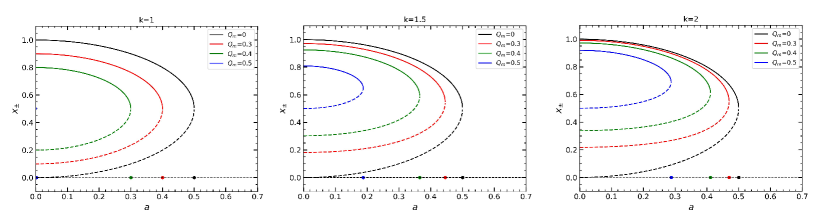
Figure 1: The event horizon and Cauchy horizon for different parameters, with solid lines representing the event horizon $r_{+}$ and dashed lines representing the Cauchy horizon $r_{-}$.

III Strong gravitational lensing under rotating short-hairy black hole

For the metric of a rotating BH, to facilitate the calculations, we confine the light rays to the equatorial plane, i.e., $\theta=\pi/2$. The spacetime line element can be written as

$$ds^{2}=-A(x)dt^{2}+B(x)dx^{2}+C(x)d\phi^{2}-D(x)dtd\phi.$$ (10)

By comparing the metric of a rotating short-hair black hole given in equations (6) and (10), we obtain

$$A(x) =\left(1-\frac{x-\frac{Q_{m}^{2k}}{x^{2k-2}}}{x^{2}}\right),$$ (11)

$$B(x) =\frac{x^{2}}{\Delta},$$ (12)

$$C(x) =\frac{\Sigma}{x^{2}},$$ (13)

$$D(x) =\frac{2a\left(x-\frac{Q_{m}^{2k}}{x^{2k-2}}\right)}{x^{2}}.$$ (14)

For the light rays confined to the equatorial plane, the corresponding Lagrangian is

$$L=\frac{1}{2}g_{\mu\nu}\frac{dx^{\mu}}{d\lambda}\frac{dx^{\nu}}{d\lambda},$$ (15)

where $\lambda$ is the affine parameter. Due to the axisymmetry of the rotating short-hairy BH, there are two conserved quantities: energy and angular momentum, given by

$$E=\frac{\partial L}{\partial\dot{t}}=-g_{tt}\dot{t}-g_{t\phi}\dot{\phi},$$ (16)

$$L=-\frac{\partial L}{\partial\dot{\phi}}=g_{t\phi}\dot{t}+g_{\phi\phi}\dot{\phi},$$ (17)

where the overdot represents differentiation with respect to the affine parameter, i.e., $d/d\lambda$. When choosing an appropriate affine parameter such that $E=1$, the equations of motion for light can be written as

$$\dot{t}=\frac{4C-2DL}{4AC+D^{2}},$$ (18)

$$\dot{\phi}=\frac{2D+4AL}{4AC+D^{2}},$$ (19)

$$\dot{x}=\pm 2\sqrt{\frac{C-DL-AL^{2}}{B(AC+D^{2})}}.$$ (20)

The effective potential can be defined through equation (20) as

$$V_{\text{eff}}(x)=-\dot{x}^{2}=-4\frac{C-DL-AL^{2}}{B(AC+D^{2})}.$$ (21)

By using the impact parameter $u=L/E=L$ to replace the angular momentum $L$, equation (21) can be written as

$$V_{\text{eff}}(x)=-4\frac{C-Du-Au^{2}}{B(AC+D^{2})}.$$ (22)

In the above expressions, $A$, $B$, $C$, and $D$ are all functions of $x$.

Clearly, according to the effective potential, when light from infinity reaches the vicinity of a rotating short-hairy BH, it cannot directly enter the BH due to the presence of the effective potential. Instead, when it reaches a specific radius $x_{0}$, the light will be deflected and eventually escape to infinity to be observed by distant observers. We note that when light reaches the vicinity of certain orbits around the BH, these orbits are extremely unstable. Small perturbations will cause the light to either fall into the BH or escape to infinity. These specific orbits are known as photon sphere orbits. For an unstable photon sphere, when light reaches its vicinity, the light will diverge to infinity. This unstable behavior leads to lensing effects and the BH shadow, with the lensing effect being the focus of this paper.

The condition for an unstable photon sphere is given by Harko:2009xf

$$\left.\frac{dV_{\text{eff}}(x)}{dx}\right|_{x_{m}}=0,\;\left.\frac{d^{2}V_{\text{eff}}(x)}{dx^{2}}\right|_{x_{m}}<0\;(\text{unstable photon sphere}).$$ (23)

Combining equations (22) and (23), the orbit equation for the unstable photon sphere can be derived as

$$A(x)C^{\prime}(x)-A^{\prime}(x)C(x)+u\left(A^{\prime}(x)D(x)-A(x)D^{\prime}(x)\right)=0.$$ (24)

Solving this equation yields the largest root $x_{m}$, which is the orbit radius of the unstable photon sphere. This can be easily obtained from the plot of the effective potential. As shown in Figure 2, when the impact parameter takes the critical value (indicated by the green dashed line), it corresponds to the radius of the unstable photon sphere in that situation ($\dot{x}=0$). In the following discussion, we take the radius of the unstable photon sphere as $x=x_{m}$. For the radius of the unstable photon sphere, it is evident that the presence of hair makes its radius significantly different. As shown in Figure 3, with the continuous increase of the spin parameter, the radius $x_{m}$ of the unstable photon sphere under different models gradually decreases (this radius is the radius of the unstable photon sphere). Additionally, due to the presence of the hair parameter $Q_{m}$, the $x_{m}$ of the rotating short-hairy BH is smaller than that of the Kerr BH (corresponding to $Q_{m}=0$). In the figure, the black dashed line represents the Kerr BH.

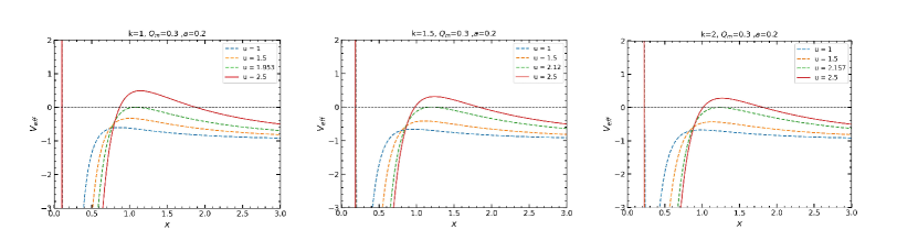
Figure 2: The effective potential functions for specific values under three models and the positions of the unstable photon rings are shown. The intersection points of the green dashed lines and the black dashed lines represent the positions of the unstable photon spheres. Here, $Q_{m}=0.3$ and $a=0.2$. From left to right, the BH models correspond to $k=1$, $k=1.5$, and $k=2$. We plot the effective potential under different short-hair parameter.

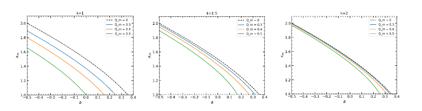
Figure 3: The variations of the radius of the unstable photon sphere with respect to the spin parameter $a$ and the short-hair parameter $Q_{m}$ for three models. From left to right, the BH models correspond to $k=1$, $k=1.5$, and $k=2$.

When light from infinity with a certain impact parameter $u$ approaches the black hole, it reaches the nearest point to the BH at a distance $x_{0}$. At this distance, the radial velocity of the light becomes zero while the angular velocity is non-zero. The light is symmetrically deflected to infinity at this point. Since the radial velocity of the photon is zero at this closest distance, the corresponding effective potential is zero, i.e., $V_{\text{eff}}(x)=0$ (as shown in Figure 2). The relationship between the impact parameter and the minimum distance $x_{0}$ can be derived from equation (22) as follows:

$$L =u(x_{0})=\frac{-D(x_{0})+\sqrt{4A(x_{0})C(x_{0})+D(x_{0})^{2}}}{2A(x_{0})}$$

$$=\frac{aQ_{m}^{2k}x^{2-2k}-ax+x^{2}\sqrt{a^{2}+Q_{m}^{2k}x^{2-2k}+x^{2}-x}}{Q_{m}^{2k}x^{2-2k}+x^{2}-x}.$$ (25)

In the above equation, $x_{0}$ represents the shortest distance. Since we are primarily interested in the behavior of light near the unstable photon sphere, $x_{0}\approx x_{m}$. Therefore, the impact parameter corresponding to the unstable photon sphere can be expressed as $u(x_{m})$. The relationship between $u(x_{m})$, the spin parameter $a$, and the short-hair parameter $Q_{m}$ can be obtained from Figure 4. It is evident that as the spin parameter $a$ or the short-hair parameter $Q_{m}$ increases, the corresponding impact parameter decreases continuously. Their variation trends are similar to those of the photon sphere orbit radius. Here, we define the direction of photon orbiting around the BH as counterclockwise. For the case where the spin parameter $a>0$ (the BH rotates counterclockwise), the direction of light orbiting is the same as the spin direction of the BH, which we call prograde orbit. Conversely, when the spin parameter $a<0$, the spin direction is opposite to the orbiting direction, which we call retrograde orbit. This also explains why the prograde orbit radius of the photon sphere is often smaller than the retrograde orbit radius (see Figure 3, for the prograde orbit radius, the dragging effect due to spin helps the photon to remain on an orbit closer to the BH, and vice versa).

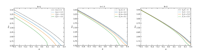
Figure 4: The variations of the impact parameter with respect to the spin parameter $a$ and the short-hair parameter $Q_{m}$ for three models. From left to right, the black hole models correspond to $k=1$, $k=1.5$, and $k=2$.

In the strong field limit, the deflection angle $\alpha_{D}$ can be given by Bozza:2002zj ; Bozza:2002af

$$\alpha_{D}(x_{0})=I(x_{0})-\pi,$$ (26)

where

$$I(x_{0}) =2\int_{x_{0}}^{\infty}\frac{d\phi}{dx}dx$$

$$=2\int_{x_{0}}^{\infty}\frac{\sqrt{A_{0}B}(2Au+D)}{\sqrt{4AC+D^{2}}\sqrt{A_{0}C-AC_{0}+u(AD_{0}-A_{0}D)}}dx.$$ (27)

Here, to facilitate the notation, all capital letters in this paper represent functions of $x$, and all letters with the subscript ”0” correspond to functions evaluated at $x=x_{0}$.

Analyzing the integral in equation (27), it becomes apparent that for certain values, the integral is divergent. To address this issue, we adopt a straightforward and effective method, namely, expanding the deflection angle near the unstable photon sphere Bozza:2002zj ; Tsukamoto:2016jzh . Naoki Tsukamoto’s redefined intermediate variable for the strong field limit is used to resolve the divergence problem, which can be written as Tsukamoto:2016jzh

$$z=1-\frac{x_{0}}{x}.$$ (28)

This variable has been well applied in corresponding literature, such as Fu:2021fxn ; Islam:2021dyk . By using the above intermediate variable, equation (27) becomes

$$I(x_{0})=\int_{0}^{1}R(z,x_{0})f(z,x_{0})dz,$$ (29)

where

$$R(z,x_{0})=\frac{2x^{2}}{x_{0}}\frac{\sqrt{B}(2A_{0}Au+A_{0}D)}{\sqrt{CA_{0}}\sqrt{4AC+D^{2}}},$$ (30)

and

$$f(z,x_{0})=\frac{1}{\sqrt{A_{0}-\frac{AC_{0}}{C}+\frac{u}{C}(AD_{0}-A_{0}D)}}.$$ (31)

Evaluating the above expressions, we find that $R(z,x_{0})$ is positive definite everywhere from 0 to 1. However, $f(z,x_{0})$ diverges as $\displaystyle\lim_{z\rightarrow 0}f(z,x_{0})$. To avoid this issue, we can expand the denominator in a series up to the second-order term. Here, we define the expansion function as $K(z,x_{0})=A_{0}-\frac{AC_{0}}{C}+\frac{u}{C}(AD_{0}-A_{0}D)$, then equation (31) can be approximated as

$$f_{0}(z,x_{0})=\frac{1}{\sqrt{\gamma_{0}(x_{0})+\gamma_{1}(x_{0})z+\gamma_{2}(x_{0})z^{2}}},$$ (32)

where

$$\gamma_{0}(x_{0})=K(z,x_{0})|_{z=0}=0,$$ (33)

$$\gamma_{1}(x_{0})=\left.\frac{\partial K(z,x_{0})}{\partial z}\right|_{z=0}=x_{0}\left(uD_{0}-C_{0}\right)\left(\frac{A_{0}^{\prime}C_{0}-A_{0}C_{0}^{\prime}}{C_{0}^{2}}\right)-uA_{0}x_{0}\left(\frac{D_{0}^{\prime}C_{0}-D_{0}C_{0}^{\prime}}{C_{0}^{2}}\right),$$ (34)

$$\gamma_{2}(x_{0}) =\frac{1}{2!}\left.\frac{\partial^{2}K(z,x_{0})}{\partial z^{2}}\right|_{z=0}=\frac{1}{2}\left[x_{0}^{2}\left(uD_{0}-C_{0}\right)\left(\frac{A_{0}^{\prime\prime}C_{0}-A_{0}C_{0}^{\prime\prime}C_{0}^{2}-2C_{0}C_{0}^{\prime}(A_{0}^{\prime}C_{0}-A_{0}C_{0}^{\prime})}{C_{0}^{4}}\right)\right.$$

$$\left.-uA_{0}x_{0}^{2}\left(\frac{D_{0}^{\prime\prime}C_{0}-D_{0}C_{0}^{\prime\prime}C_{0}^{2}-2C_{0}C_{0}^{\prime}(D_{0}^{\prime}C_{0}-D_{0}C_{0}^{\prime})}{C_{0}^{4}}\right)\right].$$ (35)

In the above equations, the symbol $’$ denotes the first derivative, and ^′′ denotes the second derivative.

According to the description of the strong field limit, when light reaches the photon sphere orbit radius $x_{m}$, the deflection angle of the light increases sharply. At this point, the deflection angle can be described by an analytical expansion as Bozza:2002zj ; Bozza:2002af ; Tsukamoto:2016jzh

$$\alpha_{D}(b)=-\bar{a}\log\left(\frac{\theta D_{OL}}{u_{m}}-1\right)+\bar{b}+O((b-b_{m})\log(b-b_{m})).$$ (36)

The angular separation between the image and the lens can be approximated as $\theta\approx\frac{u}{D_{OL}}$, where $D_{OL}$ is the distance from the observer to the lens. The corresponding lens coefficients in equation (36) are

$$\bar{a}=\frac{R(0,x_{m})}{2\sqrt{\gamma_{2}(x_{m})}},$$ (37)

and

$$\bar{b}=-\pi+I_{R}(x_{m})+\bar{a}\log\left(\frac{cx_{0}^{2}}{u_{m}^{2}}\right),$$ (38)

where

$$I_{R}(x_{0})=\int_{0}^{1}\left(R(z,x_{0})f(z,x_{0})-R(0,x_{m})f_{0}(z,x_{0})\right)dz,$$ (39)

and and $c$ is the expansion coefficient of the impact parameter at $u_{m}$:

$$u-u_{m}=c(x_{0}-x_{m})^{2}.$$ (40)

Here, we use numerical methods to derive the relationship between the lens coefficients and the short-hair parameter and the spin parameter. As shown in Figure 5, the deflection coefficient $\bar{a}$ increases with the spin parameter $a$ for different BH models, and the presence of the short-hair parameter accelerates this increase. When the hair parameter vanishes, i.e., $Q_{m}=0$, the rotating short-hairy BH degenerates into a Kerr BH, with the black dashed line representing the Kerr BH. As shown in Figure 6, the behavior of the deflection coefficient $\bar{b}$ is exactly opposite to that of $\bar{a}$, and the presence of short-hair causes the coefficient to decrease faster. Interestingly, in the presence of the short-hair parameter, the coefficient $\bar{b}$ exhibits a jump within a certain range, meaning that the value of $\bar{b}$ is higher than that of a Kerr black hole under the same conditions. When the parameters $a=0$ and $Q_{m}=0$, the rotating short-hairy BH degenerates into a Schwarzschild BH, and the lens coefficients are $\bar{a}=1$ and $\bar{b}=-0.4002$, which match the values of the Schwarzschild BH lens coefficients very well (Tables 1 to 3) Bozza:2002zj . When the parameters $a=0$, $k=1$, and $Q_{m}\neq 0$, the rotating short-hairy BH degenerates into a Reissner-Nordström BH, and our calculated results agree very well with Bozza’s results Bozza:2002zj (Table 1).

For the deflection angles of the three rotating short-hairy BH models, as shown in Figure 7, as the impact parameter $u$ decreases, different short-hair parameters or different BH models always correspond to different divergence points (the points on the dashed lines in Figure 7 correspond to the values of the impact parameter at divergence). The deflection angle of a Kerr BH is greater than that of a rotating short-BH with the same impact parameter. In general, regardless of the model, the presence of the short-hair parameter causes the deflection angle to diverge at smaller impact parameters. Similarly, the trends in the lensing coefficients $\bar{a}$ and $\bar{b}$, as well as the deflection angle, are similar to those of the standard Kerr BH. From the trends in these figures, it can be observed that the lensing effect of rotating short-hairy BH with larger parameter $k$ values will coincide more closely with that of Kerr BH. Therefore, it will be difficult to distinguish between Kerr BH and rotating short-hairy BH. In other words, it is challenging to test the no-hair theorem with existing observational instruments at larger $k$ values. This is also the reason why we limit the parameter $k$ to smaller values.

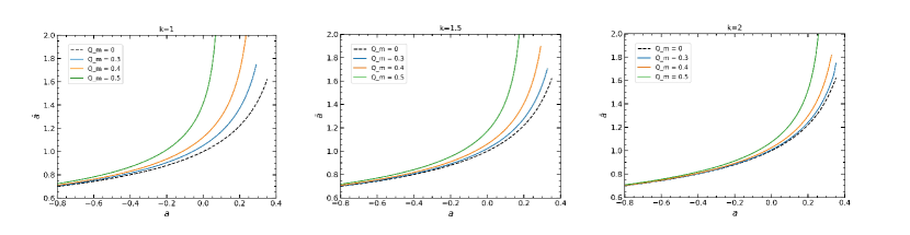
Figure 5: The variations of the lens coefficient $\bar{a}$ with respect to the spin parameter $a$ and the short-hair parameter $Q_{m}$ for three models.

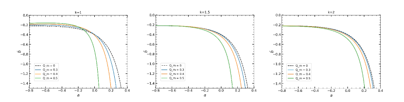
Figure 6: The variations of the lens coefficient $\bar{b}$ with respect to the spin parameter $a$ and the short-hair parameter $Q_{m}$ for three models.

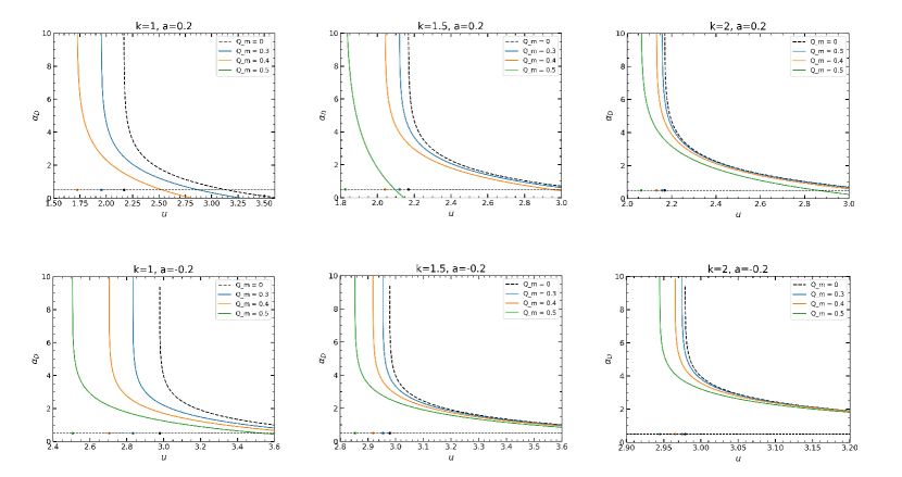
Figure 7: In the strong deflection limit, the deflection angle $\alpha_{D}$ of three rotating short-hairy BH models varies with the impact parameter $u$. From left to right, the models correspond to $k=1$, $k=1.5$, and $k=2$. From top to bottom, the spin parameters correspond to $a=-0.2$ and $a=0.2$.

IV Observational Effects of Strong Gravitational Lensing

IV.1 Lens Equation and Characteristic Observables

In gravitational lensing, if the positions of the lens and the light source are known, the specific positions of the images can be calculated using the lens equation. The lens equation is given in Virbhadra:1999nm , and later approximated using the small-angle approximation Bozza:2008ev ; Bozza:2001xd

$$\beta=\theta-\frac{D_{LS}}{D_{OS}}\Delta\alpha_{n}.$$ (41)

Here, $\beta$ represents the angle between the source and the lens axis, $\theta$ represents the angle between the image and the lens axis, $D_{LS}$ is the distance from the source to the lens, and $D_{OS}$ is the distance from the source to the observer. The relationship among the source, lens (black hole), and observer is given by $D_{OS}=D_{OL}+D_{LS}$. It is worth noting that, since the rotating short-hair black hole is asymptotically flat, for convenience of analysis, the source, lens, and observer can be set on the same line. In the above equation, $\Delta\alpha_{n}=\alpha(\theta)-2n\pi$ represents the remaining deflection angle after the light ray has looped around the black hole $n$ times.

To approximate the deflection $\Delta\alpha_{n}$, we use the analysis from Bozza:2002af . For the $n$-th image, the relationship is given by

$$\theta_{n}=\theta_{n}^{0}+\Delta\theta_{n},$$ (42)

where

$$\theta_{n}^{0}=\frac{u_{m}(1+e_{n})}{D_{OL}},$$ (43)

$$e_{n}=\exp\left(\frac{\bar{b}-2n\pi}{\bar{a}}\right),$$ (44)

$$\Delta\theta_{n}=\frac{D_{OS}}{D_{LS}}\frac{u_{m}e_{n}}{\bar{a}D_{OL}}(\beta-\theta_{n}^{0}).$$ (45)

Here, $\theta_{n}^{0}$ corresponds to the angle $\theta$ when $\alpha=2n\pi$. By combining these relationships, the approximate position of the $n$-th image can be obtained as Bozza:2002zj

$$\theta_{n}=\theta_{n}^{0}+\frac{u_{m}e_{n}(\beta-\theta_{n}^{0})D_{OS}}{\bar{a}D_{LS}D_{OL}}.$$ (46)

Note that the relativistic images obtained from equation (46) are only for the images on the same side. For the images on the other side, we can use $-\beta$ in a similar form. It is evident from equation (46) that the latter term is merely a correction to $\theta_{n}^{0}$. Clearly, when $\beta=\theta_{n}^{0}$, the $n$-th image is not corrected. Since our lens and source are on the same line, i.e., $\beta=0$, the expression for the Einstein ring can be obtained as Einstein:1936llh

$$\theta_{n}^{E}=\left(1-\frac{u_{m}e_{n}D_{OS}}{\bar{a}D_{LS}D_{OL}}\right)\theta_{n}^{0}.$$ (47)

If we adopt a clever configuration where the lens (black hole) is situated midway between the observer and the source, then $D_{OS}=D_{LS}=2D_{OL}$. Given that $D_{OL}$ is much larger than the impact parameter $b_{m}$, when $n=1$, the above expression can be approximated as

$$\theta_{1}^{E}\approx\frac{(1+e_{1})u_{m}}{D_{OL}},$$ (48)

where $e_{1}=\exp\left(\frac{\bar{b}-2\pi}{\bar{a}}\right)$.

Of course, in a lensing system, in addition to the corresponding angular position, the magnification is also an important observable quantity. The magnification of the $n$-th image can be expressed as Bozza:2002zj ; Virbhadra:1998dy ; Virbhadra:2007kw

$$\mu_{n}=\left(\frac{\beta}{\theta}\frac{d\beta}{d\theta}\right)^{-1}\Bigg{|}_{\theta_{n}^{0}}=\frac{u_{m}^{2}(1+e_{n})D_{OS}}{\bar{a}\beta D_{LS}D_{OL}^{2}}e_{n}.$$ (49)

It is evident from the above expression that due to the presence of the $e_{n}$ term, the magnification of the image decreases exponentially with increasing $n$. Additionally, when $\beta$ is very small and approaches zero, we can obtain relatively bright images. In other words, images are easier to observe when $\beta\to 0$. Clearly, the magnification is largest when $n=1$, meaning the image is the brightest at this point. Therefore, if we resolve the first-order image $\theta_{1}$ (the dominant image) and represent the other unresolved images as $\theta_{\infty}$, we can obtain several interesting observables Bozza:2002zj

$$\theta_{\infty}=\frac{u_{m}}{D_{OL}},$$ (50)

$$S=\theta_{1}-\theta_{\infty}=\theta_{\infty}\exp\left(\frac{\bar{b}-2\pi}{\bar{a}}\right),$$ (51)

$$r_{\text{mag}}=\frac{\mu_{1}}{\sum_{n=2}^{\infty}\mu_{n}}\approx\frac{5\pi}{\bar{a}\ln(10)}.$$ (52)

Here, $\theta_{\infty}$ represents the angular position of the unresolved bundled images, $s$ denotes the angular separation between the first resolved image (the outermost image) and the bundled images, and $r_{\text{mag}}$ is the brightness ratio between the outermost image and the remaining bundled images. These observables will be interesting and are discussed in detail in Section IV.2.

In addition to the observational effects mentioned above, time delay is also an important physical quantity. In the study of gravitational lensing effects, when light passes by a BH, its path bends due to gravity, forming multiple images. These images, because of different light paths, reach the observer at different times, which is known as time delay. This phenomenon can be used to determine the geometric scale and mass of the lensing system in observations and to estimate the Hubble constant in a cosmological context Birrer:2022chj ; Treu:2022aqp ; Grillo:2018ume . Here, we use the method proposed by Bozza and Mancini for calculating time delay in the strong field limit Bozza:2003cp . For a lensing system aligned on a straight line ($\beta=0$) and two relativistic images on the same side of the lens (the $p$-th and $q$-th images), the time delay formula is given by Bozza:2003cp

$$\Delta T_{p,q}=2\pi(p-q)\frac{\tilde{a}}{\bar{a}}+2\sqrt{\frac{A_{m}u_{m}}{B_{m}}}\sqrt{u_{m}}\left(e^{-\frac{\bar{b}-2p\pi}{2\bar{a}}}-e^{-\frac{\bar{b}-2q\pi}{2\bar{a}}}\right).$$ (53)

Analyzing the above equation, the first term represents the geometric time delay, which mainly depends on the number of loops the light makes around the black hole. The second term represents the time dilation effect of the light in the gravitational field. It is evident that the time delay is primarily determined by the difference in the number of loops the light makes around the BH, so the dominant term is the first term. Thus, the above equation can be approximated as

$$\Delta T_{p,q}\approx 2\pi(p-q)\frac{\tilde{a}}{\bar{a}}=2\pi(p-q)u_{m}=2\pi(p-q)\theta_{\infty}D_{OL}.$$ (54)

Above, we have presented many interesting observables, such as the Einstein ring, three notable observables, and time delay. With these expressions, we can evaluate the lensing observables in the real universe. In Section IV.2, we will take the supermassive BHs $M87^{*}$ and $SgrA^{*}$ as observational targets to evaluate the lensing observables in the real universe.

IV.2 Evaluating the Observability of Supermassive Black Holes

In this subsection, we will consider the rotating short-hairy BH, which is closer to those existing in the real universe, as candidates for the supermassive BHs $M87^{*}$ and $SgrA^{*}$ in the universe. This will allow us to study their corresponding observables. For the supermassive BH $M87^{*}$ in the universe, the latest astronomical observations show that the mass of $M87^{*}$ is $(6.5\pm 0.7)\times 10^{9}M_{\odot}$, and its distance from Earth is $(16.8\pm 0.8)$ Mpc EventHorizonTelescope:2019ggy . For the supermassive BH $SgrA^{*}$, its mass is $3.98\times 10^{6}M_{\odot}$, and its distance is $7.97$ kpc Chen:2019tdb . By considering rotating short-hairy BH as candidates for these two supermassive BHs, we can indirectly obtain the corresponding information ($D_{OL}$ and $M$). With this information, we can evaluate the observables calculated in the previous subsection.

We first evaluate the Einstein rings for the supermassive BHs $M87^{*}$ and $SgrA^{*}$. From the magnification, it is known that the magnification of the first image layer is much higher than that of the other image layers. This is because the magnification decreases exponentially with the increase in the number of relativistic image layers (see equation 49). Therefore, it is more meaningful to plot the Einstein ring of the first layer. Here, we use the expressions given in Section IV.1 to plot the Einstein rings for the respective BHs. As shown in Figure 8, when the rotating short-hairy BH degenerates to a non-rotating case ($a=0$), the size of the Einstein ring decreases with the increase of short-hair parameter, where the dashed line represents the Einstein ring for a supermassive BH treated as a Schwarzschild BH. Clearly, the presence of hair $Q_{m}$ affects the Einstein ring, but these effects are minor and difficult to distinguish at the current level of observation. Meanwhile, comparing the first and second figures of Figure 8, it is found that the Einstein ring of the $SgrA^{*}$ BH is larger than that of the $M87^{*}$ BH under the same conditions. This phenomenon is because the $SgrA^{*}$ BH is closer to Earth than the $M87^{*}$ BH, so the Einstein ring presented by the $SgrA^{*}$ BH as a lens is naturally larger than that of the $M87^{*}$ BH. Regarding the impact of parameter $k$, as shown in the figure, the Einstein ring gradually increases as the parameter $k$ increases. However, it is easy to see that if the parameter $k$ is very large, the Einstein rings of the short-hairy BH and the Schwarzschild BH will degenerate, making it even more difficult to distinguish them. In other words, to effectively observe these differences in the future, it is necessary to limit the parameter $k$ to small values to make the differences more easily discernible.

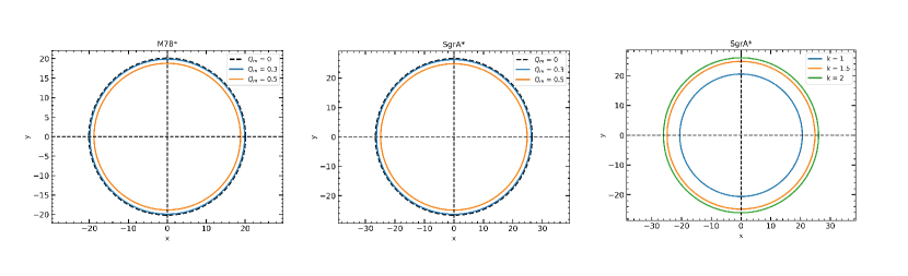
Figure 8: In the context of the Einstein rings for the BHs $M87^{*}$ and $SgrA^{*}$, the first two images correspond to the Einstein rings of$M87^{*}$ and $M87^{*}$ under conditions where $a=0$ and $k=1.5$. The third image represents the Einstein ring of $M87^{*}$ with parameters $a=0$ and $Q_{m}=0.5$

For three intriguing observations, when treating the rotating short-hairy BH as the corresponding supermassive BHs ($M87^{*}$ and $SgrA^{*}$), as shown in Figure 9, we numerically calculated the corresponding relativistic image $\theta_{\infty}$, angular distance $S$, and image magnification $r_{mag}$. Evidently, the trend of observational changes is the same for both $SgrA^{*}$ and $M87^{*}$ BHs. Specifically, the relativistic image $\theta_{\infty}$ decreases with increasing spin parameter $a$ and short-hair parameter $Q_{m}$, while the angular distance $S$ increases, and the magnification $r_{mag}$ decreases. Furthermore, due to the presence of the short-hair parameter, the increasing trends become more pronounced, as do the decreasing trends. Additionally, it is easy to observe from the figure that if the parameter $k$ takes a larger value, the influence of the short-hair parameter $Q_{m}$ will degenerate to the standard Kerr BH scenario (the dashed line in Figure 9 represents the Kerr BH). Combining Tables 1 to 3 and Figure 9, it is evident that for the $M87^{*}$ BH, the maximum variation in the angular position of the relativistic image due to the short-hair parameter $Q_{m}$ is within the range of $20.1042\,\mu as>\theta_{\infty}(M87^{*})>14.1238\,\mu as$, which falls within the range of the EHT’s observations of the supermassive $M87^{*}$ BH diameter ($42\pm 3\,\mu as$) EventHorizonTelescope:2019dse . For the $SgrA^{*}$ BH, the range affected by the short-hair parameter is $25.9482\,\mu as>\theta_{\infty}(SgrA^{*})>18.2294\,\mu as$, which is comparable to the EHT’s observations of the supermassive $SgrA^{*}$ BH’s shadow diameter ($51.8\pm 2.3\,\mu as$) EventHorizonTelescope:2022wkp . Clearly, the observational ranges for both BHs are on the order of $\mu as$, which aligns with the current capabilities of the EHT. However, it is regrettable that these deviations cannot be detected by existing equipment. From Tables 4 to 6, it can be seen that under the same conditions (same spin parameter), when considering the rotating short-hairy BH as a supermassive $M87^{*}$ BH, the deviation in the angular position of the relativistic image due to the short-hair parameter $Q_{m}$ is less than $5\,\mu as$, and the maximum deviation in the angular separation between the first image and other images is below $0.13\,\mu as$. For the supermassive $SgrA^{*}$ BH, the deviation in the angular position is below $6\,\mu as$, and the maximum deviation in angular separation between images is less than $0.17\,\mu as$. These differences, although on the order of $\mu as$ (especially in angular position), cannot be distinguished by the current angular resolution of the EHT, which is approximately $20\,\mu as$ EventHorizonTelescope:2019ths . This means that distinguishing these differences to test the no-hair theorem might require waiting for the next generation of the EHT. This presents a promising future because, once these differences can be discerned, it would not only allow us to distinguish rotating short-hairy BH from Kerr BH but also provide further insights into the properties of the short-hair parameter $Q_{m}$, indirectly testing the no-hair theorem.

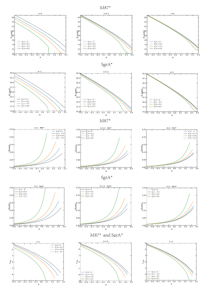
Figure 9: The three observational values in the $M87^{*}$ and $SgrA^{*}$ BHs vary with the spin parameter, with the corresponding parameter values indicated in the chart.

		$M87^{*}$			$SgrA^{*}$			$M87^{*}$	$SgrA^{*}$	Lensing Coefficients
$a$	$Q_{m}$	$\theta_{\infty}(\mu as)$	$S(\mu as)$	$r_{mag}$	$\theta_{\infty}(\mu as)$	$S(\mu as)$	$r_{mag}$	$\Delta T_{21}(h)$	$\Delta T_{21}(min)$	$\bar{a}$	$\bar{b}$
-0.2	0	23.0501	0.0132	7.7554	29.7505	0.0171	7.7554	337.0617	12.3831	0.8796	-0.281
	0.3	21.9225	0.0159	7.5398	28.2951	0.0205	7.5398	320.5724	11.7773	0.9048	-0.257
	0.4	20.9262	0.0196	7.2929	27.0091	0.0253	7.2929	306.0031	11.2421	0.9354	-0.2382
	0.5	19.3868	0.0314	6.72	25.0223	0.0406	6.72	283.4932	10.4151	1.0152	-0.2388
0	0	20.1042	0.0252	6.8219	25.9482	0.0325	6.8219	293.9829	10.8005	1	-0.4002
	0.1	19.9691	0.0258	6.7909	25.7738	0.0333	6.7909	292.0076	10.7279	1.0046	-0.3993
	0.2	19.5502	0.0279	6.6898	25.2332	0.036	6.6898	285.8825	10.5029	1.0197	-0.3972
	0.3	18.7985	0.0328	6.4857	24.263	0.0424	6.4857	274.8906	10.0991	1.0518	-0.3965
	0.4	17.5886	0.0453	6.0738	22.7014	0.0584	6.0738	257.1985	9.4491	1.1232	-0.4136
	0.5	15.4762	0.1084	4.8238	19.9749	0.1399	4.8238	226.3082	8.3142	1.4142	-0.7332
0.2	0	16.7805	0.052	5.5874	21.6584	0.0671	5.5874	245.3812	9.0149	1.2209	-0.77
	0.3	15.1153	0.0776	4.9733	19.5091	0.1001	4.9733	221.031	8.1203	1.3717	-0.9488
	0.4	13.3343	0.1342	4.0314	17.2104	0.1732	4.0314	194.9873	7.1635	1.6922	-1.4988
	0.5

Table 1: When considering the $M87^{*}$ and $SgrA^{*}$ BHs as rotating short-hairy BH with $k=1$, the observational values and lensing coefficients corresponding to different short-hair parameters $Q_{m}$ are evaluated, as well as the time delay under different parameters. When $a=0$ and $Q_{m}\neq 0$, the rotating short-hairy BH becomes a Reissner-Nordström BH.

		$M87^{*}$			$SgrA^{*}$			$M87^{*}$	$SgrA^{*}$	Lensing Coefficients
$a$	$Q_{m}$	$\theta_{\infty}(\mu as)$	$S(\mu as)$	$r_{mag}$	$\theta_{\infty}(\mu as)$	$S(\mu as)$	$r_{mag}$	$\Delta T_{21}(h)$	$\Delta T_{21}(min)$	$\bar{a}$	$\bar{b}$
-0.2	0	23.0501	0.0132	7.7554	29.7505	0.0171	7.7554	337.0617	12.3831	0.8796	-0.281
	0.3	22.8603	0.0144	7.6559	29.5055	0.0186	7.6559	334.2858	12.2811	0.8911	-0.2824
	0.4	22.5845	0.0165	7.498	29.1495	0.0213	7.498	330.2524	12.133	0.9098	-0.2875
	0.5	22.0792	0.0218	7.1564	28.4973	0.0282	7.1562	322.8638	11.8615	0.9533	-0.3123
0	0	20.1042	0.0252	6.8219	25.9482	0.0325	6.8219	293.9829	10.8005	1	-0.4002
	0.3	19.8547	0.0284	6.675	25.6262	0.0366	6.675	290.335	10.6665	1.022	-0.4124
	0.4	19.4815	0.0344	6.43	25.1445	0.0445	6.43	284.8777	10.466	1.0609	-0.4408
	0.5	18.7497	0.0541	5.8239	24.2001	0.0698	5.8239	274.1775	10.0729	1.1714	-0.5677
0.2	0	16.7805	0.052	5.5874	21.6584	0.0671	5.5874	245.3812	9.0149	1.2209	-0.77
	0.3	16.4046	0.0624	5.3286	21.1732	0.0805	5.3286	239.8844	8.813	1.2802	-0.8508
	0.4	15.7954	0.0861	4.8396	20.3869	0.1111	4.8396	230.976	8.4857	1.4096	-1.0636
	0.5	14.1238	0.1811	2.265	18.2294	0.2337	2.265	206.5317	7.5877	3.0119	-6.8386

Table 2: When considering the $M87^{*}$ and $SgrA^{*}$ BHs as rotating short-hairy BH with $k=1.5$, we evaluate the observational values, lensing coefficients, and time delays corresponding to different short-hair parameters $Q_{m}$.

		$M87^{*}$			$SgrA^{*}$			$M87^{*}$	$SgrA^{*}$	Lensing Coefficients
$a$	$Q_{m}$	$\theta_{\infty}(\mu as)$	$S(\mu as)$	$r_{mag}$	$\theta_{\infty}(\mu as)$	$S(\mu as)$	$r_{mag}$	$\Delta T_{21}(h)$	$\Delta T_{21}(min)$	$\bar{a}$	$\bar{b}$
-0.2	0	23.0501	0.0132	7.7554	29.7505	0.0171	7.7554	337.0617	12.3831	0.8796	-0.281
	0.3	23.0175	0.0136	7.7234	29.7083	0.0175	7.7234	336.5843	12.3656	0.8833	-0.2838
	0.4	22.9454	0.0144	7.6505	29.6153	0.0186	7.6505	335.53	12.3269	0.8917	-0.2907
	0.5	22.7856	0.0165	7.4776	29.4091	0.0214	7.4776	333.1942	12.241	0.9123	-0.3106
0	0	20.1042	0.0252	6.8219	25.9482	0.0325	6.8219	293.9829	10.8005	1	-0.4002
	0.3	20.0554	0.0262	6.7716	25.8852	0.0338	6.7716	293.2696	10.7743	1.0074	-0.408
	0.4	19.9461	0.0286	6.6543	25.7442	0.037	6.6543	291.6718	10.7156	1.0252	-0.4279
	0.5	19.695	0.0357	6.3557	25.4201	0.0461	6.3557	288.0004	10.5807	1.0733	-0.4919
0.2	0	16.7805	0.052	5.5874	21.6584	0.0671	5.5874	245.3812	9.0149	1.2209	-0.77
	0.3	16.6933	0.0555	5.4914	21.5458	0.0717	5.4914	244.1059	8.9681	1.2423	-0.8051
	0.4	16.4898	0.0651	5.2522	21.2832	0.084	5.2522	241.1305	8.8588	1.2989	-0.906
	0.5	15.9585	0.1017	4.4866	20.5974	0.1312	4.4866	233.3603	8.5733	1.5205	-1.4047

Table 3: When considering the $M87^{*}$ and $SgrA^{*}$ BHs as rotating short-hairy BH with $k=2$, we evaluate the observational values, lensing coefficients, and time delays corresponding to different short-hair parameters $Q_{m}$.

		$M87^{*}$			$SgrA^{*}$			$M87^{*}$	$SgrA^{*}$
$a$	$\delta Q_{m}$	$\delta\theta_{\infty}(\mu as)$	$\delta S(\mu as)$	$\delta r_{mag}$	$\delta\theta_{\infty}(\mu as)$	$\delta S(\mu as)$	$\delta r_{mag}$	$\delta\Delta T_{21}(h)$	$\delta\Delta T_{21}(min)$
-0.2	0.3	-1.1276	0.0027	-0.2156	-1.4554	0.0034	-0.2156	-16.4893	-0.6058
	0.4	-2.1239	0.0064	-0.4625	-2.7414	0.0082	-0.4625	-31.0586	-1.141
	0.5	-3.6633	0.0182	-1.0354	-4.7282	0.0235	-1.0354	-53.5685	-1.968
	0.3	-1.3057	0.0076	-0.3362	-1.6852	0.0099	-0.3362	-19.0923	-0.7014
	0.4	-2.5156	0.0201	-0.7481	-3.2468	0.0259	-0.7481	-36.7844	-1.3514
	0.5	-4.628	0.0832	-1.9981	-5.9733	0.1074	-1.9981	-67.6747	-2.4863
0.2	0.3	-1.6652	0.0256	-0.6141	-2.1493	0.033	-0.6141	-24.3502	-0.8946
	0.4	-3.4462	0.0822	-1.556	-4.448	0.1061	-1.556	-50.3939	-1.8514
	0.5

Table 4: The deviation between the rotating short-hairy BH and the Kerr BH is represented as $\delta(W)=W_{\text{hairy}}-W_{\text{Kerr}}$, where the Kerr BH corresponds to the case with a short-hair parameter $Q_{m}=0$. When $a=0$ and $Q_{m}=0$, the BH becomes a Reissner-Nordström BH. When $a=0$ and $Q_{m}\neq 0$, it represents a Schwarzschild-like BH with hair. Here, $k=1$.

		$M87^{*}$			$SgrA^{*}$			$M87^{*}$	$SgrA^{*}$
$a$	$\delta Q_{m}$	$\delta\theta_{\infty}(\mu as)$	$\delta S(\mu as)$	$\delta r_{mag}$	$\delta\theta_{\infty}(\mu as)$	$\delta S(\mu as)$	$\delta r_{mag}$	$\delta\Delta T_{21}(h)$	$\delta\Delta T_{21}(min)$
-0.2	0.3	-0.1898	0.0012	-0.0995	-0.245	0.0015	-0.0995	-2.7759	-0.102
	0.4	-0.4656	0.0033	-0.2574	-0.601	0.0042	-0.2574	-6.8093	-0.2501
	0.5	-0.9709	0.0086	-0.599	-1.2532	0.0111	-0.5992	-14.1979	-0.5216
0	0.3	-0.2495	0.0032	-0.1469	-0.322	0.0041	-0.1469	-3.6479	-0.134
	0.4	-0.6227	0.0092	-0.3919	-0.8037	0.012	-0.3919	-9.1052	-0.3345
	0.5	-1.3545	0.0289	-0.998	-1.7481	0.0373	-0.998	-19.8054	-0.7276
0.2	0.3	-0.3759	0.0104	-0.2588	-0.4852	0.0134	-0.2588	-5.4968	-0.2019
	0.4	-0.9851	0.0341	-0.7478	-1.2715	0.044	-0.7478	-14.4052	-0.5292
	0.5	-2.6567	0.1291	-3.3224	-3.429	0.1666	-3.3224	-38.8495	-1.4272

Table 5: At $k=1.5$, the deviation of the corresponding observational values from those of a Kerr BH or a Schwarzschild BH is given by $\delta(W)=W_{\text{hairy}}-W_{\text{Kerr}}$. When $a=0$ and $Q_{m}=0$, the rotating short-hairy BH becomes a Schwarzschild BH. When $a\neq 0$ and $Q_{m}=0$, the rotating short-hairy BH reduces to a Kerr BH.

		$M87^{*}$			$SgrA^{*}$			$M87^{*}$	$SgrA^{*}$
$a$	$\delta Q_{m}$	$\delta\theta_{\infty}(\mu as)$	$\delta S(\mu as)$	$\delta r_{mag}$	$\delta\theta_{\infty}(\mu as)$	$\delta S(\mu as)$	$\delta r_{mag}$	$\delta\Delta T_{21}(h)$	$\delta\Delta T_{21}(min)$
-0.2	0.3	-0.0326	0.0004	-0.032	-0.0422	0.0004	-0.032	-0.4774	-0.0175
	0.4	-0.1047	0.0012	-0.1049	-0.1352	0.0015	-0.1049	-1.5317	-0.0562
	0.5	-0.2645	0.0033	-0.2778	-0.3414	0.0043	-0.2778	-3.8675	-0.1421
0	0.3	-0.0488	0.001	-0.0503	-0.063	0.0013	-0.0503	-0.7133	-0.0262
	0.4	-0.1581	0.0034	-0.1676	-0.204	0.0045	-0.1676	-2.3111	-0.0849
	0.5	-0.4092	0.0105	-0.4662	-0.5281	0.0136	-0.4662	-5.9825	-0.2198
0.2	0.3	-0.0872	0.0035	-0.096	-0.1126	0.0046	-0.096	-1.2753	-0.0468
	0.4	-0.2907	0.0131	-0.3352	-0.3752	0.0169	-0.3352	-4.2507	-0.1561
	0.5	-0.822	0.0497	-1.1008	-1.061	0.0641	-1.1008	-12.0209	-0.4416

Table 6: For $k=2$, the deviation of the corresponding observational values from those of a Kerr BH or a Schwarzschild BH is given by $\delta(W)=W_{\text{hairy}}-W_{\text{Kerr}}$. When $a=0$ and $Q_{m}=0$, the rotating short-hairy BH becomes a Schwarzschild BH. When $a\neq 0$ and $Q_{m}=0$, the rotating short-hairy BH reduces to a Kerr BH.

For two relativistic images located on the same side of a BH, the time delay between the second relativistic image ($p=2$) and the first relativistic image ($q=1$) is shown in Tables 1 to 3, and the deviation values are presented in Tables 4 to 6. Here, we consider the time delay primarily determined by the optical path difference between relativistic images formed after the light circles the BH multiple times (see Figure 7, where the light path clearly wraps around more than $2\pi$ near the divergence of the deflection angle). When considering the $M87^{*}$ and $SgrA^{*}$ BH as rotating short-hairy BH, the time delay $\Delta T_{2,1}$ between the second and first relativistic images on the same side can be as high as $293.98$ hours for the former and up to $10.8$ minutes for the latter. Clearly, the time delay for the former is sufficient for astronomical observation, providing the necessary conditions for exploring the properties of rotating short-hairy BH (see Tables 1 to 3). In the same conditions, the time delay deviation between rotating short-hairy BH and Kerr BH, with the $SgrA^{*}$ BH as the background, can reach a relative deviation of up to $2.49$ minutes, while for the $M87^{*}$ BH, the relative deviation can be as high as $67.67$ hours. Overall, for the $SgrA^{*}$ BH, the time delay deviation is within a few minutes, making it challenging to detect in astronomy. However, for the $M87^{*}$ BH, the time delay deviation between rotating short-hairy BH and Kerr BH is within several hours or even days, making it feasible for astronomical observation. From the perspective of time delay alone, distinguishing between Kerr BH and rotating short-hairy BH in the $M87^{*}$ BH is feasible, provided that the equipment used is capable of resolving the two relativistic images. As discussed above, current equipment does not meet this requirement, but the next generation of EHT is expected to achieve such resolution. If these images can be resolved in the near future, it will yield significant physical information, such as testing the no-hair theorem, exploring the nature of the short-hair parameter $Q_{m}$, and constraining parameter variations.

V Discussion and conclusions

The strong gravitational lensing effect is especially important in astronomy, particularly in studying the physical properties of BHs and their surrounding environments. The intense gravitational field of a BH significantly bends light, creating multiple relativistic images, each with different imaging times. Through precise time-delay measurements, astronomers can accurately infer the mass distribution and spacetime structure of BHs, providing a unique perspective for studying the extreme physical environments of BHs. Gravitational lensing research has long been a significant topic, and it became even more popular after the successful imaging of the $M87^{*}$ BH in 2019. In the literature EventHorizonTelescope:2019dse , they observed that the diameter of the $M87^{*}$ BH shadow was consistent with the theoretical calculations for a Kerr BH, suggesting that BH in the real universe are likely similar to Kerr BH. However, BHs in reality do not exist in isolation but are surrounded by various types of matter, such as accretion disks, dark matter, and other forms of matter. This implies that the vacuum isolation model of a Kerr BH is not entirely applicable in the real universe. Therefore, it is necessary to consider other forms of Kerr-like BH as candidates for astrophysical BH. In particular,a rotating short-hairy BH, which consider additional short-hair and the anisotropy of matter, are more likely to exist in the real universe. Studying such a BH is more valuable because a rotating short-hairy BH can effectively include a Kerr BH (when $Q_{m}=0$, a rotating short-hairy BH reduces to a Kerr BH). By studying the lensing behavior of such a BH, one can not only distinguish a Kerr BH and test the no-hair theorem but also constrain the short-hair parameter and further explore its properties through lensing effects.

Based on these considerations, exploring the strong gravitational lensing behavior in rotating short-hairy BH is meaningful. In our study, the event horizon radius of a rotating short-hairy BH gradually decreases as the short-hair parameter increases. Under equivalent conditions, the presence of the short-hair parameter causes the event horizon radius to be smaller than that of a Kerr BH. As the parameter $k$ increases, the event horizon radius of the rotating short-hairy BH approaches that of the Kerr BH and eventually coincides, forming a degenerate situation (as shown in Figure 1). Similarly, the photon sphere and impact parameter decrease monotonically with the increase of the BH’s spin parameter. Under the same conditions, the photon sphere radius or impact parameter of a Kerr BH is greater than that of a rotating short-hairy BH, and the stronger the short-hair parameter, the greater the deviation. As the parameter $k$ increases, the photon sphere or impact parameter also approaches the Kerr BH and eventually becomes degenerate (as shown in Figures 3 and 4). For the lensing coefficients $\bar{a}$ and $\bar{b}$, the trends are opposite as the BH spin parameter changes: the former increases monotonically, while the latter decreases monotonically. The presence of the short-hair causes the increasing ones to grow faster and the decreasing ones to shrink faster (as shown in Figures 5 and 6). Interestingly, the short-hair parameter $Q_{m}$ can cause the lensing coefficient $\bar{b}$ to be higher to some extent than that of Kerr black holes. As can be clearly seen in Figure 6, in certain situations, the influence of the hair parameter $Q_{m}$ results in the lensing coefficient $\bar{b}$ exceeding that of the Kerr BH. Regarding the deflection angle $\alpha_{D}$, it gradually decreases as the impact parameter increases. When the deflection angle decreases below zero, the strong field limit no longer applies. At the impact parameter $u=u_{m}$, the deflection angle $\alpha_{D}$ diverges, and the impact parameter divergence for a rotating short-hairy BH is generally smaller than that of a Kerr BH (the black dashed line in the figure represents the Kerr BH). However, near $u_{m}$, the deflection angle is greater than $2\pi$, meaning that the light circles the BH once or multiple times, providing conditions for the formation of relativistic images (as shown in Figure 7).

Considering rotating short-hairy BH as supermassive $M87^{*}$ and $SgrA^{*}$ BHs allows us to analyze the corresponding observational quantities. Regarding the Einstein ring, for both $M87^{*}$ and $SgrA^{*}$ BHs, the presence of the short-hair parameter makes the Einstein ring smaller than that of a BH without hair. As the parameter $k$ increases, the Einstein ring also gradually increases, but eventually, a degenerate situation occurs (as shown in Figure 8). This is further corroborated by changes in the angular position of the lensing observational values, as shown in Figure 9, where the presence of the hair parameter results in angular positions smaller than those under a Kerr BH in the same conditions. For the three observational quantities, regardless of whether it is the $M87^{*}$ BH or the $SgrA^{*}$ BH, the trends are consistent: the relativistic image $\theta_{\infty}$ decreases with increasing spin parameter, the angular distance $S$ increases with increasing spin parameter, and the relativistic image magnification $r_{mag}$ decreases with increasing spin parameter. The presence of short-hair causes $\theta_{\infty}$ and $s$ to be smaller than those of a Kerr BH, while $r_{mag}$ is larger. The stronger the short-hair intensity, the greater the deviation. The short-hair parameter $Q_{m}$ has a maximum impact range on the angular position of the relativistic image as follows: $20.1041\,\mu as>\theta_{\infty}\,(M87^{*})>14.1238\,\mu as$ and $25.9482\,\mu as>\theta_{\infty}\,(SgrA^{*})>18.2294\,\mu as$. These ranges are comparable to the shadow diameters observed by the EHT for $M87^{*}$ and $SgrA^{*}$ BHs EventHorizonTelescope:2019dse ; EventHorizonTelescope:2022xqj (as shown in Figure 9 and Tables 1 to 3). We also discuss the time delay between the second and first relativistic images on the same side of the lens. In the simulated $SgrA^{*}$ BH, the time delay $\Delta T_{2,1}$ between the two relativistic images reaches several minutes. In the simulated $M87^{*}$ BH, the time delay $\Delta T_{2,1}$ can be as high as several hundred hours. The former duration is insufficient for astronomical measurement, but the latter is adequate for astronomical observation. Simultaneously, we obtained some deviation values ($\delta(W)=W_{\text{hairy}}-W_{\text{Kerr}}$). As shown in Tables 4 to 6, it is evident that when considering rotating short-hairy BH as supermassive $M87^{*}$ or $SgrA^{*}$ BHs, for the former, the angular position deviation from a Kerr BH is less than $5\,\mu as$, and the angular separation deviation is less than $0.13\,\mu as$. The angular separation between the two relativistic images is greater than that of a Kerr BH, and the time delay $\Delta T_{2,1}$ deviation from a Kerr BH $\delta\Delta T_{2,1}$ can be as much as tens of hours. For the latter, the angular position deviation is less than $6\,\mu as$, and the angular separation deviation is less than $0.17\,\mu as$. Similarly, the angular separation is greater than that of a Kerr BH under the same conditions, and the time delay deviation $\delta\Delta T_{2,1}$ is within a few minutes. It is clear that treating rotating short-hairy BH as $M87^{*}$ BH makes it easier to distinguish them from Kerr BH.

In conclusion, when considering rotating short-hairy BH as supermassive $M87^{*}$ and $SgrA^{*}$ BHs, numerical simulations reveal significant differences between rotating short-hairy BH and Kerr BH. However, these differences, while consistent with the current observational capabilities of the EHT, unfortunately, cannot be distinguished by the precision of existing equipment. Therefore, to truly differentiate between rotating short-hairy BH and Kerr BH and thereby test the no-hair theorem, we may need to wait for the next generation of the EHT. This promises a promising future because, once the next-generation EHT can distinguish these differences, we will not only be able to separate rotating short-hairy BH from Kerr BH but also gain further insight into the properties of the short-hair parameter $Q_{m}$, indirectly testing the no-hair theorem. It is worth mentioning that in our analysis, we found an interesting phenomenon: when the parameter $k$ is relatively large, the rotating short-hairy BH and Kerr BH become degenerate, and all physical behaviors coincide with those of Kerr BH, making it more difficult to distinguish between rotating short-hairy BH and Kerr BH. Therefore, regarding parameter constraints, we provided a preliminary discussion, suggesting that the value of the parameter $k$ should not be too large (values of $1$, $1.5$, and $2$ are more suitable), as excessively large values lead to indistinguishable differences (degeneracy phenomenon). Similarly, the strength of the short-hair parameter $Q_{m}$ cannot be infinitely large due to the limitations of the BH event horizon and the observational range of the EHT. In the future, through the observation of BH shadows by the EHT, we will be able to determine more specific constraints. We plan to use these observational results to provide parameter constraints within the first confidence interval. Additionally, studying weak gravitational lensing effects will be the focus of our subsequent work, which will help us gain a deeper understanding of the properties of rotating short-hairy BH.

VI acknowledgements

We acknowledge the anonymous referee for a constructive report that has significantly improved this paper. This work was supported by the Special Natural Science Fund of Guizhou University (Grant No.X2022133), the National Natural Science Foundation of China (Grant No. 12365008) and the Guizhou Provincial Basic Research Program (Natural Science) (Grant No. QianKeHeJiChu-ZK[2024]YiBan027) .

References

- (1) B. P. Abbott et al. GW150914: The Advanced LIGO Detectors in the Era of First Discoveries. Phys. Rev. Lett., 116(13):131103, 2016.
- (2) Saul A. Teukolsky. The Kerr Metric. Class. Quant. Grav., 32(12):124006, 2015.
- (3) Jiahao Tao, Shafqat Riaz, Biao Zhou, Askar B. Abdikamalov, Cosimo Bambi, and Daniele Malafarina. Testing the -Kerr metric with black hole x-ray data. Phys. Rev. D, 108(8):083036, 2023.
- (4) Mustapha Azreg-Aïnou. Generating rotating regular black hole solutions without complexification. Phys. Rev. D, 90(6):064041, 2014.
- (5) Sushant G. Ghosh. A nonsingular rotating black hole. Eur. Phys. J. C, 75(11):532, 2015.
- (6) Zhaoyi Xu, Jiancheng Wang, and Meirong Tang. Deformed black hole immersed in dark matter spike. JCAP, 09:007, 2021.
- (7) J. David Brown and Viqar Husain. Black holes with short hair. Int. J. Mod. Phys. D, 6:563–573, 1997.
- (8) S. W. Hawking. Black holes in general relativity. Commun. Math. Phys., 25:152–166, 1972.
- (9) Werner Israel. Event horizons in static vacuum space-times. Phys. Rev., 164:1776–1779, 1967.
- (10) Bum-Hoon Lee, Wonwoo Lee, and Daeho Ro. Expanded evasion of the black hole no-hair theorem in dilatonic Einstein-Gauss-Bonnet theory. Phys. Rev. D, 99(2):024002, 2019.
- (11) Brian R. Greene, Samir D. Mathur, and Christopher M. O’Neill. Eluding the no hair conjecture: Black holes in spontaneously broken gauge theories. Phys. Rev. D, 47:2242–2259, 1993.
- (12) P. Bizon. Colored black holes. Phys. Rev. Lett., 64:2844–2847, 1990.
- (13) J. Ovalle, R. Casadio, E. Contreras, and A. Sotomayor. Hairy black holes by gravitational decoupling. Phys. Dark Univ., 31:100744, 2021.
- (14) Meirong Tang and Zhaoyi Xu. The no-hair theorem and black hole shadows. JHEP, 12:125, 2022.
- (15) Sidney Liebes. Gravitational Lenses. Phys. Rev., 133:B835–B844, 1964.
- (16) Yannick Mellier. Probing the universe with weak lensing. Ann. Rev. Astron. Astrophys., 37:127–189, 1999.
- (17) Jacek Guzik, Bhuvnesh Jain, and Masahiro Takada. Tests of Gravity from Imaging and Spectroscopic Surveys. Phys. Rev. D, 81:023503, 2010.
- (18) Fabian Schmidt. Weak Lensing Probes of Modified Gravity. Phys. Rev. D, 78:043002, 2008.
- (19) Richard Massey, Thomas Kitching, and Johan Richard. The dark matter of gravitational lensing. Rept. Prog. Phys., 73:086901, 2010.
- (20) S. Vegetti et al. Strong gravitational lensing as a probe of dark matter. 6 2023.
- (21) Ana Diaz Rivero and Cora Dvorkin. Direct Detection of Dark Matter Substructure in Strong Lens Images with Convolutional Neural Networks. Phys. Rev. D, 101(2):023515, 2020.
- (22) Atınç Çağan Şengül and Cora Dvorkin. Probing dark matter with strong gravitational lensing through an effective density slope. Mon. Not. Roy. Astron. Soc., 516(1):336–357, 2022.
- (23) Malcolm Fairbairn, Juan Urrutia, and Ville Vaskonen. Microlensing of gravitational waves by dark matter structures. JCAP, 07:007, 2023.
- (24) Lai Zhao, Meirong Tang, and Zhaoyi Xu. The Lensing Effect of Quantum-Corrected Black Hole and Parameter Constraints from EHT Observations. 3 2024.
- (25) Jacob D. Bekenstein and Robert H. Sanders. Gravitational lenses and unconventional gravity theories. Astrophys. J., 429:480, 1994.
- (26) Shafqat Ul Islam, Rahul Kumar, and Sushant G. Ghosh. Gravitational lensing by black holes in the Einstein-Gauss-Bonnet gravity. JCAP, 09:030, 2020.
- (27) Rahul Kumar, Shafqat Ul Islam, and Sushant G. Ghosh. Gravitational lensing by charged black hole in regularized Einstein–Gauss–Bonnet gravity. Eur. Phys. J. C, 80(12):1128, 2020.
- (28) Song-bai Chen and Ji-liang Jing. Strong field gravitational lensing in the deformed Hořava-Lifshitz black hole. Phys. Rev. D, 80:024036, 2009.
- (29) Samuel E. Gralla, Daniel E. Holz, and Robert M. Wald. Black Hole Shadows, Photon Rings, and Lensing Rings. Phys. Rev. D, 100(2):024018, 2019.
- (30) Valerio Bozza. Gravitational Lensing by Black Holes. Gen. Rel. Grav., 42:2269–2300, 2010.
- (31) V. Bozza, S. Capozziello, G. Iovane, and G. Scarpetta. Strong field limit of black hole gravitational lensing. Gen. Rel. Grav., 33:1535–1548, 2001.
- (32) V. Bozza. Quasiequatorial gravitational lensing by spinning black holes in the strong field limit. Phys. Rev. D, 67:103006, 2003.
- (33) K. S. Virbhadra and George F. R. Ellis. Schwarzschild black hole lensing. Phys. Rev. D, 62:084003, 2000.
- (34) V. Bozza. Gravitational lensing in the strong field limit. Phys. Rev. D, 66:103001, 2002.
- (35) Naoki Tsukamoto. Deflection angle in the strong deflection limit in a general asymptotically flat, static, spherically symmetric spacetime. Phys. Rev. D, 95(6):064035, 2017.
- (36) Jingyun Man and Hongbo Cheng. Analytical discussion on strong gravitational lensing for a massive source with a f(R) global monopole. Phys. Rev. D, 92(2):024004, 2015.
- (37) Shao-Wen Wei, Ke Yang, and Yu-Xiao Liu. Black hole solution and strong gravitational lensing in Eddington-inspired Born–Infeld gravity. Eur. Phys. J. C, 75:253, 2015. [Erratum: Eur.Phys.J.C 75, 331 (2015)].
- (38) Ernesto F. Eiroa and Carlos M. Sendra. Regular phantom black hole gravitational lensing. Phys. Rev. D, 88(10):103007, 2013.
- (39) Ernesto F. Eiroa and Carlos M. Sendra. Gravitational lensing by massless braneworld black holes. Phys. Rev. D, 86:083009, 2012.
- (40) Ernesto F. Eiroa. Gravitational lensing by Einstein-Born-Infeld black holes. Phys. Rev. D, 73:043002, 2006.
- (41) Ernesto F. Eiroa. A Braneworld black hole gravitational lens: Strong field limit analysis. Phys. Rev. D, 71:083010, 2005.
- (42) Shan-Shan Zhao and Yi Xie. Strong deflection gravitational lensing by a modified Hayward black hole. Eur. Phys. J. C, 77(5):272, 2017.
- (43) V. Bozza. Optical caustics of Kerr spacetime: The Full structure. Phys. Rev. D, 78:063014, 2008.
- (44) Shao-Wen Wei, Yu-Xiao Liu, Chun-E Fu, and Ke Yang. Strong field limit analysis of gravitational lensing in Kerr-Taub-NUT spacetime. JCAP, 10:053, 2012.
- (45) Shafqat Ul Islam and Sushant G. Ghosh. Strong field gravitational lensing by hairy Kerr black holes. Phys. Rev. D, 103(12):124052, 2021.
- (46) Shafqat Ul Islam, Jitendra Kumar, and Sushant G. Ghosh. Strong gravitational lensing by rotating Simpson-Visser black holes. JCAP, 10:013, 2021.
- (47) You-Wei Hsiao, Da-Shin Lee, and Chi-Yong Lin. Equatorial light bending around Kerr-Newman black holes. Phys. Rev. D, 101(6):064070, 2020.
- (48) Kazunori Akiyama et al. First M87 Event Horizon Telescope Results. I. The Shadow of the Supermassive Black Hole. Astrophys. J. Lett., 875:L1, 2019.
- (49) Kazunori Akiyama et al. First Sagittarius A* Event Horizon Telescope Results. I. The Shadow of the Supermassive Black Hole in the Center of the Milky Way. Astrophys. J. Lett., 930(2):L12, 2022.
- (50) Antonia M. Frassino, Jorge V. Rocha, and Andrea P. Sanna. Weak cosmic censorship and the rotating quantum BTZ black hole. JHEP, 07:226, 2024.
- (51) Lai Zhao and Zhaoyi Xu. Destroying the event horizon of a rotating black-bounce black hole. Eur. Phys. J. C, 83(10):938, 2023.
- (52) Liping Meng, Zhaoyi Xu, and Meirong Tang. Test the weak cosmic supervision conjecture in dark matter-black hole system. Eur. Phys. J. C, 83(10):986, 2023.
- (53) Lai Zhao, Meirong Tang, and Zhaoyi Xu. The weak cosmic censorship conjecture in hairy Kerr black holes. Eur. Phys. J. C, 84(3):319, 2024.
- (54) Jie Jiang and Ming Zhang. Overcharging an accelerating Reissner-Nordström-anti-de Sitter black hole with test field and particle. Phys. Lett. B, 849:138433, 2024.
- (55) Liping Meng, Zhaoyi Xu, and Meirong Tang. Destroying the Event Horizon of Cold Dark Matter-Black Hole System. 1 2024.
- (56) Min Zhao, Meirong Tang, and Zhaoyi Xu. Testing the weak cosmic censorship conjecture in short haired black holes. Eur. Phys. J. C, 84(5):497, 2024.
- (57) Li-Ming Cao, Long-Yue Li, Xia-Yuan Liu, and Yu-Sen Zhou. Appearance of de Sitter black holes and strong cosmic censorship. Phys. Rev. D, 109(8):084021, 2024.
- (58) E. Contreras, J. Ovalle, and R. Casadio. Gravitational decoupling for axially symmetric systems and rotating black holes. Phys. Rev. D, 103(4):044020, 2021.
- (59) Thiago R. P. Caramês. Nonminimal global monopole. Phys. Rev. D, 108(8):084002, 2023.
- (60) Athanasios Bakopoulos and Theodoros Nakas. Novel exact ultracompact and ultrasparse hairy black holes emanating from regular and phantom scalar fields. Phys. Rev. D, 107(12):124035, 2023.
- (61) Shao-Jun Zhang. Spherical black holes with minimally coupled scalar cloud/hair in Einstein–Born–Infeld gravity. Eur. Phys. J. C, 82(6):501, 2022.
- (62) Y. Brihaye and L. Ducobu. Black holes with scalar hair in Einstein–Gauss–Bonnet gravity. Int. J. Mod. Phys. D, 25(07):1650084, 2016.
- (63) J. Ovalle, R. Casadio, R. da Rocha, A. Sotomayor, and Z. Stuchlik. Black holes by gravitational decoupling. Eur. Phys. J. C, 78(11):960, 2018.
- (64) R. Avalos, Pedro Bargueño, and E. Contreras. A Static and Spherically Symmetric Hairy Black Hole in the Framework of the Gravitational Decoupling. Fortsch. Phys., 71(4-5):2200171, 2023.
- (65) Jorge Ovalle, Roberto Casadio, and Andrea Giusti. Regular hairy black holes through Minkowski deformation. Phys. Lett. B, 844:138085, 2023.
- (66) Jerzy Lewandowski, Yongge Ma, Jinsong Yang, and Cong Zhang. Quantum Oppenheimer-Snyder and Swiss Cheese Models. Phys. Rev. Lett., 130(10):101501, 2023.
- (67) Tiberiu Harko, Zoltan Kovacs, and Francisco S. N. Lobo. Thin accretion disks in stationary axisymmetric wormhole spacetimes. Phys. Rev. D, 79:064001, 2009.
- (68) Qi-Ming Fu and Xin Zhang. Gravitational lensing by a black hole in effective loop quantum gravity. Phys. Rev. D, 105(6):064020, 2022.
- (69) V. Bozza. A Comparison of approximate gravitational lens equations and a proposal for an improved new one. Phys. Rev. D, 78:103005, 2008.
- (70) Albert Einstein. Lens-Like Action of a Star by the Deviation of Light in the Gravitational Field. Science, 84:506–507, 1936.
- (71) K. S. Virbhadra, D. Narasimha, and S. M. Chitre. Role of the scalar field in gravitational lensing. Astron. Astrophys., 337:1–8, 1998.
- (72) K. S. Virbhadra and C. R. Keeton. Time delay and magnification centroid due to gravitational lensing by black holes and naked singularities. Phys. Rev. D, 77:124014, 2008.
- (73) S. Birrer, M. Millon, D. Sluse, A. J. Shajib, F. Courbin, S. Erickson, L. V. E. Koopmans, S. H. Suyu, and T. Treu. Time-Delay Cosmography: Measuring the Hubble Constant and Other Cosmological Parameters with Strong Gravitational Lensing. Space Sci. Rev., 220(5):48, 2024.
- (74) Tommaso Treu, Sherry H. Suyu, and Philip J. Marshall. Strong lensing time-delay cosmography in the 2020s. Astron. Astrophys. Rev., 30(1):8, 2022.
- (75) C. Grillo et al. Measuring the Value of the Hubble Constant ”à la Refsdal”. Astrophys. J., 860(2):94, 2018.
- (76) V. Bozza and L. Mancini. Time delay in black hole gravitational lensing as a distance estimator. Gen. Rel. Grav., 36:435–450, 2004.
- (77) Kazunori Akiyama et al. First M87 Event Horizon Telescope Results. VI. The Shadow and Mass of the Central Black Hole. Astrophys. J. Lett., 875(1):L6, 2019.
- (78) Zhuo Chen et al. Consistency of the Infrared Variability of SGR A* over 22 yr. Astrophys. J. Lett., 882(2):L28, 2019.
- (79) Kazunori Akiyama et al. First M87 Event Horizon Telescope Results. IV. Imaging the Central Supermassive Black Hole. Astrophys. J. Lett., 875(1):L4, 2019.
- (80) Kazunori Akiyama et al. First Sagittarius A* Event Horizon Telescope Results. VI. Testing the Black Hole Metric. Astrophys. J. Lett., 930(2):L17, 2022.