Vertiport Terminal Scheduling and Throughput Analysis for Multiple Surface Directions
Abstract
Vertical Take-Off and Landing (VTOL) vehicles have gained immense popularity in the delivery drone market and are now being developed for passenger transportation in urban areas to efficiently enable Urban Air Mobility (UAM). UAM aims to utilize the urban airspace to address the problem of heavy road congestion in dense urban cities. VTOL vehicles require vertiport terminals for landing, take-off, passengers boarding or deboarding, refuelling (or charging), and maintenance. An efficient scheduling algorithm is essential to maximize the throughput of the vertiport terminal (vertiminal) while maintaining safety protocols to handle the UAM traffic. While traditional departure and taxiing operations can be applied in the context of vertiminal, specific algorithms are required for take-off and landing schedules. Unlike fixed-wing aircraft that require a runway to take-off and climb in a single direction, VTOL vehicles can approach and climb in several directions. We propose a Mixed Integer Linear Program (MILP) formulation to schedule flights for taxiing, climbing (or approaching) using multiple directions after take-off (before landing) and turnaround on gates. We also derived equations to thoroughly analyze the throughput capacity of a vertiminal considering all its core elements. We have shown that our MILP can achieve the maximum throughput obtained through the equations. Given the input parameters, our analysis can be used to analyze the capacity of a vertiminal without running any simulation, while our MILP can be used to get the most efficient schedule.
1 Introduction
Future modes of transportation in domestic mobility are expected to integrate Urban Air Mobility (UAM) with surface transport. This acceleration is due to road congestion caused by an increase in the number of vehicles for personalized transport. Frequent traffic rerouting, either because of road accidents or construction work or due to ad-hoc events such as public and political demonstrations etc., cause unpredictable delays. UAM is expected to provide cost-effective air travel by deploying fuel-efficient small drones and electric aircraft. The system is expected to be fully automated and, thus, highly efficient in operational procedures [1].
UAM vehicles, owing to their small size and primarily rotary wing structure, are equipped with the ability to take off and land vertically, making them ideally suited for widespread usage in congested and space-constrained cities. The urban air traffic constituting such UAM vehicles, along with other Unmanned Aerial Systems (UAS) such as delivery drones, are governed by UAS Traffic management or UTM. UTM mandates that UAM vehicles land and take off only at specified vertiports (vertical spaces) constructed within cities. UAM is projected as above $40 billion industry [2]. Especially in Europe, companies such as Volocopter and Skyroads, in Italy and Germany, are already developing Vertical Take-Off and Landing (VTOL) technology, vertiports and air traffic automation technology [3, 4, 5]. Designing vertiports for a city is a nontrivial task as there is a requirement for efficient space usage along with maintaining regulations. Several international aviation bodies such as EASA [6], FAA [7], and UAE General Civil Aviation Authority[8] have recently published design guidelines for the construction of vertiports.
Some analogy can be drawn between UTM and conventional Air Traffic Management (ATM). The capacity and demand of the UTM system in a city can be analogous to the high traffic volume observed between major airports of metropolitan areas. The vertiport terminal, will be the bottleneck for UTM under high demand conditions that might result in congestion and associated wastage of resources such as fuel (energy), manpower, time; leading to uneconomical operation. Hence, optimizing vertiport operations is vital in intelligent transportation research, and several approaches have already been investigated for airport ground operations which can be applied to vertiport terminals. Constraints such as wake vortex separation and minimum distance separation between VTOL vehicles on taxiways, climbing and approach must be considered. Unlike traditional aircraft where take-off and climb from a runway are a bottleneck, VTOL aircraft use TLOF (Touchdown and Lift-Off) pads to take-off and can climb in any direction. This simple operation, of climbing in any direction, can be exploited to design an appropriate schedule to increase a vertiport terminal’s throughput. The details about VTOL vehicle operations are described in Section 3.
In this paper, we formulate an optimization problem for scheduling vertiport terminal operations incorporating the concept of multiple climb directions. The scheduling problem formulation leads to a Mixed Integer Linear Program (MILP), illustrated using a sample topology. We also formulate equations to calculate a vertiport terminal’s maximum achievable throughput capacity and verify it with the MILP. The rest of the paper is organized as follows. Section 2 is on related work in literature along with the list of contributions of the paper. Formulation and explanation of the optimization problem are presented in Section 3. Section 4 derives the equations required to calculate the throughput of a vertiminal. The computational results of the optimization problem and the throughput calculations, along with their comparison, are explained in Section 5. Finally, in Section 6, we summarise our work and discuss the future scope of the study.
2 Related Work
Taxiing and runaway scheduling is a well-researched area for traditional aircraft and airports. Numerous works like ([9, 10, 11]) have developed genetic algorithms for solving taxiing problems. These works calculated a fit function based on taxiing length, delays, conflicts, etc. Genetic algorithms provide suboptimal solutions but are computationally faster than an optimization solver. The framework presented in [12] describes a single mixed-integer linear programming (MILP) method for the coupled problems of airport taxiway routing and runway scheduling. The receding-horizon formulation is applied for scalability. Work presented in [13] suggests two strategies for jointly optimizing taxiway and runway schedules. While the first one uses a MILP model and is an integrated approach, the second strategy sequentially integrates the runway and taxiway scheduling algorithms. The thesis work of Simaiakis [14] analyses the departure process at an airport using queuing models and proposes dynamic programming algorithms for controlling the departure process. For arriving aircraft, a novel approach described in [15] shows improvement in taxiing scheduling by considering uncertain runway exit times and usage patterns, and subsequently selecting the appropriate runway exit. The work in [16] has used Machine Learning (ML) techniques to determine runway exit, and its inference is utilised in [17] for calculating runway utilization and validation. Under the large context of airport scheduling, the works in [18, 19, 20] consider the gate assignment problem as an essential part of taxiing route from runway to gate and vice-versa. However, they are either passenger-centric or use a genetic algorithm.
Recent works on vertiport scheduling and design such as [21] present the methods to determine optimal “Required time of arrival” by MILP considering energy and flight dynamics, while [22] proposes a multi-ring structure over a multi-vertiport. The multi-ring structure only handles air traffic and does not consider ground traffic. The thesis work in [23] discusses the software tools for vertiport design simulation and analysis. Since a vertiport can have multiple gates and TLOF pads, several works such as [24, 25, 26] have done extensive studies on the design of vertiport and its capacity and throughput analysis. The work presented in [24] reviewed various heliport topologies (linear, satellite, pier, and remote apron) for vertiport terminals and developed an integer program based on the Bertsimas-Stock multi-commodity flow model to analyze vertiport operations. Their extensive experiments investigated the impact of factors like gate-to-TLOF pad ratio, operational policies, and staging stand availability on throughput and capacity envelope. However, they have not considered the inter-separation distance on taxiways and surface directions among different classes or types of flights. The study in [25] analyzed various topologies for maximizing throughput at Gimpo airport vertiport. These topologies are based on EASA and FAA guidelines. While the authors have used obstacle-free volume, they do not explore the concept of multiple surface directions. The work of [26] proposed a heuristic for vertiport design focusing on efficient ground operations in UAM. Their work analyzed average passenger delay based on vertiport layout and demand profile throughout the day.
To the best of our knowledge, no work has considered multiple climb and approach directions for take-off and landing, along with ground operation processes such as taxiing and turn around on gates on a vertiport terminal, termed as vertiminal. Also, no work has studied and analyzed the impact on the throughput of vertiminal by arrival and departure operations, considering different sequences of operations such as arrival-arrival, arrival-departure etc., with different classes or types of VTOL vehicles. The optimization problem proposed in [27], which is used as our base, minimises the weighted sum of the gate, taxiing, and queuing delays at a conventional airport. The work models runway entrance as a queue to adhere to the schedule developed by the deterministic optimization process. Unlike their work, we are not using queues at the entrance of the TLOF pad. The impact of queuing, if any, is left for future study.
The paper presents the following contributions:
-
1.
A novel operational procedure is proposed where a UAM flight can climb and approach using multiple surface directions.
-
2.
The MILP model [28] is extended to incorporate arriving flights and turn around at gates. We pruned the model to reduce the number of variables & constraints, and have compared our formulation with First Come First Serve (FCFS) scheduling.
-
3.
We developed equations to determine the theoretical bounds of throughput of a vertiminal that consider various sequences of aircraft movements and different flight classes. The accuracy of these equations is verified using the formulated MILP model.
3 Vertiminal Operations
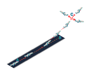
The ground operations on a vertiport terminal are similar to those of an airport, however, the difference lies in their arrival or departure operations. Figure 1(a) shows a conventional airport system where an aircraft occupies the runway, accelerates to the required ground speed, take-off, and after attaining a certain altitude will deviate in the direction of the approved flight plan. The two line segments “A to B” and “B to C” depict the common distance occupied by only one flight at a time, thus being a bottleneck to back-to-back departing traffic.
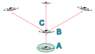
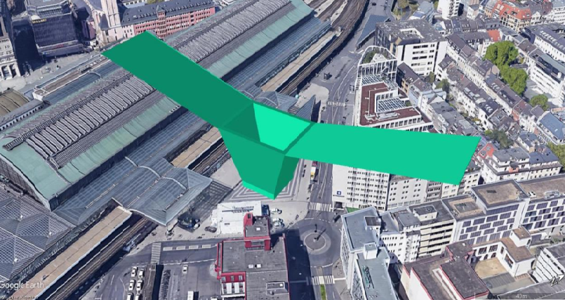
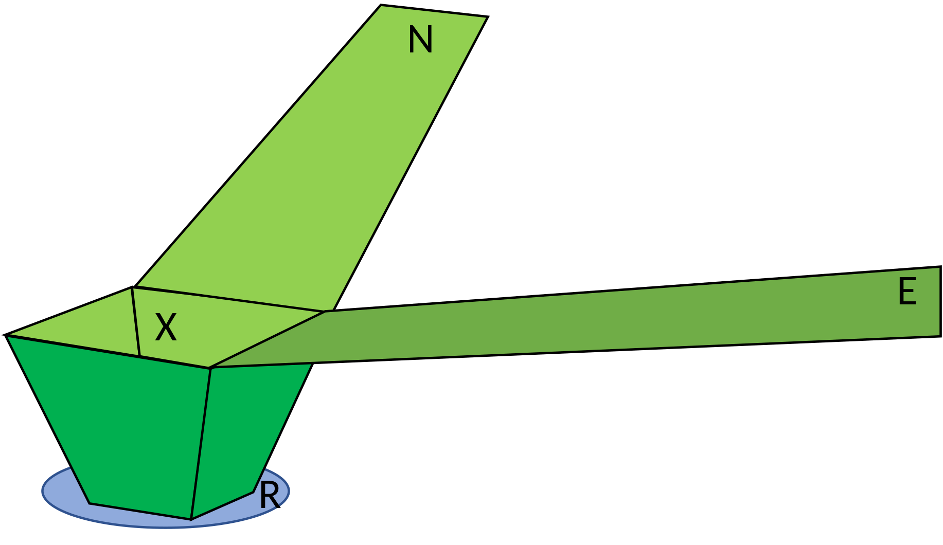
We define vertiminal as a vertiport terminal, which may be regarded as similar to a bus terminal, and a vertiport is like a bus stop. A vertiminal handles traffic of UAM VTOL capable aircraft. Such aircraft are defined as heavier-than-air aircraft, other than an aeroplane or helicopter, capable of performing VTOL using more than two lift or thrust units to provide lift during the take-off and landing [6]. A UAM aircraft departs from the Gate and travels a defined path on vertiminal called a taxiway, either on the ground or by air, before reaching the TLOF pad. Figure 1(b) shows a VTOL vehicle take-off from a TLOF pad. The line segment “A to B” shows the vertical take-off and unlike in Figure 1(a), the line segments “B to C” is of length. Unlike conventional runways, these pads are compact, and thus, a VTOL vehicle can reach cruising altitude (point C) quickly and start its approved flight plan. Figure 2 shows an example of Obstacle Free Volume (OFV), which is a funnel-shaped area with several climb surface directions (2 in Fig 2) available to the TLOF pad. The OFV guarantees that VTOLs can accomplish take-offs and landings within a sizable vertical segment, allowing them to account for environmental and noise limits in urban settings. At the end of the OFV boundary, there can be multiple climb surface directions for VTOL vehicles to climb to the vertiexit; an altitude where the UAM VTOL aircraft exits from the vertiminal airspace. A minimum separation time is required for successive take-offs and landing due to wake turbulence on the TLOF pad. Two UAM aircraft flying in the same surface direction must be separated by the minimum separation distance. However, this is not required to be maintained if the two aircraft fly in different surface directions. Hence, with more than one surface direction, the total delay can be reduced compared to a single surface direction, provided the scheduling algorithm takes advantage of the multiple directions when deciding the take-off/landing sequence. The addition of multiple directions thus effectively reduces shared path length and increases throughput.
A departure-ready flight can experience delays along its path due to the following:
-
1.
Separation requirements on the taxiways;
-
2.
TLOF pad availability while the previous VTOL aircraft climbs the OFV boundary;
-
3.
Wake turbulence time separation requirements on TLOF pad;
-
4.
Separation requirements on the climb surface direction in case multiple consecutive UAM vehicles take the same direction.
Arriving flights will experience similar delays — however, in the reverse order. Our goal is to formulate a scheduling problem to minimize a weighted sum of all such delays that should help improve the throughput of a vertiminal.
3.1 Problem Formulation
Given the number of UAM aircraft, their classes, their operation routes and their arrival & desired departure times, we need to design an efficient scheduling problem. We use a MILP technique to formulate the scheduling problem. The objective is to minimize the weighted sum of delays a UAM aircraft experiences during its complete operation. The time consumed on constrained resources like TLOF pads would be penalized more than the less constrained resources such as gates. The constraints for the objective problem are the physical constraint, separation requirements and other ATM regulations. We use the term VTOL or flight interchangeably instead of UAM aircraft throughout. We use the term “surface direction” in the optimization problem to denote both the take-off climb surface direction and approach surface direction. In Section 5.1, we will discuss the effect of multiple surface directions on departure delay experienced by different flight loads and their classes using the formulation presented in this section. We will also compare our formulation with First Come First Serve (FCFS) scheduling.
3.1.1 Assumptions
As explained below, several simplifying assumptions are made in modelling vertiminal operations.
-
•
Vertiminals will provide a standard fixed-width surface direction to ensure VTOL remains within this specified limit.
-
•
The approach or climbing speed of a VTOL is assumed to be given and governed by equipment type, environment and regulations.
-
•
Given a TLOF pad and a gate, the taxi route of each VTOL is predefined.
-
•
Nominal taxi speed is assumed to be given. Thus, given the length of the taxiway, the minimum and maximum travel time can be estimated.
-
•
The passage times at critical points along taxi routes, OFV and surface direction given by the solution to the optimization problem can be met by a VTOL. We also assume hovering is not allowed for VTOLs.
-
•
For the flights that do not have to turn around, gates act as a source of flights and vertiexit act as a sink of flights for the departures. While for arrivals, vertiexit is a source of flights, and gates act as a sink.
-
•
The number of VTOLs that have to turn around on the gates will not exceed the holding capacity of the gate.
-
•
At the gates, the flight whose boarding completes first will be ready to leave first.
| The set of gate nodes. Each physical gate node has an entrance node and an exit node . Each gate node has a holding capacity of . | |
| The set of nodes representing all TLOF pads at the vertiminal. Each TLOF pad has an entrance node and an exit node . | |
| The set of nodes representing OFV boundary on a TLOF pad | |
| The set of nodes representing the vertiexit reached from TLOF pad | |
| = ; = | |
| The set of all nodes on the ground, where a node could be the intersection of two taxiways, an entrance or exit to a taxiway or a TLOF pad. | |
| Set of links connecting gate nodes and taxiing nodes | |
| Set of links connecting taxing nodes nodes | |
| Set of links connecting taxing nodes and TLOF pads . | |
| Set of links connecting TLOF pads and OFV boundary | |
| Set of links connecting OFV boundary nodes and vertiexit nodes | |
| A link connecting nodes and also represented as (a,b). | |
| , The vertiminal network | |
3.1.2 VTOL Operations on a vertiminal
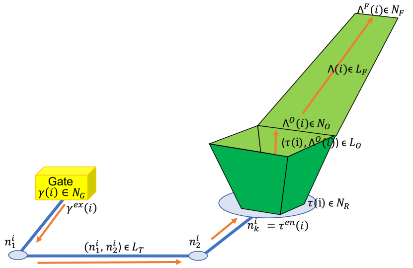
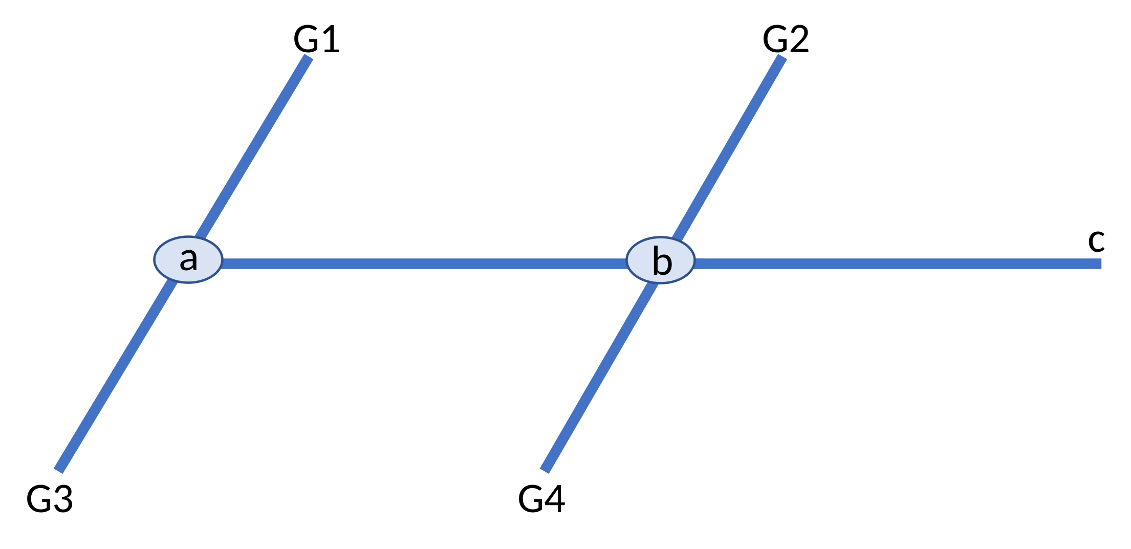
The Table 1 and Table 2 represent notation for a vertiminal and VTOL on a vertiminal, respectively. Figure 3 shows the nodes and links explained in Table 1. Let represent the physical taxi route for a VTOL , from its first node to its last node. is represented by an ordered set of nodes starting with the first node of the route, which is the exit of assigned TLOF pad for and gate exit for , progressing through the intermediate nodes and ending at the last node of route which is the gate entrance for or assigned TLOF pad entrance for , where denotes the total number of nodes involved in . represents taxiing route while represent taxiing route .
| The set of all VTOL. | |
|---|---|
| The set of all departing VTOL. | |
| The set of all arriving VTOL. | |
| , the set of VTOL that have to turn around. | |
| The set of all VTOL whose route passes through node . | |
| the time at which an arriving flight enters the airspace of vertiminal i.e. enters vertiexit. | |
| the time at which a departing flight is ready to leave the gate after passenger boarding. | |
| Gate assigned to VTOL | |
| Entrance node of gate assigned to VTOL | |
| Exit node of gate assigned to VTOL | |
| TLOF pad assigned to VTOL . is a TLOF pad assigned to while is assigned to . | |
| Entrance node of the TLOF pad assigned to VTOL . | |
| Exit node of the TLOF pad assigned to VTOL . | |
| Surface direction assigned to VTOL from TLOF pad . is the surface direction assigned to while is assigned to . | |
| Vertiexit node on surface direction . | |
| OFV boundary node on surface direction . | |
| Turn Around Time of VTOL . | |
| TLOF pad Occupancy Time of arriving VTOL . It is the time a VTOL takes to stop its motor and cool down before it can exit the TLOF pad. | |
| TLOF pad Occupancy Time of departing VTOL . It is the time a VTOL takes to reach the centre of the TLOF pad, start its motor, and prepare for take-off. | |
| Required safe separation time at landing or takeoff of VTOL from its immediate trailing VTOL , . |
A VTOL with a stop on the vertiminal will follow the following route:
-
1.
Link represents approach direction to the assigned TLOF pad .
-
2.
Link connecting OFV boundary node and TLOF pad .
-
3.
A sequentially ordered set of nodes , from the TLOF pad exit node to the entrance of the gate .
-
4.
For the turnaround flights , VTOL would be in the holding space of the gate , where boarding and deboarding occur.
-
5.
A sequentially ordered set of nodes , from the starting gate node to the entrance of the assigned TLOF pad
-
6.
Link connecting OFV boundary and TLOF pad .
-
7.
Link represents climb direction to the assigned TLOF pad .
| , Non-negative variable representing the time at which VTOL reaches node . Note that the VTOL does not slow down, let alone stop, before reaching a node and continues to achieve smooth travel unless the node is the exit or entrance of a TLOF pad or gate. | |
|---|---|
| Binary variable, indicating if VTOL reaches node before VTOL does. if and only if VTOL reaches node before VTOL does; otherwise. | |
| Binary variable used for selecting the minimum exit time for VTOLs in the Turn-Around Time (TAT) set. |
| Weight assigned to a departing VTOL for the time it expends at the gate. . | |
|---|---|
| Weight assigned to a departing VTOL for the taxiing time it expends. The requirement ensures that a VTOL should spend more time on the gate rather than on taxiways so as to avoid congestion and save energy. Also, it is beneficial for a multirotor to fly (in the case of air taxi) at the maximum optimal speed in order to reduce energy consumption[29]. | |
| Weight assigned to a VTOL for the time it spends on the TLOF pad and inside the OFV during take-off. TLOF pad and OFV are highly constrained resources and a bottleneck; hence, this weight value should be kept high. . | |
| Weight assigned to a VTOL for the time it spends inside the OFV and on the TLOF pad during landing. TLOF pad and OFV are highly constrained resources and a bottleneck; hence, this weight value should be kept high. . | |
| Weight assigned to an arriving VTOL for the taxiing time it expends. The requirement ensures that the VTOL will leave the TLOF pad at the earliest. | |
| Weight assigned to a departing VTOL to the time it expends to reach vertiexit from a TLOF pad. . | |
| Weight assigned to an arriving VTOL to the time it expends to reach the TLOF pad from a vertiexit. . | |
| Weight assigned to a VTOL for spending time on holding space of a gate. . |
3.1.3 Formulation
Objective function: minimizes the weighted sum of delays; equation(1)
-
•
For departures: (a) waiting at the departure gate, (b)while taxiing, (c) climbing inside OFV and (d) climbing time to vertiexit
-
•
For arrivals: (a) during approach, (b) leaving the TLOF pad and (c) reaching the gate
-
•
For turnaround VTOLs: turnaround time on the gates due to passenger boarding and deboarding.
The decision variables and weights are described in Table 3 and Table 4, respectively.
| (1) |
C1: We impose constraint equation (2) to ensure that an arriving VTOL starts on the approach surface direction starting from vertiexit.
| (2) |
C2: A VTOL traverses physical nodes while a VTOL traverses physical nodes . For speed control and smooth travel over all the links,i.e. taxiing ways, OFV and surface direction, constraint equation (3) is required. The terms are the respective minimum and maximum time taken by VTOL on the link .
| (3) |
C3: A VTOL will spend time on the gate not less than its turn around time, which is ensured by the constraint equation (4)
| (4) |
C4: The constraint equation (5) is the minimum time when the VTOL should leave the gate and start taxiing.
| (5) |
C5: Definition of Predecessors :
| (6a) |
| (6b) |
C6: The following constraint prevents overtaking in terms of :
| (7) |
C7: For preventing head-on collision of two VTOLs on a link , following constraint is used:
| (8) |
C8: This constraint maintains the separation requirement on the Taxi and surface direction, where is the separation requirement between VTOL in units of distance over the edge(or link) of length .
| (9) |
C9: The constraint (10) enforces the gate holding capacity of a gate that should not be exceeded. We have shown for holding capacity of 3. The equations (11d) linearize the constraint.
| (10) |
| (11a) | |||
| (11b) | |||
| (11c) | |||
| (11d) |
C10: Constraint equation (12) maintains the wake vortex requirement on the TLOF pad when a VTOL lands (or does a take-off) where is the minimum time VTOL should wait to either arrive or depart after the arrival(or departure) of VTOL .
| (12) |
C11: The time taken to reach the TLOF pad exit point upon landing is captured by constraint (13).
| (13) |
C12: The time taken to take-off after entering the TLOF pad from an entry point is captured by constraint (14). Constraint equations (14) and (13) along with (3) maintain the time continuity over the VTOL’s route.
| (14) |
C13: Upon arrival of VTOL , the following VTOL should reach the OFV boundary only after VTOL has left the TLOF pad through its exit point. Constraint equation (15) satisfies this requirement
| (15) |
C14: When a VTOL departs from the assigned TLOF pad, its immediate follower VTOL cannot enter the TLOF pad till VTOL has crossed its OFV boundary. Constraint equation (16) ensures this.
| (16) |
C15: A departing VTOL must enter a TLOF pad only after the arriving VTOL has left the TLOF pad.
| (17) |
C16: Binary and non-negativity constraints:
| (18a) | |||
| (18b) |
3.2 Comparison to the previous formulation
In our earlier work [28], we formulated the optimisation problem (opt A) with two binary variables: immediate predecessor and predecessor . Our present optimisation formulation (opt B) has eliminated the immediate predecessor variable because implicitly incorporates the information conveyed by . This change eliminated the need for a dummy VTOL and also resulted in a reduction of 10 constraints and thus, drastically reduces the time to reach the solution.
4 Throughput Capacity Equations
In the previous section, our objective was to minimize a weighted sum of delays, subject to constraints arising from vertiminal operations. While the weighted sum of delays is optimized, we do not know if the optimal strategy in Section 3.1 ends up affecting the throughput of the vertiminal. To answer this question, we study the maximum throughput that can be achieved – this is what we call “throughput capacity.” The capacity of the system comprising of: (a) gates at the apron, (b) taxiways and (c) TLOF pads would determine the maximum throughput capacity of a vertiminal. We analyze each of these elements independently and base our analysis on [31]. Finally, the throughput obtained using the optimal strategy in Section 3.1 is compared with the throughput capacity.
4.1 TLOF pad system
The TLOF pad system consists of TLOF pad, OFV and surface directions as illustrated in Figure 4. We analyse the throughput capacity by considering the arrivals and departures of VTOLs to and from the system. While a few factors such as visibility, precipitation, wind direction, etc. have been ignored, the following factors are considered in the capacity calculations:
-
•
Number of TLOF pads
-
•
Number of surface directions
-
•
Separation requirements between VTOLs imposed by the ATM system
-
•
Mix of VTOL classes using the vertiminal
-
•
Mix of movements such as arrivals, departures, or mixed on each TLOF pad and their sequencing
We define the term maximum throughput capacity as the maximum number of movements that can be performed in unit time on a TLOF pad without violating ATM rules such as wake vortex and other separation timing between two VTOLs. We first calculate for a single TLOF pad and then extend our calculations to multiple TLOF pads. On a TLOF pad, there are 4 possible sequences of movement pairs: Arrival-Arrival , Departure-Departure , Arrival-Departure and Departure-Arrival . Recall that ATM regulations require safe separation distance on surface directions and wake vortex time separation on the TLOF pad. These separation requirement values depend on the classes of the VTOLs involved. Additionally, during departure or arrival operations, only 1 VTOL can occupy the OFV. The throughput capacity is determined by the time separation enforced by ATM rules for various VTOL classes executing different movements.
The different time parameters we are going to utilise for analysis are:
-
1.
: The safe separation distance required on the surface direction between VTOL and , followed by , is converted into time separation (constraint equation (9)).
-
2.
: Wake vortex separation on TLOF pad between VTOL and
-
3.
: Occupancy time of a VTOL entering a TLOF pad before take-off or after landing on a TLOF pad before exit.
-
4.
: OFV travel time by a VTOL during departure or arrival, respectively.
-
5.
: Surface direction travel time by a VTOL during departure or arrival, respectively.
The following equations calculate the maximum time required in different sequences of movements , and VTOL is followed by VTOL .
-
•
Arrival-Arrival: Two VTOLs are arriving from vertiexit to the TLOF pad. If the VTOLs and are arriving from different surface directions, then set to 0.
(19) -
•
Departure-Departure: Two VTOLs are departing from the TLOF pad to vertiexit. If the VTOLs and are departing in different surface directions, then set to 0.
(20) -
•
Arrival-Departure: When an arrival is followed by a departure on a TLOF pad. In case the VTOLs and are using different surface directions, set to 0.
(21) -
•
Departure-Arrival: When a departure is followed by an arrival on a TLOF pad. In case the VTOLs and are using different surface directions, set to 0.
(22)
The maximum throughput of the movement pair per unit time is given as
| (23) |
The work in [31] calculates the expected capacity of a runway by considering all the possible aircraft classes and all possible permissible pairs of movements that have occurred in the past and then using a probability of occurrence for each of these events. Due to lack of any real-world data on UTM, our calculation is limited to the maximum throughput of any system. The maximum throughput of any movement pair is calculated by evaluating the VTOL classes that have minimum time parameter values. In the random sequence of arrivals and departures, the occurrence of movement pair has a low probability. Thus, we take the maximum time of the movement pairs to find the bottleneck in the system and define the capacity.
| (24) |
The maximum throughput capacity of the TLOF pad system, per unit time, is then given as:
| (25) |
A TLOF pad can facilitate both arrival and departure movements or can also cater to a single type of movement. In the case of a vertiminal equipped with multiple TLOF pads, its capacity is decided according to the configuration, i.e., there can be several combinations of assigning arrivals and departures movements to the TLOF pads. For instance, in a vertiminal with two TLOF pads, one configuration might utilize both pads for both arrival and departure. In contrast, another configuration might designate one TLOF pad exclusively for arrivals and the other for departures. In either case, the overall capacity of the vertiminal is determined by the combined throughput capacity of each individual TLOF pad.
| (26) |
where is calculated for each TLOF pad using equation (25) and is set of configuration.
4.2 Taxiway system
The traditional airport always has a taxiway running parallel to the runway. These long, well-designed taxiways are not a factor limiting the capacity of an airport. However, the taxiway system of vertiminal would be different as they are shorter, linking TLOF pads’ entry and exit points to the gate exit and entry points, respectively, as shown in Figure 5. There might be a single taxiway link or multiple taxiways with intersections among them on the vertiminal, each being a half-duplex link. Considering the gates and TLOF pads as sources and sinks, respectively (or even vice versa), the taxiway system can be conceptualized as a flow network problem. By deriving each link’s flow capacity, the flow network’s maximum capacity can be calculated using the max-flow min-cut theorem [32].
Each taxiway link has a static and dynamic capacity. Static capacity can be defined as the maximum number of stationary vehicles on it, while the dynamic capacity is the maximum number of vehicles passing through it per unit time, which is independent of taxiway length. Assuming uniform taxi velocities for all VTOL classes, the minimum sum of vehicle length and safe separation distance between two vehicles determines the dynamic capacity on any taxiway link and, thus, its flow rate. Given the size of the VTOL vehicle as , the separation distance and the maximum taxi-velocity of the VTOLs as , the maximum flow rate of a taxiway link can be calculated as:
| (27) |
If the three parameters in Equation (27) remain constant for each taxiway link, the maximum flow rate remains uniform across the entire taxiway network. However, varying and for each link necessitates the use of the max-flow min-cut theorem to calculate the overall maximum flow rate for the network().
4.3 Gate system
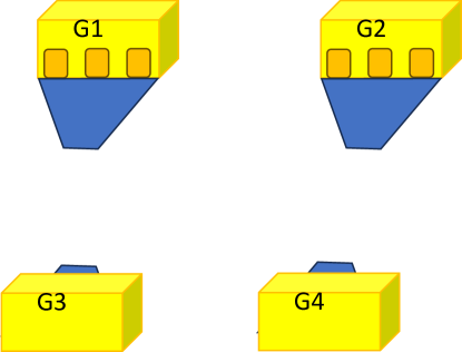
The gate system on a vertiminal can consist of multiple gates, each having multiple parking slots for VTOLs, as shown in Figure 6. The most basic and standard way to calculate the capacity of a gate system is the total number of VTOLs that can stand on a vertiminal simultaneously, referred to as static capacity (). However, a better measure of the capacity is the dynamic capacity, defined as the number of VTOLs per unit time that can be accommodated by the gate system and this is affected by the VTOLs’ turnaround times. For calculating the maximum throughput of the gate system, the class of vehicle having the minimum turnaround time should be considered. The maximum throughput is then calculated as:
| (28) |
Till now, we showed individual throughput calculations for TLOF pad, taxiway and gate systems considering them independently. The overall vertiminal’s throughput is limited by the minimum of the three systems as shown in equation (29).
| (29) |
5 Evaluation of the results
We used MATLAB version 2022a (9.12) with an optimization toolbox of version 9.3 on a Desktop PC equipped with an i7-11700F processor having 16 cores (8 physical) @ 2.5GHz and 64GB RAM to solve the optimization problem described in 3.1. Our implementation is available on GitHub for reproducibility [30].
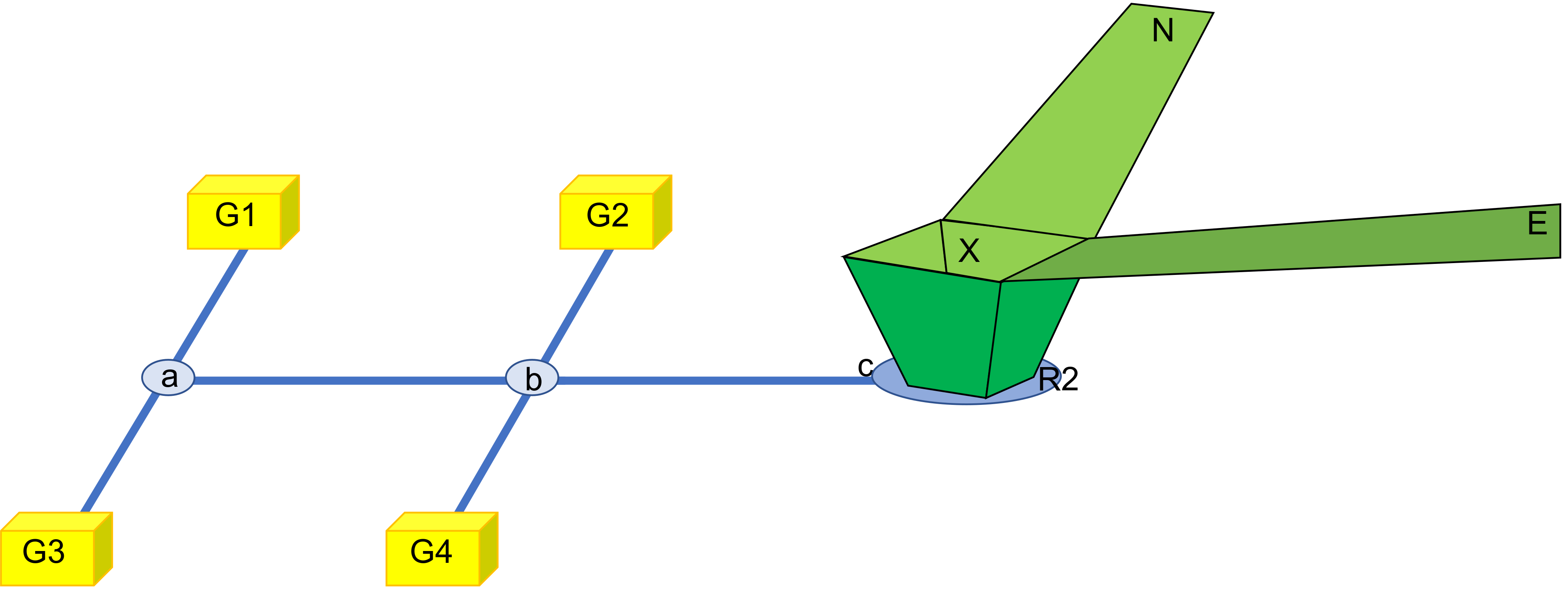
Figure 7 shows the topology used in our computational setup. All taxi edges in the network are equal in length, and similarly, all surface direction edges are equal. However, the length of the surface direction edges is greater than that of the taxi edges. The Table 5 mentions the weights used in objective (1) of MILP and other parameters that encompass several edge lengths and speeds. We randomly assign gate, surface direction, and to VTOLs. The large constant is set as .
| 0.2 | |
| 0.8 | |
| 1 | |
| 0.7 | |
| * | 0.1 |
| * | 0.7 |
| * | 1 |
| * | 0.8 |
| Gate taxiway length | 30 units |
| Taxiway edge length | 45 units |
| OFV length | 75 units |
| surface direction length | 300 |
| Average Taxi-speed | 6 units/sec |
| Maximum OFV climb speed | 17.14 units/sec |
| Maximum Surface direction speed | 23.73 units/sec |
| Separation distance on taxi (Small) | 5 units |
5.1 Results from the MILP formulation for VTOL departures
The solution provides the exact schedule of a VTOL movement from gate to vertiexit — the times at which a VTOL: (i) departs from the gate, (ii) crosses each node on in its path, (iv) arrives at the TLOF pad, (v) crosses OFV boundary and (vi) exits from the vertiexit.
The for a VTOL is calculated as , where is the desired time to depart from the gate and is time to reach the vertiexit. It is achievable only when no other VTOLs are present in the vertiminal. By comparing the actual time (provided by the MILP solution) with , we determine the ExcessDelay. Our goal is to observe the effect of multiple surface directions on ExcessDelay incurred by departing flights. We consider a total of surface directions from the OFV boundary (‘X’ in Figure 7). The total number of runs is 24 (6 different sets of flights and 4 directions). We compare the ExcessDelay obtained from our formulation with that of FCFS scheduling. Our implementation of FCFS uses the same set of constraints described in Section 3.1 with an additional constraint that forces the VTOLs to take off according to the order of their . We recall that a route is defined by the following elements: departing gate, a taxiing path from gate to TLOF pad, TLOF pad and surface direction. For comparison, in each run MILP and FCFS are provided with the same set of flights along with their route and .
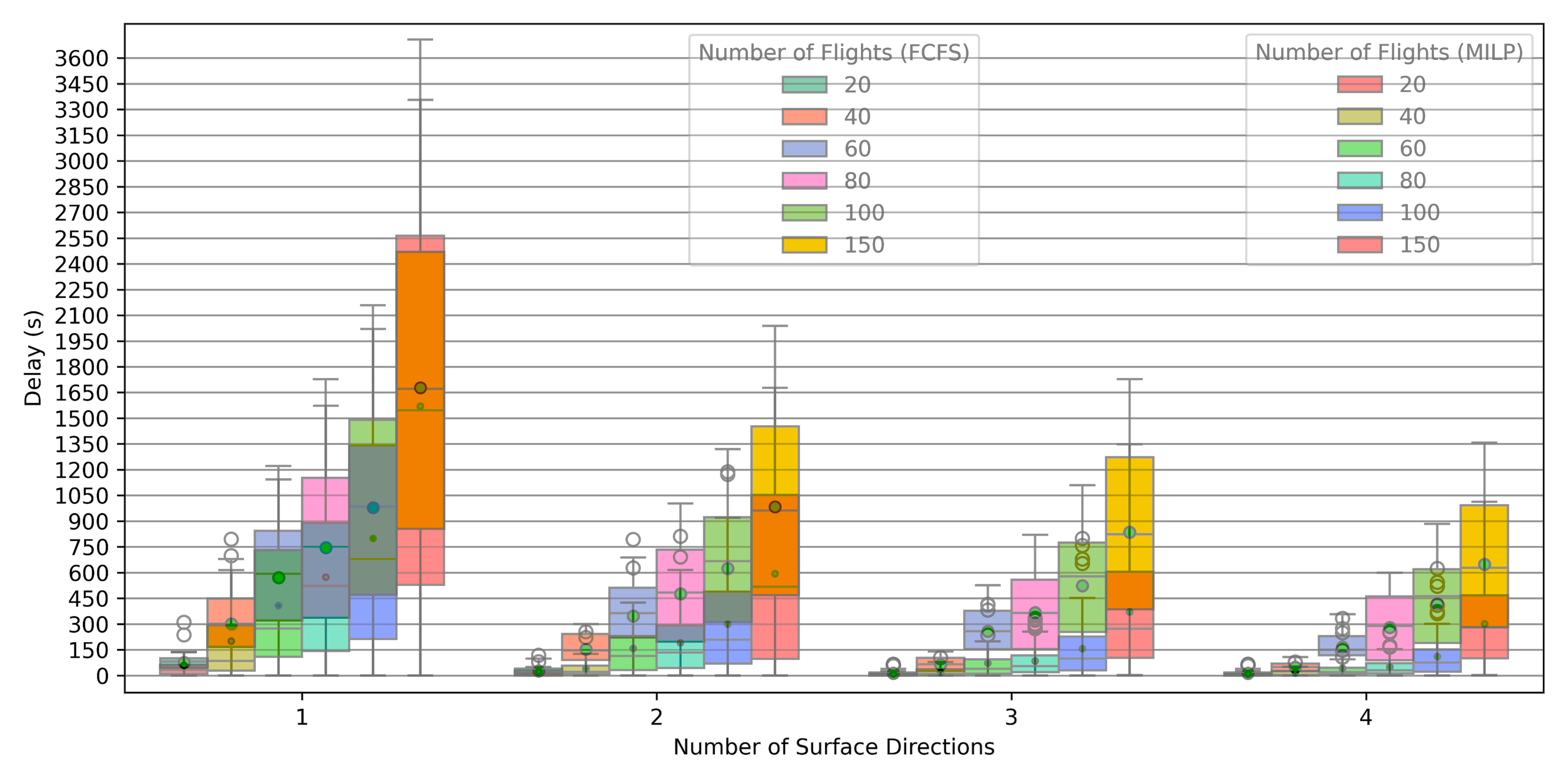
When two successive VTOLs use different surface directions, since there is no separtion requirement it is sufficient for the follower to take off by adhering only to wake vortex separation, thus reducing its overall delay i.e. ExcessDelay. This delay reduction is observed in Figure 8 by comparing delay distribution among flights with an increase in the number of surface directions. From Figure 8, we see a delay reduction of about 50% as we increase the number of surface directions from 1 to 2. Furthermore, as we increase the number of flights, the delay is increased due to congestion on vertiminal. An analysis of delay distribution for a flight set between our MILP and FCFS scheduling reveals notable differences. The third quartile (75%) of MILP is lower than the third quartile of FCFS (with exception of single surface direction and 150 flights). The mean and median of MILP are always less than that of FCFS. Our MILP delays tend to skew away from the maximum delay, as evidenced by a higher mean value than the median. In contrast, the FCFS delays are uniformly distributed among flights, with coinciding mean and median values. In the presence of multiple surface directions, our formulation provides a significantly lower mean delay. More than 50% of the flights have a 50% reduction in delay. In summary, our MILP formulation prioritizes on minimizing overall flight delays.
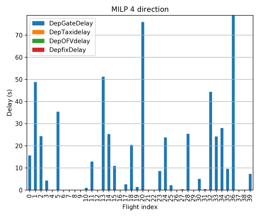
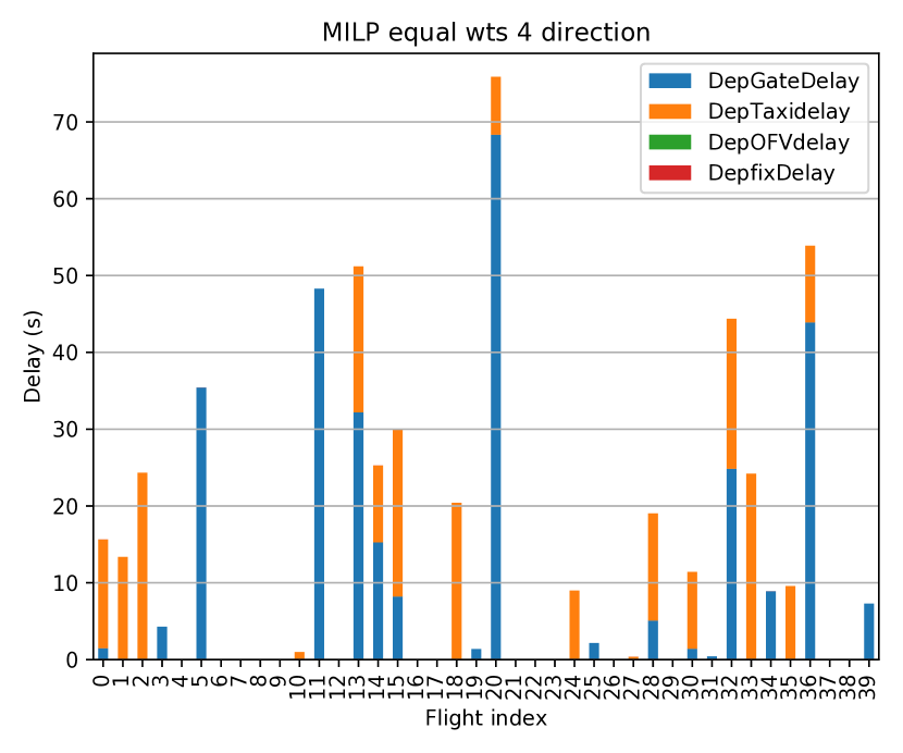
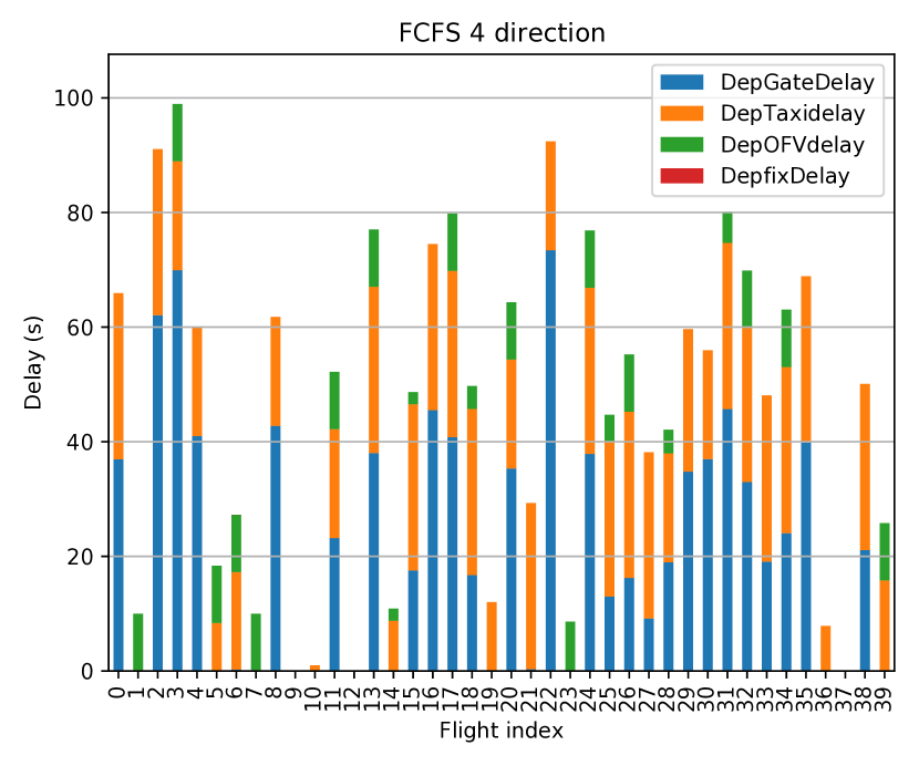
The bar plots shown in Figure 9 represents the distribution of ExcessDelay components such as gate delay (waiting at the gate), taxiing delay, OFV delay, and climb delay for each flight. Taxing delays signify congestion on taxiways, while OFV delay indicates a lack of availability of resources such as TLOF pad and OFV. Due to congestion on taxiways, a VTOL may not be able to fly or move at the optimal speed that may result in energy wastage [29]. Thus, taxi delays are undesirable and it is more energy-efficient to wait at the gate. We used 40 flights with 4 surface directions and compared the results with FCFS scheduling. Figure 9(a) shows the MILP formulation where all the flights experience only gate delay. Additionally, we analyze the impact of equal weights used in the objective to study the VTOL delay. This effectively changes the objective to minimize the sum of delay i.e., . Figure 9(b) shows the MILP with equal weights. The delay constitutes gate delay and taxiing delay. The taxiing delay (orange bars) occur as flights are slowly moving on taxiways instead of waiting at the gate even though the overall delay is at par with MILP (shown in Figure 9(a)). Figure 9(c) shows gate delay, taxiing delay and OFV delay (green bars) for FCFS scheduling. The OFV delay component is large compared to zero OFV delay in MILP. In summary, the delay breakup not only demonstrates the importance of weighted delays in the objective function, it also shows that FCFS scheduling leads to increased delay incurred by the VTOLs.
5.2 Results from Throughput Capacity
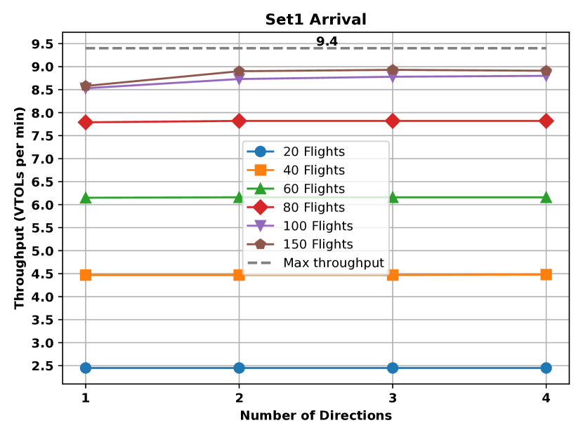
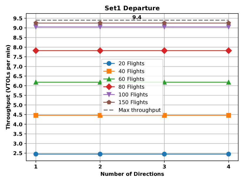
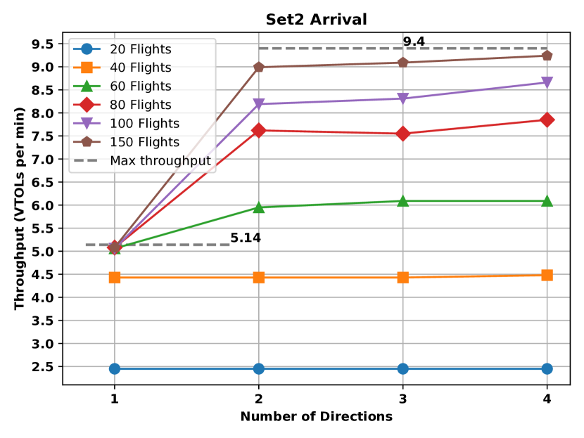
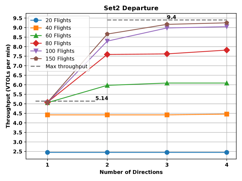
Recall that in Section 4, we discussed the capacity equations for: (a) TLOF pad system, (b) Taxiway system, and (c) Gate system. We determine the maximum achievable throughput of the vertiminal using the equations and the parameters shown in Table 5. We had considered the smallest class of VTOLs because they have the shortest turnaround time and minimum separation distance requirements. Using the time stamp of the VTOLs to reach the TLOF pad, we analyze the throughput achieved by the optimal strategy for solving the problem in Sec 3.1. We have varied the number of flights and the number of surface directions for all possible combinations of movements. For the TLOF pad system computation, we will use only (or ) where the vertiexit is a source (sink), and gates act as sinks (sources).
The following are the two sets of parameters used in comparison of throughput analysis using MILP and the equations from Section 4:
-
•
Set1: Separation requirement on surface direction is 75 units, Turn Around Time (TAT) on the gate is 90 seconds.
-
•
Set2: Separation requirement on surface direction is 280 units, Turn Around Time (TAT) on the gate is 120 seconds.
TLOF pad system:
| 4.41 s (Set1), 11.79 s (Set2) | |
| 0.833 s | |
| 2 s | |
| 4.375 s | |
| 12.65 s |
The time parameters described in the Section 4.1 equations (19)-(22), are presented in Table 6. We calculate the maximum time required for all the movement sequence pairs shown in Table 7. For Set1, the movement pair arrival-arrival or departure-departure gives the maximum achievable throughput () of VTOLs per minute. Whereas for Set2, the movement pair arrival-arrival or departure-departure gives the maximum achievable throughput () of VTOLs per minute for single surface direction and VTOLs per minute for multiple surface directions.
| Set | Surface Directions | Movement Pair | TLOF Times (s) |
|---|---|---|---|
| Single | 6.375 | ||
| 1 | Single | 19.02 | |
| Multiple | 6.375 | ||
| Multiple | 6.375 | ||
| Single | 11.67 | ||
| 2 | Single | 19.02 | |
| Multiple | 6.375 | ||
| Multiple | 6.375 |
If two consecutive VTOLs have different routes, then the separation requirement for the same surface direction, , is set to 0. In Set1, since the TLOF pad occupancy time and OFV travel time () is greater than , there is no advantage of multiple surface directions. In Set2, and thus having multiple surface directions gives a higher throughput. The same can be observed in Figures 10 - 11, which show the throughput achieved by solving the MILP formulation (1) with different number of flights and surface directions for the TLOF pad system. To observe the maximum throughput, the input number of flights needs to be significantly high. The plots of 100 and 150 flights thus validate both our MILP formulation and the throughput calculations, including the advantage of multiple surface directions as mentioned in Set2.
Gate system: Recall the topology shown in Figure 7 which has 4 gates with 3 parking slots each, resulting in a static capacity () of 12 VTOLs. For Set1, the gate system has a maximum dynamic capacity or throughput () of VTOLs per minute. For Set2, the throughput is VTOLs per minute.
Taxiway system: Using the equation (27) from Section 4.2, the maximum flow rate of the taxiway link is calculated to be VTOLs per minute, which represents the entire taxiway network. This is significantly higher than the maximum throughput of the TLOF pad system and Gate system, indicating that taxiway flow rate is not a limiting factor for vertiminal capacity.
Finally, We obtain the vertiminal’s maximum throughput using equation (29). For Set1 it is 8 VTOLs per minute, while for Set2, it is 5.14 VTOLs per minute for single surface direction and 6 VTOLs per minute for multiple surface directions.
Our throughput results also align with other works mentioned in [24]. The authors consider only consolidated arrival and departure times without any consideration of separation requirements. In contrast, from Section 4.1, for a single VTOL, arrival time = and departure time = , shows in detail the occupancy time of TLOF pad, OFV, and travel time on a surface direction. Furthermore, from equations (19) - (22), the TLOF pad throughput is affected by the maximum of individual time parameters rather than the consolidated arrival or departure time. By increasing any time parameter, arrival and/or departure time may increase, which decreases the throughput, thus validating the results shown in [24]. Consequently, the estimation of required for a single TLOF pad is shown in equation (30).
| (30) |
Unlike [24], our equations allow a detailed analyses of throughput of the TLOF pad system (), taxiway system () and the gate system (), and thus enables deeper understanding and the significance of the TLOF pad to gate ratio.
6 Conclusion
This paper is an extension to our previous work [28]. We have extended the optimization formulation to include arrival flights and flights with turnarounds at the gate, thus enabling optimization for a broader range of operations. We have shown that our formulation gives a 50% delay reduction as compared to FCFS scheduling. Our work delves deeper into vertiminal’s throughput by holistically analyzing its three core elements: the TLOF pad, taxiway network, and gates using the derived equations (19)-(28). We conducted computations to validate our optimization formulation and the accuracy of the throughput calculations. We further demonstrated that when the separation time requirement between flights is more than the occupancy time of OFV, multiple surface directions significantly affects the throughput. Thus, by providing precise throughput calculations using equations (without further simulations), our work empowers practitioners to optimize vertiminal design and operations for maximum efficiency.
For our further work, we will work on a case study using the design of Gimpo vertiminal [25] and find methods to decrease the computation time. One of the methods would be to use a rolling horizon which would also help in scalability. We can also make the optimization problem stochastic instead of deterministic operation. The formulation presented in this work does not consider Quality of Service (QoS), and hence, we will enhance this aspect. Future analysis would involve developing a capacity envelope for a vertiminal.
References
- [1] NASA. Uam vision concept of operations (conops) uam maturity level (uml) 4.
- [2] Future air mobility: Major developments in 2022 and significant milestones ahead, 2023.
- [3] Hayley Everett. Italy’s first vertiport deployed at fiumicino airport, 2022.
- [4] FutureFlight. Volocopter concludes european urban air mobility airspace integration flight trials, 2022.
- [5] FutureFlight. Advanced air mobility flight test site to open at german airport, 2023.
- [6] EASA. Prototype Technical Specifications for the Design of VFR Vertiports for Operation with Manned VTOL-Capable Aircraft Certified in the Enhanced Category.
- [7] FAA. ENGINEERING BRIEF #105 Vertiport Design.
- [8] UAE General Civil Aviation Authority, 2022.
- [9] J-B Gotteland and Nicolas Durand. Genetic algorithms applied to airport ground traffic optimization. In The 2003 Congress on Evolutionary Computation, 2003. CEC’03., volume 1, pages 544–551. IEEE, 2003.
- [10] Yu Jiang, Xinxing Xu, Honghai Zhang, and Yuxiao Luo. Taxiing route scheduling between taxiway and runway in hub airport. Mathematical Problems in Engineering, 2015, 2015.
- [11] Changyou Liu and Kaifeng Guo. Airport taxi scheduling optimization based on genetic algorithm. In 2010 International Conference on Computational Intelligence and Security, pages 205–208. IEEE, 2010.
- [12] Gillian Clare and Arthur G Richards. Optimization of taxiway routing and runway scheduling. IEEE Transactions on Intelligent Transportation Systems, 12(4):1000–1013, 2011.
- [13] Hanbong Lee and Hamsa Balakrishnan. A comparison of two optimization approaches for airport taxiway and runway scheduling. In 2012 IEEE/AIAA 31st Digital Avionics Systems Conference (DASC), pages 4E1–1. IEEE, 2012.
- [14] Ioannis Simaiakis. Analysis, modelling and control of the airport departure process. PhD thesis, Massachusetts Institute of Technology, 2013.
- [15] Peng Cheng, Xiang Zou, and Wenda Liu. Airport surface trajectory optimization considering runway exit selection. In 17th International IEEE Conference on Intelligent Transportation Systems (ITSC), pages 2656–2662. IEEE, 2014.
- [16] Floris Herrema, Ricky Curran, Sander Hartjes, Mohamed Ellejmi, Steven Bancroft, and Michael Schultz. A machine learning model to predict runway exit at vienna airport. Transportation Research Part E: Logistics and Transportation Review, 131:329–342, 2019.
- [17] Catherine Chalon Morgan, Mohamed Ellejmi, Floris Herrema, and Ricky Curran. Validation of the runway utilisation concept. 9th SESAR Innovation Days, 2019.
- [18] John A Behrends and John M Usher. Aircraft gate assignment: using a deterministic approach for integrating freight movement and aircraft taxiing. Computers & Industrial Engineering, 102:44–57, 2016.
- [19] Wu Deng, Junjie Xu, Huimin Zhao, and Yingjie Song. A novel gate resource allocation method using improved pso-based qea. IEEE Transactions on Intelligent Transportation Systems, 2020.
- [20] Wu Deng, Meng Sun, Huimin Zhao, Bo Li, and Chunxiao Wang. Study on an airport gate assignment method based on improved aco algorithm. Kybernetes, 47(1):20–43, 2017.
- [21] Imke C Kleinbekman, Mihaela A Mitici, and Peng Wei. evtol arrival sequencing and scheduling for on-demand urban air mobility. In 2018 IEEE/AIAA 37th Digital Avionics Systems Conference (DASC), pages 1–7. IEEE, 2018.
- [22] Quan Shao, Mengxue Shao, and Yang Lu. Terminal area control rules and evtol adaptive scheduling model for multi-vertiport system in urban air mobility. Transportation Research Part C: Emerging Technologies, 132:103385, 2021.
- [23] Hack Vázquez et al. Vertiport sizing and layout planning through integer programming in the context of urban air mobility, 2021.
- [24] Parker D Vascik and R John Hansman. Development of vertiport capacity envelopes and analysis of their sensitivity to topological and operational factors. In AIAA Scitech 2019 Forum, page 0526, 2019.
- [25] Byeongseon Ahn and Ho-Yon Hwang. Design criteria and accommodating capacity analysis of vertiports for urban air mobility and its application at gimpo airport in korea. Applied Sciences, 12(12):6077, 2022.
- [26] Lukas Preis and Mirko Hornung. A vertiport design heuristic to ensure efficient ground operations for urban air mobility. Applied Sciences, 12(14):7260, 2022.
- [27] H-S Jacob Tsao, Wenbin Wei, Agus Pratama, and JR Tsao. Integrated taxiing and take-off scheduling for optimization of airport surface operations. In Proc. 2nd Annual Conference of Indian Subcontinent Decision Science Institute (ISDSI 2009), pages 3–5, 2009.
- [28] Ravi Raj Saxena, Tejas Joshi, DK Yashashav, TV Prabhakar, and Joy Kuri. Integrated taxiing and tlof pad scheduling using different surface directions with fairness analysis. In 2023 IEEE 26th International Conference on Intelligent Transportation Systems (ITSC), pages 1747–1752. IEEE, 2023.
- [29] Ravi Raj Saxena, Joydeep Pal, Srinivasan Iyengar, Bhawana Chhaglani, Anurag Ghosh, Venkata N. Padmanabhan, and Prabhakar T. Venkata. Holistic energy awareness and robustness for intelligent drones. ACM Trans. Sen. Netw., jan 2024. Just Accepted.
- [30] https://github.com/rrsaxena92/Vertiport_schedule/.
- [31] Richard De Neufville. Airport systems planning, design, and management. In Air Transport Management, pages 79–96. Routledge, 2020.
- [32] Tom Leighton and Satish Rao. Multicommodity max-flow min-cut theorems and their use in designing approximation algorithms. J. ACM, 46(6):787–832, nov 1999.