Charged Rotating BTZ Black Hole In The Non-Extensive Generalizations of Gibbs Entropy

Abstract

We study the thermodynamics and thermodynamic geometry of the (2+1) dimensional charged rotating Banados-Teitelboim-Zanelli(CR-BTZ) black hole within the framework of non-extensive generalizations of Gibbs entropy. We write down the Bekenstein-Hawking(BH) entropy of the black hole in terms of the non-extensive entropies namely: Kaniadakis entropy, Renyi entropy, Sharma-Mittal entropy, Tsallis-Cirto and Barrow entropy. We investigate their impact on the thermodynamic phase structure and geometry of the CR-BTZ black hole in four different ensembles namely: the fixed $(J,Q)$ ensemble, fixed $(\Omega,\Phi)$ ensemble, fixed $(J,\Phi)$ ensemble and the fixed $(\Omega,Q)$ ensemble where $J,Q,\Omega$ and $\Phi$ represent the angular momentum, electric charge, angular velocity and electric potential of the CR-BTZ black hole respectively. We investigate the Ruppeiner and geometrothermodynamic(GTD) geometries of the black hole for all the non-extensive entropy cases. We find that there are Davies type phase transitions in the CR-BTZ black hole for the Kaniadakis entropy case for all the above mentioned thermodynamic ensembles. These Davies type phase transitions were not seen in the BH entropy case. We also find that the Ruppeiner and the GTD scalar for the Kaniadakis entropy show curvature singularities corresponding to these Davies type phase transitions in the CR-BTZ black hole.

I Introduction:

It is by now well known that black holes are thermodynamic objects characterized with a temperature (Hawking temperature) proportional to surface gravity at its horizon and entropy (Bekenstein-Hawking entropy) proportional to the horizon area [1, 2].

$$T=\frac{\kappa}{2\pi},~{}~{}~{}~{}~{}~{}~{}~{}S_{BH}=\frac{A}{4}$$ (1)

These two quantities ($T$ and $S_{BH}$) constitute the basis of what is now known as black hole thermodynamics [3]. Over the years, black hole thermodynamics has evolved into an active area of research with a number of generalizations of its originial version [4, 5, 6, 7, 8, 9] shedding light on the phase structures of black holes.

An important issue in the context of black hole thermodynamics that has recently come to focus is the modification of black hole entropy owing to different corrections. These corrections result in a number of non-extensive generalizations of Gibbs entropy. Some of these notable entropies are: Kaniadakis entropy, [10, 11], Renyi entropy [12], Sharma-Mittal entropy [13], Tsallis-Cirto [14] and Barrow entropy [15]. A brief introduction to these entropies will be provided in the next section. The impact of these entropies on the thermodynamic behaviour of a few black holes have been studied in a number of works [16, 17, 18, 19, 20]. Previously these entropy systems have been tested in cosmology [21, 22, 23] and quantum physics [24, 25, 26] with notable success.

Although black hole thermodynamics in its different forms have largely been successful in providing deep insights about the thermodynamic properties of black holes, there are a number of important issues which are far from being completely understood. One such issue is the microscopic origin of Bekenstein-Hawking(BH) entropy. In absence of a complete theory of quantum gravity, thermodynamic geometry studies of black holes have been used to extract qualitative ideas about microscopic interaction in black holes [27, 28, 29, 30]. Thermodynamic geometry is a key concept in the study of black holes as they provide an understanding of the phase transitions in terms of the curvature singularities obtained through a particular thermodynamic metric. Three such metrics which have been used in black hole thermodynamics are Weinhold, Ruppeiner and geometrothermodynamic metric (GTD).

Weinhold [31] introduced a Riemannian metric in the equilibrium space which is defined as the second derivative of the internal energy with respect to other extensive variables. The Weinhold metric is defined as:

$$g_{ij}^{W}=\partial_{i}\partial_{j}U(S,X)$$

where the internal energy ‘$U(S,X)$’ is a function of entropy S and other extensive variables X, where $X=(J,Q)$ for the case of charged rotating black hole.

Ruppeiner [32] later introduced a Riemannian metric which is defined as the negative hessian of the entropy with respect to the other extensive variables. The Ruppeiner metric is a concept based on the thermodynamic fluctuation theory of equilibrium thermodynamics, where the thermodynamic length is related to the probability of fluctuation between two states of the thermodynamic system [33]. The two are inversely related as an increase in the probability of fluctuation would mean a significant decrease in the thermodynamic length and vice-versa. The Ruppeiner metric is defined as:

$$g_{ij}^{R}=-\partial_{i}\partial_{j}S(U,X)$$

where the entropy ‘$S(U,X)$’ is a function of internal energy $U$ and other extensive variables X, where $X=(J,Q)$ for a charged, rotating black hole. The Riemannian scalar which is defined here as ‘$R_{rupp}$’ is a scalar invariant function in thermodynamic geometry. The sign of the scalar curvature has been linked to the nature of microscopic interactions in the thermodynamic system. For positive or negative scalar curvatures, the underlying interaction is either repulsive or attractive accordingly. Whereas the null curvature would mean an absence of interaction with a flat thermodynamic geometry. The Ruppeiner and the Weinhold metrics are conformally related to each other by the following relation [34, 35]:

$$g_{ij}^{R}dU^{i}dU^{j}=\frac{1}{T}g_{ij}^{W}dS^{i}dS^{j}$$ (2)

where $T=\frac{\partial{U}}{\partial{S}}$ is the Hawking temperature of the system with $U^{i}=(U,X)$ and $S^{i}=(S,X)$.

The Ruppeiner and Weinhold geometries have successfully predicted the occurrence of phase transitions in the case of ordinary thermodynamic systems. However there has been contradictory results for the case of black holes where for instance in Kerr-black hole [36] the Weinhold metric showed no phase transition whereas the Ruppeiner metric could show phase transitions only for a specific thermodynamic potential. However such problems were successfully addressed in the new geometric formalism of geometrothermodynamics(GTD)[37] where the properties of the phase space and the space of equilibrium states could be unified [38]. The GTD metric is a Legendre invariant metric and therefore would not depend on any specific choice of thermodynamic potential. The phase transitions obtained from the specific heat capacity of the black hole are properly contained in the scalar curvature of the GTD metric, such that a curvature singularity in the GTD scalar ‘$R_{GTD}$’ would imply the occurrence of a phase transition. The general form of the GTD metric is given by [39]:

$$g=\left(E^{c}\frac{\partial{\varphi}}{\partial{E^{c}}}\right)\left(\eta_{ab}\delta^{bc}\frac{\partial^{2}\varphi}{\partial E^{c}\partial E^{d}}dE^{a}dE^{d}\right)$$ (3)

where ‘$\varphi$’ is the thermodynamic potential and ‘$E^{a}$’ is an extensive thermodynamic variable with $a=1,2,3....$.

In this paper, we study the thermodynamics and thermodynamic geometry of the (2+1) dimensional charged rotating Banados-Teitelboim-Zanelli(CR-BTZ) black hole [27, 40] within the framework of non-extensive generalizations of Gibbs entropy. We write down the Bekenstein-Hawking(BH) entropy of the black hole in terms of the non-extensive entropies namely: Kaniadakis entropy, Renyi entropy, Sharma-Mittal entropy, Tsallis-Cirto and Barrow entropy. We investigate their impact on the thermodynamic phase structure and geometry of the CR-BTZ black hole in four different ensembles namely: the fixed $(J,Q)$ ensemble, fixed $(\Omega,\Phi)$ ensemble, fixed $(J,\Phi)$ ensemble and the fixed $(\Omega,Q)$ ensemble where $J,Q,\Omega$ and $\Phi$ represent the angular momentum, electric charge, angular velocity and electric potential of the CR-BTZ black hole respectively. We investigate the Ruppeiner and geometrothermodynamic(GTD) geometries of the black hole for all the non-extensive entropy cases.

The paper is structured as follows: in section II we review some known facts about the non-extensive generalisations of Gibbs entropy. The section III is about the CR-BTZ black hole system and its thermodynamic investigation within the framework of non-extensive entropies in various ensembles. In section IV we examine the thermodynamic geometry of the black hole system both in Ruppeiner and in the GTD formalisms. The final section contains our conclusions.

II Non-extensive generalizations of gibbs entropy

The entropy of a black hole scales with its area rather than its volume and is therefore regarded as a non-extensive quantity. Due to its non-extensive nature the black hole entropy is also non-additive and follows a non-additive composition rule [alonso2021nonextensive]. But in the case of Gibbs thermodynamics the entropy is defined to be both extensive and additive as it scales with the size of the system. However, the assumption of extensivity of Gibbs entropy is due to ignoring the long range forces that are prevalent between the thermodynamic sub-systems. Gibbs thermodynamics ignores these forces because the size of the system exceeds the interaction range between the thermodynamic sub-systems. The total entropy thus becomes equal to the sum of the entropies of its components. It therefore grows with the size of the thermodynamic system.

But these long range forces are important in various thermodynamic systems such as black holes. We can therefore infer that Gibbs thermodynamics may not be a suitable choice for studying black hole thermodynamics. Therefore in order to understand the non-extensive nature of black hole entropy, several non-extensive generalizations of Gibbs entropy have been prescribed. We give a brief outline of a few of those entropies below which we will use later in oder to study the thermodynamics and thermodynamic geometry of charged rotating BTZ black hole:

A. Kaniadakis entropy

Kaniadakis entropy[10, 11, 16, 41, 42, 43, 44] is a result of the lorentz transformations in special relativity. It is a relativistic non-extensive generalisation of gibbs entropy . The Kaniadakis entropy is defined as:

$$S_{K}=Log_{K}\Omega$$

$$S_{K}=\frac{\Omega^{K}-\Omega^{-K}}{2K}$$

where ‘$\Omega$’ is the number of microstates of the thermodynamic system and ‘K’ is the kaniadakis parameter which is connected to the rest energy of various parts of the relativistic system.
Considering $S_{BH}=Log\Omega$, the above equation can be modified into:

$$S_{K}=\frac{Sinh[KS_{BH}]}{K}$$ (4)

where, for the limit $K\rightarrow 0$, $S_{K}\rightarrow S_{BH}$

B. Renyi entropy

The Renyi entropy[45, 46, 47, 48, 49, 50, 51] is a measure of the quantum entanglement of a system. A phenomena where the quantum states of two or more particles could become correlated. It is defined as:

$$S_{R}=\frac{\ln\left[\sum_{i}P^{q}(i)\right]}{1-q}$$

where ‘P(i)’ is the probability distribution and ‘q’ is the non-extensive parameter.
By assuming that the Bekenstein Hawking entropy is just the Tsallis entropy, the Renyi entropy could be defined as:

$$S_{R}=\frac{\ln[1+\lambda S_{BH}]}{\lambda}$$ (5)

where ‘$\lambda$’ is the Renyi parameter and for the limit $\lambda\rightarrow 0$, $S_{R}\rightarrow S_{BH}$

C. Sharma-Mittal entropy

It is an entropy that generalises both the Renyi and the Tsallis entropies[13, 18, 52, 53, 54]. It is defined as:

$$S_{SM}=\frac{\left[\left(\sum_{i=1}^{w}P_{i}^{\left(1-\lambda\right)}\right)^{\frac{\rho}{\lambda}}-1\right]}{\rho}$$

where ‘$\rho$’ here is the new free parameter that is introduced in this case. By the same logic as before the Sharma-Mittal entropy could be written as:

$$S_{SM}=\frac{\left[\left(1+\lambda S_{BH}\right)^{\frac{\rho}{\lambda}}-1\right]}{\rho}$$ (6)

where, for the limit $\rho\rightarrow\lambda$, $S_{SM}\rightarrow S_{BH}$

D. Tsallis-Cirto entropy

In order to generalize the Gibbs entropy so as to maintain the extensivity of non-standard thermodynamic systems such as black holes. Tsallis and Cirto defined a new entropy which is given by[14, 55] :

$$S_{\delta}=(S_{BH})^{\delta}$$ (7)

where, $\delta\geq 0$ is a real parameter. For the limit $\delta\rightarrow 1$, $S_{\delta}\rightarrow S_{BH}$ and for $\delta=2$, $S_{\delta}$ becomes proportional to the volume of the $(2+1)$ dimensional CR-BTZ black hole.

E. Barrow entropy

The Barrow entropy[15, 56, 57] is proposed to measure the entropy of a black hole system whose smooth horizon has been replaced by the rough fractal structures. The Barrow entropy is formulated as:

$$S_{\Delta}=(S_{BH})^{1+\Delta/2}$$ (8)

where, ‘$\Delta$’ is the parameter that is linked to the fractal structure of the system with range $0<\Delta\leq 2$. where $\Delta\rightarrow 2$ would yield maximal fractal structure.And for the limit $\Delta\rightarrow 0$, $S_{\Delta}\rightarrow S_{BH}$

III Thermodynamics of the charged rotating BTZ black hole

The action which facilitates the field equations[58, 59, 60, 61, 62] from which the charged $(2+1)$ dimensional BTZ black hole solutions are obtained is given as:

$$I=\frac{1}{2\pi}\int d^{3}x\sqrt{-g}\biggl{(}R+2\Lambda-\frac{\pi}{2}F_{\mu\nu}F^{\mu\nu}\biggr{)}$$

where the Einstein’s field equations and the energy momentum tensor of the electromagnetic field are given by:

$$G_{\mu\nu}-\Lambda g_{\mu\nu}=\pi T_{\mu\nu}$$

and the energy momentum tensor for the same is given as:

$$T_{\mu\nu}=F_{\mu\rho}F_{\nu\sigma}g^{\rho\sigma}-\frac{1}{4}g_{\mu\nu}F^{2}$$

The line element that corresponds to the given solution is:

$$ds^{2}=-f(r)dt^{2}+\frac{dr^{2}}{f(r)}+r^{2}\biggl{(}d\phi^{2}-\frac{J}{2r^{2}}dt\biggr{)}^{2}$$

where $f(r)=-M+\frac{r^{2}}{l^{2}}+\frac{J^{2}}{4r^{2}}-\frac{\pi Q^{2}}{2}\ln\left[r\right]$ and ‘M’, ‘J’ and ‘Q’ are the mass, angular momentum and charge carried by the black hole. Solving the function for $f(r)=0$ would give us the roots which determine the horizon radius. For an exterior horizon radius ‘$r_{+}$’ the black hole mass is given by:

$$M=\frac{r_{+}^{2}}{l^{2}}+\frac{J^{2}}{4r_{+}^{2}}-\frac{\pi}{2}Q^{2}\ln\left[r_{+}\right]$$ (9)

and the black hole entropy is given by:

$$S_{BH}=4\pi r_{+}$$

III.1 The Kaniadakis entropy case

The Kaniadakis entropy, $S_{K}$ in terms of the black hole entropy, $S_{BH}$ is given by (4) as:

$$S_{K}=\frac{Sinh(KS_{BH})}{K}$$

where ‘K’ is the Kaniadakis parameter and for $K\rightarrow 0$, $S_{K}\rightarrow S_{BH}$. Starting with the above equation we get the modified horizon radius for the CR-BTZ black hole as:

$$S_{K}=\frac{Sinh(4\pi Kr_{+})}{K}$$

$$r_{+}=\frac{ArcSinh(KS_{K})}{4\pi K}$$ (10)

Fixed $(J,Q)$ ensemble:

We replace the horizon radius in (9) by the one obtained in (10) to get the modified mass $M_{K}$ for the CR-BTZ black hole which is given by :

$$M_{K}=\frac{4\pi^{2}K^{2}J^{2}}{ArcSinh^{2}[KS_{K}]}+\frac{ArcSinh^{2}[KS_{K}]}{16\pi^{2}l^{2}K^{2}}-\frac{\pi Q^{2}}{2}\ln\biggl{[}\frac{ArcSinh[KS_{K}]}{4\pi K}\biggr{]}$$

The function, $ArcSinh[KS_{K}]$ can be replaced by its logarithmic form, $\ln\biggl{[}KS_{K}+\sqrt{1+K^{2}S_{K}^{2}}\biggr{]}$ and therefore the expression for mass becomes:

$$M_{K}=\frac{4\pi^{2}K^{2}J^{2}}{Log[KS_{K}+\sqrt{1+K^{2}S_{K}^{2}}]^{2}}+\frac{\ln[KS_{K}+\sqrt{1+K^{2}S_{K}^{2}}]^{2}}{16\pi^{2}l^{2}K^{2}}-\frac{\pi Q^{2}}{2}\ln\biggl{[}\frac{\ln[KS_{K}+\sqrt{1+K^{2}S_{K}^{2}}]}{4\pi K}\biggr{]}$$ (11)

The heat capacity for the Kaniadakis entropy case in the fixed $(J,Q)$ ensemble can be obtained as:

$$C_{K}=\frac{\frac{\partial M_{K}}{\partial S_{K}}}{\frac{\partial^{2}M_{K}}{\partial S_{K}^{2}}}=-\frac{A}{B}$$ (12)

where,

$$A=\biggl{(}\ln[KS_{K}+\sqrt{1+K^{2}S_{K}^{2}}]\bigg{(}64J^{2}K^{4}\pi^{4}+4K^{2}\pi^{3}Q^{2}\ln[KS_{K}+\sqrt{1+K^{2}S_{K}^{2}}]^{2}\\ -\ln[KS_{K}+\sqrt{1+K^{2}S_{K}^{2}}]^{4}(1+K^{2}S_{K}^{2})\bigg{)}\biggr{)}$$ (13)

and

$$B=K\biggl{(}64S_{K}J^{2}K^{5}\pi^{4}\ln[KS_{K}+\sqrt{1+K^{2}S_{K}^{2}}]+4S_{K}K^{3}\pi^{3}Q^{2}\ln[KS_{K}+\sqrt{1+K^{2}S_{K}^{2}}]^{3}\\ -KS_{K}\ln[KS_{K}+\sqrt{1+K^{2}S_{K}^{2}}]^{5}+192J^{2}k^{4}\pi^{4}\sqrt{1+K^{2}S_{K}^{2}}+4K^{2}\pi^{3}Q^{2}\ln[KS_{K}+\sqrt{1+K^{2}S_{K}^{2}}]^{2}\sqrt{1+K^{2}S_{K}^{2}}\\ +\ln[KS_{K}+\sqrt{1+K^{2}S_{K}^{2}}]^{4}\sqrt{1+K^{2}S_{K}^{2}}\biggr{)}$$ (14)

In Fig.1 the heat capacity, $C_{K}$ is plotted against the Kaniadakis entropy, $S_{K}$ for $l=1,J=1$ and $Q=2$ in the fixed $(J,Q)$ ensemble. Here the solid blue curve represents the heat capacity for the Kaniadakis parameter, $K=0.012$ whereas the black dashed line represents the heat capacity for the Bekenstein-Hawking(BH) entropy case $(K=0)$. We find that for $K=0.012$, the heat capacity has a divergence at $S_{K}=137.69$ which indicates the presence of a Davies type phase transition present in the Kaniadakis modified black hole whereas the heat capacity for the BH entropy case shows no such behaviour.

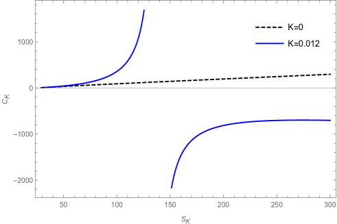
Figure 1: The heat capacity versus Kaniadakis entropy plot in the fixed $(J,Q)$ ensemble for $l=1,J=1$ and $Q=2$

Fixed $(\Omega,\Phi)$ ensemble:

The modified mass for the Kaniadakis entropy case in the fixed $(\Omega,\Phi)$ ensemble is given by:

$$M_{K}^{\prime}=M_{K}-J\frac{\partial M_{K}}{\partial J}-Q\frac{\partial M_{K}}{\partial Q}$$

$$M_{K}^{\prime}=M_{K}-J\Omega-Q\Phi$$

where $M_{K}^{\prime}$ is the modified mass for this ensemble and $\Omega$ and $\Phi$ are the angular velocity and electric potential of the black hole respectively. By making the necessary replacements and putting $l=1$, we get the final equation as follows:

$$M_{K}=\frac{(1-\Omega^{2})\ln[KS_{K}+\sqrt{1+K^{2}S_{K}^{2}}]^{2}}{16\pi^{2}}-\frac{\Phi^{2}}{2\pi}\left(\frac{2\ln\biggl{[}\frac{K}{\ln[KS_{K}+\sqrt{1+K^{2}S_{K}^{2}}]^{2}}\biggr{]}+\biggl{[}\frac{4\pi\ln[KS_{K}+\sqrt{1+K^{2}S_{K}^{2}}]^{2}}{K}\biggr{]}}{\ln\biggl{[}\frac{4k\pi}{\ln[KS_{K}+\sqrt{1+K^{2}S_{K}^{2}}]^{2}}\biggr{]}^{2}}\right)$$ (15)

We have here used the term $M_{K}$ instead of $M_{K}^{\prime}$ for convenience. Here $M_{K}$ is the modified mass for the fixed $(\Omega,\Phi)$ ensemble.

The heat capacity for the Kaniadakis entropy case in the fixed $(\Omega,\Phi)$ ensemble can be obtained as:

$$C_{K}=\frac{\frac{\partial M_{K}}{\partial S_{K}}}{\frac{\partial^{2}M_{K}}{\partial S_{K}^{2}}}\\ =-\frac{A}{B}$$

where,

$$A=\left(1+K^{2}S_{K}^{2}\right)\ln\left[KS_{K}+\sqrt{1+K^{2}S_{K}^{2}}\right]\ln\left[\frac{4K\pi}{\ln[KS_{K}+\sqrt{1+K^{2}S_{K}^{2}}]}\right]\\ \biggl{(}12K^{2}\pi\Phi^{2}\ln\left[\frac{4K\pi}{\ln[KS_{K}+\sqrt{1+K^{2}S_{K}^{2}}]}\right]+(-1+\Omega^{2})\ln[KS_{K}+\sqrt{1+K^{2}S_{K}^{2}}]^{2}\ln\left[\frac{4K\pi}{\ln[KS_{K}+\sqrt{1+K^{2}S_{K}^{2}}]}\right]^{3}\\ +8K^{2}\pi\Phi^{2}\ln\left[\frac{\ln[KS_{K}+\sqrt{1+K^{2}S_{K}^{2}}]}{4K\pi}\right]\biggr{)}$$ (16)

and

$$B=12K^{3}\pi\Phi^{2}(\sqrt{1+K^{2}S_{K}^{2}}+KS_{K}\ln(KS_{K}+\sqrt{1+K^{2}S_{K}^{2}}))\ln\bigg{(}\frac{4K\pi}{\ln(KS_{K}+\sqrt{1+K^{2}S_{K}^{2}})}\bigg{)}^{2}+\\ K(-1+\Omega^{2})\ln(KS_{K}+\sqrt{1+K^{2}S_{K}^{2}})^{2}(-\sqrt{1+K^{2}S_{K}^{2}}+KS_{K}\ln(KS_{K}+\sqrt{1+K^{2}S_{K}^{2}}))\ln\bigg{(}\frac{4K\pi}{\ln(KS_{K}+\sqrt{1+K^{2}S_{K}^{2}})}\bigg{)}^{4}\\ -8K^{3}\pi\Phi^{2}\ln\bigg{(}\frac{4K\pi}{\ln(KS_{K}+\sqrt{1+K^{2}S_{K}^{2}})}\bigg{)}\bigg{(}KS_{K}\ln(KS_{K}+\\ \sqrt{1+K^{2}S_{K}^{2}})(\ln\bigg{(}\frac{4K\pi}{\ln(KS_{K}+\sqrt{1+K^{2}S_{K}^{2}})}\bigg{)})\bigg{)}+\sqrt{1+K^{2}S_{K}^{2}}(4+\ln\bigg{(}\frac{4K\pi}{\ln(KS_{K}+\sqrt{1+K^{2}S_{K}^{2}})}\bigg{)})\\ -24K^{3}\pi\sqrt{1+K^{2}S_{K}^{2}}\Phi^{2}\ln\bigg{(}\frac{\ln(KS_{K}+\sqrt{1+K^{2}S_{K}^{2}})}{4K\pi}\bigg{)}$$ (17)

We see from Fig.2 that the heat capacity, $C_{K}$ for the charged rotating BTZ black hole is plotted against the Kaniadakis entropy, $S_{K}$ in the fixed $(\Omega,\Phi)$ ensemble. We draw the same plot in two different entropy ranges so as to make all the appearing divergences in the heat capacity curve visible. We see from Fig.2(a) that for $l=1,\Omega=0.2$ and $\Phi=0.1$ there is a divergence at $S_{K}=11.10$ for $K=0.012$ as shown by the solid blue curve. The heat capacity in the Bekenstein-Hawking(BH) entropy case ($K=0)$ here also produces a divergence at $S_{K}=11.08$ as shown by the black dashed curve. In Fig.2(b) we see that there is a divergence in the heat capacity curve at $S_{K}=125.74$ for $K=0.012$ whereas here the heat capacity in the BH entropy case $(K=0)$ remains a monotonically increasing function of entropy with no divergences.

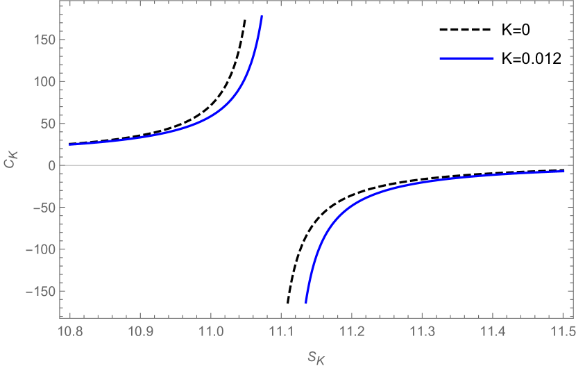
(a) For the range $10.8<S_{K}<11.5$

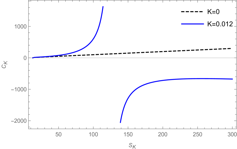
(b) For the range $10<S_{K}<300$

Figure 2: The heat capacity versus Kaniadakis entropy plots in the fixed $(\Omega,\Phi)$ ensemble for $l=1,\Omega=0.2$ and $\Phi=0.1$.

Fixed $(J,\Phi)$ ensemble:

The modified mass for the Kaniadakis entropy case in the fixed $(J,\Phi)$ ensemble is given by :

$$M_{K}^{\prime}=M_{K}-Q\frac{\partial M_{K}}{\partial Q}$$

where $\frac{\partial M_{K}}{\partial Q}=\Phi$ is the electric potential of the black hole with respect to the electric charge Q. By writing the term $M_{K}^{\prime}$ as $M_{K}$ for convenience we get:

$$M_{K}=\frac{\Phi^{2}}{2\pi\ln[\frac{4\pi}{S_{K}}]^{2}}\left(\ln\left[\frac{4\pi K}{\ln[KS_{K}+\sqrt{1+K^{2}S_{K}^{2}}]}\right]-2\ln\left[\frac{4\pi}{S_{K}}\right]\right)+\frac{4\pi^{2}K^{2}J^{2}}{\ln[KS_{K}+\sqrt{1+K^{2}S_{K}^{2}}]^{2}}+D$$ (18)

where, $D=\frac{\ln[KS_{K}+\sqrt{1+K^{2}S_{K}^{2}}]^{2}}{16K^{2}\pi^{2}}$. The heat capacity for the Kaniadakis entropy case in the fixed $(J,\Phi)$ ensemble can be obtained as::

$$C_{K}=\frac{\frac{\partial M_{K}}{\partial S_{K}}}{\frac{\partial^{2}M_{K}}{\partial S_{K}^{2}}}\\ =-\frac{A}{B}$$

where,

$$A=(1+K^{2}S_{K}^{2})\ln(KS_{K}+\sqrt{1+K^{2}S_{K}^{2}})\ln\bigg{(}\frac{4\pi K}{\ln(KS_{K}+\sqrt{1+K^{2}S_{K}^{2}})}\bigg{)}\biggl{(}4K^{2}\pi\Phi^{2}\ln(KS_{K}+\sqrt{1+K^{2}S_{K}^{2}})^{2}\\ +64J^{2}K^{4}\pi^{4}\ln\bigg{(}\frac{\ln(KS_{K}+\sqrt{1+K^{2}S_{K}^{2}})}{4K\pi}\bigg{)}^{2}-\ln(KS_{K}+\sqrt{1+K^{2}S_{K}^{2}})^{4}\ln\bigg{(}\frac{\ln(KS_{K}+\sqrt{1+K^{2}S_{K}^{2}})}{4K\pi}\bigg{)}^{2}\biggr{)}$$ (19)

and

$$B=K\biggl{(}4K^{2}\pi\sqrt{1+K^{2}S_{K}^{2}}\Phi^{2}\ln(KS_{K}+\sqrt{1+K^{2}S_{K}^{2}})^{2}(-2+\ln(4\pi)-\ln\bigg{(}\frac{\ln(KS_{K}+\sqrt{1+K^{2}S_{K}^{2}})}{K}\bigg{)})+\sqrt{1+K^{2}S_{K}^{2}}\\ \ln(KS_{K}+\sqrt{1+K^{2}S_{K}^{2}})^{4}(\ln(4\pi)-\ln\bigg{(}\frac{\ln(KS_{K}+\sqrt{1+K^{2}S_{K}^{2}})}{K}\bigg{)})^{3}-4K^{3}\pi S_{K}\Phi^{2}\ln(KS_{K}+\sqrt{1+K^{2}S_{K}^{2}})^{3}\\ \ln\bigg{(}\frac{\ln(KS_{K}+\sqrt{1+K^{2}S_{K}^{2}})}{4K\pi}\bigg{)}-192J^{2}K^{4}\pi^{4}\sqrt{1+K^{2}S_{K}^{2}}(\ln\bigg{(}\frac{\ln(KS_{K}+\sqrt{1+K^{2}S_{K}r})}{4K\pi}\bigg{)})^{3}\\ -64J^{2}K^{5}\pi^{4}S_{K}\ln(KS_{K}+\sqrt{1+K^{2}S_{K}^{2}})\\ (\ln\bigg{(}\frac{\ln(KS_{K}+\sqrt{1+K^{2}S_{K}^{2}})}{4K\pi}\bigg{)})^{3}+KS_{K}\ln(KS_{K}+\sqrt{1+K^{2}S_{K}^{2}})^{5}(\ln\bigg{(}\frac{\ln(KS_{K}+\sqrt{1+K^{2}S_{K}^{2}})}{4K\pi}\bigg{)})^{3}\biggr{)}$$ (20)

In Fig.3 we see that the heat capacity, $C_{K}$ for the charged rotating BTZ black hole is plotted against the Kaniadakis entropy, $S_{K}$ in the fixed $(J,\Phi)$ ensemble. We draw the same plot in two different entropy ranges so as to make all the appearing divergences in the heat capacity curve visible. We see from Fig.3(a) that for $l=1,J=1$ and $\Phi=0.1$ there is a divergence at $S_{K}=11.45$ for $K=0.012$ as shown by the solid blue curve. The heat capacity in the Bekenstein-Hawking(BH) entropy case ($K=0)$ here also produces a divergence at $S_{K}=11.42$ as shown by the black dashed curve. We see from Fig.3(b) that there is a divergence in the heat capacity curve at $S_{K}=125.77$ for $K=0.012$ whereas here the heat capacity in the BH entropy case $(K=0)$ is devoid of any such behaviour and remains a monotonically increasing function of entropy with no divergences.

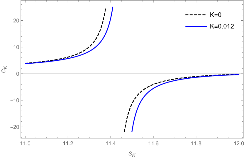
(a) For the range $11<S_{K}<12$

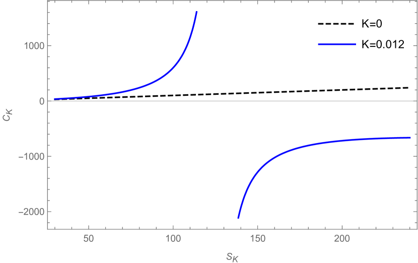
(b) For the range $20<S_{K}<250$

Figure 3: The heat capacity versus Kaniadakis entropy plots in the fixed $(J,\Phi)$ ensemble for $l=1,J=1$ and $\Phi=0.1$.

Fixed $(\Omega,Q)$ ensemble:

The modified mass for the Kaniadakis entropy case in the fixed $(\Omega,Q)$ ensemble is given by:

$$M_{K}^{\prime}=M_{K}-J\frac{\partial M_{K}}{\partial J}$$

where $\frac{\partial M_{K}}{\partial J}=\Omega$ is the angular velocity of the black hole with respect to the angular momentum J. By writing the term $M_{K}^{\prime}$ as $M_{K}$ for convenience we get:

$$M_{K}=\frac{\Omega^{2}}{16\pi^{2}}\left(\frac{K^{2}S_{K}^{4}}{\ln[KS_{K}+\sqrt{1+K^{2}S_{K}^{2}}]^{2}}-2S_{K}^{2}\right)+\frac{\pi Q^{2}}{2}\left(\ln\left[\frac{4\pi K}{\ln[KS_{K}+\sqrt{1+K^{2}S_{K}^{2}}]}\right]\right)+\frac{\ln[KS_{K}+\sqrt{1+K^{2}S_{K}^{2}}]^{2}}{16\pi^{2}K^{2}}$$ (21)

The heat capacity for the Kaniadakis entropy case in the fixed $(\Omega,Q)$ ensemble can be obtained as::

$$C_{K}=\frac{\frac{\partial M_{K}}{\partial S_{K}}}{\frac{\partial^{2}M_{K}}{\partial S_{K}^{2}}}\\ =-\frac{A}{B}$$

where,

$$A=(1+K^{2}S_{K}^{2})\ln(KS_{K}+\sqrt{1+K^{2}S_{K}^{2}})(4K^{2}\pi^{3}Q^{2}-\ln(KS_{K}+\sqrt{1+K^{2}S_{K}^{2}})^{2}+\Omega^{2}\ln(KS_{K}+\sqrt{1+K^{2}S_{K}^{2}})^{2})$$ (22)

and

$$B=K\biggl{(}4K^{2}\pi^{3}Q^{2}\sqrt{1+K^{2}S_{K}^{2}}+4K^{3}\pi^{3}Q^{2}S_{K}\ln(KS_{K}+\sqrt{1+K^{2}S_{K}^{2}})+\sqrt{1+K^{2}S_{K}^{2}}\ln(KS_{K}+\sqrt{1+K^{2}S_{K}^{2}})^{2}\\ -\sqrt{1+K^{2}S_{K}^{2}}\Omega^{2}\ln(KS_{K}+\sqrt{1+K^{2}S_{K}^{2}})^{2}-KS_{K}\ln(KS_{K}+\sqrt{1+K^{2}S_{K}^{2}})^{3}+KS_{K}\Omega^{2}\ln(KS_{K}+\sqrt{1+K^{2}S_{K}^{2}})^{3}\biggr{)}$$ (23)

In Fig.4 the heat capacity, $C_{K}$ is plotted against the Kaniadakis entropy, $S_{K}$ for $l=1,Q=2$ and $\Omega=0.2$ in the fixed $(\Omega,Q)$ ensemble. Here the solid blue curve represents the heat capacity for the Kaniadakis parameter, $K=0.012$ whereas the black dashed line represents the heat capacity for the Bekenstein-Hawking(BH) entropy case $(K=0)$. We find that for $K=0.012$, the heat capacity has a divergence at $S_{K}=138.16$ which indicates the presence of a Davies type phase transition present in the Kaniadakis modified black hole whereas the heat capacity for the BH entropy case shows no such behaviour.

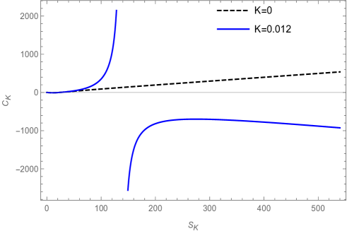
Figure 4: The heat capacity versus Kaniadakis entropy plot in the fixed $(\Omega,Q)$ ensemble for $l=1,Q=2$ and $\Omega=0.2$

III.2 The Renyi entropy case

The Renyi entropy, $S_{R}$ in terms of the black hole entropy, $S_{BH}$ is given by (5) as:

$$S_{R}=\frac{\ln[1+\lambda S_{BH}]}{\lambda}$$

where ‘$\lambda$’ is the Renyi parameter and for the limit $\lambda\rightarrow 0$, $S_{R}\rightarrow S_{BH}$. Starting with the above equation we get the modified horizon radius for the CR-BTZ black hole as:

$$S_{R}=\frac{\ln(1+4\pi\lambda r_{+})}{\lambda}$$

$$r_{+}=\frac{(e^{\lambda S_{R}}-1)}{4\pi\lambda}$$ (24)

We replace the horizon radius in (9) by the one obtained in (24) to get the modified mass $M_{R}$ for the CR-BTZ black hole which is given by :

$$M_{R}=\frac{4\pi^{2}\lambda^{2}J^{2}}{\left(e^{\lambda S_{R}}-1\right)^{2}}+\frac{\left(e^{\lambda S_{R}}-1\right)^{2}}{16\pi^{2}\lambda^{2}l^{2}}-\frac{\pi Q^{2}}{2}\ln\left[\frac{\left(e^{\lambda S_{R}}-1\right)}{4\pi\lambda}\right]$$

We compute and investigate the heat capacity of the charged rotating BTZ black hole for the case of Renyi entropy. We investigate the heat capacity for all the four thermodynamic ensembles namely: the fixed $(J,Q)$ ensemble, fixed $(\Omega,\Phi)$ ensemble, fixed $(J,\Phi)$ ensemble and the fixed $(\Omega,Q)$ ensemble.

We find that there are divergences in the heat capacity curves only for the fixed $(\Omega,\Phi)$ and the fixed $(J,\Phi)$ ensembles. The other two thermodynamic ensembles were found to show no such behaviour. We therefore present a detailed analysis of the heat capacity for the Renyi entropy case in the fixed $(\Omega,\Phi)$ and the fixed $(J,\Phi)$ ensembles as follows:

Fixed $(\Omega,\Phi)$ ensemble:

The modified mass for the Renyi entropy case in the fixed $(\Omega,\Phi)$ ensemble is given by:

$$M_{R}^{\prime}=M_{R}-J\frac{\partial M_{R}}{\partial J}-Q\frac{\partial M_{R}}{\partial Q}$$

$$M_{R}^{\prime}=M_{R}-J\Omega-Q\Phi$$

where $M_{R}^{\prime}$ is the modified mass for this ensemble and $\Omega$ and $\Phi$ are the angular velocity and electric potential of the black hole respectively. By making the necessary replacements and putting $l=1$, we get the final equation as follows:

$$M_{R}=\frac{-8\pi\lambda^{2}\Phi^{2}-\left(-1+e^{S_{R}\lambda}\right)^{2}\left(-1+\Omega^{2}\right)\ln(4\pi)+\left(-1+e^{S_{R}\lambda}\right)^{2}\left(-1+\Omega^{2}\right)\ln\left(\frac{-1+e^{S_{R}\lambda}}{\lambda}\right)}{16\pi^{2}\lambda^{2}\left(\ln\left(\frac{4\pi\lambda}{-1+e^{S_{R}\lambda}}\right)\right)}$$ (25)

We have here used the term $M_{R}$ instead of $M_{R}^{\prime}$ for convenience. Here $M_{R}$ is the modified mass for the fixed $(\Omega,\Phi)$ ensemble. The heat capacity for the Renyi entropy case in the fixed $(\Omega,\Phi)$ ensemble can be calculated as:

$$C_{R}=\frac{\frac{\partial M_{R}}{\partial S_{R}}}{\frac{\partial^{2}M_{R}}{\partial S_{R}^{2}}}\\ =-\frac{A}{B}$$

where,

$$A=(-1+e^{S_{R}\lambda})\biggl{(}\ln(4\pi)-\ln\bigg{(}\frac{-1+e^{S_{R}\lambda}}{\lambda}\bigg{)}\biggr{)}\biggl{(}4\pi\lambda^{2}\Phi^{2}+\left(-1+e^{S_{R}\lambda}\right)^{2}(-1+\Omega^{2})\ln(4\pi)^{2}+(-1+e^{S_{R}\lambda})^{2}(-1+\Omega^{2})\\ \ln\bigg{(}\frac{-1+e^{S_{R}\lambda}}{\lambda}\bigg{)}\ln\bigg{(}\frac{-1+e^{S_{R}\lambda}}{16\pi^{2}\lambda}\bigg{)}\biggr{)}$$ (26)

and

$$B=\lambda\biggl{(}4\pi\lambda^{2}\Phi^{2}\ln(4\pi)+(-1+\Omega^{2})\ln(4\pi)^{3}+5e^{2S_{R}\lambda}(-1+\Omega^{2})\ln(4\pi)^{3}-2e^{3S_{R}\lambda}(-1+\Omega^{2})\ln(4\pi)^{3}-4e^{S_{R}\lambda}\biggl{(}2\pi\lambda^{2}\Phi^{2}+\\ (-1+\Omega^{2})\ln(4\pi)^{3}\biggr{)}+\ln\bigg{(}\frac{-1+e^{S_{R}\lambda}}{\lambda}\bigg{)}\biggl{(}-4\pi\lambda^{2}\Phi^{2}+3(-1+e^{S_{R}\lambda})^{2}(-1+2e^{S_{R}\lambda})(-1+\Omega^{2})\ln(4\pi)^{2}+(-1+e^{S_{R}\lambda})^{2}(-1+2e^{S_{R}\lambda})\\ (-1+\Omega^{2})\ln\bigg{(}\frac{-1+e^{S_{R}\lambda}}{\lambda}\bigg{)}\ln\bigg{(}\frac{-1+e^{S_{R}\lambda}}{64\pi^{3}\lambda}\bigg{)}\biggr{)}\biggr{)}$$ (27)

We see from Fig.5(a) that the heat capacity, $C_{R}$ for the charged rotating BTZ black hole is plotted against the Renyi entropy, $S_{R}$ in the fixed $(\Omega,\Phi)$ ensemble. We see for $l=1,\Omega=0.2$ and $\Phi=0.1$ there are divergences in the heat capacity curve for both the Renyi and Bekenstein-Hawking (BH) entropy cases. These divergences refer to the presence of Davies type phase transitions in this thermodynamic ensemble. We find that the heat capacity has a divergence at $S_{R}=10.44$ for $\lambda=0.012$ as illustrated by the solid green curve. For the BH entropy case ($\lambda=0$) the divergence in the heat capacity is seen to occur at $S_{R}=11.08$ as depicted by the dashed curve in the figure.

Fixed $(J,\Phi)$ ensemble:

The modified mass for the Renyi entropy case in the fixed $(J,\Phi)$ ensemble is given by:

$$M_{R}^{\prime}=M_{R}-Q\frac{\partial M_{R}}{\partial Q}$$

$$M_{R}^{\prime}=M_{R}-Q\Phi$$

where $\frac{\partial M_{R}}{\partial Q}=\Phi$ is the electric potential of the black hole with respect to the electric charge Q. By making the necessary replacements and putting $l=1$, we get the final equation as follows:

$$M_{R}=\frac{1-2e^{S_{R}\lambda}+e^{2S_{R}\lambda}+\frac{64J^{2}\pi^{4}\lambda^{4}}{(-1+e^{S_{R}\lambda})^{2}}}{16\pi^{2}\lambda^{2}}+\frac{\Phi^{2}}{2\pi\ln\left(\frac{-1+e^{S_{R}\lambda}}{4\pi\lambda}\right)}$$ (28)

We have here used the term $M_{R}$ instead of $M_{R}^{\prime}$ for convenience. Here $M_{R}$ is the modified mass for the fixed $(J,\Phi)$ ensemble. The heat capacity for the Renyi entropy case in the fixed $(J,\Phi)$ ensemble can be calculated as:

$$C_{R}=\frac{\frac{\partial M_{R}}{\partial S_{R}}}{\frac{\partial^{2}M_{R}}{\partial S_{R}^{2}}}\\ =\frac{A}{B}$$

where,

$$A=(-1+e^{\lambda S_{R}})\left(\ln\left(\frac{4\pi\lambda}{-1+e^{\lambda S_{R}}}\right)\right)\biggl{(}-4(-1+e^{\lambda S_{R}})^{2}\pi\lambda^{2}\Phi^{2}+\left(-1+e^{\lambda S_{R}}\right)^{4}\ln(4\pi)^{2}-64J^{2}\pi^{4}\lambda^{4}\ln(4\pi)^{2}+\biggl{(}1-64J^{2}\pi^{4}\lambda^{4}\\ +e^{\lambda S_{R}}(-2+e^{\lambda S_{R}})(2-2e^{\lambda S_{R}}+e^{2\lambda S_{R}})\biggr{)}\ln\left(\frac{-1+e^{\lambda S_{R}}}{\lambda}\right)\left(-2\ln(4\pi)+\ln\left(\frac{-1+e^{\lambda S_{R}}}{\lambda}\right)\right)\biggr{)}$$ (29)

and

$$B=\lambda\biggl{(}4\pi\lambda^{2}\Phi^{2}\ln(4\pi)-9e^{4\lambda S_{R}}\ln(4\pi)^{3}+2e^{5\lambda S_{R}}\ln(4\pi)^{3}+(-1+64J^{2}\pi^{4}\lambda^{4})\ln(4\pi)^{3}+2e^{2\lambda S_{R}}\biggl{(}2\pi\lambda^{2}\Phi^{2}(4+\ln(4\pi))\\ -7\ln(4\pi)^{3}\biggr{)}-8e^{3\lambda S_{R}}\biggl{(}\pi\lambda^{2}\Phi^{2}-2\ln(4\pi)^{3}\biggr{)}+2e^{\lambda S_{R}}\biggl{(}-4\pi\lambda^{2}\Phi^{2}(1+\ln(4\pi))+(3+64J^{2}\pi^{4}\lambda^{4})\ln(4\pi)^{3}\biggr{)}+\ln\bigg{(}\frac{-1+e^{\lambda S_{R}}}{\lambda}\bigg{)}\\ \biggl{(}-4(-1+e^{\lambda S_{R}})^{2}\pi\lambda^{2}\Phi^{2}-3(-1+e^{\lambda S_{R}})^{4}(-1+2e^{\lambda S_{R}})\ln(4\pi)^{2}-192(1+2e^{\lambda S_{R}})J^{2}\pi^{4}\lambda^{4}\ln(4\pi)^{2}+\biggl{(}-1+64J^{2}\pi^{4}\lambda^{4}+\\ e^{\lambda S_{R}}\biggl{(}6-14e^{\lambda S_{R}}+16e^{2\lambda S_{R}}-9e^{3\lambda S_{R}}+2e^{4\lambda S_{R}}+128J^{2}\pi^{4}\lambda^{4}\biggr{)}\biggr{)}\biggl{(}3\ln(4\pi)-\ln\bigg{(}\frac{-1+e^{\lambda S_{R}}}{\lambda}\bigg{)}\biggr{)}\ln\bigg{(}\frac{-1+e^{\lambda S_{R}}}{\lambda}\bigg{)}\biggr{)}\biggr{)}$$ (30)

We see from Fig.5(b) that the heat capacity, $C_{R}$ for the charged rotating BTZ black hole is plotted against the Renyi entropy, $S_{R}$ in the fixed $(J,\Phi)$ ensemble. We see for $l=1,J=1$ and $\Phi=0.1$ there are divergences in the heat capacity curve for both the Renyi and Bekenstein-Hawking (BH) entropy cases. These divergences refer to the presence of Davies type phase transitions in this thermodynamic ensemble. We find that the heat capacity has a divergence at $S_{R}=10.71$ for $\lambda=0.012$ as illustrated by the solid green curve. For the BH entropy case ($\lambda=0$) the divergence in the heat capacity is seen to occur at $S_{R}=11.42$ as depicted by the dashed curve in the figure.

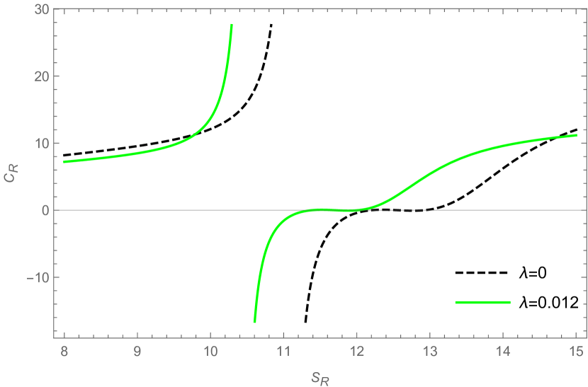
(a) Heat capacity in the fixed $(\Omega,\Phi)$ ensemble for $l=1,\Omega=0.2$ and $\Phi=0.1$

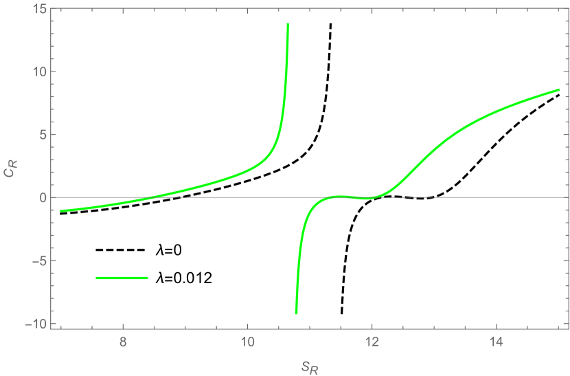
(b) Heat capacity in the fixed $(J,\Phi)$ ensemble for $l=1,J=1$ and $\Phi=0.1$.

Figure 5: The heat capacity versus Renyi entropy plots in the fixed $(\Omega,\Phi)$ and fixed $(J,\Phi)$ ensembles.

III.3 The Sharma-Mittal entropy case

The Sharma-Mittal entropy, $S_{SM}$ in terms of the black hole entropy, $S_{BH}$ is given by (6) as:

$$S_{SM}=\frac{\left[\left(1+\lambda S_{BH}\right)^{\frac{\rho}{\lambda}}-1\right]}{\rho}$$

where ‘$\rho$’ here is the new free parameter and for the limit $\rho\rightarrow\lambda$, $S_{SM}\rightarrow S_{BH}$. Starting with the above equation we get the modified horizon radius for the CR-BTZ black hole as:

$$S_{SM}=\frac{\left[\left(1+4\pi\lambda r_{+}\right)^{\frac{\rho}{\lambda}}-1\right]}{\rho}$$

$$r_{+}=\frac{(\rho S_{SM}+1)^{\frac{\lambda}{\rho}}-1}{\lambda}$$ (31)

We replace the horizon radius in (9) by the one obtained in (31) to get the modified mass $M_{SM}$ for the CR-BTZ black hole which is given by :

$$M_{SM}=\frac{4\pi^{2}\lambda^{2}J^{2}}{\left[(\rho S_{SM}+1)^{\left(\frac{\lambda}{\rho}\right)}-1\right]^{2}}+\frac{\left[(\rho S_{SM}+1)^{\left(\frac{\lambda}{\rho}\right)}-1\right]^{2}}{16\pi^{2}\lambda^{2}l^{2}}-\frac{\pi Q^{2}}{2}Log\left[\frac{\left[(\rho S_{SM}+1)^{\left(\frac{\lambda}{\rho}\right)}-1\right]}{4\pi\lambda}\right]$$

We compute and investigate the heat capacity of the charged rotating BTZ black hole for the case of Sharma-Mittal entropy. We investigate the heat capacity for all the four thermodynamic ensembles namely: the fixed $(J,Q)$ ensemble, fixed $(\Omega,\Phi)$ ensemble, fixed $(J,\Phi)$ ensemble and the fixed $(\Omega,Q)$ ensemble.

We find that there are divergences in the heat capacity curves only for the fixed $(\Omega,\Phi)$ and the fixed $(J,\Phi)$ ensembles. The other two thermodynamic ensembles were found to show no such behaviour. We therefore present a detailed analysis of the heat capacity for the Sharma-Mittal entropy case in the fixed $(\Omega,\Phi)$ and the fixed $(J,\Phi)$ ensembles as follows:

Fixed $(\Omega,\Phi)$ ensemble:

The modified mass for the Sharma-Mittal entropy case in the fixed $(\Omega,\Phi)$ ensemble is given by:

$$M_{SM}^{\prime}=M_{SM}-J\frac{\partial M_{SM}}{\partial J}-Q\frac{\partial M_{SM}}{\partial Q}$$

$$M_{SM}^{\prime}=M_{SM}-J\Omega-Q\Phi$$

where $M_{SM}^{\prime}$ is the modified mass for this ensemble and $\Omega$ and $\Phi$ are the angular velocity and electric potential of the black hole respectively. By making the necessary replacements and putting $l=1$, we get the final equation as follows:

$$M_{SM}=\frac{\mathcal{X}}{\mathcal{Y}}$$ (32)

where,

$$\mathcal{X}=\bigl{(}-8\pi\lambda^{2}\Phi^{2}-(-1+(1+\rho S_{SM})^{\lambda/\rho})^{2}(-1+\Omega^{2})\ln[4\pi]+(-1+(1+\rho S_{SM})^{\lambda/\rho})^{2}(-1+\Omega^{2})\\ \ln\bigg{(}(-1+(1+\rho S_{SM})^{\lambda/\rho})/\lambda\bigg{)}\biggr{)}$$ (33)

and

$$\mathcal{Y}=16\pi^{2}\lambda^{2}\ln\left(\frac{4\pi\lambda}{-1+(1+\rho S_{SM})^{\lambda/\rho}}\right)$$ (34)

We have here used the term $M_{SM}$ instead of $M_{SM}^{\prime}$ for convenience. Here $M_{SM}$ is the modified mass for the fixed $(\Omega,\Phi)$ ensemble. The heat capacity for the Sharma-Mittal entropy case in the fixed $(\Omega,\Phi)$ ensemble can be calculated as:

$$C_{SM}=-\frac{A}{B}$$

where,

$$A=\biggl{(}(1+\rho S_{SM})\biggl{(}-1+(1+\rho S_{SM})^{\frac{\lambda}{\rho}}\biggr{)}\biggl{(}\ln[4\pi]-\ln\bigg{(}\frac{-1+(1+\rho S_{SM})^{\frac{\lambda}{\rho}}}{\lambda}\bigg{)}\biggr{)}\biggl{(}4\pi\lambda^{2}\Phi^{2}+\biggl{(}-1+(1+\rho S_{SM})^{\frac{\lambda}{\rho}}\biggr{)}^{2}\biggl{(}-1+\Omega^{2}\biggr{)}\\ \ln[4\pi]^{2}+\biggl{(}-1+(1+\rho S_{SM})^{\frac{\lambda}{\rho}}\biggr{)}^{2}\biggl{(}-1+\Omega^{2}\biggr{)}\ln\bigg{(}\frac{-1+(1+\rho S_{SM})^{\frac{\lambda}{\rho}}}{16\pi^{2}\lambda}\bigg{)}\biggr{)}\biggr{)}$$ (35)

and

$$B=\biggl{(}-1+(1+\rho S_{SM})^{\frac{\lambda}{\rho}}\biggr{)}^{2}\biggl{(}\lambda-\rho+(-2\lambda+\rho)(1+\rho S_{SM})^{\frac{\lambda}{\rho}}\biggr{)}\biggl{(}-1+\Omega^{2}\biggr{)}\ln[4\pi]^{3}+4\pi\lambda^{2}\Phi^{2}\biggl{(}(\lambda-\rho)\ln[4\pi]+(1+\rho S_{SM})^{\frac{\lambda}{\rho}}(-2\lambda+\rho)\\ \ln[4\pi]\biggr{)}+\ln\bigg{(}\frac{-1+(1+\rho S_{SM})^{\frac{\lambda}{\rho}}}{\lambda}\bigg{)}\biggl{(}-4\pi\lambda^{2}\biggl{(}\lambda+\rho\biggl{(}-1+(1+\rho S_{SM})^{\frac{\lambda}{\rho}}\biggr{)}\biggr{)}\Phi^{2}-3\biggl{(}-1+(1+\rho S_{SM})^{\frac{\lambda}{\rho}}\biggr{)}^{2}\biggl{(}\lambda-\rho+(-2\lambda+\rho)\\ (1+\rho S_{SM})^{\frac{\lambda}{\rho}}\biggr{)}\biggl{(}-1+\Omega^{2}\biggr{)}\ln[4\pi]^{2}+\biggl{(}-1+(1+\rho S_{SM})^{\frac{\lambda}{\rho}}\biggr{)}^{2}\biggl{(}-\lambda+\rho+(2\lambda-\rho)(1+\rho S_{SM})^{\frac{\lambda}{\rho}}\biggr{)}\biggl{(}-1+\Omega^{2}\biggr{)}\ln\bigg{(}\frac{-1+(1+\rho S_{SM})^{\frac{\lambda}{\rho}}}{\lambda}\bigg{)}\\ \biggl{(}-3\ln[4\pi]+\ln\bigg{(}\frac{-1+(1+\rho S_{SM})^{\frac{\lambda}{\rho}}}{\lambda}\bigg{)}\biggr{)}\biggr{)}$$ (36)

We see from Fig.6(a) that the heat capacity, $C_{SM}$ for the charged rotating BTZ black hole is plotted against the Sharma-Mittal entropy, $S_{SM}$ in the fixed $(\Omega,\Phi)$ ensemble. We see for $l=1,\Omega=0.2$ and $\Phi=0.1$ there are divergences in the heat capacity curve for both the Sharma-Mittal and Bekenstein-Hawking (BH) entropy cases. These divergences refer to the presence of Davies type phase transitions in this thermodynamic ensemble. We find that the heat capacity has a divergence at $S_{SM}=12.32$ for $\lambda=0.67\rho$ as illustrated by the solid orange curve. For the BH entropy case ($\lambda=\rho$) the divergence in the heat capacity is seen to occur at $S_{SM}=11.08$ as depicted by the dashed curve in the figure.

Fixed $(J,\Phi)$ ensemble:

The modified mass for the Sharma-Mittal entropy case in the fixed $(J,\Phi)$ ensemble is given by:

$$M_{SM}^{\prime}=M_{SM}-Q\frac{\partial M_{SM}}{\partial Q}$$

$$M_{SM}^{\prime}=M_{SM}-Q\Phi$$

where $\frac{\partial M_{SM}}{\partial Q}=\Phi$ is the electric potential of the black hole with respect to the electric charge Q. By making the necessary replacements and putting $l=1$, we get the final equation as follows:

$$M_{SM}=\frac{\left(\left(\frac{64J^{2}\pi^{4}\lambda^{4}}{(-1+(1+\rho S_{SM})^{\lambda/\rho})^{2}}+(-1+(1+\rho S_{SM})^{\lambda/\rho})^{2}+\frac{8\pi\lambda^{2}\Phi^{2}}{\ln{\left(\frac{-1+(1+\rho S_{SM})^{\lambda/\rho}}{4\pi\lambda}\right)}}\right)\right)}{16\pi^{2}\lambda^{2}}$$ (37)

We have here used the term $M_{SM}$ instead of $M_{SM}^{\prime}$ for convenience. Here $M_{SM}$ is the modified mass for the fixed $(J,\Phi)$ ensemble. The heat capacity for the Sharma-Mittal entropy case in the fixed $(J,\Phi)$ ensemble can be calculated as:

$$C_{SM}=\frac{\frac{\partial M_{SM}}{\partial S_{SM}}}{\frac{\partial^{2}M_{SM}}{\partial S_{SM}^{2}}}\\ =-\frac{A}{B}$$

where,

$$A=\biggl{(}\biggl{(}1+\rho S_{SM}\biggr{)}\biggl{(}-1+(1+\rho S_{SM})^{\frac{\lambda}{\rho}}\biggr{)}\biggl{(}-\ln\bigg{(}\frac{-1+(1+\rho S_{SM})^{\frac{\lambda}{\rho}}}{4\pi\lambda}\bigg{)}\biggr{)}\\ \biggl{(}-4\pi\lambda^{2}\biggl{(}-1+(1+\rho S_{SM})^{\frac{\lambda}{\rho}}\biggr{)}^{2}\Phi^{2}-64J^{2}\pi^{4}\lambda^{4}\ln[4\pi]^{2}\\ +\biggl{(}-1+(1+\rho S_{SM})^{\frac{\lambda}{\rho}}\biggr{)}^{4}\ln[4\pi]^{2}\\ +\biggl{(}-64J^{2}\pi^{4}\lambda^{4}+\biggl{(}-1+(1+\rho S_{SM})^{\frac{\lambda}{\rho}}\biggr{)}^{4}\biggr{)}\ln\bigg{(}\frac{-1+(1+\rho S_{SM})^{\frac{\lambda}{\rho}}}{\lambda}\bigg{)}\\ \biggl{(}-2\ln[4\pi]+\ln\bigg{(}\frac{-1+(1+\rho S_{SM})^{\frac{\lambda}{\rho}}}{\lambda}\bigg{)}\biggr{)}\biggr{)}$$ (38)

and

$$B=\biggl{(}\biggl{(}-1+\biggl{(}1+\rho S_{SM}\biggr{)}^{\frac{\lambda}{\rho}}\biggr{)}^{4}(\lambda-\rho+(-2\lambda+\rho)(1+\rho S_{SM})^{\frac{\lambda}{\rho}})\ln[4\pi]^{3}\\ -64J^{2}\pi^{4}\lambda^{4}(\lambda-\rho+(2\lambda+\rho)(1+\rho S_{SM})^{\frac{\lambda}{\rho}})\ln[4\pi]^{3}\\ +4\pi\lambda^{2}\biggl{(}-1+(1+\rho S_{SM})^{\frac{\lambda}{\rho}}\biggr{)}^{2}\Phi^{2}\biggl{(}(-\lambda+\rho)\ln[4\pi]\\ +(1+\rho S_{SM})^{\frac{\lambda}{\rho}}(2\lambda-\rho)\ln[4\pi]\biggr{)}\\ +\ln\bigg{(}\frac{-1+(1+\rho S_{SM})^{\frac{\lambda}{\rho}}}{\lambda}\bigg{)}\biggl{(}4\pi\lambda^{2}\biggl{(}-1+(1+\rho S_{SM})^{\frac{\lambda}{\rho}}\biggr{)}^{2}\\ \biggl{(}\lambda+\rho\biggl{(}-1+(1+\rho S_{SM})^{\frac{\lambda}{\rho}}\biggr{)}\biggr{)}\Phi^{2}\\ -3\biggl{(}-1+(1+\rho S_{SM})^{\frac{\lambda}{\rho}}\biggr{)}^{4}(\lambda-\rho+(-2\lambda+\rho)(1+\rho S_{SM})^{\frac{\lambda}{\rho}})\ln[4\pi]^{2}\\ +192J^{2}\pi^{4}\lambda^{4}(\lambda-\rho+(2\lambda+\rho)(1+\rho S_{SM})^{\frac{\lambda}{\rho}})\ln[4\pi]^{2}\\ +\biggl{(}64J^{2}\pi^{4}\lambda^{4}\rho\biggl{(}-1+(1+\rho S_{SM})^{\frac{\lambda}{\rho}}\biggr{)}-\rho\biggl{(}-1+(1+\rho S_{SM})^{\frac{\lambda}{\rho}}\biggr{)}^{5}\\ +\lambda\biggl{(}-1+(1+\rho S_{SM})^{\frac{\lambda}{\rho}}\biggr{)}^{4}\biggl{(}-1+2\biggl{(}1+\rho S_{SM}\biggr{)}^{\frac{\lambda}{\rho}}\biggr{)}\\ +64J^{2}\pi^{4}\lambda^{5}\biggl{(}1+2\biggl{(}1+\rho S_{SM}\biggr{)}^{\frac{\lambda}{\rho}}\biggr{)}\biggr{)}\\ \ln\bigg{(}\frac{-1+(1+\rho S_{SM})^{\frac{\lambda}{\rho}}}{\lambda}\bigg{)}\biggl{(}-3\ln[4\pi]\\ +\ln\bigg{(}\frac{-1+(1+\rho S_{SM})^{\frac{\lambda}{\rho}}}{\lambda}\bigg{)}\biggr{)}\biggr{)}$$ (39)

We see from Fig.6(b) that the heat capacity, $C_{SM}$ for the charged rotating BTZ black hole is plotted against the Sharma-Mittal entropy, $S_{SM}$ in the fixed $(J,\Phi)$ ensemble. We see for $l=1,J=1$ and $\Phi=0.1$ there are divergences in the heat capacity curve for both the Sharma-Mittal and Bekenstein-Hawking (BH) entropy cases. These divergences refer to the presence of Davies type phase transitions in this thermodynamic ensemble. We find that the heat capacity has a divergence at $S_{SM}=12.84$ for $\lambda=0.67\rho$ as illustrated by the solid orange curve. For the BH entropy case ($\lambda=\rho$) the divergence in the heat capacity is seen to occur at $S_{SM}=11.42$ as depicted by the dashed curve in the figure.

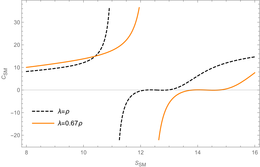
(a) Heat capacity in the fixed $(\Omega,\Phi)$ ensemble for $l=1,\Omega=0.2$ and $\Phi=0.1$.

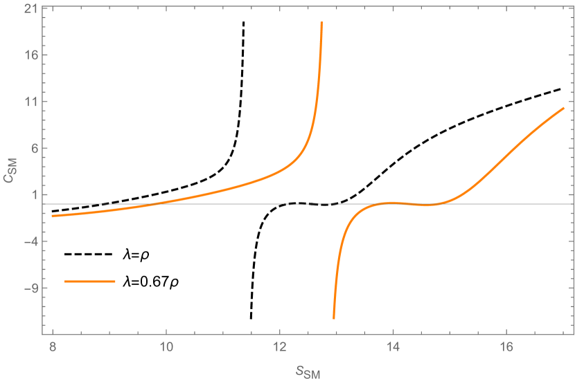
(b) Heat capacity in the fixed $(J,\Phi)$ ensemble for $l=1,J=1$ and $\Phi=0.1$.

Figure 6: The heat capacity versus Sharma-Mittal entropy plots in the fixed $(\Omega,\Phi)$ and fixed $(J,\Phi)$ ensembles.

III.4 The Tsallis-Cirto entropy case

The Tsallis-Cirto entropy, $S_{\delta}$ in terms of the black hole entropy, $S_{BH}$ is given by (7) as:

$$S_{\delta}=(S_{BH})^{\delta}$$

where ‘$\delta$’ is a real parameter and for the limit $\delta\rightarrow 1$, $S_{\delta}\rightarrow S_{BH}$. Starting with the above equation we get the modified horizon radius for the CR-BTZ black hole as:

$$S_{\delta}=(4\pi r_{+})^{\delta}$$

$$r_{+}=\frac{S_{\delta}^{\frac{1}{\delta}}}{4\pi}$$ (40)

We replace the horizon radius in (9) by the one obtained in (40) to get the modified mass $M_{\delta}$ for the CR-BTZ black hole which is given by :

$$M_{\delta}=\frac{4\pi^{2}J^{2}}{S_{\delta}^{\frac{2}{\delta}}}+\frac{S_{\delta}^{\frac{2}{\delta}}}{16\pi^{2}l^{2}}-\frac{\pi Q^{2}}{2}Log\left[\frac{S_{\delta}^{\frac{1}{\delta}}}{4\pi}\right]$$

We compute and investigate the heat capacity of the charged rotating BTZ black hole for the case of Tsallis-Cirto entropy. We investigate the heat capacity for all the four thermodynamic ensembles namely: the fixed $(J,Q)$ ensemble, fixed $(\Omega,\Phi)$ ensemble, fixed $(J,\Phi)$ ensemble and the fixed $(\Omega,Q)$ ensemble.

We find that there are divergences in the heat capacity curves only for the fixed $(\Omega,\Phi)$ and the fixed $(J,\Phi)$ ensembles. The other two thermodynamic ensembles were found to show no such behaviour. We therefore present a detailed analysis of the heat capacity for the Tsallis-Cirto entropy case in the fixed $(\Omega,\Phi)$ and the fixed $(J,\Phi)$ ensembles as follows:

Fixed $(\Omega,\Phi)$ ensemble:

The modified mass for the Tsallis-Cirto entropy case in the fixed $(\Omega,\Phi)$ ensemble is given by:

$$M_{\delta}^{\prime}=M_{\delta}-J\frac{\partial M_{\delta}}{\partial J}-Q\frac{\partial M_{\delta}}{\partial Q}$$

$$M_{\delta}^{\prime}=M_{\delta}-J\Omega-Q\Phi$$

where $M_{\delta}^{\prime}$ is the modified mass for this ensemble and $\Omega$ and $\Phi$ are the angular velocity and electric potential of the black hole respectively. By making the necessary replacements and putting $l=1$, we get the final equation as follows:

$$M_{\delta}=\frac{-8\pi\Phi^{2}+S_{\delta}^{\frac{2}{\delta}}(-1+\Omega^{2})\ln\left(\frac{S_{\delta}^{\frac{1}{\delta}}}{4\pi}\right)}{16\pi^{2}\left(\ln(4\pi)-\ln\left(S_{\delta}^{\frac{1}{\delta}}\right)\right)}$$ (41)

We have here used the term $M_{\delta}$ instead of $M_{\delta}^{\prime}$ for convenience. Here $M_{\delta}$ is the modified mass for the fixed $(\Omega,\Phi)$ ensemble. The heat capacity for the Tsallis-Cirto entropy case in the fixed $(\Omega,\Phi)$ ensemble can be calculated as:

$$C_{\delta}=\frac{\frac{\partial M_{\delta}}{\partial S_{\delta}}}{\frac{\partial^{2}M_{\delta}}{\partial S_{\delta}^{2}}}=\frac{S\delta}{2-\delta+\frac{8\pi\Phi^{2}\left(1-\ln(4\pi)+\ln\left(S^{\frac{1}{\delta}}\right)\right)}{\left(\ln(4\pi)-\ln\left(S^{\frac{1}{\delta}}\right)\right)\left(4\pi\Phi^{2}+S^{\frac{2}{\delta}}(-1+\Omega^{2})\ln^{2}\left(\frac{S^{\frac{1}{\delta}}}{4\pi}\right)\right)}}$$ (42)

We see from Fig.7(a) that the heat capacity, $C_{\delta}$ for the charged rotating BTZ black hole is plotted against the Tsallis-Cirto entropy, $S_{\delta}$ in the fixed $(\Omega,\Phi)$ ensemble. We see for $l=1,\Omega=0.2$ and $\Phi=0.1$ there are divergences in the heat capacity curve for both the Tsallis-Cirto and Bekenstein-Hawking (BH) entropy cases. These divergences refer to the presence of Davies type phase transitions in this thermodynamic ensemble. We find that the heat capacity has a divergence at $S_{\delta}=14.69$ for $\delta=1.12$ as illustrated by the solid purple curve. For the BH entropy case ($\delta=1$) the divergence in the heat capacity is seen to occur at $S_{\delta}=11.08$ as depicted by the dashed curve in the figure.

Fixed $(J,\Phi)$ ensemble:

The modified mass for the Tsallis-Cirto entropy case in the fixed $(J,\Phi)$ ensemble is given by:

$$M_{\delta}^{\prime}=M_{\delta}-Q\frac{\partial M_{\delta}}{\partial Q}$$

$$M_{\delta}^{\prime}=M_{\delta}-Q\Phi$$

where $\frac{\partial M_{\delta}}{\partial Q}=\Phi$ is the electric potential of the black hole with respect to the electric charge Q. By making the necessary replacements and putting $l=1$, we get the final equation as follows:

$$M_{\delta}=\frac{64J^{2}\pi^{4}S^{-\frac{2}{\delta}}+S^{\frac{2}{\delta}}+\frac{8\pi\Phi^{2}}{\ln\left(\frac{S^{\frac{1}{\delta}}}{4\pi}\right)}}{16\pi^{2}}$$ (43)

We have here used the term $M_{\delta}$ instead of $M_{\delta}^{\prime}$ for convenience. Here $M_{\delta}$ is the modified mass for the fixed $(J,\Phi)$ ensemble. The heat capacity for the Tsallis-Cirto entropy case in the fixed $(J,\Phi)$ ensemble can be calculated as:

$$C_{\delta}=\frac{\frac{\partial M_{\delta}}{\partial S_{\delta}}}{\frac{\partial^{2}M_{\delta}}{\partial S_{\delta}^{2}}}\\ =\frac{S\delta(\ln(4\pi)-\ln(S^{1/\delta}))\left(4\pi S^{2/\delta}\Phi^{2}-(-64J^{2}\pi^{4}+S^{4/\delta})\ln\left(\frac{S^{1/\delta}}{4\pi}\right)^{2}\right)}{S^{4/\delta}(-2+\delta)(\ln(4\pi)-\ln(S^{1/\delta}))^{3}+4\pi S^{2/\delta}\Phi^{2}(2-\delta\ln(4\pi)+\delta\ln(S^{1/\delta}))+64J^{2}\pi^{4}(2+\delta)\log\left(\frac{S^{1/\delta}}{4\pi}\right)^{3}}$$

We see from Fig.7(b) that the heat capacity, $C_{\delta}$ for the charged rotating BTZ black hole is plotted against the Tsallis-Cirto entropy, $S_{\delta}$ in the fixed $(J,\Phi)$ ensemble. We see for $l=1,J=1$ and $\Phi=0.1$ there are divergences in the heat capacity curve for both the Tsallis-Cirto and Bekenstein-Hawking (BH) entropy cases. These divergences refer to the presence of Davies type phase transitions in this thermodynamic ensemble. We find that the heat capacity has a divergence at $S_{\delta}=15.28$ for $\delta=1.12$ as illustrated by the solid purple curve. For the BH entropy case ($\delta=1$) the divergence in the heat capacity is seen to occur at $S_{\delta}=11.42$ as depicted by the dashed curve in the figure.

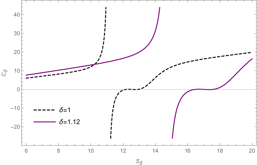
(a) Heat capacity in the fixed $(\Omega,\Phi)$ ensemble for $l=1,\Omega=0.2$ and $\Phi=0.1$.

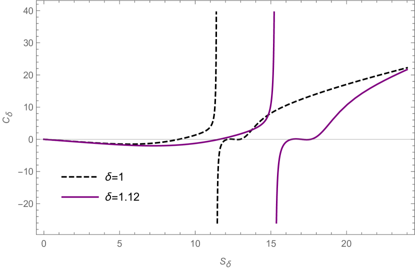
(b) Heat capacity in the fixed $(J,\Phi)$ ensemble for $l=1,J=1$ and $\Phi=0.1$.

Figure 7: The heat capacity versus Tsallis-Cirto entropy plots in the fixed $(\Omega,\Phi)$ and fixed $(J,\Phi)$ ensembles.

III.5 The Barrow entropy case

The Barrow entropy, $S_{\Delta}$ in terms of the black hole entropy, $S_{BH}$ is given by (8) as:

$$S_{\Delta}=(S_{BH})^{1+\Delta/2}$$

where, ‘$\Delta$’ is the parameter that is linked to the fractal structure of the system and for the limit $\Delta\rightarrow 0$, $S_{\Delta}\rightarrow S_{BH}$. Starting with the above equation we get the modified horizon radius for the CR-BTZ black hole as:

$$S_{\Delta}=(4\pi r_{+})^{1+\Delta/2}$$

$$r_{+}=\frac{S_{\Delta}^{\frac{2}{2+\Delta}}}{4\pi}$$ (44)

We replace the horizon radius in (9) by the one obtained in (44) to get the modified mass $M_{\Delta}$ for the CR-BTZ black hole which is given by :

$$M_{\Delta}=4J^{2}\pi^{2}S^{-\left(\frac{4}{2+\Delta}\right)}+\left(\frac{S^{\left(\frac{4}{2+\Delta}\right)}}{16\pi^{2}}\right)+\frac{1}{2}\pi Q^{2}\left(\ln\left(\frac{4\pi}{S^{\frac{2}{2+\Delta}}}\right)\right)$$

We compute and investigate the heat capacity of the charged rotating BTZ black hole for the case of Barrow entropy. We investigate the heat capacity for all the four thermodynamic ensembles namely: the fixed $(J,Q)$ ensemble, fixed $(\Omega,\Phi)$ ensemble, fixed $(J,\Phi)$ ensemble and the fixed $(\Omega,Q)$ ensemble.

We find that there are divergences in the heat capacity curves only for the fixed $(\Omega,\Phi)$ and the fixed $(J,\Phi)$ ensembles. The other two thermodynamic ensembles were found to show no such behaviour. We therefore present a detailed analysis of the heat capacity for the Barrow entropy case in the fixed $(\Omega,\Phi)$ and the fixed $(J,\Phi)$ ensembles as follows:

Fixed $(\Omega,\Phi)$ ensemble:

The modified mass for the Barrow entropy case in the fixed $(\Omega,\Phi)$ ensemble is given by:

$$M_{\Delta}^{\prime}=M_{\Delta}-J\frac{\partial M_{\Delta}}{\partial J}-Q\frac{\partial M_{\Delta}}{\partial Q}$$

$$M_{\Delta}^{\prime}=M_{\Delta}-J\Omega-Q\Phi$$

where $M_{\Delta}^{\prime}$ is the modified mass for this ensemble and $\Omega$ and $\Phi$ are the angular velocity and electric potential of the black hole respectively. By making the necessary replacements and putting $l=1$, we get the final equation as follows:

$$M_{\Delta}=\frac{-8\pi\Phi^{2}+S^{\frac{4}{2+\Delta}}\left(-1+\Omega^{2}\right)\ln{\left(\frac{S^{\frac{2}{2+\Delta}}}{4\pi}\right)}}{16\pi^{2}\left(\ln{4\pi}-\ln{S^{\frac{2}{2+\Delta}}}\right)}$$ (45)

We have here used the term $M_{\Delta}$ instead of $M_{\Delta}^{\prime}$ for convenience. Here $M_{\Delta}$ is the modified mass for the fixed $(\Omega,\Phi)$ ensemble. The heat capacity for the Barrow entropy case in the fixed $(\Omega,\Phi)$ ensemble can be calculated as:

$$C_{\Delta}=\frac{\frac{\partial M_{\Delta}}{\partial S_{\Delta}}}{\frac{\partial^{2}M_{\Delta}}{\partial S_{\Delta}^{2}}}\\ =\frac{S(2+\Delta)}{2-\Delta+\frac{16\pi\Phi^{2}\left(1-\ln{4\pi}+\ln{S^{\frac{2}{2+\Delta}}}\right)}{\left(\ln{4\pi}-\ln{S^{\frac{2}{2+\Delta}}}\right)\left(4\pi\Phi^{2}+S^{\frac{4}{2+\Delta}}\left(-1+\Omega^{2}\right)\ln{\left(\frac{S^{\frac{2}{2+\Delta}}}{4\pi}\right)^{2}}\right)}}$$

We see from Fig.8(a) that the heat capacity, $C_{\Delta}$ for the charged rotating BTZ black hole is plotted against the Barrow entropy, $S_{\Delta}$ in the fixed $(\Omega,\Phi)$ ensemble. We see for $l=1,\Omega=0.2$ and $\Phi=0.1$ there are divergences in the heat capacity curve for both the Barrow and Bekenstein-Hawking (BH) entropy cases. These divergences refer to the presence of Davies type phase transitions in this thermodynamic ensemble. We find that the heat capacity has a divergence at $S_{\Delta}=12.76$ for $\Delta=0.12$ as illustrated by the solid red curve. For the BH entropy case ($\Delta=0$) the divergence in the heat capacity is seen to occur at $S_{\Delta}=11.08$ as depicted by the dashed curve in the figure.

Fixed $(J,\Phi)$ ensemble:

The modified mass for the Barrow entropy case in the fixed $(J,\Phi)$ ensemble is given by:

$$M_{\Delta}^{\prime}=M_{\Delta}-Q\frac{\partial M_{\Delta}}{\partial Q}$$

$$M_{\Delta}^{\prime}=M_{\Delta}-Q\Phi$$

where $\frac{\partial M_{\Delta}}{\partial Q}=\Phi$ is the electric potential of the black hole with respect to the electric charge Q. By making the necessary replacements and putting $l=1$, we get the final equation as follows:

$$M_{\Delta}=\frac{64J^{2}\pi^{4}S^{-\frac{4}{2+\Delta}}+S^{\frac{4}{2+\Delta}}+\frac{8\pi\Phi^{2}}{\log\left(\frac{S^{\frac{2}{2+\Delta}}}{4\pi}\right)}}{16\pi^{2}}$$ (46)

We have here used the term $M_{\delta}$ instead of $M_{\delta}^{\prime}$ for convenience. Here $M_{\delta}$ is the modified mass for the fixed $(J,\Phi)$ ensemble. The heat capacity for the Tsallis-Cirto entropy case in the fixed $(J,\Phi)$ ensemble can be calculated as:

$$C_{\Delta}=\frac{\frac{\partial M_{\Delta}}{\partial S_{\Delta}}}{\frac{\partial^{2}M_{\Delta}}{\partial S_{\Delta}^{2}}}\\ =\frac{S(2+\Delta)\ln\left(\frac{4\pi}{S^{\frac{2}{2+\Delta}}}\right)\left(4\pi S^{\frac{4}{2+\Delta}}\Phi^{2}-(-64J^{2}\pi^{4}+S^{\frac{8}{2+\Delta}})\ln\left(\frac{S^{\frac{2}{2+\Delta}}}{4\pi}\right)^{2}\right)}{S^{\frac{8}{2+\Delta}}\left(\ln\left(\frac{4\pi}{S^{\frac{2}{2+\Delta}}}\right)\right)^{3}+4\pi S^{\frac{4}{2+\Delta}}\Phi^{2}(4-(2+\Delta)\ln(4\pi)+(2+\Delta)\ln(S^{\frac{2}{2+\Delta}}))+64J^{2}\pi^{4}(6+\Delta)\ln\left(\frac{S^{\frac{2}{2+\Delta}}}{4\pi}\right)^{3}}$$

We see from Fig.8(b) that the heat capacity, $C_{\Delta}$ for the charged rotating BTZ black hole is plotted against the Barrow entropy, $S_{\Delta}$ in the fixed $(J,\Phi)$ ensemble. We see for $l=1,J=1$ and $\Phi=0.1$ there are divergences in the heat capacity curve for both the Barrow and Bekenstein-Hawking (BH) entropy cases. These divergences refer to the presence of Davies type phase transitions in this thermodynamic ensemble. We find that the heat capacity has a divergence at $S_{\Delta}=13.21$ for $\Delta=0.12$ as illustrated by the solid red curve. For the BH entropy case ($\Delta=0$) the divergence in the heat capacity is seen to occur at $S_{\Delta}=11.42$ as depicted by the dashed curve in the figure.

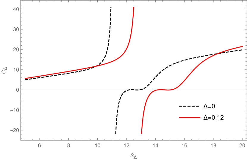
(a) Heat capacity in the fixed $(\Omega,\Phi)$ ensemble for $l=1,\Omega=0.2$ and $\Phi=0.1$.

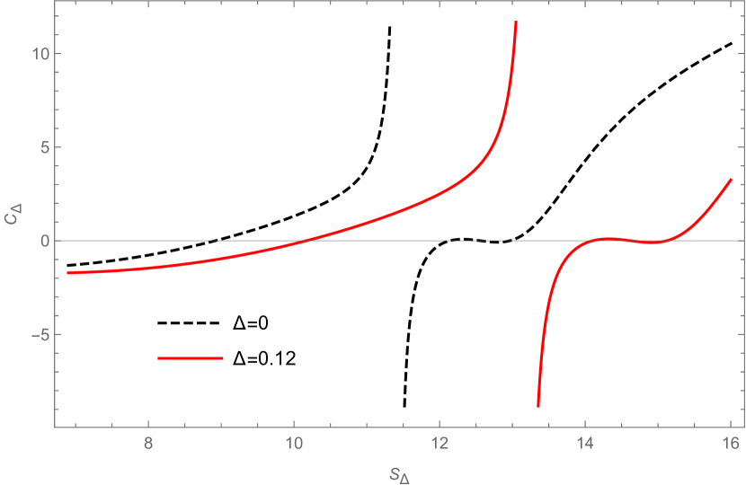
(b) Heat capacity in the fixed $(J,\Phi)$ ensemble for $l=1,J=1$ and $\Phi=0.1$.

Figure 8: The heat capacity versus Barrow entropy plots in the fixed $(\Omega,\Phi)$ and fixed $(J,\Phi)$ ensembles.

IV Thermodynamic geometry of the CR-BTZ black hole

We discuss the thermodynamic geometry of the charged rotating BTZ black hole for both the Ruppeiner and geometrothermodynamic (GTD) formalisms. The Ruppeiner metric is defined as the negative hessian of entropy with respect to other extensive variables. Therefore it is only the fixed $(J,Q)$ ensemble which holds good in the Ruppeiner formalism as both $J$ and $Q$ are extensive thermodynamic quantities.

The other thermodynamic ensembles namely: the fixed $(\Omega,\Phi)$ ensemble, fixed $(J,\Phi)$ ensemble and the fixed $(\Omega,Q)$ ensemble comprise of intensive variables like $\Omega$ and $\Phi$ which are the angular velocity and electric potential of the charged rotating BTZ black hole respectively. Therefore these thermodynamic ensembles do not hold good as per the definition of the Ruppeiner metric. We therefore discuss the thermodynamic geometry of all these ensembles in the GTD formalism which is defined on a multi-dimensional phase space that comprises of both the extensive and intensive variables of the thermodynamic system. The GTD formalism is therefore the appropriate geometric formalism for discussing all the thermodynamic ensembles.

We first discuss the Ruppeiner geometry of the charged rotating BTZ black hole in the fixed $(J,Q)$ ensemble where we observe a curvature singularity in the Ruppeiner scalar curve only for the Kaniadakis entropy case. We then discuss the GTD geometry of the black hole for all the thermodynamic ensembles, where we observe curvature singularities in the GTD scalar curves for all the non-extensive entropy cases. These curvature singularities are seen to occur exactly at the points where we saw divergences in the corresponding heat capacity curves in the previous section.

IV.1 Ruppeiner formalism

The Ruppeiner metric for the CR-BTZ black hole in the fixed $(J,Q)$ ensemble can be obtained from the relation (2) and is given as :-

$$dS_{R}^{2}=\frac{1}{T}\left(\frac{\partial^{2}M}{\partial S^{2}}dS^{2}+\frac{\partial^{2}M}{\partial J^{2}}dJ^{2}+\frac{\partial^{2}M}{\partial Q^{2}}dQ^{2}+2\frac{\partial^{2}M}{\partial S\partial J}dSdJ+2\frac{\partial^{2}M}{\partial J\partial Q}dJdQ+2\frac{\partial^{2}M}{\partial S\partial Q}dSdQ\right)$$

where $M$, $S$, $J$, $Q$ and $T$ are the mass, entropy, angular momentum, electric charge and Hawking temperature for the CR-BTZ black hole respectively.

From the above metric we calculate the Ruppeiner scalar for all the non-extensive entropy cases in the fixed $(J,Q)$ ensemble. We find that there is a curvature singularity in the Ruppeiner scalar curve only for the Kaniadakis entropy case. For all the other entropy cases namely: the Renyi entropy, Sharma-Mittal entropy, Tsallis-Cirto and Barrow entropy cases the Ruppeiner scalar curves remain regular with no singularities therein. We have not presented here either the derivation or the final expressions for the Ruppeiner scalar due to their considerable length. However obtaining these expressions is fairly straight forward and involves only routine mathematical computations. We present a detailed analysis of the Ruppeiner thermodynamic geometry for the Kaniadakis entropy case in the fixed $(J,Q)$ ensemble as follows:

We see from Fig.9 that the Ruppeiner scalar $R_{rupp}$ is plotted against the Kaniadakis entropy $S_{K}$ in the fixed $(J,Q)$ ensemble. We see that for $l=1,J=1$ and $Q=2$, for the Kaniadakis parameter $K=0.012$ the Ruppeiner scalar curve has a curvature singularity specifically at $S_{K}=142.58$, which is depicted by the solid blue curve in the figure. The point of singularity here is dissimilar to the point of divergence $S_{K}=137.69$ obtained in the corresponding heat capacity curve for the Kaniadakis entropy case in the fixed $(J,Q)$ ensemble. For the $K=0$ case however the Ruppeiner scalar curve is found to be regular everywhere with no curvature singularities as is depicted in the figure by the black dashed curve.

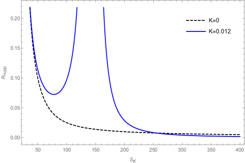
Figure 9: The Ruppeiner scalar versus Kaniadakis entropy plot in the fixed $(J,Q)$ ensemble for $l=1,J=1$ and $Q=2$.

IV.2 Geometrothermodynamic(GTD) formalism

To describe the charged rotaing BTZ black hole in GTD formalism, we first assume a seven-dimensional phase space $\mathcal{T}$ with co-ordinates $M,S,J,Q,T,\Omega$ and $\Phi$ which are the mass, entropy, angular momentum, electric charge, temperature, angular velocity and electric potential for the black hole. The contact 1-form for these set of co-ordinates can be written as:-

$$\Theta=dM-TdS-\Omega dJ-\Phi dQ$$

The 1-form satisfies the condition $\Theta\wedge(d\Theta)^{3}\neq 0$ and a legendre invariant metric that goes by [27]:-

$$G=(dM-TdS-\Omega dJ-\Phi dQ)^{2}+TS(-dTdS+d\Omega dJ+d\Phi dQ)$$

We then assume a three-dimensional sub-space of $\mathcal{T}$ with co-ordinates $E^{a}$ where $a=1,2,3$. We denote this subspace with $\epsilon$ which is defined as a smooth mapping, $\phi:\epsilon\rightarrow\mathcal{T}$. The subspace $\epsilon$ becomes the space of equilibrium states if the pullback of $\phi$ is 0 i.e. $\phi^{*}(\Theta)=0$. A metric structure $g$ is then naturally induced on $\epsilon$ by applying the same pullback on the metric G of $\mathcal{T}$. This induced metric determines all the geometric properties of the equilibrium space for the CR-BTZ black hole.

IV.2.1 The Kaniadakis entropy case

Fixed $(J,Q)$ ensemble:

We write the GTD metric for the Kaniadakis entropy case in the fixed $(J,Q)$ ensemble from the general metric given in (3). We consider the thermodynamic potential $\varphi$ to be the mass $M_{K}$ for the Kaniadakis entropy case in the fixed $(J,Q)$ ensemble as obtained in equation (11). The GTD metric is given by :-

$$g=S_{K}\left(\frac{\partial M_{K}}{\partial S_{K}}\right)\left(-\frac{\partial^{2}M_{K}}{\partial S_{K}^{2}}dS_{K}^{2}+\frac{\partial^{2}M_{K}}{\partial J^{2}}dJ^{2}+\frac{\partial^{2}M_{K}}{\partial Q^{2}}dQ^{2}\right)$$

From the above metric we calculate the GTD scalar for the Kaniadakis entropy case in the fixed $(J,Q)$ ensemble. We have not presented here either the derivation or the final expressions for the GTD scalar due to their considerable length. However obtaining these expressions is fairly straight forward and involves only routine mathematical computations. We present a detailed analysis of the GTD thermodynamic geometry for the Kaniadakis entropy case in the fixed $(J,Q)$ ensemble as follows:

We see from Fig.10 that the GTD scalar $R_{GTD}$ is plotted against the Kaniadakis entropy $S_{K}$ for the Kaniadakis parameter $K=0.012$ in the fixed $(J,Q)$ ensemble. We find that for $l=1,J=1$ and $Q=2$, the GTD scalar has a curvature singularity at $S_{K}=137.69$ for $K=0.012$ as depicted by the blue solid curve whereas for the BH entropy case ($K=0$) the curve remains regular everywhere with no curvature singularities, as is depicted in the figure by the black dashed curve. Unlike Ruppeiner scalar, the singularity obtained from the GTD scalar curve matches exactly with the point of divergence obtained from the corresponding heat capacity curve for the Kaniadakis entropy case in the fixed $(J,Q)$ ensemble.

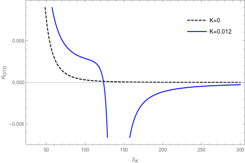
Figure 10: The GTD scalar versus Kaniadakis entropy plot in the fixed $(J,Q)$ ensemble for $l=1,J=1$ and $Q=2$.

Fixed $(\Omega,\Phi)$ ensemble:

We write the GTD metric for the Kaniadakis entropy case in the fixed $(\Omega,\Phi)$ ensemble from the general metric given in (3). We consider the thermodynamic potential $\varphi$ to be the mass $M_{K}$ for the Kaniadakis entropy case in the fixed $(\Omega,\Phi)$ ensemble as obtained in equation (15). The GTD metric is given by :-

$$g=S_{K}\left(\frac{\partial M_{K}}{\partial S_{K}}\right)\left(-\frac{\partial^{2}M_{K}}{\partial S_{K}^{2}}dS_{K}^{2}+\frac{\partial^{2}M_{K}}{\partial\Omega^{2}}d\Omega^{2}+\frac{\partial^{2}M_{K}}{\partial\Phi^{2}}d\Phi^{2}\right)$$

From the above metric we calculate the GTD scalar for the Kaniadakis entropy case in the fixed $(\Omega,\Phi)$ ensemble. We have not shown here either the derivation or the final expressions for the GTD scalar due to their considerable length. However obtaining them is fairly straight forward and involves only routine mathematical computations. We present a detailed analysis of the GTD thermodynamic geometry for the Kaniadakis entropy case in the fixed $(\Omega,\Phi)$ ensemble as follows:

We see from Fig.11 that the GTD scalar $R_{GTD}$ is plotted against the Kaniadakis entropy $S_{K}$ in the fixed $(\Omega,\Phi)$ ensemble. We draw the same plot for $l=1,\Omega=0.2$ and $\Phi=0.1$ for two different entropy ranges in order to make all the appearing curvature singularities visible. We see from Fig.11(a) that the GTD scalar curve has curvature singularities for both the BH $(K=0)$ and Kaniadakis entropy $(K=0.012)$ cases. We find that the curvature singularities are at $S_{K}=11.08(K=0),11.10(K=0.012)$ whereas in Fig.11(b) we find that the GTD scalar has a curvature singularity at $S_{K}=125.74$ for $K=0.012$ with no such behaviour seen for the BH entropy case $(K=0)$. The singularity obtained from the GTD scalar curve matches exactly with the point of divergence obtained from the corresponding heat capacity curve for the Kaniadakis entropy case in the fixed $(\Omega,\Phi)$ ensemble.

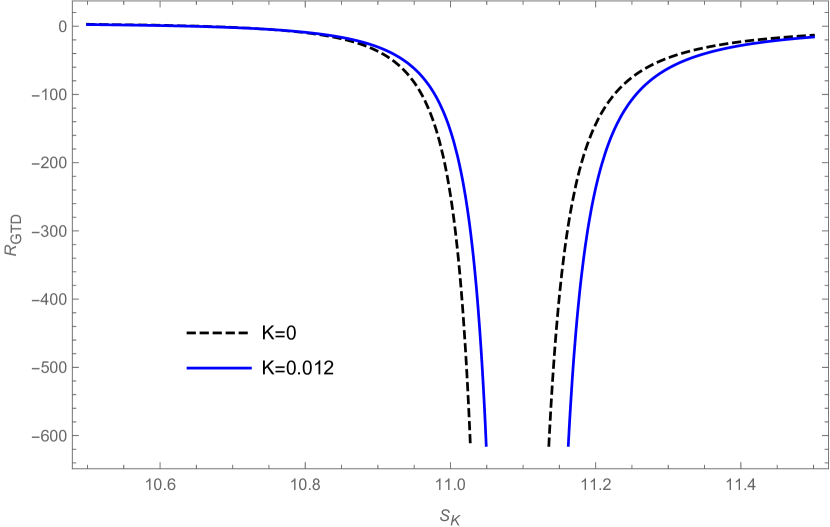
(a) For the range $10<S_{K}<12$

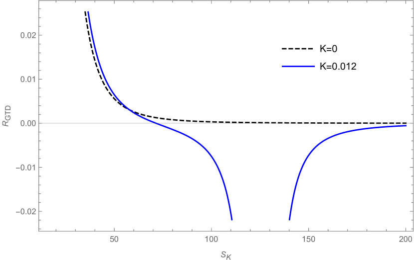
(b) For the range $10<S_{K}<200$

Figure 11: The GTD scalar versus Kaniadakis entropy plot in the fixed $(\Omega,\Phi)$ ensemble for $l=1,\Omega=0.2$ and $\Phi=0.1$.

Fixed $(J,\Phi)$ ensemble:

We write the GTD metric for the Kaniadakis entropy case in the fixed $(J,\Phi)$ ensemble from the general metric given in (3). We consider the thermodynamic potential $\varphi$ to be the mass $M_{K}$ for the Kaniadakis entropy case in the fixed $(J,\Phi)$ ensemble as obtained in equation (18). The GTD metric is given by :-

$$g=S_{K}\left(\frac{\partial M_{K}}{\partial S_{K}}\right)\left(-\frac{\partial^{2}M_{K}}{\partial S_{K}^{2}}dS_{K}^{2}+\frac{\partial^{2}M_{K}}{\partial J^{2}}dJ^{2}+\frac{\partial^{2}M_{K}}{\partial\Phi^{2}}d\Phi^{2}\right)$$

From the above metric we calculate the GTD scalar for the Kaniadakis entropy case in the fixed $(J,\Phi)$ ensemble. We have not shown here either the derivation or the final expressions for the GTD scalar due to their considerable length. However obtaining them is fairly straight forward and involves only routine mathematical computations. We present a detailed analysis of the GTD thermodynamic geometry for the Kaniadakis entropy case in the fixed $(J,\Phi)$ ensemble as follows:

We see from Fig.12 that the GTD scalar $R_{GTD}$ is plotted against the Kaniadakis entropy $S_{K}$ in the fixed $(J,\Phi)$ ensemble. We draw the same plot for $l=1,J=1$ and $\Phi=0.1$ for two different entropy ranges in order to make all the appearing curvature singularities visible. We see from Fig.12(a) that the GTD scalar curve has curvature singularities for both the BH $(K=0)$ and Kaniadakis entropy $(K=0.012)$ cases. We find that the curvature singularities are at $S_{K}=11.42(K=0),11.45(K=0.012)$ whereas in Fig.12(b) we find that the GTD scalar has a curvature singularity at $S_{K}=125.77$ for $K=0.012$ with no such behaviour seen for the BH entropy case $(K=0)$. The singularity obtained from the GTD scalar curve matches exactly with the point of divergence obtained from the corresponding heat capacity curve for the Kaniadakis entropy case in the fixed $(J,\Phi)$ ensemble.

(a) For the range $11<S_{K}<12$

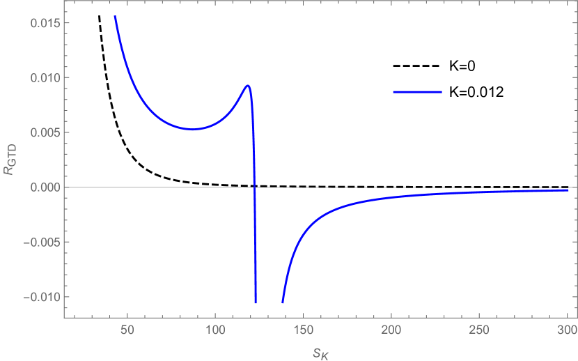
(b) For the range $10<S_{K}<300$

Figure 12: The GTD scalar versus Kaniadakis entropy plot in the fixed $(J,\Phi)$ ensemble for $l=1,J=1$ and $\Phi=0.1$.

Fixed $(\Omega,Q)$ ensemble:

We write the GTD metric for the Kaniadakis entropy case in the fixed $(\Omega,Q)$ ensemble from the general metric given in (3). We consider the thermodynamic potential $\varphi$ to be the mass $M_{K}$ for the Kaniadakis entropy case in the fixed $(J,Q)$ ensemble as obtained in equation (21). The GTD metric is given by :-

$$g=S_{K}\left(\frac{\partial M_{K}}{\partial S_{K}}\right)\left(-\frac{\partial^{2}M_{K}}{\partial S_{K}^{2}}dS_{K}^{2}+\frac{\partial^{2}M_{K}}{\partial\Omega^{2}}d\Omega^{2}+\frac{\partial^{2}M_{K}}{\partial Q^{2}}dQ^{2}\right)$$

From the above metric we calculate the GTD scalar for the Kaniadakis entropy case in the fixed $(\Omega,Q)$ ensemble. We have not presented here either the derivation or the final expressions for the GTD scalar due to their considerable length. However obtaining these expressions is fairly straight forward and involves only routine mathematical computations. We present a detailed analysis of the GTD thermodynamic geometry for the Kaniadakis entropy case in the fixed $(\Omega,Q)$ ensemble as follows:

We see from Fig.13 that the GTD scalar $R_{GTD}$ is plotted against the Kaniadakis entropy $S_{K}$ for the Kaniadakis parameter $K=0.012$ in the fixed $(\Omega,Q)$ ensemble. We find that for $l=1,\Omega=0.2$ and $Q=2$, the GTD scalar has a curvature singularity at $S_{K}=138.16$ for $K=0.012$ as depicted by the blue solid curve whereas for the BH entropy case ($K=0$) the curve remains regular everywhere with no curvature singularities, as is depicted in the figure by the black dashed curve. The singularity obtained from the GTD scalar curve matches exactly with the point of divergence obtained from the corresponding heat capacity curve for the Kaniadakis entropy case in the fixed $(\Omega,Q)$ ensemble.

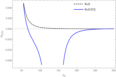
Figure 13: The GTD scalar versus Kaniadakis entropy plot in the fixed $(\Omega,Q)$ ensemble for $l=1,\Omega=0.2$ and $Q=2$

IV.2.2 The Renyi entropy case

We investigate the GTD thermodynamic geometry of the charged rotating BTZ black hole for the case of Renyi entropy. We investigate the GTD scalar for all the four thermodynamic ensembles namely: the fixed $(J,Q)$ ensemble, fixed $(\Omega,\Phi)$ ensemble, fixed $(J,\Phi)$ ensemble and the fixed $(\Omega,Q)$ ensemble. We have not presented here either the derivation or the final expressions for the GTD scalar due to their considerable length. However obtaining these expressions is fairly straight forward and involves only routine mathematical computations.

After investigating all the thermodynamic ensembles, we find that there are curvature singularities in the GTD scalar curves only for the fixed $(\Omega,\Phi)$ and the fixed $(J,\Phi)$ ensembles. The other two thermodynamic ensembles were found to show no such behaviour. We therefore present a detailed analysis of the GTD geometry for the Renyi entropy case in the fixed $(\Omega,\Phi)$ and the fixed $(J,\Phi)$ ensembles as follows:

Fixed $(\Omega,\Phi)$ ensemble:

We write the GTD metric for the Renyi entropy case in the fixed $(\Omega,\Phi)$ ensemble from the general metric given in (3). We consider the thermodynamic potential $\varphi$ to be the mass $M_{R}$ for the Renyi entropy case in the fixed $(\Omega,\Phi)$ ensemble as obtained in equation (25). The GTD metric is given by :-

$$g=S_{R}\left(\frac{\partial M_{R}}{\partial S_{R}}\right)\left(-\frac{\partial^{2}M_{R}}{\partial S_{R}^{2}}dS_{R}^{2}+\frac{\partial^{2}M_{R}}{\partial\Omega^{2}}d\Omega^{2}+\frac{\partial^{2}M_{R}}{\partial\Phi^{2}}d\Phi^{2}\right)$$

We see from Fig.14(a) that the GTD scalar, $R_{GTD}$ for the charged rotating BTZ black hole is plotted against the Renyi entropy, $S_{R}$ in the fixed $(\Omega,\Phi)$ ensemble. We see that for $l=1,\Omega=0.2$ and $\Phi=0.1$ there are curvature singularities in the GTD scalar curve for both the Renyi $(\lambda=0.012)$ and Bekenstein-Hawking (BH) entropy $(\lambda=0)$ cases. We find that for $\lambda=0.012$ there is a curvature singularity observed in the GTD scalar curve at $S_{R}=10.44$ as depicted by the solid green curve in the figure. For the BH entropy case ($\lambda=0$) we find that the GTD scalar has a curvature singularity at $S_{R}=11.08$ as shown in the figure by the black dashed curve. These singularities match exactly with the points of Davies type phase transitions observed in the corresponding heat capacity curve in the fixed $(\Omega,\Phi)$ ensemble. There are two additional curvature singularities observed in the figure for both the Renyi and BH entropy cases, however it was found that these additional curvature singularities correspond to the points where the heat capacity goes to zero for both the Renyi and BH entropy cases in the fixed $(\Omega,\Phi)$ ensemble.

Fixed $(J,\Phi)$ ensemble:

We write the GTD metric for the Renyi entropy case in the fixed $(J,\Phi)$ ensemble from the general metric given in (3). We consider the thermodynamic potential $\varphi$ to be the mass $M_{R}$ for the Renyi entropy case in the fixed $(J,\Phi)$ ensemble as obtained in equation (28). The GTD metric is given by :-

$$g=S_{R}\left(\frac{\partial M_{R}}{\partial S_{R}}\right)\left(-\frac{\partial^{2}M_{R}}{\partial S_{R}^{2}}dS_{R}^{2}+\frac{\partial^{2}M_{R}}{\partial J^{2}}dJ^{2}+\frac{\partial^{2}M_{R}}{\partial\Phi^{2}}d\Phi^{2}\right)$$

We see from Fig.14(b) that the GTD scalar, $R_{GTD}$ for the charged rotating BTZ black hole is plotted against the Renyi entropy, $S_{R}$ in the fixed $(J,\Phi)$ ensemble. We see that for $l=1,J=1$ and $\Phi=0.1$ there are curvature singularities in the GTD scalar curve for both the Renyi $(\lambda=0.012)$ and Bekenstein-Hawking (BH) entropy $(\lambda=0)$ cases. We find that for $\lambda=0.012$ there is a curvature singularity observed in the GTD scalar curve at $S_{R}=10.71$ as depicted by the solid green curve in the figure. For the BH entropy case ($\lambda=0$) we find that the GTD scalar has a curvature singularity at $S_{R}=11.42$ as shown in the figure by the black dashed curve. These singularities match exactly with the points of Davies type phase transitions observed in the corresponding heat capacity curve in the fixed $(J,\Phi)$ ensemble. There are two additional curvature singularities observed in the figure for both the Renyi and BH entropy cases, however it was found that these additional curvature singularities correspond to the points where the heat capacity goes to zero for both the Renyi and BH entropy cases in the fixed $(J,\Phi)$ ensemble.

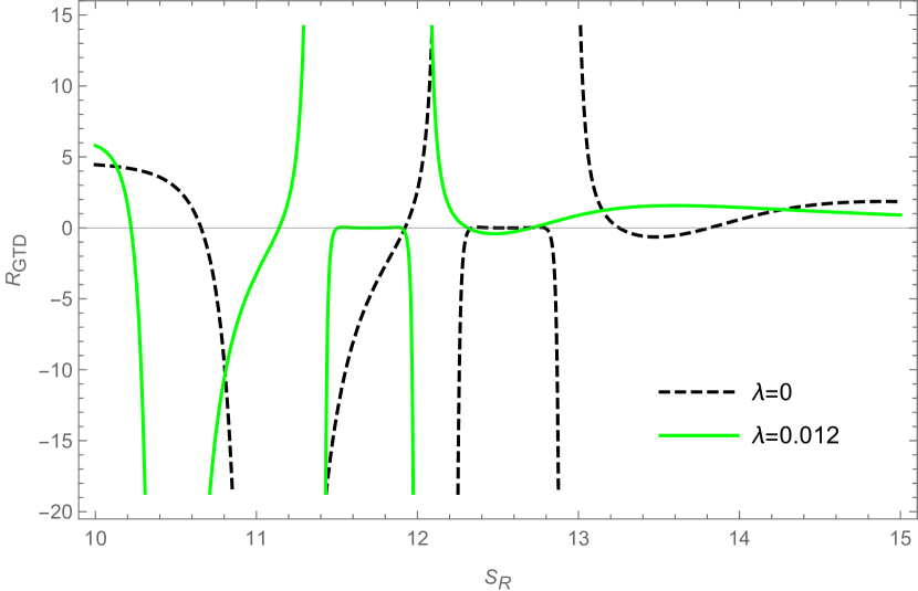
(a) GTD scalar in the fixed $(\Omega,\Phi)$ ensemble for $l=1,\Omega=0.2$ and $\Phi=0.1$.

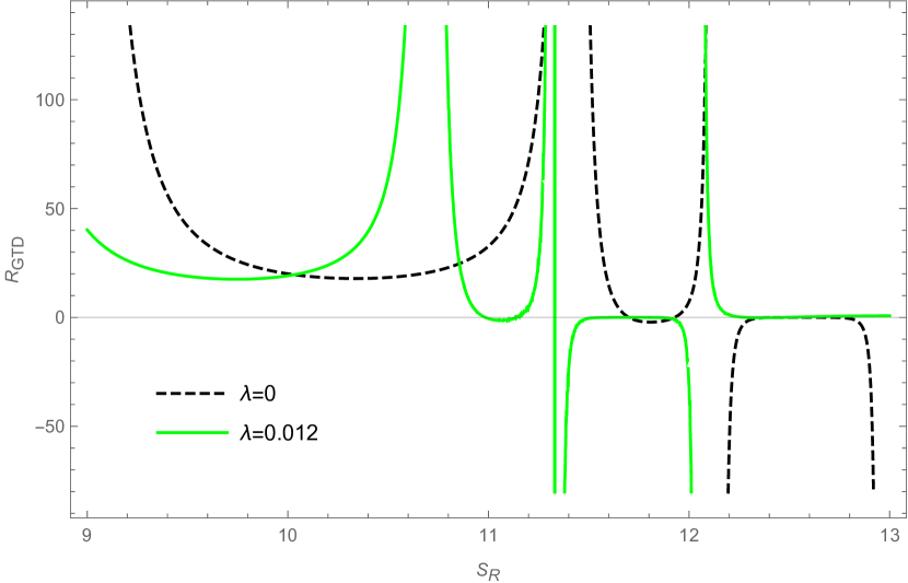
(b) GTD scalar in the fixed $(J,\Phi)$ ensemble for $l=1,J=1$ and $\Phi=0.1$.

Figure 14: The GTD scalar versus Renyi entropy plot for the fixed $(\Omega,\phi)$ and fixed $(J,\Phi)$ ensembles.

IV.2.3 The Sharma-Mittal entropy case

We investigate the GTD thermodynamic geometry of the charged rotating BTZ black hole for the case of Sharma-Mittal entropy. We investigate the GTD scalar for all the four thermodynamic ensembles namely: the fixed $(J,Q)$ ensemble, fixed $(\Omega,\Phi)$ ensemble, fixed $(J,\Phi)$ ensemble and the fixed $(\Omega,Q)$ ensemble. We have not presented here either the derivation or the final expressions for the GTD scalar due to their considerable length. However obtaining these expressions is fairly straight forward and involves only routine mathematical computations.

After investigating all the thermodynamic ensembles, we find that there are curvature singularities in the GTD scalar curves only for the fixed $(\Omega,\Phi)$ and the fixed $(J,\Phi)$ ensembles. The other two thermodynamic ensembles were found to show no such behaviour. We therefore present a detailed analysis of the GTD geometry for the Sharma-Mittal entropy case in the fixed $(\Omega,\Phi)$ and the fixed $(J,\Phi)$ ensembles as follows:

Fixed $(\Omega,\Phi)$ ensemble:

We write the GTD metric for the Sharma-Mittal entropy case in the fixed $(\Omega,\Phi)$ ensemble from the general metric given in (3). We consider the thermodynamic potential $\varphi$ to be the mass $M_{SM}$ for the Sharma-Mittal entropy case in the fixed $(\Omega,\Phi)$ ensemble as obtained in equation (32). The GTD metric is given by :-

$$g=S_{SM}\left(\frac{\partial M_{SM}}{\partial S_{SM}}\right)\left(-\frac{\partial^{2}M_{SM}}{\partial S_{SM}^{2}}dS_{SM}^{2}+\frac{\partial^{2}M_{SM}}{\partial\Omega^{2}}d\Omega^{2}+\frac{\partial^{2}M_{SM}}{\partial\Phi^{2}}d\Phi^{2}\right)$$

We see from Fig.15(a) that the GTD scalar, $R_{GTD}$ for the charged rotating BTZ black hole is plotted against the Sharma-Mittal entropy, $S_{SM}$ in the fixed $(\Omega,\Phi)$ ensemble. We see that for $l=1,\Omega=0.2$ and $\Phi=0.1$ there are curvature singularities in the GTD scalar curve for both the Sharma-Mittal $(\lambda=0.67\rho)$ and Bekenstein-Hawking (BH) entropy $(\lambda=\rho)$ cases. We find that for $\lambda=0.67\rho$ there is a curvature singularity observed in the GTD scalar curve at $S_{SM}=12.32$ as depicted by the solid orange curve in the figure. For the BH entropy case ($\lambda=\rho$) we find that the GTD scalar has a curvature singularity at $S_{SM}=11.08$ as shown in the figure by the black dashed curve. These singularities match exactly with the points of Davies type phase transitions observed in the corresponding heat capacity curve in the fixed $(\Omega,\Phi)$ ensemble. There are two additional curvature singularities observed in the figure for both the Sharma-Mittal and BH entropy cases, however it was found that these additional curvature singularities correspond to the points where the heat capacity goes to zero for both the Sharma-Mittal and BH entropy cases in the fixed $(\Omega,\Phi)$ ensemble.

Fixed $(J,\Phi)$ ensemble:

We write the GTD metric for the Sharma-Mittal entropy case in the fixed $(J,\Phi)$ ensemble from the general metric given in (3). We consider the thermodynamic potential $\varphi$ to be the mass $M_{SM}$ for the Sharma-Mittal entropy case in the fixed $(J,\Phi)$ ensemble as obtained in equation (37). The GTD metric is given by :-

$$g=S_{SM}\left(\frac{\partial M_{SM}}{\partial S_{SM}}\right)\left(-\frac{\partial^{2}M_{SM}}{\partial S_{SM}^{2}}dS_{SM}^{2}+\frac{\partial^{2}M_{SM}}{\partial J^{2}}dJ^{2}+\frac{\partial^{2}M_{SM}}{\partial\Phi^{2}}d\Phi^{2}\right)$$

We see from Fig.15(b) that the GTD scalar, $R_{GTD}$ for the charged rotating BTZ black hole is plotted against the Sharma-Mittal entropy, $S_{SM}$ in the fixed $(J,\Phi)$ ensemble. We see that for $l=1,J=1$ and $\Phi=0.1$ there are curvature singularities in the GTD scalar curve for both the Sharma-Mittal $(\lambda=0.67\rho)$ and Bekenstein-Hawking (BH) entropy $(\lambda=\rho)$ cases. We find that for $\lambda=0.67\rho$ there is a curvature singularity observed in the GTD scalar curve at $S_{SM}=12.84$ as depicted by the solid orange curve in the figure. For the BH entropy case ($\lambda=\rho$) we find that the GTD scalar has a curvature singularity at $S_{SM}=11.42$ as shown in the figure by the black dashed curve. These singularities match exactly with the points of Davies type phase transitions observed in the corresponding heat capacity curve in the fixed $(J,\Phi)$ ensemble. There are two additional curvature singularities observed in the figure for both the Sharma-Mittal and BH entropy cases, however it was found that these additional curvature singularities correspond to the points where the heat capacity goes to zero for both the Sharma-Mittal and BH entropy cases in the fixed $(J,\Phi)$ ensemble.

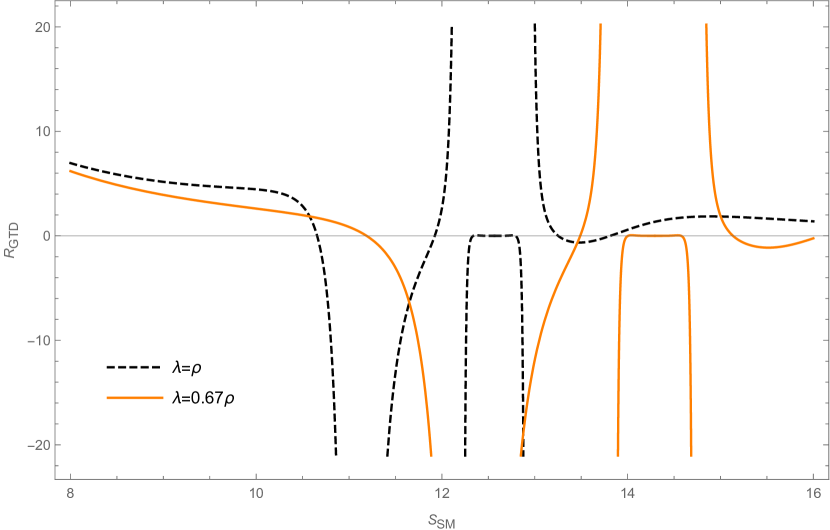
(a) GTD scalar in the fixed $(\Omega,\Phi)$ ensemble for $l=1,\Omega=0.2$ and $\Phi=0.1$.

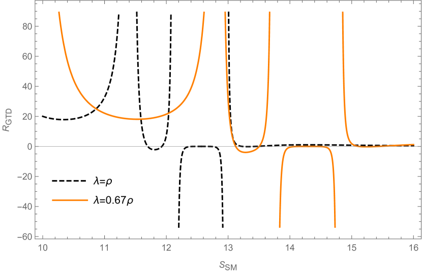
(b) GTD scalar in the fixed $(J,\Phi)$ ensemble for $l=1,J=1$ and $\Phi=0.1$.

Figure 15: The GTD scalar versus Sharma-Mittal entropy plot for the fixed $(\Omega,\phi)$ and fixed $(J,\Phi)$ ensembles.

IV.2.4 The Tsallis-Cirto entropy case

We investigate the GTD thermodynamic geometry of the charged rotating BTZ black hole for the case of Tsallis-Cirto entropy. We investigate the GTD scalar for all the four thermodynamic ensembles namely: the fixed $(J,Q)$ ensemble, fixed $(\Omega,\Phi)$ ensemble, fixed $(J,\Phi)$ ensemble and the fixed $(\Omega,Q)$ ensemble. We have not presented here either the derivation or the final expressions for the GTD scalar due to their considerable length. However obtaining these expressions is fairly straight forward and involves only routine mathematical computations.

After investigating all the thermodynamic ensembles, we find that there are curvature singularities in the GTD scalar curves only for the fixed $(\Omega,\Phi)$ and the fixed $(J,\Phi)$ ensembles. The other two thermodynamic ensembles were found to show no such behaviour. We therefore present a detailed analysis of the GTD geometry for the Tsallis-Cirto entropy case in the fixed $(\Omega,\Phi)$ and the fixed $(J,\Phi)$ ensembles as follows:

Fixed $(\Omega,\Phi)$ ensemble:

We write the GTD metric for the Tsallis-Cirto entropy case in the fixed $(\Omega,\Phi)$ ensemble from the general metric given in (3). We consider the thermodynamic potential $\varphi$ to be the mass $M_{\delta}$ for the Tsallis-Cirto entropy case in the fixed $(\Omega,\Phi)$ ensemble as obtained in equation (41). The GTD metric is given by :-

$$g=S_{\delta}\left(\frac{\partial M_{\delta}}{\partial S_{\delta}}\right)\left(-\frac{\partial^{2}M_{\delta}}{\partial S_{\delta}^{2}}dS_{\delta}^{2}+\frac{\partial^{2}M_{\delta}}{\partial\Omega^{2}}d\Omega^{2}+\frac{\partial^{2}M_{\delta}}{\partial\Phi^{2}}d\Phi^{2}\right)$$

We see from Fig.16(a) that the GTD scalar, $R_{GTD}$ for the charged rotating BTZ black hole is plotted against the Tsallis-Cirto entropy, $S_{\delta}$ in the fixed $(\Omega,\Phi)$ ensemble. We see that for $l=1,\Omega=0.2$ and $\Phi=0.1$ there are curvature singularities in the GTD scalar curve for both the Tsallis-Cirto $(\delta=1.12)$ and Bekenstein-Hawking (BH) entropy $(\delta=1)$ cases. We find that for $\delta=1.12$ there is a curvature singularity observed in the GTD scalar curve at $S_{\delta}=14.69$ as depicted by the solid purple curve in the figure. For the BH entropy case ($\delta=1$) we find that the GTD scalar has a curvature singularity at $S_{\delta}=11.08$ as shown in the figure by the black dashed curve. These singularities match exactly with the points of Davies type phase transitions observed in the corresponding heat capacity curve in the fixed $(\Omega,\Phi)$ ensemble. There are two additional curvature singularities observed in the figure for both the Tsallis-Cirto and BH entropy cases, however it was found that these additional curvature singularities correspond to the points where the heat capacity goes to zero for both the Tsallis-Cirto and BH entropy cases in the fixed $(\Omega,\Phi)$ ensemble.

Fixed $(J,\Phi)$ ensemble:

We write the GTD metric for the Tsallis-Cirto entropy case in the fixed $(J,\Phi)$ ensemble from the general metric given in (3). We consider the thermodynamic potential $\varphi$ to be the mass $M_{\delta}$ for the Tsallis-Cirto entropy case in the fixed $(J,\Phi)$ ensemble as obtained in equation (43). The GTD metric is given by :-

$$g=S_{\delta}\left(\frac{\partial M_{\delta}}{\partial S_{\delta}}\right)\left(-\frac{\partial^{2}M_{\delta}}{\partial S_{\delta}^{2}}dS_{\delta}^{2}+\frac{\partial^{2}M_{\delta}}{\partial J^{2}}dJ^{2}+\frac{\partial^{2}M_{\delta}}{\partial\Phi^{2}}d\Phi^{2}\right)$$

We see from Fig.16(b) that the GTD scalar, $R_{GTD}$ for the charged rotating BTZ black hole is plotted against the Tsallis-Cirto entropy, $S_{\delta}$ in the fixed $(J,\Phi)$ ensemble. We see that for $l=1,J=1$ and $\Phi=0.1$ there are curvature singularities in the GTD scalar curve for both the the Tsallis-Cirto $(\delta=1.12)$ and Bekenstein-Hawking (BH) entropy $(\delta=1)$ cases. We find that for $\delta=1.12$ there is a curvature singularity observed in the GTD scalar curve at $S_{\delta}=15.28$ as depicted by the solid purple curve in the figure. For the BH entropy case ($\delta=1$) we find that the GTD scalar has a curvature singularity at $S_{\delta}=11.42$ as shown in the figure by the black dashed curve. These singularities match exactly with the points of Davies type phase transitions observed in the corresponding heat capacity curve in the fixed $(J,\Phi)$ ensemble. There are two additional curvature singularities observed in the figure for both the Tsallis-Cirto and BH entropy cases, however it was found that these additional curvature singularities correspond to the points where the heat capacity goes to zero for both the Tsallis-Cirto and BH entropy cases in the fixed $(J,\Phi)$ ensemble.

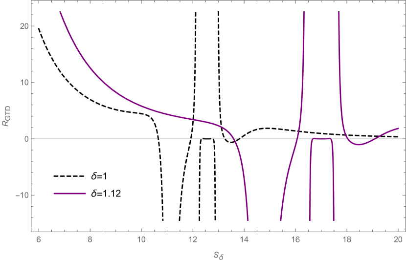
(a) GTD scalar in the fixed $(\Omega,\Phi)$ ensemble for $l=1,\Omega=0.2$ and $\Phi=0.1$.

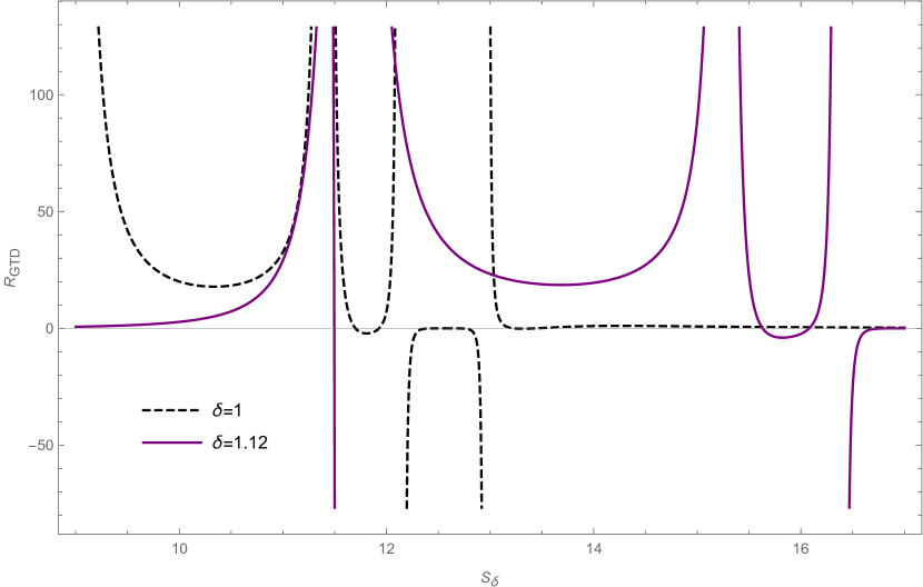
(b) GTD scalar in the fixed $(J,\Phi)$ ensemble for $l=1,J=1$ and $\Phi=0.1$.

Figure 16: The GTD scalar versus Tsallis-Cirto entropy plot for the fixed $(\Omega,\phi)$ and fixed $(J,\Phi)$ ensembles.

IV.2.5 The Barrow entropy case

We investigate the GTD thermodynamic geometry of the charged rotating BTZ black hole for the case of Barrow entropy. We investigate the GTD scalar for all the four thermodynamic ensembles namely: the fixed $(J,Q)$ ensemble, fixed $(\Omega,\Phi)$ ensemble, fixed $(J,\Phi)$ ensemble and the fixed $(\Omega,Q)$ ensemble. We have not presented here either the derivation or the final expressions for the GTD scalar due to their considerable length. However obtaining these expressions is fairly straight forward and involves only routine mathematical computations.

After investigating all the thermodynamic ensembles, we find that there are curvature singularities in the GTD scalar curves only for the fixed $(\Omega,\Phi)$ and the fixed $(J,\Phi)$ ensembles. The other two thermodynamic ensembles were found to show no such behaviour. We therefore present a detailed analysis of the GTD geometry for the Barrow entropy case in the fixed $(\Omega,\Phi)$ and the fixed $(J,\Phi)$ ensembles as follows:

Fixed $(\Omega,\Phi)$ ensemble:

We write the GTD metric for the Barrow entropy case in the fixed $(\Omega,\Phi)$ ensemble from the general metric given in (3). We consider the thermodynamic potential $\varphi$ to be the mass $M_{\Delta}$ for the Barrow entropy case in the fixed $(\Omega,\Phi)$ ensemble as obtained in equation (45). The GTD metric is given by :-

$$g=S_{\Delta}\left(\frac{\partial M_{\Delta}}{\partial S_{\Delta}}\right)\left(-\frac{\partial^{2}M_{\Delta}}{\partial S_{\Delta}^{2}}dS_{\Delta}^{2}+\frac{\partial^{2}M_{\Delta}}{\partial\Omega^{2}}d\Omega^{2}+\frac{\partial^{2}M_{\Delta}}{\partial\Phi^{2}}d\Phi^{2}\right)$$

We see from Fig.17(a) that the GTD scalar, $R_{GTD}$ for the charged rotating BTZ black hole is plotted against the Barrow entropy, $S_{\Delta}$ in the fixed $(\Omega,\Phi)$ ensemble. We see that for $l=1,\Omega=0.2$ and $\Phi=0.1$ there are curvature singularities in the GTD scalar curve for both the Barrow $(\Delta=0.12)$ and Bekenstein-Hawking (BH) entropy $(\Delta=0)$ cases. We find that for $\Delta=0.12$ there is a curvature singularity observed in the GTD scalar curve at $S_{\Delta}=12.76$ as depicted by the solid red curve in the figure. For the BH entropy case ($\Delta=0$) we find that the GTD scalar has a curvature singularity at $S_{\Delta}=11.08$ as shown in the figure by the black dashed curve. These singularities match exactly with the points of Davies type phase transitions observed in the corresponding heat capacity curve in the fixed $(\Omega,\Phi)$ ensemble. There are two additional curvature singularities observed in the figure for both the Barrow and BH entropy cases, however it was found that these additional curvature singularities correspond to the points where the heat capacity goes to zero for both the Barrow and BH entropy cases in the fixed $(\Omega,\Phi)$ ensemble.

Fixed $(J,\Phi)$ ensemble:

We write the GTD metric for the Barrow entropy case in the fixed $(J,\Phi)$ ensemble from the general metric given in (3). We consider the thermodynamic potential $\varphi$ to be the mass $M_{\delta}$ for the Barrow entropy case in the fixed $(J,\Phi)$ ensemble as obtained in equation (46). The GTD metric is given by :-

$$g=S_{\Delta}\left(\frac{\partial M_{\Delta}}{\partial S_{\Delta}}\right)\left(-\frac{\partial^{2}M_{\Delta}}{\partial S_{\Delta}^{2}}dS_{\Delta}^{2}+\frac{\partial^{2}M_{\Delta}}{\partial J^{2}}dJ^{2}+\frac{\partial^{2}M_{\Delta}}{\partial\Phi^{2}}d\Phi^{2}\right)$$

We see from Fig.17(b) that the GTD scalar, $R_{GTD}$ for the charged rotating BTZ black hole is plotted against the Barrow entropy, $S_{\Delta}$ in the fixed $(J,\Phi)$ ensemble. We see that for $l=1,J=1$ and $\Phi=0.1$ there are curvature singularities in the GTD scalar curve for both the Barrow $(\Delta=0.12)$ and Bekenstein-Hawking (BH) entropy $(\Delta=0)$ cases. We find that for $\Delta=0.12$ there is a curvature singularity observed in the GTD scalar curve at $S_{\Delta}=13.21$ as depicted by the solid red curve in the figure. For the BH entropy case ($\Delta=0$) we find that the GTD scalar has a curvature singularity at $S_{\Delta}=11.42$ as shown in the figure by the black dashed curve. These singularities match exactly with the points of Davies type phase transitions observed in the corresponding heat capacity curve in the fixed $(J,\Phi)$ ensemble. There are two additional curvature singularities observed in the figure for both the Barrow and BH entropy cases, however it was found that these additional curvature singularities correspond to the points where the heat capacity goes to zero for both the Barrow and BH entropy cases in the fixed $(J,\Phi)$ ensemble.

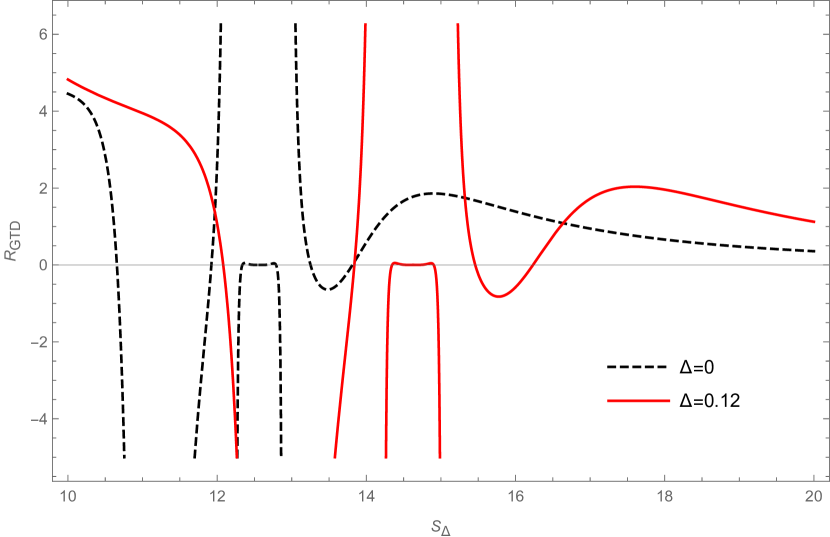
(a) GTD scalar in the fixed $(\Omega,\Phi)$ ensemble for $l=1,\Omega=0.2$ and $\Phi=0.1$.

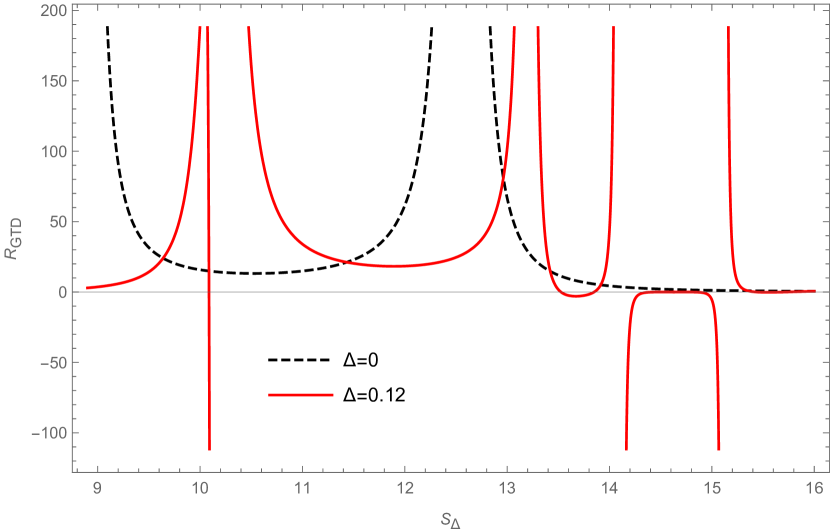
(b) GTD scalar in the fixed $(J,\Phi)$ ensemble for $l=1,J=1$ and $\Phi=0.1$.

Figure 17: The GTD scalar versus Barrow entropy plot for the fixed $(\Omega,\phi)$ and fixed $(J,\Phi)$ ensembles.

V Conclusions:

We have investigated the thermodynamics and the thermodynamic geometry of CR-BTZ black hole in four different ensembles namely: the fixed $(J,Q)$ ensemble, fixed $(\Omega,\Phi)$ ensemble, fixed $(J,\Phi)$ ensemble and the fixed $(\Omega,Q)$ ensemble considering Kaniadakis entropy, Renyi entropy, Sharma-Mittal entropy, Tsallis-Cirto and Barrow entropy in place of the Bekenstein-Hawking entropy. In Kaniadakis entropy case, a Davies type phase transition was observed in all the ensembles. Contrary to this, no such behaviour was observed in the Bekenstein-Hawking entropy case[27]. Both the Ruppeiner and the GTD scalar were observed to have curvature singularities corresponding to Davies type of phase transitions in the corresponding cases. The location of the curvature singularities in the GTD scalar exactly matched the Davies type phase transition points in all the ensembles. The Ruppeiner scalar, although showed curvature singularities, the location of those singularities were found to be not exactly the same as the corresponding Davies type transition points. For all the other non-extensive entropy cases, the thermodynamic structure were found to resemble their counterparts in the Bekenstein-Hawking entropy. A table summarising our results is presented below where we write the number of Davies type phase transition points observed against each of the non extensive entropy cases along with the BH entropy for all the four thermodynamic ensembles:

	Entropy	Fixed $(J,Q)$ ensemble	Fixed $(\Omega,\Phi)$ ensemble	Fixed $(J,\Phi)$ ensemble	Fixed $(\Omega,Q)$ ensemble
	Bekenstein-Hawking	0	1	1	0
	Kaniadakis	1	2	2	1
	Renyi	0	1	1	0
	Sharma-Mittal	0	1	1	0
	Tsallis-Cirto	0	1	1	0
	Barrow	0	1	1	0

To conclude, our analysis shows that the thermodynamic phase structure on $(2+1)$ dimensional CR-BTZ black hole with Kaniadakis entropy differs from the one with the conventional Bekenstein-Hawking entropy in all the ensembles. This result is in contrast to that found in [16], in the context of charged AdS black holes where both Kaniadakis entropy and Bekenstein-Hawking entropy yielded similar phase structures. It will be interesting to extend the study of black hole thermodynamics in the framework of non-extensive entropy to other black holes to get a clearer picture. We plan to address this issue in our future works.

VI Acknowledgments

The authors would like to thank Himanshu Bora for numerous enlightening discussions and certain exquisite suggestions he offered during the course of this work.

References

- Hawking [1975] S. W. Hawking, Particle creation by black holes, Communications in mathematical physics 43, 199 (1975).
- Bekenstein [1973] J. D. Bekenstein, Black holes and entropy, Physical Review D 7, 2333 (1973).
- Hawking [1976] S. W. Hawking, Black holes and thermodynamics, Physical Review D 13, 191 (1976).
- Cai et al. [2013] R.-G. Cai, L.-M. Cao, L. Li, and R.-Q. Yang, Pv criticality in the extended phase space of gauss-bonnet black holes in ads space, Journal of High Energy Physics 2013, 1 (2013).
- Kubizňák et al. [2017] D. Kubizňák, R. B. Mann, and M. Teo, Black hole chemistry: thermodynamics with lambda, Classical and Quantum Gravity 34, 063001 (2017).
- Visser [2022] M. R. Visser, Holographic thermodynamics requires a chemical potential for color, Physical Review D 105, 106014 (2022).
- Cong et al. [2021] W. Cong, D. Kubizňák, and R. B. Mann, Thermodynamics of ads black holes: critical behavior of the central charge, Physical Review Letters 127, 091301 (2021).
- Gao and Zhao [2022] Z. Gao and L. Zhao, Restricted phase space thermodynamics for ads black holes via holography, Classical and Quantum Gravity 39, 075019 (2022).
- Gao et al. [2022] Z. Gao, X. Kong, and L. Zhao, Thermodynamics of kerr-ads black holes in the restricted phase space, The European Physical Journal C 82, 112 (2022).
- Kaniadakis [2002] G. Kaniadakis, Statistical mechanics in the context of special relativity, Physical review E 66, 056125 (2002).
- Drepanou et al. [2022] N. Drepanou, A. Lymperis, E. N. Saridakis, and K. Yesmakhanova, Kaniadakis holographic dark energy and cosmology, The European Physical Journal C 82, 449 (2022).
- Rényi [1959] A. Rényi, On the dimension and entropy of probability distributions, Acta Mathematica Academiae Scientiarum Hungarica 10, 193 (1959).
- Masi [2005] M. Masi, A step beyond tsallis and rényi entropies, Physics Letters A 338, 217 (2005).
- Tsallis and Cirto [2013] C. Tsallis and L. J. Cirto, Black hole thermodynamical entropy, The European Physical Journal C 73, 1 (2013).
- Barrow [2020] J. D. Barrow, The area of a rough black hole, Physics Letters B 808, 135643 (2020).
- Luciano and Saridakis [2023] G. G. Luciano and E. Saridakis, P- v criticalities, phase transitions and geometrothermodynamics of charged ads black holes from kaniadakis statistics, Journal of High Energy Physics 2023, 1 (2023).
- Promsiri et al. [2022] C. Promsiri, E. Hirunsirisawat, and R. Nakarachinda, Emergent phase, thermodynamic geometry, and criticality of charged black holes from rényi statistics, Physical Review D 105, 124049 (2022).
- Ghaffari et al. [2019] S. Ghaffari, A. Ziaie, H. Moradpour, F. Asghariyan, F. Feleppa, and M. Tavayef, Black hole thermodynamics in sharma–mittal generalized entropy formalism, General Relativity and Gravitation 51, 1 (2019).
- Luciano and Sheykhi [2023] G. G. Luciano and A. Sheykhi, Black hole geometrothermodynamics and critical phenomena: A look from tsallis entropy-based perspective, Physics of the Dark Universe 42, 101319 (2023).
- Jawad and Fatima [2022] A. Jawad and S. R. Fatima, Thermodynamic geometries analysis of charged black holes with barrow entropy, Nuclear Physics B 976, 115697 (2022).
- Saridakis [2020] E. N. Saridakis, Barrow holographic dark energy, Physical Review D 102, 123525 (2020).
- Saridakis et al. [2018] E. N. Saridakis, K. Bamba, R. Myrzakulov, and F. K. Anagnostopoulos, Holographic dark energy through tsallis entropy, Journal of Cosmology and Astroparticle Physics 2018 (12), 012.
- Tavayef et al. [2018] M. Tavayef, A. Sheykhi, K. Bamba, and H. Moradpour, Tsallis holographic dark energy, Physics Letters B 781, 195 (2018).
- Shababi and Ourabah [2020] H. Shababi and K. Ourabah, Non-gaussian statistics from the generalized uncertainty principle, The European Physical Journal Plus 135, 697 (2020).
- Luciano [2021] G. G. Luciano, Tsallis statistics and generalized uncertainty principle, The European Physical Journal C 81, 672 (2021).
- Moussa [2021] M. Moussa, Schwarzschild black hole thermodynamics and generalized uncertainty principle, International Journal of Theoretical Physics 60, 994 (2021).
- Akbar et al. [2011] M. Akbar, H. Quevedo, K. Saifullah, A. Sanchez, and S. Taj, Thermodynamic geometry of charged rotating btz black holes, Physical Review D—Particles, Fields, Gravitation, and Cosmology 83, 084031 (2011).
- Wang et al. [2020] P. Wang, H. Wu, and H. Yang, Thermodynamic geometry of ads black holes and black holes in a cavity, The European Physical Journal C 80, 1 (2020).
- Shahzad et al. [2022] M. U. Shahzad, M. I. Asjad, and S. Nafees, Study of thermodynamical geometries of conformal gravity black hole, The European Physical Journal C 82, 1044 (2022).
- Wu et al. [2021] B. Wu, C. Wang, Z.-M. Xu, and W.-L. Yang, Ruppeiner geometry and thermodynamic phase transition of the black hole in massive gravity, The European Physical Journal C 81, 1 (2021).
- Weinhold [1975] F. Weinhold, Metric geometry of equilibrium thermodynamics, The Journal of Chemical Physics 63, 2479 (1975).
- Ruppeiner [1979] G. Ruppeiner, Thermodynamics: A riemannian geometric model, Physical Review A 20, 1608 (1979).
- Salamon et al. [1984] P. Salamon, J. Nulton, and E. Ihrig, On the relation between entropy and energy versions of thermodynamic length, The Journal of chemical physics 80, 436 (1984).
- Ruppeiner [1995] G. Ruppeiner, Riemannian geometry in thermodynamic fluctuation theory, Reviews of Modern Physics 67, 605 (1995).
- Mrugała [1984] R. Mrugała, On equivalence of two metrics in classical thermodynamics, Physica A: Statistical Mechanics and its Applications 125, 631 (1984).
- Åman et al. [2003] J. E. Åman, I. Bengtsson, and N. Pidokrajt, Geometry of black hole thermodynamics, General Relativity and Gravitation 35, 1733 (2003).
- Quevedo [2007] H. Quevedo, Geometrothermodynamics, Journal of Mathematical Physics 48 (2007).
- Quevedo [2008] H. Quevedo, Geometrothermodynamics of black holes, General Relativity and Gravitation 40, 971 (2008).
- Soroushfar et al. [2016] S. Soroushfar, R. Saffari, and N. Kamvar, Thermodynamic geometry of black holes in f (r) gravity, The European Physical Journal C 76, 1 (2016).
- Huang and Tao [2022] Y. Huang and J. Tao, Thermodynamics and phase transition of btz black hole in a cavity, Nuclear Physics B 982, 115881 (2022).
- Kaniadakis et al. [1996] G. Kaniadakis, A. Lavagno, and P. Quarati, Generalized fractional statistics, Modern Physics Letters B 10, 497 (1996).
- Kaniadakis et al. [2004] G. Kaniadakis, M. Lissia, and A. Scarfone, Deformed logarithms and entropies, Physica A: Statistical Mechanics and its Applications 340, 41 (2004).
- Kaniadakis [2005] G. Kaniadakis, Statistical mechanics in the context of special relativity. ii., Physical Review E—Statistical, Nonlinear, and Soft Matter Physics 72, 036108 (2005).
- Housset et al. [2024] J. Housset, J. F. Saavedra, and F. Tello-Ortiz, Cosmological flrw phase transitions and micro-structure under kaniadakis statistics, Physics Letters B 853, 138686 (2024).
- Nakarachinda et al. [2022] R. Nakarachinda, C. Promsiri, L. Tannukij, and P. Wongjun, Thermodynamics of black holes with r’enyi entropy from classical gravity, arXiv preprint arXiv:2211.05989 (2022).
- Lenzi et al. [2000] E. Lenzi, R. Mendes, and L. Da Silva, Statistical mechanics based on renyi entropy, Physica A: Statistical Mechanics and its Applications 280 (2000).
- Jizba and Arimitsu [2004a] P. Jizba and T. Arimitsu, The world according to rényi: thermodynamics of multifractal systems, Annals of Physics 312, 17 (2004a).
- Jizba and Arimitsu [2004b] P. Jizba and T. Arimitsu, Observability of rényi’s entropy, Physical review E 69, 026128 (2004b).
- Dowker [2013] J. Dowker, Sphere rényi entropies, Journal of Physics A: Mathematical and Theoretical 46, 225401 (2013).
- Liu and Mezei [2013] H. Liu and M. Mezei, A refinement of entanglement entropy and the number of degrees of freedom, Journal of High Energy Physics 2013, 1 (2013).
- Fursaev [2012] D. V. Fursaev, Entanglement rényi entropies in conformal field theories and holography, Journal of High Energy Physics 2012, 1 (2012).
- Sadeghi et al. [2019] J. Sadeghi, M. Rostami, and M. Alipour, Investigation of phase transition of btz black hole with sharma–mittal entropy approaches, International Journal of Modern Physics A 34, 1950182 (2019).
- Kolesnichenko and Marov [2022] A. Kolesnichenko and M. Y. Marov, Friedmann cosmological equations in the sharma–mittal entropy formalism, Astronomy Reports 66, 786 (2022).
- Naeem and Bibi [2024] M. Naeem and A. Bibi, Correction to the friedmann equation with sharma–mittal entropy: A new perspective on cosmology, Annals of Physics 462, 169618 (2024).
- Chen [2022] G.-R. Chen, Emergence of cosmic space and horizon entropy maximization from tsallis and cirto entropy, The European Physical Journal C 82, 1 (2022).
- Rani et al. [2023] S. Rani, A. Jawad, and M. Hussain, Impact of barrow entropy on geometrothermodynamics of specific black holes, The European Physical Journal C 83, 710 (2023).
- Barrow [1982] J. D. Barrow, Chaotic behaviour in general relativity, Physics Reports 85, 1 (1982).
- Banados et al. [1993] M. Banados, M. Henneaux, C. Teitelboim, and J. Zanelli, Geometry of the 2+ 1 black hole, Physical Review D 48, 1506 (1993).
- Clement [1993] G. Clement, Classical solutions in three-dimensional einstein-maxwell cosmological gravity, Classical and Quantum Gravity 10, L49 (1993).
- Clement [1996] G. Clement, Spinning charged btz black holes and self-dual particle-like solutions, Physics Letters B 367, 70 (1996).
- Martinez et al. [2000] C. Martinez, C. Teitelboim, and J. Zanelli, Charged rotating black hole in three spacetime dimensions, Physical Review D 61, 104013 (2000).
- Achucarro and Ortiz [1993] A. Achucarro and M. E. Ortiz, Relating black holes in two and three dimensions, Physical Review D 48, 3600 (1993).