The Giroux Correspondence in dimension 3
Abstract.
In [LV] the authors proved the Giroux Correspondence for tight contact -manifolds via convex Heegaard surfaces. Simultaneously, [HBH] gave an all-dimensions proof of the Giroux Correspondence by generalising convex surface theory to higher dimensions. This paper uses a key result from [HBH] and also [Tia] to complete the -dimensional proof for arbitrary (not necessarily tight) contact 3-manifolds. This presentation features low-dimensional techniques and further clarifies the relationship between contact manifolds and their Heegaard splittings that was introduced in [LV].
1. Introduction
Topology and contact geometry enjoy a remarkable relationship in dimension . Contact structures are defined in the smooth category with differential geometric language, and yet they mirror fundamental topological properties of the underlying -manifold. An open book decomposition is arguably the most striking incarnation of this relationship: up to diffeomorphism, a contact manifold is determined simply by a surface mapping class. For the last twenty years, 3-dimensional contact geometry has been shaped by the equivalence between contact structures and open books first proposed by Giroux in the early 2000s:
Theorem 1.1.
[Giroux Correspondence [Gir02]] Two open book decompositions support isotopic contact structures if and only if they admit a common positive stabilisation.
Because topology and contact geometry are so closely entwined, it’s natural to probe whether topological techniques can be squeezed to produce meaningful contact geometric outputs. In this spirit, in 2023 the authors developed new tools to study -dimensional contact manifolds via their Heegaard decompositions.
We used the enhanced relationship between contact structures and Heegaard splittings to prove the Giroux Correspondence in the case of tight contact -manifolds [LV]. Simultaneously, Breen-Honda-Huang used generalised convex surface theory to prove the Giroux Correspondence for all contact structures and in all dimensions [HBH]. While the work of Breen-Honda-Huang fully covers the -dimensional case, the generality of their techniques lends their proof a different flavour. This paper completes the 3-dimensional story, using an essential result of [HBH] and also [Tia] to bridge the gap to overtwisted manifolds that limited the scope of our previous paper. We believe this work will make the proof more accessible to a low-dimensional audience; in particular, it offers a useful illustration of convex surface techniques in concert with Heegaard splittings.
1.1. Heegaard splittings and open book decompositions
Any open book decomposition of a manifold gives rise to a canonical Heegaard decomposition. Heegaard splittings produced thus are called convex Heegaard splittings, and one may directly recover an open book supporting from any convex Heegaard splitting of . The innovation in [LV] is a procedure called refinement that produces an open book from a more general class of Heegaard splittings of a contact manifold. Although this open book decomposition is not uniquely defined, any two open books produced thus admit a common positive stabilisation – exactly the equivalence appearing in the Giroux Correspondence. It follows that the Giroux Correspondence can be rephrased as a statement about convex Heegaard splittings (Theorem 3.3). Our proof of the Giroux Correspondence for tight contact manifolds relied on showing that many operations one might naturally perform on a Heegaard splitting of a contact manifold in fact preserve the positive stabilisation class of the associated open book.
However, these techniques were insufficient in the case of overtwisted manifolds. In order to assign an open book decomposition to a contact manifold with a Heegaard splitting, our approach required both handlebodies to be tight. When two convex Heegaard surfaces are isotopic, there is a sequence of convex Heegaard surfaces interpolating between them. However, even when both original Heegaard splittings have tight handlebodies, intermediate Heegaard splittings in the sequence may nevertheless have overtwisted handlebodies. The present work bypasses this stumbling block by considering highly stabilised Heegaard splittings where the handlebodies are always tight. We introduce the term “bridging” for a particular method of constructing such a splitting, and we show that different choices made in constructing a bridge splitting preserve the positive stabilisation class of the associated open book. This allows us to prove that any pair of convex Heegaard splittings for a fixed contact manifold correspond to open books that admit a common positive stabilisation.
1.2. A note on notation
The arguments in this paper involve sequences of Heegaard splittings of varying types, each of which is denoted by some sort of “”. We have attempted to define notation locally and maintain these choices consistently, but we briefly outline the system here for reference. Every Heegaard surface is required to be convex; Heegaard splittings subject to no further restrictions are denoted by , where and are the handlebodies, oriented so that . Elements of a pair of Heegaard splittings are distinguished by the addition of a prime: and . Following the notation in [LV], the refinement of is denoted by .
Starting in Section 3.2, we will stabilise Heegaard splittings by attaching certain contact -handles found in the complement of fixed handlebodies. We will call this process bridging, and we denote the bridge of by . When we bridge only a single handlebody of the original splitting, we denote the result by or , as appropriate. Distinct bridged splittings may be distinguished by primes: and .
Acknowledgment
This research was supported in part by the Austrian Science Fund (FWF) P 34318. For open access purposes, the author has applied a CC BY public copyright license to any author-accepted manuscript version arising from this submission. The authors would also like to thank Ko Honda and Matthias Scharitzer for helpful discussions on the topic.
2. Background
We assume the reader is familiar with basic notions in contact geometry, but we use this section to collect some tools and terminology that will be essential for the rest of the paper. Section 2.1 provides a quick review of convex surface theory and introduces weak contactomorphism (Definition 2.1) as an equivalence relation on contact manifolds with convex boundary. Section 2.2 describes the relationship between open book decompositions and convex Heegaard splittings (Definition 2.4) of a contact manifold. Section 2.3 presents the contact handle model for bypass attachment. Finally, Section 2.4 states the key theorem borrowed from [HBH] and [Tia] which classifies distinct bypass decompositions of a product cobordism. Also, Lemma 2.8 gives a new perspective on the familiar operation of bypass rotation.
2.1. Convex surfaces
The reader looking for a more thorough introduction to convex surface theory is referred to [Mas14] or the lecture notes [Etn04, Hon].
Recall that a vector field in a contact manifold is contact if the flow of the vector field preserves . A surface is convex when there exists a contact vector field transverse to . The essential feature of a convex surface is that it provides a combinatorial characterisation of the contact structure in an -invariant neighbourhood ; the product structure on is provided by the flow of . The dividing set on is a separating multicurve consisting of the points where lies in . Changing the vector field that certifies as convex changes only by isotopy, and any isotopy keeping convex also preserves up to isotopy. Furthermore, any isotopic to may be realised as a dividing set after performing an isotopy of within an -invariant neighbourhood.
Convex surface theory is particularly useful for studying contact manifolds with boundary, and we will assume throughout that the boundary of is convex. Since the dividing set characterises near , we would like to be able to glue to whenever there is a diffeomorphism taking to . Because we are working in the smooth category, gluing is achieved by identifying contact neighbourhoods of the boundaries; for later convenience, we introduce the following equivalence relation on contact manifolds with boundary:
Definition 2.1.
[LV, Definition 2.3.] Two contact manifolds and with convex boundary are weakly contactomorphic if there is a contact embedding such that is convexly isotopic to .
Remark 2.2.
We note that if is a contact embeddeding as above, then is a weak identity morphism in the sense of [Tia].
Henceforth, we will be interested in contact manifolds with boundary only up to weak contactomorphism. Two (weak contactomorphism classes of) manifolds may be glued along diffeomorphic boundary components if and only if there is a diffeomorphism respecting the dividing sets. Gluing is well defined as an operation on weak contactomorphism classes of manifolds; see [LV, Proposition 2.8.].
As a special case of weakly contactomorphic manifolds, we also introduce the following:
Definition 2.3.
[LV, Definition 2.4.] Two embedded codimension- submanifolds with convex boundary are weakly (contact) isotopic if there is an isotopy between them such that remains convex throughout.
2.2. Open book decompositions of contact manifolds
Let denote an open book decomposition of . That is, is an oriented link and is a fibration of the complement of by Seifert surfaces for . When is equipped with a contact structure , we assume any open book decomposition supports in the sense of [TW75].
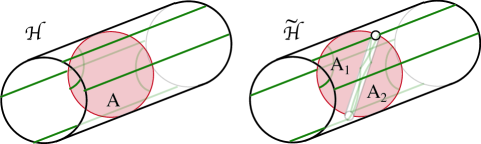
An open book decomposition induces a Heegaard splitting where each handlebody consists of half the pages: and . The Heegaard surface
is naturally convex with dividing curve . An arc properly embedded on a page of the open book produces a properly embedded disc in the corresponding handlebody, and in fact, such discs characterise the Heegaard splittings induced by open books.
More precisely, a disc properly embedded in a contact manifold with convex boundary is a product disc if . A disc system for a handlebody is a set of properly embedded discs that cut it into a ball. Torisu introduced the notion of a convex Heegaard splitting [Tor00]:
Definition 2.4.
A Heegaard splitting of is convex if
-
•
is convex with dividing curve ;
-
•
and are both tight; and
-
•
each of the manifolds and admits a system of product discs.
The discs in a convex Heegaard splitting determine a product structure on each handlebody, and hence, an open book decomposition with binding . Moreover, this relation is one-to-one up to isotopy.
Proposition 2.5.
[LV, Proposition 3.4.] Let be a contact manifold and let and be open books supporting . Then the induced convex Heegaard splittings are isotopic via an isotopy keeping the Heegaard surface convex if and only if and are isotopic through a path of open books supporting .
Because a convex Heegaard splitting determines an open book decomposition, a convex splitting allows one to reconstruct the contact structure. Specifically, suppose is a convex Heegaard diagram for where the meridional circles bound product discs in the respective handlebodies and the restriction of to each handlebody is known to be tight. Then up to contact isotopy, there is a unique contact structure structure compatible with this data.
2.3. Bypass attachment
Next, we turn to an operation that changes the weak contactomorphism class of a contact manifold while preserving the topological type. Adopting the perspective of [HKM09, Ozb11], we define bypass attachment as an operation performed by gluing contact handles.
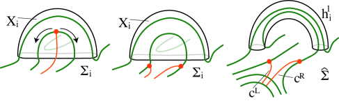
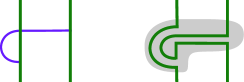
As in the topological setting, a contact -handle is a glued along to the boundary of an existing manifold . Additionally, each -handle is required to smooth to a tight -ball, and the dividing set on the attaching region is prescribed. A -handle attachment is specified by an on the dividing set , while a -handle attachment is specified by an that intersects twice transversely. Local models for handle attachment are well established in the literature; see, for example, [Gir91] or [Ozb11]. Although each handle is a cornered manifold, the gluing process is defined so that the manifold is smooth after each attachment.
Let be a convex surface. A Legendrian arc embedded in is a bypass arc if lies on and the interior of intersects once transversely. As explained next, we may associate a new contact manifold with convex boundary to any bypass arc on the convex boundary of a contact manifold.
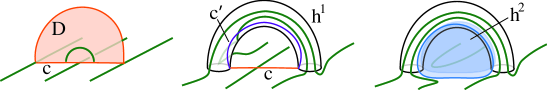
The steps described here are illustrated in Figure 1. First, attach a minimally twisting contact -handle along the -sphere . Slightly abusing notation, continue to denote the remaining portion of the bypass arc by . Let be a Legendrian arc with endpoints on and such that . Attach a contact -handle along . Topologically, the handles cancel, but in general the dividing set on the new boundary is not isotopic to . See Figure 2. We often write to denote the pair of handles ; is itself a neighbourhood of a bypass half-disc whose cornered Legendrian boundary consists of the bypass arc and a Legendrian core of . Coordinate models for this construction are provided in [Ozb11], and the dividing sets at each stage of the construction are shown in Figure 1.
Suppose that is a contact manifold with convex boundary and let be a bypass arc on . Then the weak contactomorphism class of is preserved under isotopies of through bypass arcs.
A bypass is trivial when the bypass arc on matches the one shown on the right in Figure 2. That is, the arc turns left after the interior crossing with to cobound a bigon with the same arc of .
Attaching a trivial bypass preserves the convex isotopy class of the surface. If bounds a contact submanifold , then attaching a trivial bypass also preserves the weak contact isotopy class of . As shown in [HKM07, Lemma 5.1.], when the bypass arc is trivial on , the corresponding bypass half-disc always exists as a submanifold of .
2.4. Bypass decompositions
Bypasses allow us to classify distinct contact structures on a fixed topological manifold. Adopting cobordism notation, we write (respectively, ) to distinguish the outward-oriented (respectively, inward-oriented) boundary of a topological .
Theorem 2.6.
[Hon02, Section 3.2.3] Let be a topological product with convex boundary. Then there exists a sequence of bypasses such that is weakly contactomorphic to
where is an -invariant half-neighbourhood of and the bypass arc for lies on
Theorem 2.6 has an alternative presentation as a decomposition theorem. Given a contact manifold with convex boundary, consider an embedding
as in Definition 2.1. It follows that contact handles and may be identified as submanifolds of the original . This identifies a sequence of bypass arcs on the embedded convex surfaces . Similarly, there exist embedded bypass half-discs in . The surface is constructed by isotoping across a neighbourhood of .
We write to denote this decomposition of .
The factorisation provided by this theorem is not unique. As mentioned before, one can isotope any bypass attaching arc through bypass arcs. In addition, there are two further moves that change the decomposition while preserving the contact manifold: Trivial Insertion and Far Commutation.
[TI]: Trivial Insertion Given a bypass decomposition , let denote a trivial bypass arc on . Then a bypass attachment along may be inserted into the decomposition:
[FC]: Far Commutation Suppose that the bypass arcs and for and are disjoint. Then in any decomposition in which these correspond to consecutive bypass attachments, the order in which these are performed may be exchanged:
The main theorem of both [Tia] and [HBH] establishes that Trival Insertion and Far Commutation suffice to relate any two bypass decompositions of topologically trivial products:
Theorem 2.7.
[HBH, Theorem 3.1.2 ] Any two bypass decompositions of are related by isotopy of the bypass arcs and a finite iteration of Trivial Insertion and Far Commutation moves.
The dimension 3 case was the Main Theorem in [Tia], although presented in different language.
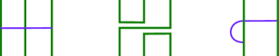
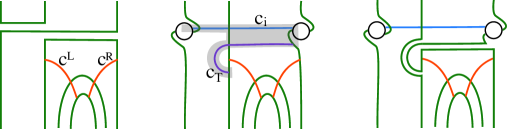
The term bypass rotation is used in several different, but related, senses in the literature. Here, we consider the phenomenon as presented in [HKM07] and recall the proof that it is a consequence of the above two moves. Let be a bypass arc on . Let be another bypass arc as in Figure 3; i.e., subsegments of and together with two segments of cobound a rectangle that is to the right of when is oriented as the boundary of . Let be a neighbourhood of shown shaded in the right hand picture of Figure 3. The arc is said to be a rotation of the bypass arc .
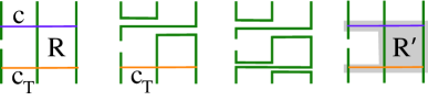
Lemma 2.8.
Suppose that a bypass disc is attached to the arc on some surface , as shown in Figure 3. Then there also exists a bypass disc attached to along . Furthermore, is contained in a neighbourhood of and .
The second claim of the lemma will be useful in the proof of Proposition 3.8 below.
Proof.
The existence claim follows from a formal convex surface theory argument. After a bypass is attached along , is a trivial bypass arc on the new surface. Since trivial bypasses always exist, it follows that there exists a bypass disc attached along . The [TI] move then implies that can be factored as . However, the bypass arcs and are disjoint on , so the associated bypasses commute. Applying the [FC] move gives the factorisation . It follows that the bypass along can be directly attached onto .
The next argument is illustrated in Figure 4.
To construct directly, consider a Legendrian realisation of the arc labeled in Figure 4. Perform a Legendrian isotopy so that is properly embedded in . Since , a regular neighbourhood of this push-off is a contact -handle shown in bold on the first figure. Observe that is attached to along , but the blue disc it cobounds with is not a bypass disc. However, we may isotope this disc across the product disc shown in the centre figure to get a bypass disc cobounded by and . ∎
3. Heegaard Splittings and the Giroux Correspondence
With useful tools and vocabulary established, we now turn to proving the Giroux Correspondence. As a first step, Section 3.1 summarises results from [LV] that allow us to restate the theorem about a pair of open books as a theorem about a pair of Heegaard splittings. Section 3.2 introduces bridging as an operation to stabilise a Heegaard splitting of a contact manifold. After establishing some properties of bridge splittings, we relate them to refinements in Section 3.3 to prove the main result.
3.1. Tight Heegaard splittings and refinement
As described in Section 2.2, each convex Heegaard splitting of a contact manifold corresponds to an open book decomposition supporting the contact structure. Here we recall a key idea from [LV] that extends the class of Heegaard splittings of a contact manifold which determine open books.
Definition 3.1.
The Heegaard splitting of is tight if is convex and the restriction of to each of and is tight.
The definition of a convex Heegaard splitting requires a system of meridional discs each intersecting twice. In contrast, meridional discs in a tight Heegaard splitting may intersect an arbitrary number of times. However, a process called refinement allows us to construct a convex splitting from a tight one.
Refinement was introduced in [LV, Section 5.] . Roughly speaking, refinement stabilises the tight Heegaard splitting by drilling along Legendrian curves embedded in meridional discs. The drilling process cuts each non-product disc into subdiscs, and the curves are chosen so that these subdiscs are product discs for the stabilised Heegaard splitting . See Figure 5. This refinement is necessarily convex, so via Lemma 2.5 one may view refinement as a process which associates an open book decomposition to a tight Heegaard splitting of .
There are choices involved in constructing a refinement (e.g., discs, tunnels), but these preserve the positive stabilisation class of the associated open book.
Theorem 3.2.
[LV, Lemma 3.8 and Theorem 5.10] Suppose that and are refinements of the tight Heegaard splitting . If and are the open book decompositions associated to and , respectively, then and admit a common positive stabilisation.
In light of Theorem 3.2, we define a positive stabilisation of a tight Heegaard splitting as a topological stabilisation of the Heegaard splitting which induces a positive open book stabilisation on the open books associated to the refinements.
This new language permits us to restate the hard direction of the Giroux Correspondence:
Theorem 3.3 (3-dimensional Giroux Correspondence).
Any two convex Heegaard splittings of admit a common positive stabilisation.
Much of the work of [LV] was devoted to showing that various natural operations one may perform on a tight Heegaard splitting are in fact (sequences of) positive stabilisations.
Positive stabilisations may also be characterised directly. Choose an arc properly embedded in one of the handlebodies that is Legendrian isotopic to an arc properly embedded in the closure of . Adding a standard contact neighborhood of this arc to the other handlebody is a positive stabilisation of the original Heegaard splitting. In fact, a related operation has already appeared in the proof of Lemma 2.8. Suppose that in Lemma 2.8 the surface is taken to be a Heegaard surface for a tight Heegaard splitting. In this case, the -handle is a neighbourhood of a Legendrian push-off of , so adding to the handlebody bounded by is a positive stabilisation of the Heegaard splitting.
The proof of Lemma 3.10 in [LV] shows that in a convex Heegaard splitting, attaching any bypass -handle is a positive stabilisation. The following more general statement will be used later.
Theorem 3.4.
[LV, Lemma 7.1] Let and be tight Heegaard splittings of and assume that is obtained from by attaching a single bypass . Let
be the Heegaard splitting formed by attaching only the -handle associated to this bypass. Then the refinements of , and all admit a common positive stabilisations.
Remark 3.5.
Refining a convex Heegaard splitting with respect to a set of product discs preserves the splitting. However, a convex splitting will in general also have non-product meridional discs. Refining with respect to some set of non-product discs will produce a new convex splitting ; then and admit a common positive stabilisation.
3.2. Bridge Heegaard splittings
Given a tight Heegaard splitting , the refinement process described above stabilises to produce a convex Heegaard splitting . In this section we introduce an alternative method to turn any smooth Heegaard splitting into a convex Heegaard splitting . The new Heegaard splitting is called the bridge of .
A bouquet of circles is a skeleton of a handlebody if the handlebody deformation retracts onto the bouquet. When the handlebody is equipped with a contact structure, we may additionally require the bouquet to be Legendrian. Throughout, we will let and denote Legendrian skeletons of and , respectively, and we let and denote their standard neighbourhoods.
Begin with a smooth Heegaard splitting . Since the complement is topologically a product, Theorem 2.6 implies that up to weak contact isotopy, decomposes as a sequence of bypasses attached to .111the triple is called a ”patty” in [HBH]. Attaching only the first bypasses in the sequence determines a new handlebody with convex boundary; letting range over the indices of all bypasses produces a sequence of smoothly isotopic Heegaard surfaces . Each has a bypass arc that determines the bypass . Isotopy of through bypass arcs preserves the weak contact isotopy class of , so we may push each bypass arc off the faces of any -handles already attached.
Definition 3.6.
Let be a bypass decomposition of as above. Define to be the handlebody formed by adding only the bypass -handles to :
Then the bridge of is the Heegaard splitting
Attaching a contact -handle preserves tightness, so it is immediate that is tight. The complementary is also tight, as turning the manifold upside down builds from -handles attached to . In fact, the splitting is convex, as co-core discs for each -handle, together with meridional discs for the neighbourhoods of the skeleta, form a complete set of product discs.
Remark 3.7.
When the original Heegaard surface is already convex in the splitting , one may consider the relative bridge built from a bypass decomposition of , although this need not be convex. Similarly, is constructed from a bypass decomposition of . The relative bridges will be used in Proposition 3.10.
Proposition 3.8.
Up to positive stabilisation, the bridge
is independent of the choice of bypass attaching arcs within their isotopy classes.
Proof.
In order to construct a bridge splitting from a bypass decomposition, all the bypass attaching arcs must be isotoped off the faces of an -handles already attached, but there is no canonical way to perform this isotopy. Although different isotopies preserve the weak contact isotopy type of each , they may produce handlebodies which are inequivalent when the 2-handles are removed. We will show that an isotopy of the attaching -sphere for a -handle on preserves the positive stabilisation class of the bridge .
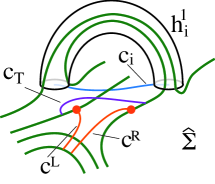
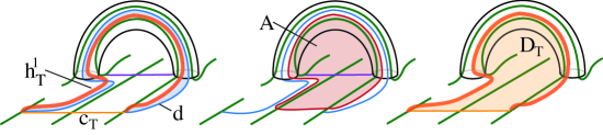
Let and be two bypass attaching arcs for some () that are isotopic on via an isotopy that slides one endpoint across a face of some -handle. Because the proof is local, we may assume without loss of generality that the associated bypass is the most recent one; that is, . See Figure 7. The Heegaard surfaces and associated to attaching bypasses along and , respectively, are not convexly isotopic.
Consider the bypass arc shown on Figure 9. As the endpoints of and can be assumed to be arbitrarily close to , we can also assume that is close to . Thus no other handles are attached on top of and it persists as a bypass arc on . We claim that there is a bypass half-disc attached along in .
Observe that on , the bypass arc is a rotation of . As discussed in Section 2.3, there must exist a bypass disc attached along . Moreover, by Lemma 2.8 may be assumed to lie in a neighbourhood of and the shaded area in the centre picture of Figure 9. It follows that the -handle attached along is disjoint from , so persists in .
Proposition 3.8 implies that up to positive stabilisation, the bridge splitting depends only on , , and the bypass decomposition . As we show next, the bridge is actually independent – again, up to positive stabilisation – of the bypass decomposition.
Proposition 3.9.
Given a smooth Heegaard splitting let and be Legendrian skeletons for and and let . Let and be distinct bypass decompositions of , and let and be the associated bridge Heegaard splittings formed by attaching only the -handles of the respective bypasses to . Then and admit a common positive stabilisation.
Proof.
According to Theorem 2.7, two bypass decompositions of are related by a finite sequence of isotopies, Trivial Insertion moves, and Far Commutation moves. Up to an isotopy that keeps the Heegaard surface convex, Far Commutation preserves the handlebodies and . Thus we only need to show that inserting a trivial bypass preserves the positive stabilisation class of .
Fix a bypass decomposition of . As above, let be the Heegaard splitting formed by attaching the associated -handles to . Now consider an alternative bypass decomposition that differs by the insertion of a trivial bypass attached along a trivial bypass arc somewhere in the sequence, and let denote the associated Heegaard splitting. Observe that the genus of is larger than the genus of because the additional -handle is attached.
We claim that regardless of where the trivial bypass was inserted, and admit a common positive stabilisation. Recall that Proposition 3.8 allows us to isotope each attaching sphere along respective components of while preserving the positive stabilisation class of the bridge splitting. Using this flexibility, ensure that no handle attached after has an attaching sphere that intersects the disc supporting the trivial bypass. Not only can any attaching sphere be isotoped off this region, but we may also impose the stronger condition that subsequent attaching spheres are disjoint from the larger disc shown in Figure 10 that contains the bigon certifying as a trivial bypass arc. As a consequence, remains a trivial bypass arc on ; we will use this below. It follows that we may apply a sequence of Far Commutation moves to get a new bypass decomposition in which the bypass along is attached last.
Attaching along to produces the handlebody . As noted in the comment before Theorem 3.4, adding a bypass -handle to a convex splitting is always a positive stabilisation, which proves the stated claim.
∎
The following two results show that a convex Heegaard splitting and its bridge admit a common positive stabilisation.
Proposition 3.10.
Given a tight Heegaard splitting , let , be Legendrian skeletons for and , respectively. Let be a bypass decomposition of the complement of in , where the index is the order in which the bypass slices are attached to . Let denote the relative bridge splitting with handlebodies and . Then the refinements of the Heegaard splittings and admit a common positive stabilisation.
The relative bridge splitting is tight by construction, so one may flip this Heegaard splitting upside down and apply Proposition 3.10 again to get the following consequence:
Corollary 3.11.
Given a tight Heegaard splitting let , be Legendrian skeletons for and and let be a bypass decomposition of the complement of . Then the bridge splitting and the refinement admit a common positive stabilisation.
The proof of Proposition 3.10 is essentially the same argument as the proof of [LV, Theorem 6.1.]. Since it was not stated in full generality there, we indicate how it follows from the techniques of [LV].
Proof of Proposition 3.10..
Define the sequence of intermediate Heegaard splittings built by attaching only the first of the -handles:
We will show that the refinements of successive Heegaard splittings in this sequence admit common positive stabilisations.
Beginning with the case , construct the refinement of .
Recall that the refinement is constructed by drilling tunnels through meridional discs for the handlebodies. We may choose these discs to be disjoint from the bypass , so adding the -handle to commutes with this drilling. Thus attaching to the refined produces the same Heegaard splitting as taking the refinement of . As noted in Section 3.1, attaching in to in the convex refinement is a positive stabilisation, which completes the base case.
Now proceed by induction on . For the inductive step, note that if is tight, then is also tight because is a proper subset of the tight , while is built from the tight by adding a contact -handle. The argument above shows that refining and then adding a -handle produces the same splitting as first adding the -handle and then refining, which preserves the positive stabilisation class. This establishes the inductive step. ∎
3.3. Proof of the Giroux Correspondence
In order to prove the Giroux Correspondence, we consider a pair of convex Heegaard splittings of a fixed contact manifold. We will modify these Heegaard splittings until they coincide, and each step in this evolution will preserve the positive stabilisation class of the Heegaard splittings.
First, we repeat an argument from the proof of Theorem 6.1 in [LV] that lets us restrict to Heegaard splittings that are smoothly isotopic:
Proposition 3.12.
Any two convex Heegaard splittings of have positive stabilisations that are smoothly isotopic.
Proof.
In the topological setting, the Reidemeister-Singer Theorem asserts that any two Heegaard splittings of a fixed manifold become isotopic after sufficiently many stabilisations. As there are no restrictions on the type of stabilisation that ensure this outcome, we are free to choose positive stabilisation of our convex Heegaard splittings. ∎
Next, we can assume that the skeletons of the Heegaard splittings agree:
Proposition 3.13.
Let and be smoothly isotopic Heegaard splittings of with convex Heegaard surfaces. Then there exist Legendrian skeletons and and an isotopy of keeping convex such that is the skeleton of both and and is the skeleton of both and .
Proof.
Choose a Legendrian bouquet as a skeleton for each handlebody, where . Since is topologically isotopic to , some stabilisations of these bouquets are Legendrian isotopic. As we may stabilise each while preserving it as a skeleton of the respective handlebody, suppose now that the skeletons are Legendrian isotopic to .
Extend this Legendrian isotopy to an ambient contact isotopy of the manifold, . By construction, for all the bouquet is a skeleton for the handlebody with convex boundary , and the analogous statement holds for . Since is an extension of the Legendrian isotopy taking to , we also have that is a skeleton for and is a skeleton for , as desired. ∎
Finally, we are ready to prove the Giroux Correspondence for an arbitrary contact -manifold.
Proof of Theorem 3.3.
Let and be two convex Heegaard splittings of . By Proposition 3.12 we may assume that these Heegaard decompositions are smoothly isotopic. Then Proposition 3.13 implies that after performing an isotopy keeping convex, we may also assume there exist a Legendrian bouquet that is a skeleton of both and and a Legendrian bouquet that is a skeleton of both and .
Choose bypass decompositions of the complement of the skeletons in and :
Concatenating these produces a bypass decomposition of . As usual, let denote the handlebody formed by attaching all of the -handles to . Setting , Corollary 3.11 implies that the refinement and the bridge admit a common positive stabilisation. To complete the argument, we recall Remark 3.5: since is convex, any refinement of is a positive stabilisation of itself. Thus and admit a common positive stabilisation.
Now repeat this process using the alternative Heegaard splitting :
Attaching all – and only – the -handles to gives a new bridge splitting , and a similar argument shows that and admit a common positive stabilisation.
However, and are built from distinct bypass decompositions of , so Proposition 3.9 implies that they also admit a common positive stabilisation, completing the proof. ∎
References
- [Etn04] John B. Etnyre. Convex surfaces in contact geometry : class notes. https://etnyre.math.gatech.edu/preprints/papers/surfaces.pdf, 2004.
- [Gir91] Emmanuel Giroux. Convexité en topologie de contact. Comment. Math. Helv., 66(4):637–677, 1991.
- [Gir02] Emmanuel Giroux. Géométrie de contact: de la dimension trois vers les dimensions supérieures. In Proceedings of the International Congress of Mathematicians, Vol. II (Beijing, 2002), pages 405–414. Higher Ed. Press, Beijing, 2002.
- [HBH] Ko Honda, Joseph Breen, and Yang Huang. The Giroux correspondence in arbitrary dimensions. arXiv:2307.02317.
- [HKM07] Ko Honda, William H. Kazez, and Gordana Matić. Right-veering diffeomorphisms of compact surfaces with boundary. Invent. Math., 169(2):427–449, 2007.
- [HKM09] Ko Honda, William H. Kazez, and Gordana Matić. The contact invariant in sutured Floer homology. Invent. Math., 176(3):637–676, 2009.
- [Hon] Ko Honda. Notes on math 599: contact geometry. https://www.math.ucla.edu/~honda/math599/notes.pdf.
- [Hon02] Ko Honda. Gluing tight contact structures. Duke Math. J., 115(3):435–478, 2002.
- [LV] Joan Licata and Vera Vértesi. Heegaard splittings and the tight Giroux Correspondence. arXiv:2309.11828, to appear in The Journal of Symplectic Geometry.
- [Mas14] Patrick Massot. Topological methods in 3-dimensional contact geometry. In Contact and symplectic topology, volume 26 of Bolyai Soc. Math. Stud., pages 27–83. János Bolyai Math. Soc., Budapest, 2014.
- [Ozb11] Burak Ozbagci. Contact handle decompositions. Topology Appl., 158(5):718–727, 2011.
- [Tia] Bin Tian. Generators and relations of contact categories. PhD thesis.
- [Tor00] Ichiro Torisu. Convex contact structures and fibered links in 3-manifolds. Internat. Math. Res. Notices, (9):441–454, 2000.
- [TW75] W. P. Thurston and H. E. Winkelnkemper. On the existence of contact forms. Proc. Amer. Math. Soc., 52:345–347, 1975.