Exploiting the Semantic Knowledge of Pre-trained Text-Encoders for Continual Learning

Abstract

Deep neural networks (DNNs) excel on fixed datasets but struggle with incremental and shifting data in real-world scenarios. Continual learning addresses this challenge by allowing models to learn from new data while retaining previously learned knowledge. Existing methods mainly rely on visual features, often neglecting the rich semantic information encoded in text. The semantic knowledge available in the label information of the images, offers important semantic information that can be related with previously acquired knowledge of semantic classes. Consequently, effectively leveraging this information throughout continual learning is expected to be beneficial. To address this, we propose integrating semantic guidance within and across tasks by capturing semantic similarity using text embeddings. We start from a pre-trained CLIP model, employ the Semantically-guided Representation Learning (SG-RL) module for a soft-assignment towards all current task classes, and use the Semantically-guided Knowledge Distillation (SG-KD) module for enhanced knowledge transfer. Experimental results demonstrate the superiority of our method on general and fine-grained datasets. Our code can be found in https://github.com/aprilsveryown/semantically-guided-continual-learning.

1 Introduction

Alarge variety of algorithms were proposed to mitigate forgetting in continual learning, employing approaches such as rehearsal-based methods [1, 2, 3, 4], regularization-based techniques [5, 6, 7], and architecture-based solutions [8, 9, 10, 11, 12]. The emergence of Vision Transformers (ViTs) [13] has substantially enhanced the representation capabilities of pre-trained vision encoders for downstream tasks. A number of recent studies, including L2P [14] and DualPrompt [15], have leveraged the potential of pre-trained vision encoders in the context of continual learning, employing a prompt-based learning strategy. However, these works have exposed a notable limitation: performance degradation occurs when the pre-trained dataset exhibits a substantial semantic gap compared to the downstream data [16, 17].

Large scale pre-trained vision-language models, for instance ViT-BERT [18], CLIP [19] and UNITER [20], have emerged as powerful tools that combine computer vision and natural language processing, enabling machines to comprehend visual and textual information. These models can serve as strong foundation models for continual learning, as they were trained on massive datasets, allowing them to learn intricate patterns and relationships between images and language. As mentioned, the continual learning community has focused on applying foundational vision backbones [14, 15, 21], however, less effort has been invested in how to best exploit the rich semantic knowledge contained in the language encoders. A recent exception is Continual-CLIP [22] which shows impressive results in continual learning using both the vision and language encoder of the CLIP model. However, they keep the CLIP model frozen, thereby limiting the generalization to new tasks. In Fig. 1(a), we present an overview of several methods, each characterized by a distinct training strategy. The performance evaluations are shown in Fig. 1(b). The use of pre-trained vision encoders has resulted in incremental performance gains. Interestingly, we will show that better exploitation of the knowledge contained in language encoders can lead to considerable performance improvements.

Method	Language	Vision	Trainable
DER[11]	x	scratch	yes
DyTox++[9]	x	scratch	yes
L2P[14]	x	pre-trained	yes
DualPrompt[15]	x	pre-trained	yes
Continual-CLIP[22]	pre-trained	pre-trained	no
CoOp[23]	pre-trained	pre-trained	yes
Ours	pre-trained	pre-trained	yes

(a)

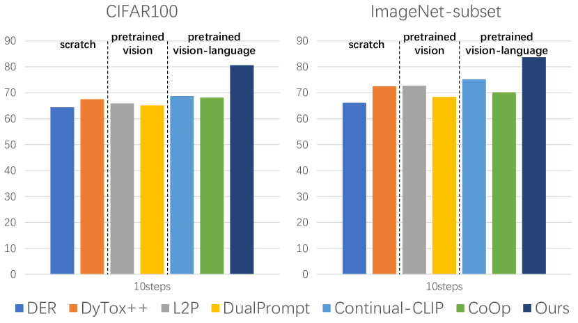
(b)

Figure 1: (a) Comparison of different models. (b) Performance comparison using different models across two datasets.

Establishing similarity between objects is a fundamental aspect of human perception and cognition, as highlighted by previous research [24]. pre-trained language models provide access to the semantic similarity between classes. In this paper, we propose two techniques to exploit the rich semantic information of pre-trained language models. Firstly, we exploit the intra-task semantic relationships between class labels. Instead of only using the available ground truth label to train on the newly arriving data, we replace the label with a soft-assignment towards all current task classes based on intra-task semantic relations. This ensures that each sample contributes to aligning the vision backbone with respect to multiple semantic classes. Secondly, we propose to exploit the inter-task semantic relationships between old and new classes to improve stability during continual learning. For example, current class data for ‘motor bikes’ is expected to assign part of its prediction to the related previous task class of ‘bikes’ thereby preventing forgetting of previous classes. These inter-task relationships, derived from the language encoder, are used in a semantically-guided knowledge distillation technique.

To summarize, the main contributions of the paper are:

• The usage of pre-trained models in continual learning has focused on pre-trained vision encoders. We show that exploiting the semantic information of the data labels with pre-trained language encoders can greatly enhance the accuracy of continual learning.

• We extend the existing image distillation method based only on visual information with a term that exploits the knowledge of the labels of the current data with respect to the classes of previous tasks (inter-task semantic similarity). This improvement, called SG-KD, is shown to significantly increase the efficiency of distillation (and reduce catastrophic forgetting). In addition, we show how to exploit the intra-task semantic similarity (called SG-RL).

• Extensive experimental results show that our approach surpasses all methods by a substantial margin on several datasets under both many-shot and few-shot settings. Results on CIFAR100 under the 10-step setting show that the proposed method can greatly improve the accuracy after the last task with 11.4 points compared to the state-of-the-art.

2 Related Work

2.1 Continual Learning

Continual learning research has witnessed significant advancements in recent years, resulting in the development of three main categories of approaches: rehearsal-based, regularization-based, and architecture-based. Rehearsal-based methods store previous task exemplars or generate fake exemplars using generative models to combat catastrophic forgetting. iCaRL [3] combines exemplar rehearsal with knowledge distillation, UCIR [2] addresses classification bias through normalization, and WA [4] ensures consistency in weight vector norms between old and new classes. Regularization-based methods impose constraints on network parameters, with strategies such as estimating parameter importance (EWC [5]) and distilling output from old and new models (LwF [6]) to retain information about previous tasks. SDC [25] proposed compensating the feature drift to prevent forgetting on some regularization-based continual learning methods. Architecture-based methods assign specified parameters to tasks or dynamically expand the network architecture. HAT [10] blocks and activates specific parts for old tasks, while DER [11] utilizes task-specific feature extractors and tackles parameter growth through pruning. Transformer-based continual learning paradigms, like DyTox [9], utilize shared self-attention layers and task-specific tokens to achieve task-specialized embeddings.  [26] proposed to apply Masked Autoencoders (MAEs) for continual learning and introduced a bilateral MAE framework that integrates learning from both image-level and embedding-level.  [21] proposed to adaptively assign distillation loss weights by evaluating the relevance of each patch to the current task.

2.2 Continual Learning with Foundation Models

A recent emerging trend in the field of continual learning is to combine pre-trained vision transformers with parameter-efficient fine-tuning techniques to continuously adapt the model to a stream of incoming downstream tasks. Specifically, these techniques involve prompt tuning [27, 28], prefix tuning [29], Adapter[30, 31], LoRA [32] , etc. The core of applying such a technique to continual learning is to construct additional learnable parameters or modules to instruct pre-trained representations and select appropriate prompts during inference time. L2P [14] optimizes the cosine similarity between query features and learnable keys, the most relevant prompts are selected and prepended to the token sequence both during training and inference. DualPrompt [15] further subdividing the prompts into general prompts sharing across all tasks and expert prompts picked and optimized in the same way as [14]. CODAPrompt [33] proposes to reweight prompts through input-conditioned weights, facilitating end-to-end optimization of the query-key mechanism across tasks. Distinct from the aforementioned prompt-based approaches, another line of work aims to construct classifiers through the extraction of robust feature representations via pretrained models. SLCA [17] fine-tuned the full pretrained model and recommended using different learning rates for the representation layers and the classifier to address the forgetting problem in representation layers, they further incorporated prototype replay for post-hoc alignment of the classification layers to reduce bias in the classifier. RanPAC [34] suggested employing a frozen random projection layer to project pretrained features into a high-dimensional space, thereby improving linear separability, they additionally utilize an online LDA classifier to eliminate correlations between categories. EASE [35] proposed to employ distinct adapters for each task to acquire task-specific features, and construct a unified classifier by synthesizing prototypes for old classes through semantic relevance.

2.3 Pre-trained Vision-Language Model

Large-scale vision-language pre-trained models like CLIP [19] and ALIGN [36] have emerged as powerful tools for representation learning due to their high transferability. Numerous studies [37, 38, 23] have focused on adapting these models to downstream tasks. For instance, CoOp [23] proposed vectorizing prompts, keeping the CLIP model fixed while optimizing only the prompt vectors. However, it was observed in[38] that prompts learned using this method exhibited poor generalization performance on unseen classes. To address this limitation, they introduced a meta-net to generate an input-conditional token for each image. Some works attempt to simultaneously optimize visual and textual prompts to improve the adaptability of vision-language models for downstream tasks. MaPLe [39] proposed to promote strong coupling between prompts of two different modalities to improve the consistency between visual and linguistic representations. PromptSRC [40] designed a regularization framework when training models on downstream tasks to prevent overfitting, which enhances the generalization capacity of the model. Differing from prompt-based approaches, some works try to incorporate adapters with MLPs into the transformer architecture to capture task-specific information. CLIP-adapter [41] introduced extra bottleneck layers for learning new features. While these approaches have demonstrated significant improvements on various tasks compared to the adapted results provided by CLIP [19], they all shared the common limitation of freezing all the pre-trained parameters.

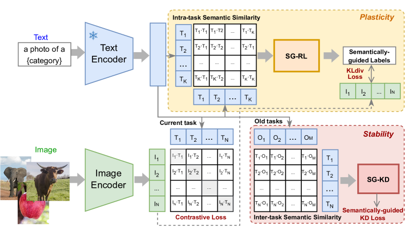
Figure 2: An overview of the proposed framework. We update the image encoder part of the CLIP model and train it with contrastive loss. We integrate semantic information into two modules: The SG-RL module, represented by the yellow block of the framework, aims to learn more discriminative representation to improve the model plasticity based on the intra-task semantic similarity. We train the model with KL-divergence loss between the generated semantically-guided labels and the original predictions. The SG-KD module, represented by the pink block of the framework, exploits the semantic similarity between current and previous task labels for knowledge distillation, to consolidate the model stability.

3 Preliminary of CLIP model

Here we explain the details of the CLIP model. Let $I$ denote the set of normalized image features encoded by the image encoder, and $T$ denote the set of corresponding normalized text features. Assume that we have $N$ samples, the logits for each image-text pair are computed as follows:

$$P_{i,j}=\beta\cdot I_{i}\cdot T_{j}^{\top},$$ (1)

where $\beta$ is a learned scalar, $P_{i,j}$ is the cosine similarity score between the $i$th image and the $j$th text, and $i\in\{1,\dots,N\}$ and $j\in\{1,\dots,N\}$ are indices for the images and texts, respectively. Then the loss for each modality can be expressed as:

$$L_{image}=-\frac{1}{N}\sum_{i=1}^{N}\log\left(\frac{\exp(P_{i,i})}{\sum_{j=1}^{N}\exp(P_{i,j})}\right),$$ (2)

$$L_{text}=-\frac{1}{N}\sum_{j=1}^{N}\log\left(\frac{\exp(P_{j,j})}{\sum_{i=1}^{N}\exp(P_{i,j})}\right)$$ (3)

The overall loss of the CLIP model is the sum of the image loss $L_{image}$ and text loss $L_{text}$, which are averaged over the the number of samples. It can be represented as:

$$L_{c}=\frac{1}{2}(L_{image}+L_{text})$$ (4)

The loss function is minimized during pre-training to learn the joint representations of images and texts where semantically similar pairs are closer together and dissimilar pairs are farther apart.

The CLIP model has demonstrated remarkable continual learning performance without any fine-tuning [22]. To enhance its performance on new tasks and adapt to evolving data distributions over time, we thus propose to fine-tune the last block of the vision encoder. We aim to leverage the strong generalization ability of the CLIP model while also updating its representation to better adapt to incoming data.

4 Method

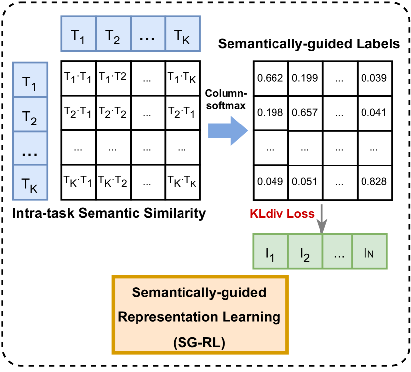
(a) Illustration of SG-RL module.

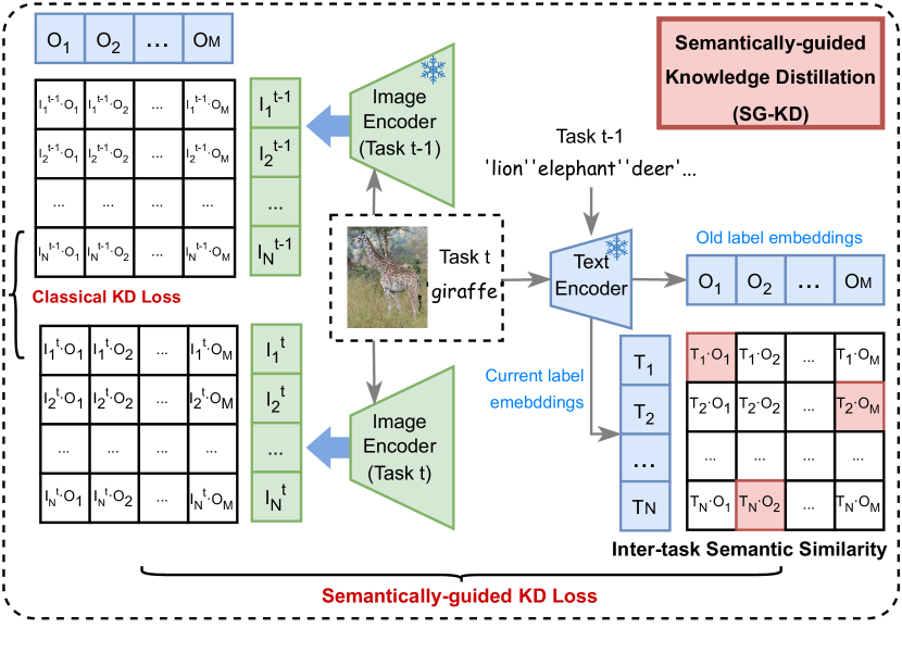
(b) Illustration of SG-KD module.

Figure 3: An illustration of two components. (a) The SG-RL module calculates the text embedding similarity between the current labels using a pre-trained text encoder. It then generates semantically-guided labels that are more informative. (b) The SG-KD module constructs an inter-task similarity matrix based on text embeddings of previous and current task class labels. The most similar categories of the current class from old classes are selected by computing row-wise maximums (pink cells). The similarity value is added to the previous model’s prediction logits at the most similar position, and the rest are subtracted from in each row. The enhanced logits are used for knowledge distillation between the current and previous models.

To overcome the challenges of catastrophic forgetting during the training of pre-trained models, we introduce a novel approach that integrates semantic information guidance into the process of continual knowledge learning, as shown in Fig. 2. Leveraging the power of well-trained text embeddings, our proposed approach facilitates efficient interaction within and across task labels, leading to improved performance from two crucial perspectives. Firstly, we focus on learning more informative representations for new data by leveraging intra-task semantic similarity, thereby enhancing model plasticity (SG-RL module). Secondly, we establish a relationship between old and new tasks by incorporating inter-task semantic similarity during the model distillation process, ensuring stability (SG-KD module). In the following sections, we introduce these two components and explain how they work.

4.1 Intra-task Semantically-Guided Representation Learning (SG-RL)

As shown in the yellow part of Fig. 2, assume we have $K$ classes contained in the current task $t$, their labels can be denoted as $C^{t}$=$\{c^{t}_{1},c^{t}_{2},\cdots,c^{t}_{K}\}$(for simplicity, we omit the superscript $t$ in the following descriptions). We encode the text embeddings of these labels by the pre-trained language part of CLIP to obtain the normalized text embeddings $\mathbf{T}^{t}=\{T_{1},T_{2},\cdots,T_{K}\}$, where $||T_{k}||=1$ and $k\in\{1,2,\cdots,K\}$. After obtaining the text embeddings of the current labels, we acquire the intra-task semantic similarity by computing the cosine similarity between each pair of text embeddings. This yields a text similarity matrix $\mathbf{S}^{t\leftrightarrow t}$ which represents the intra-task similarity between the $i$-th and $j$-th labels; it can be described as follows:

$$S_{i,j}^{t\leftrightarrow t}=[T_{i}^{\top}T_{j}]_{K\times K},(i,j\in\{1,2,\cdots,K\}),$$ (5)

This similarity score contains the pairwise similarity within each category within the current task.

To further convert the one-hot labels to our informative semantically-guided labels $C^{sg}=[C_{i,j}^{sg}]_{K\times K}$, we compute the softmax function over each column of $\mathbf{S}^{t\leftrightarrow t}$ with a parameter $\alpha$ which controls the degree of softness of the generated labels as follows:

$$C_{i,j}^{sg}=\frac{\exp(\alpha\cdot S_{i,j}^{t\leftrightarrow t})}{{\textstyle\sum_{k=1}^{K}\exp(\alpha\cdot S_{i,k}^{t\leftrightarrow t})}}$$ (6)

The semantically-guided labels $C^{sg}$ encode the relationships and similarities between categories, allowing for a more comprehensive representation of class associations within the current task.

We then compute the KL-divergence loss $\mathcal{L}_{SG-RL}$ between $\hat{y}_{i,j}$ and the semantically-guided labels $C^{sg}_{i,j}$:

$$\mathcal{L}_{SG-RL}=D_{KL}(\hat{y}||C^{sg})=\sum_{i=1}^{N}\sum_{j=1}^{K}\hat{y}_{i,j}\cdot\log\frac{\hat{y}_{i,j}}{C_{i,j}^{sg}},$$ (7)

where the logits $P^{t}=[P_{i,j}^{t}]_{N\times K}$ of $N$ images in current task is computed by Eq. 1, and the prediction score $\hat{y}_{i,j}=\log\frac{\exp(P_{i,j}^{t})}{\sum_{k=1}^{K}\exp(P_{i,k}^{t})}$ is after applying the log-softmax.

The detailed illustration of the SG-RL model is shown in Fig. 3(a). We propose to exploit the semantic knowledge of the pre-trained text-encoder by means of the intra-task semantic similarity between class labels (see Eq. 5). We replace the one-hot ground truth label in the cross entropy with a soft-assignment towards all current task classes. As a consequence, each sample contributes to aligning the vision backbone with respect to multiple semantic classes, leading to higher plasticity.

4.2 Inter-task Semantically-Guided Knowledge Distillation (SG-KD)

In this section, we aim to exploit the semantic knowledge of the pre-trained text-encoder to prevent forgetting and improve stability of the continual learner. Our main insight is that the semantic similarity between current and previous task labels can be exploited to prevent forgetting. For example, the current task label ‘truck’ can be used to prevent forgetting of previous related class labels like ‘bus’. As shown Fig. 3(b), given an image $x_{i}$ of the current task, the image features encoded by the previous image encoder are denoted as $I^{t-1}_{i}$, and the corresponding normalized text embeddings of old-class labels $y^{t-1}$ can be encoded by the pre-trained text encoder as $O_{j}$. Thus, the prediction logits $P^{t-1}=[P^{t-1}_{i,j}]_{N\times M}$ (the number of old classes is $M$) of current data on the previous image encoder is computed as:

$$P^{t-1}_{i,j}=\beta\cdot I^{t-1}_{i}\cdot O_{j}^{\top},(i\in{1,2,\dots,N},j\in{1,2,\dots,M})$$ (8)

The prediction logits of the current image encoder on old-class heads $P^{t}=[P^{t}_{i,j}]_{N\times M}$ are:

$$P^{t}_{i,j}=\beta\cdot I^{t}_{i}\cdot O_{j}^{\top},$$ (9)

which can be used to compute a prediction over the labels:

$$p^{t}(y^{t-1}_{j}|x_{i})=\frac{\exp(P_{i,j}^{t})}{\sum_{j}\exp(P_{i,j}^{t})}$$ (10)

and similarly for $p^{t-1}(y^{t-1}_{j}|x_{i})$; the difference is that this probability is based on the model at time $t\text{-}1$. Traditional knowledge distillation [6, 3] between the old and current model can be described as follows:

$$\mathcal{L}_{KD}=D_{KL}(p^{t}(y^{t-1}|x_{i}),p^{t-1}(y^{t-1}|x_{i})).$$ (11)

Our contribution is that we aim to improve this distillation by also including the knowledge of the current sample labels about the previously seen classe in the distillation. Therefore, we use the semantic relationship between the current categories $y^{t}$ and the previous categories $y^{t-1}$, without requiring access to any visual information. We introduce Semantically-guided Knowledge Distillation (SG-KD); the loss for an image $x_{i}$ is given by:

$$\begin{split}\mathcal{L}_{SG-KD}=D_{KL}(p^{t}(y^{t-1}|x_{i}),p^{t-1}(y^{t-1}|x_{i}))\\ +\mu D_{KL}(p^{t}(y^{t-1}|x_{i}),s(y^{t-1}|y_{c_{i}}^{t}))\end{split}$$ (12)

where $y^{t}_{c_{i}}$ refers to the image label of image $x_{i}$. The first term on the right-hand site is the same as in Eq. 11. The second term provides us the distillation between $s(y^{t-1}|y_{c_{i}}^{t})$ and the current predictions. $\mu$ is the tradeoff between these two distillation losses. We derive $s(y^{t-1}|y^{t}_{c_{i}})$ from the inter-task semantic similarity $\mathbf{S}^{{t-1}\leftrightarrow t}$ between the text embeddings of current task labels $T$ and the old task labels $O$ as follows:

$$S_{i,j}^{{t-1}\leftrightarrow t}=T_{i}\cdot O_{j}^{\top}$$ (13)

Here $S_{i,j}^{{t-1}\leftrightarrow t}$ provides a measure of similarity between classes from different tasks. This allows the model to capture the semantic relationships between tasks and leverage this information for knowledge transfer. Thus, $s(y^{t-1}|y^{t}_{c})$ can be computed as:

$$s(y^{t-1}_{j}|y^{t}_{c_{i}})=\frac{\exp(S_{i,j}^{{t-1}\leftrightarrow t}/\tau)}{\sum_{j}\exp(S_{i,j}^{{t-1}\leftrightarrow t}/\tau)}$$ (14)

$\tau$ is a hyper-parameter representing the temperature in the softmax function.

The final objective function can be described as follows:

$$\mathcal{L}=\mathcal{L}_{c}+\lambda_{1}\mathcal{L}_{SG-RL}+\lambda_{2}\mathcal{L}_{SG-KD},$$ (15)

where $\lambda_{1}$ and $\lambda_{2}$ are trade-offs between the contrastive loss $\mathcal{L}_{c}$, KL-divergence loss $\mathcal{L}_{SG-RL}$ and the semantically-guided distillation loss $\mathcal{L}_{SG-KD}$.

5 Experiments

5.1 Experimental Settings

TABLE I: Details of all datasets used in this paper.

Datasets	#Classes	Train size	Test size
CIFAR100 [42]	100	50000	10000
imagenet_subset [43]	100	129395	5000
miniImageNet [43]	100	50000	10000
ImageNet1000 [43]	1000	1281167	50000
Food-101 [44]	101	75750	25250
Stanford Cars [45]	196	8144	8041
FGVC Aircraft [46]	100	6667	3333
Oxford-IIIT pets	37	3680	3669
Caltech-101 [47]	102	3060	6085
Oxford Flowers 102 [48]	102	2040	6149
CUB-200-2011 [49]	200	5994	5794
Stanford Dogs [50]	120	12061	8519

TABLE II: The results on CIFAR100 are averaged over three class orders (seeds) under 10, 20, and 50 steps, following the setting proposed in [9]. The bold parts represent the best results, underlined parts indicate the second best, and up arrows show the improvement of the best over the second best. Re-implemented results are marked with an asterisk (*) .

CIFAR100	10 steps			20 steps			50 steps
Methods	#Param.	Avg	Last	#Param.	Avg	Last	#Param.	Avg	Last
Linear probe	-	-	83.1	-	-	83.1	-	-	83.1
Joint	7.09	-	83.9	7.09	-	83.9	7.09	-	83.9
UCIR [2]	11.22	58.7	43.4	11.22	58.2	40.6	11.22	56.9	37.1
BiC [51]	11.22	68.8	53.5	11.22	66.5	47.0	11.22	62.1	41.0
WA [4]	11.22	69.5	53.8	11.22	67.3	47.3	11.22	64.3	42.1
PODNet [8]	11.22	58.0	41.1	11.22	54.0	35.0	11.22	51.2	33.0
DER w/o p [11]	112.27	75.4	65.2	224.55	74.1	62.5	561.39	72.4	59.1
DER [11]	-	74.6	64.4	-	74.0	62.6	-	72.1	59.8
DyTox++ [9]	10.73	77.0	67.5	10.74	76.8	64.3	10.77	75.5	59.5
Continual-CLIP[22]	-	-	68.7	-	-	68.7	-	-	68.7
CoOp∗[23]	7.91	76.2	68.1	7.91	77.0	67.6	7.91	78.3	66.3
CoCoOp∗[38]	7.13	75.1	65.9	7.13	75.1	63.1	7.13	74.8	61.1
L2P∗[14]	7.38	76.3	65.9	7.38	75.2	66.2	7.38	76.5	64.6
DualPrompt∗[15]	7.42	71.3	65.1	7.42	66.2	65.4	7.42	70.1	66.6
Ours	7.09	86.6 ($\uparrow$9.6)	80.1 ($\uparrow$11.4)	7.09	86.0 ($\uparrow$9.0)	78.2 ($\uparrow$9.5)	7.09	81.8 ($\uparrow$3.5)	74.1 ($\uparrow$5.4)

TABLE III: We compare the results obtained on the imagenet_subset dataset (100 classes) and the ImageNet full dataset (1000 classes), where the training session is split into 10 steps, with each step containing an equal number of classes for each task.

Methods	imagenet_subset 10 steps					ImageNet1000 10 steps
	#Param.	top-1		top-5		#Param.	top-1		top-5
		Avg	Last	Avg	Last		Avg	Last	Avg	Last
Linear probe	-	-	83.9	-	97.6	-	-	80.2	-	94.1
Joint	7.09	-	86.1	-	98.3	7.09	-	81.1	-	96.5
DER w/o p[11]	112.27	77.2	66.7	93.2	87.5	116.89	68.8	60.2	88.2	82.9
DER[11]	-	76.1	66.1	92.8	88.4	-	66.7	58.6	87.1	81.9
DyTox++[9]	11.01	80.8	72.5	94.4	90.1	-	-	-	-	-
Continual-CLIP[22]	-	-	75.2	-	96.9	-	-	68.6	-	90.6
CoOp∗[23]	7.91	80.9	70.2	97.5	94.5	15.28	75.2	66.7	95.9	91.9
CoCoOp∗[38]	7.13	81.8	71.0	98.5	96.1	7.13	64.6	56.0	92.3	88.7
L2P∗[14]	7.38	82.2	72.7	98.5	96.4	8.07	71.9	63.3	95.0	90.4
DualPrompt∗[15]	7.42	79.6	68.4	97.7	95.0	8.11	70.7	64.0	94.4	92.1
Ours	7.09	89.8 ($\uparrow$7.6)	83.1 ($\uparrow$7.9)	99.1 ($\uparrow$0.6)	98.4 ($\uparrow$1.5)	7.09	83.4 ($\uparrow$8.2)	75.1 ($\uparrow$6.5)	97.4 ($\uparrow$1.5)	95.2 ($\uparrow$3.1)

5.1.1 Dataset and task spilt.

Our experimental evaluation begins by conducting experiments on three datasets that are commonly used for continual learning scenarios: CIFAR100 [42], imagenet_subset, and ImageNet1000  [43]. For CIFAR100, we adopt the incremental phase splitting into 10, 20, and 50 steps, following the approach of DyTox [9]. In each split, we further assess the performance of the proposed method under three different class orders. Regarding imagenet_subset and ImageNet1000, we split the incremental phase into 10 steps, with 10/100 new classes added at each incremental step. We further evaluate the performance on eight fine-grained datasets. We also evaluate for few-shot continual learning on miniImagenet, and CUB-200-2011 following [52, 53]. For miniImagenet, we split the 100 classes into 60 base classes and 40 classes across 8 sessions with 5 new classes per session. CUB-200-2011 is divided into 100 base classes and 100 classes across 10 sessions with 10 new classes per session. Each incremental session for all three datasets consists of 5 training samples per new class.

The dataset splits follow two patterns: in the $A+B\times C$ split, $A$ represents the number of classes in the initial task, $C$ indicates the total number of steps, and $B$ signifies the number of new classes added at each incremental stage; for the $A\times B$ split, $A$ new classes are introduced in each of the $B$ incremental steps. Note that we handle the Oxford-IIIT pets dataset separately due to its 12 cat categories and 25 dog categories, splitting it into two stages: one for cats and another for dogs. The details of all datasets are listed in Table I.

5.1.2 Implementation details.

All experiments were conducted with a vision backbone of ViT-B/16 version CLIP model. We train every task for 10 epochs except for CUB and Aircrafts with 20 epochs. We adopt SGD in all experiments as the optimizer with an initial learning rate of 0.01(0.001 for few-shot setting), weight decay is 2e-4 and 0.9 for momentum. Batch size is 256 for all experiments. We set $\alpha$ to 13 in Eq. 6, $\beta$ is set to 100 in Eq. 8 following [22] and $\tau$ to 0.1 in Eq. 14 for all datasets. The trade-off parameters, $\lambda_{1}$ and $\lambda_{2}$, are set to 0.5 and 0.1 across all datasets (the hyper-parameters sensitive experiments can be found in Section 5.4.5 ). We save 20 exemplars for each old class by herding algorithm in all experiments except the ablation on different exemplar sizes (in Section 5.4.4), following the setting in [9, 3, 11]. Under the few-shot setting, none exemplar is saved following the setting in [52, 53]. To ensure fairness, methods trained with a pre-trained model are initialized with CLIP. For implementing ‘Linear Probe’, we directly add a fully connected layer after the linear projection, we train 100 epochs for each dataset with an initial learning rate of 0.1 and decays by 0.1 every 45 epochs. For ‘Joint’, to ensure fairness in comparison, we fine-tune the last block of the network for joint training, all training samples are acquired concurrently in the same session. We train 100 epochs for each dataset with an initial learning rate of 0.01 and decays by 0.1 every 45 epochs.

For all experiments in the paper, we applied RandomResizedCrop, RandomHorizontalFlip and normalization for data augmentation. The random seed was set to 1993 except when spliting CIFAR100 with three different class orders as shown in Table 2. We use randomly generated integers ranging from 1 to 5000 for the other two class orders.

Test-time evaluation details: For each test sample $x_{\text{test}}$, the image is passed through the image encoder, resulting in its image feature $I_{\text{test}}$. Meanwhile, we collect all previously seen categories as prompts and feed them to the text encoder to obtain the text features $T=\left\{T^{i};1\leq i\leq k\right\}$, where $k$ is the number of seen classes. Then we compute the cosine similarity between image feature and text features:

$$s_{i}=\frac{I_{test}\cdot T_{i}}{\left\|I_{test}\left\|\cdot\right\|T_{i}\right\|}$$ (16)

where $1\leq i\leq k$, the prediction score for $x_{test}$ can then be computed as:

$$p=\frac{\exp(s_{i})}{{\textstyle\sum_{i=1}^{k}}\exp(s_{i})}$$ (17)

The class with the highest predicted score is considered as the predication.

TABLE IV: Results on eight fine-grained datasets with different task splits.

Dataset	Food	Cars	Aircraft	Pets	Caltech	Flowers	CUB	Dogs
#classes	101	196	100	37	102	102	200	120
split	11+$9\times 10$	$28\times 7$	$10\times 10$	12+25	$17\times 6$	$17\times 6$	$20\times 10$	$12\times 10$
Linear probe	92.8	86.7	59.5	93.1	94.7	98.1	80.4∗	78.6∗
Joint	93.1	91.5	73.2	94.7	93.8	98.1	85.0	80.6
Continual-CLIP[22]	89.2	65.6	27.1	88.9	89.3	70.4	55.6∗	63.4∗
CoOp∗[23]	84.6	86.1	57.6	94.0	90.2	97.0	80.1	75.8
CoCoOp∗[38]	79.1	84.9	59.8	92.8	88.2	97.2	77.0	69.7
L2P∗[14]	81.7	86.9	61.1	92.8	88.6	97.0	82.6	75.9
DualPrompt∗[15]	80.5	82.7	45.5	90.6	86.4	96.7	79.6	70.3
Ours	90.9 ($\uparrow$1.7)	88.6 ($\uparrow$2.5)	66.6 ($\uparrow$5.5)	94.0	92.3 ($\uparrow$2.1)	96.2	83.7 ($\uparrow$1.1)	79.6 ($\uparrow$3.7)

5.2 Full-shot Continual Learning Setting

5.2.1 Evaluation on general datasets.

We conducted extensive experiments on three benchmark datasets, namely CIFAR100, imagenet_subset, and ImageNet1000 in comparison to state-of-the-art approaches. In Table II, we present the averaged accuracy on CIFAR100 over three different class orders and three different splits. In the most common 10-step split, our method achieves an impressive accuracy of 80.1 after the last incremental step, surpassing the previous state-of-the-art method by 11.4 points. Even for longer task sequences of 20 or 50 steps, our method consistently maintains superior performance, with at least 9.5 and 5.4 points higher accuracy than the state-of-the-art ‘Last’ result respectively. Moving to larger-scale continual learning scenarios, as shown in Table III, our method demonstrates even greater superiority. On imagenet_subset dataset, we outperform the state-of-the-art result by 7.9 points in terms of top-1 ‘Last’ accuracy, approaching the performance of linear probing [19]. Furthermore, on the challenging ImageNet1000 dataset, our method achieved significant improvements with a 6.5-point increase in top-1 ‘Last’ accuracy and a 3.1-point increase in top-5 accuracy. Overall, our experimental results demonstrate that the proposed method consistently outperforms state-of-the-art approaches on all three datasets, showcasing its superior performance and stability in continual learning settings.

Figure 4: The accuracy change during few-shot incremental training sessions on CUB-200-2011 and miniImageNet datasets.

TABLE V: The effect of different components. ‘FT’ represents only applying contrastive loss for training, ‘One-hot Label’ utilizes the prompt of each class as a classification head during training, and uses the one-hot encoded labels to calculate the cross-entropy loss. ‘Naive KD’ distills the output of the current data between old and new models with the KD loss proposed in[54] (ref Eq. 11).

	FT	One-hot Label	SG-RL(Eq. 6)	Naive KD(Eq. 11)	SG-KD(Eq. 12)	CIFAR100 10 steps	imagenet_subset 10 steps
C-CLIP[22]						68.7	75.2
	✓					75.7	81.1
	✓	✓				71.4	75.2
	✓		✓			77.0	81.8
	✓		✓	✓		77.7	82.6
	✓		✓		✓	80.6	83.1

5.2.2 Evaluation on fine-grained datasets.

To further validate the effectiveness of the proposed method, we conduct experiments on eight fine-grained datasets. In fine-grained datasets, all categories belong to the same parent category in a hierarchical relationship, which intuitively indicates a high degree of semantic similarity among them, which is more challenging. In Table IV, we present the performance of our proposed method compared to other methods on different splits of the datasets. We notice that the Continual-CLIP evaluation on datasets like Cars, Aircrafts, and CUB, is initially poor. State-of-the-art methods obtain a substantial improvement, particularly on Aircraft where the gain reaches 34 points with L2P. Our method achieves performance very close to the joint training results, with a gap of less than 1 point on multiple datasets such as Pets and Dogs. Moreover, our method even surpasses the results of linear probing evaluation on multiple datasets, which is typically used to assess the quality of pre-trained features.

5.3 Few-shot Continual Learning Setting

Our proposed method has demonstrated impressive results on several datasets, including coarse and fine-grained datasets. It is interesting to evaluate its effectiveness under the few-shot continual learning setting, which poses a significant challenge. In this setting, the model needs to quickly adapt to new classes with limited labeled data while preserving knowledge of previous tasks. We present dynamic accuracy curves that showcase the incremental training sessions on the CUB-200-2011 and miniImageNet datasets in Fig. 4. The curves highlight the notable performance of our method (shown in red) as it significantly outperforms state-of-the-art approaches with (in solid line) and without (in dashed line) ViT backbone by a substantial margin over all incremental sessions. Particularly on the miniImageNet dataset, our method achieves a final accuracy about 36.5 points higher than FACT and 5.3 points higher than CoOp.

5.4 Ablation Study

5.4.1 Components of our proposed method

We conduct ablation experiments on CIFAR100 and imagenet_subset to thoroughly examine the effect of the different proposed modules. Both datasets were split into 10 steps, and the results are shown in Table V. On both datasets, the contrastive loss significantly improves the final accuracy compared to Continual-CLIP. However, when we additionally apply the one-hot encoded labels to add an auxiliary classification loss, we observe a significant performance drop. By incorporating our ‘SG-RL’ module, the model shows a gain of 1.3 points on CIFAR100 and 0.7 points on imagenet_subset. Furthermore, when we apply knowledge distillation to the loss function, our proposed ‘SG-KD’ demonstrates superior performance over ‘Naive KD’ (ref Eq. 11) on both datasets, with a particularly notable gain of 2.9 points on Cifar100.

TABLE VI: Comparison of different vision models on CIFAR100 and imagenet_subset, learned with 10 steps.

		CIFAR100		imagenet_subset
		Avg	Last	Avg	Last
ResNet 50	C-CLIP[22]	-	41.6	-	65.6
	Ours	59.8	50.7	80.2	71.3
ViT-B/16	C-CLIP[22]	-	68.7	-	75.2
	Ours	86.6	80.1	89.8	83.1
ViT-L/14	C-CLIP[22]	-	77.9	-	81.5
	Ours	91.1	86.5	91.9	85.8

TABLE VII: Comparison of training different layers of image encoder.

		Last 6 blocks	Last 3 blocks	Proj. + last block	Proj.	Last block
CIFAR100	FT	58.4	73.2	75.2	74.6	75.7
	Ours	68.9	79.8	80.1	77.8	80.6
imagenet_subset	FT	58.3	80.2	79.6	79.9	81.1
	Ours	75.6	82.7	81.5	79.7	83.1

Figure 5: The comparison of accuracy when saving different number of exemplars on CIFAR100 and imagenet_subset.

5.4.2 Validation on various vision models

Our primary experiments employed ViT-B/16 as the image encoder. However, it is important to investigate the effectiveness of our method with other architectures as well. Hence, we validate our approach on two additional vision models: ResNet 50 and ViT-L/14. Table VI presents the comparison between Continual-CLIP (illustrated as ‘C-CLIP’ for short in the table) evaluation and our proposed method on CIFAR100 and imagenet_subset within 10 steps. Despite the differences in architecture and parameter count, all three image encoders exhibit significant improvements compared to Continual-CLIP evaluation. These results suggest that our method is effective across different scales of image encoders, irrespective of architecture.

TABLE VIII: Ablation study on hyper-parameters sensitivity. (‘C’ stands for ‘CIFAR100’ and ‘I’ stands for ‘imagenet_subset’.)

$\lambda_{1}$	0.1	0.5	1	0.1	0.5	1	0.1	0.5	1
$\lambda_{2}$	0.1	0.1	0.1	0.5	0.5	0.5	1.0	1.0	1.0
C	80.0	80.6	80.5	79.6	79.8	79.6	78.5	78.6	78.4
I	82.7	83.1	82.5	80.7	81.2	81.1	79.7	79.6	79.5

Dataset	CIFAR100	imagenet_subset	ImageNet1000	Food	Cars	Aircraft	Pets	Caltech	Flowers	CUB	Dogs
#classes	100	100	1000	101	196	100	37	102	102	200	120
split	$10\times 10$	$10\times 10$	$100\times 10$	11+$9\times 10$	$28\times 7$	$10\times 10$	$12+25$	$17\times 6$	$17\times 6$	$20\times 10$	$12\times 10$
Linear probe	83.1	83.9	80.2	92.8	86.7	59.5	93.1	94.7	98.1	80.4∗	78.6∗
Joint	83.9	86.1	81.1	93.1	91.5	73.2	94.7	93.8	98.1	85.0	80.6
Continual-CLIP[22]	68.7	75.2	68.6	89.2	65.6	27.1	88.9	89.3	70.4	55.6∗	63.4∗
CoOp[23]	66.6	72.0	67.5	84.7	81.7	48.4	93.3	86.9	94.2	78.1	74.0
CoCoOp[38]	64.1	69.1	58.9	86.0	74.9	39.4	93.2	86.6	93.0	70.0	69.7
L2P[14]	57.8	59.7	58.8	74.9	63.6	27.3	83.3	73.1	77.6	70.0	58.9
DualPrompt[15]	67.4	71.3	65.6	85.2	80.9	49.9	90.5	90.5	96.8	76.2	69.8
Ours	80.6	83.1	75.1	90.9	88.6	66.6	94.0	92.3	96.2	83.7	79.6

TABLE IX: Results with frozen backbone on all datasets.

5.4.3 Effect of training different layers of image encoder

From Table VII, we observe that when training the last 6 blocks of the image encoder (half of the blocks in ViT-B/16), the model fails to overcome catastrophic forgetting. However, significant improvements are achieved when our proposed SG-RL and SG-KD modules are applied. Training only the linear projection layer yields decent results, but it appears that the model’s potential is greatly limited with such a small number of parameters. To explore the impact of incorporating more parameters into the training process, we gradually training additional blocks. It is evident that the best performance is achieved when only the last blocks are trained.

5.4.4 Comparison of different exemplar sizes

Some previous works [55, 56] have shown that saving a certain number of exemplars for old classes is very useful for defying forgetting. It can be seen from Fig 5, the accuracy exhibits a gradual increase as the number of saved exemplars increases. Our proposed method improves fine-tuning results in all cases. It is worth mentioning that on ImageNet_subset, performance of fine-tuning with only one exemplar for each old class drops a lot compared with Continual-CLIP evaluation, While our method still improves compared to Continual-CLIP, and shows a huge gap with fine-tuning.

5.4.5 Hyper-parameters sensitivity

We conduct sensitivity analysis experiments on the two proposed losses to assess their impact. It can be seen from Table VIII, our method shows strong robustness to both hyper-parameters ranged from 0.1 to 1. The best results are obtained when $\lambda_{1}$ and $\lambda_{2}$ are set to 0.5, 0.1 respectively.

Dataset	Food	Cars	Aircraft	Pets	Caltech	Flowers	CUB	Dogs
split	11+$9\times 10$	$28\times 7$	$10\times 10$	12+25	$17\times 6$	$17\times 6$	$20\times 10$	$12\times 10$
One-hot Label	83.9	85.2	52.4	92.2	90.2	92.4	77.4	72.9
Ours	90.8	88.6	66.6	94.0	92.3	96.2	83.7	79.6

TABLE X: Results compared to one-hot label on eight fine-grained datasets with different task splits.

Figure 6: T-SNE visualization on test data with Continual-CLIP (left two) and our method (right two).

5.5 More Analysis

5.5.1 Results with frozen backbone

Given that the methods we compared are all proposed based on frozen backbone while our method proposes to fine-tune the last block of the vision encoder. For a fair comparison, in the above experiment section we fine-tuned the same part of parameters for these methods. Here for a more comprehensive and in-depth comparison, we present the experimental results of these methods in the case of frozen backbone in Table IX. It can be clearly seen that adapting the backbone outperforms the frozen backbone by a large margin in vast majority of cases. It is particularly worth mentioning that on Out-Of-Distribution tasks such as Aircrafts and Cars, most methods show poor performance in the case of frozen backbone, indicating that these methods struggle to adapt to these tasks with only prompt steering pre-trained representations.

5.5.2 Comparison with one-hot label

We adopted contrastive loss as the baseline performance for fine-tuning in the main paper, here we investigated the naive cross-entropy loss by one-hot Label. We compute the cross-entropy loss between the predictions of the network on the current classes and the ground-truth, and use the prompt of each class as a classification head. As it can be seen from the Table X and Table XI, fine-tuning by only the cross-entropy loss calculated by one-hot label on some datasets achieve reasonable results, but it still shows a large gap compared with our method. To some extent this also reflects that only learning the image-to-label mapping tends to suffer from more severe catastrophic forgetting during incremental learning process.

Dataset	CIFAR100	imagenet_subset	ImageNet1000
split	$10\times 10$	$10\times 10$	$100\times 10$
One-hot Label	71.2	73.2	64.3
Ours	80.6	83.1	75.1

TABLE XI: Results compared to one-hot label on three general datasets with different task splits.

5.6 Visualization

5.6.1 Visualization of feature representation

For the sake of simplicity and intuitiveness, we utilize the CIFAR10 dataset as an example to visualize the t-SNE representation [57]. We split the dataset into two steps, with each containing 5 new classes. The two sub-figures on the left shown in Fig. 6 represent the t-SNE visualization of the feature representation evaluated on Continual-CLIP, while the right side shows the results obtained by our proposed method. For the new task (‘task1’), Continual-CLIP (the first) can somewhat separate the classes, but it is evident that samples belonging to the same class are scattered and not well-clustered. Conversely, our method (the third) successfully clusters each class and significantly increases the distance between classes. When all data is mixed (‘task0 & task1’), it becomes apparent that Continual-CLIP (the second) lacks clear and meaningful boundaries between classes. Each class occupies a large space, indicating poor intra-class clustering. In contrast, ours clearly separates both the old and new tasks (the fourth). Notably, the categories ‘airplane’, ‘truck’ and ‘ship’ are positioned far away from the animal categories such as ‘horse’, ‘dog’, ‘deer’, and ‘cat’. This demonstrates that our method, with its semantically-guidance, better understands the semantic meaning of the categories and capture their relationships.

5.6.2 Heat Map Visualization

We present the heat maps visualization in Fig. 7 as it was proposed in [58]. As can be seen from the ‘vulture’ in the first row, zero-shot CLIP seems to have focused part of its attention on the wood and bushes, which may indicate that it mistook these two parts for vultures, considering the color of the wood and the vultures are very similar. After applying our method, the attention is completely focused on the vulture, while the rest of the noise is completely eliminated. As for the ‘peacock’ in the second row, it is obvious that the attention completely covers the entire peacock after applying our method. And for the ‘hummingbird’ in the last row, the zero-shot CLIP seems to confuse the bird in the upper left corner, small part of the water bottle, and the hummingbird itself, while our method only focuses the attention completely on the hummingbird itself and eliminates other noise.

Figure 7: The heat map visualization comparison of zero-shot and our method.

6 Conclusion

We investigated the application of large-scale vision-language pre-trained models in continual learning. To capture semantic similarity, we employed text embeddings from the text encoder to compute category similarity. This information was then used to generate semantically-guided label supervision, enhancing the model’s understanding of category relationships during training. Additionally, we proposed a refinement technique that improved distillation loss computation by considering the semantic similarity between text embeddings of old and new classes. This approach facilitated a more precise transfer of knowledge from previous tasks to new ones.

Limitations.Our method relies on the availability of text information for each task or category. In some real-world scenarios, such as image-only datasets or domains where textual descriptions are not readily available, our approach may not be directly applicable, which presents a potential avenue for future exploration.

References

- [1] F. M. Castro, M. J. Marín-Jiménez, N. Guil, C. Schmid, and K. Alahari, “End-to-end incremental learning,” in Proceedings of the European conference on computer vision (ECCV), pp. 233–248, 2018.
- [2] S. Hou, X. Pan, C. C. Loy, Z. Wang, and D. Lin, “Learning a unified classifier incrementally via rebalancing,” in Proceedings of the IEEE/CVF conference on Computer Vision and Pattern Recognition, pp. 831–839, 2019.
- [3] S.-A. Rebuffi, A. Kolesnikov, G. Sperl, and C. H. Lampert, “icarl: Incremental classifier and representation learning,” in Proceedings of the IEEE conference on Computer Vision and Pattern Recognition, pp. 2001–2010, 2017.
- [4] B. Zhao, X. Xiao, G. Gan, B. Zhang, and S.-T. Xia, “Maintaining discrimination and fairness in class incremental learning,” in Proceedings of the IEEE/CVF conference on computer vision and pattern recognition, pp. 13208–13217, 2020.
- [5] J. Kirkpatrick, R. Pascanu, N. Rabinowitz, J. Veness, G. Desjardins, A. A. Rusu, K. Milan, J. Quan, T. Ramalho, A. Grabska-Barwinska, et al., “Overcoming catastrophic forgetting in neural networks,” Proceedings of the national academy of sciences, vol. 114, no. 13, pp. 3521–3526, 2017.
- [6] Z. Li and D. Hoiem, “Learning without forgetting,” IEEE transactions on pattern analysis and machine intelligence, vol. 40, no. 12, pp. 2935–2947, 2017.
- [7] Z. Zhao, Z. Zhang, X. Tan, J. Liu, Y. Qu, Y. Xie, and L. Ma, “Rethinking gradient projection continual learning: Stability/plasticity feature space decoupling,” in Proceedings of the IEEE/CVF Conference on Computer Vision and Pattern Recognition, pp. 3718–3727, 2023.
- [8] A. Douillard, M. Cord, C. Ollion, T. Robert, and E. Valle, “Podnet: Pooled outputs distillation for small-tasks incremental learning,” in Computer Vision–ECCV 2020: 16th European Conference, Glasgow, UK, August 23–28, 2020, Proceedings, pp. 86–102, Springer, 2020.
- [9] A. Douillard, A. Ramé, G. Couairon, and M. Cord, “Dytox: Transformers for continual learning with dynamic token expansion,” in Proceedings of the IEEE/CVF Conference on Computer Vision and Pattern Recognition, pp. 9285–9295, 2022.
- [10] J. Serra, D. Suris, M. Miron, and A. Karatzoglou, “Overcoming catastrophic forgetting with hard attention to the task,” in International Conference on Machine Learning, pp. 4548–4557, PMLR, 2018.
- [11] S. Yan, J. Xie, and X. He, “Der: Dynamically expandable representation for class incremental learning,” in Proceedings of the IEEE/CVF Conference on Computer Vision and Pattern Recognition, pp. 3014–3023, 2021.
- [12] D. Madaan, H. Yin, W. Byeon, J. Kautz, and P. Molchanov, “Heterogeneous continual learning,” in Proceedings of the IEEE/CVF Conference on Computer Vision and Pattern Recognition, pp. 15985–15995, 2023.
- [13] A. Dosovitskiy, L. Beyer, A. Kolesnikov, D. Weissenborn, X. Zhai, T. Unterthiner, M. Dehghani, M. Minderer, G. Heigold, S. Gelly, et al., “An image is worth 16x16 words: Transformers for image recognition at scale,” in International Conference on Learning Representations, 2020.
- [14] Z. Wang, Z. Zhang, C.-Y. Lee, H. Zhang, R. Sun, X. Ren, G. Su, V. Perot, J. Dy, and T. Pfister, “Learning to prompt for continual learning,” in Proceedings of the IEEE/CVF Conference on Computer Vision and Pattern Recognition, pp. 139–149, 2022.
- [15] Z. Wang, Z. Zhang, S. Ebrahimi, R. Sun, H. Zhang, C.-Y. Lee, X. Ren, G. Su, V. Perot, J. Dy, et al., “Dualprompt: Complementary prompting for rehearsal-free continual learning,” in European Conference on Computer Vision, pp. 631–648, Springer, 2022.
- [16] Y.-M. Tang, Y.-X. Peng, and W.-S. Zheng, “When prompt-based incremental learning does not meet strong pretraining,” in Proceedings of the IEEE/CVF International Conference on Computer Vision, pp. 1706–1716, 2023.
- [17] G. Zhang, L. Wang, G. Kang, L. Chen, and Y. Wei, “Slca: Slow learner with classifier alignment for continual learning on a pre-trained model,” in Proceedings of the IEEE/CVF International Conference on Computer Vision, 2023.
- [18] L. Zhou, H. Palangi, L. Zhang, H. Hu, J. Corso, and J. Gao, “Unified vision-language pre-training for image captioning and vqa,” in Proceedings of the AAAI conference on artificial intelligence, vol. 34, pp. 13041–13049, 2020.
- [19] A. Radford, J. W. Kim, C. Hallacy, A. Ramesh, G. Goh, S. Agarwal, G. Sastry, A. Askell, P. Mishkin, J. Clark, et al., “Learning transferable visual models from natural language supervision,” in International conference on machine learning, pp. 8748–8763, PMLR, 2021.
- [20] Y.-C. Chen, L. Li, L. Yu, A. El Kholy, F. Ahmed, Z. Gan, Y. Cheng, and J. Liu, “Uniter: Universal image-text representation learning,” in Computer Vision–ECCV 2020: 16th European Conference, Glasgow, UK, August 23–28, 2020, Proceedings, pp. 104–120, Springer, 2020.
- [21] J.-T. Zhai, X. Liu, L. Yu, and M.-M. Cheng, “Fine-grained knowledge selection and restoration for non-exemplar class incremental learning,” in Proceedings of the AAAI Conference on Artificial Intelligence, vol. 38, pp. 6971–6978, 2024.
- [22] V. Thengane, S. Khan, M. Hayat, and F. Khan, “Clip model is an efficient continual learner,” arXiv preprint arXiv:2210.03114, 2022.
- [23] K. Zhou, J. Yang, C. C. Loy, and Z. Liu, “Learning to prompt for vision-language models,” International Journal of Computer Vision, vol. 130, no. 9, pp. 2337–2348, 2022.
- [24] B. E. Shepp and S. Ballesteros, Object perception: Structure and process. Psychology Press, 2013.
- [25] L. Yu, B. Twardowski, X. Liu, L. Herranz, K. Wang, Y. Cheng, S. Jui, and J. v. d. Weijer, “Semantic drift compensation for class-incremental learning,” in Proceedings of the IEEE/CVF conference on computer vision and pattern recognition, pp. 6982–6991, 2020.
- [26] J.-T. Zhai, X. Liu, A. D. Bagdanov, K. Li, and M.-M. Cheng, “Masked autoencoders are efficient class incremental learners,” in Proceedings of the IEEE/CVF International Conference on Computer Vision, pp. 19104–19113, 2023.
- [27] B. Lester, R. Al-Rfou, and N. Constant, “The power of scale for parameter-efficient prompt tuning,” in Proceedings of the 2021 Conference on Empirical Methods in Natural Language Processing, Association for Computational Linguistics, 2021.
- [28] M. Jia, L. Tang, B.-C. Chen, C. Cardie, S. Belongie, B. Hariharan, and S.-N. Lim, “Visual prompt tuning,” in European Conference on Computer Vision, pp. 709–727, Springer, 2022.
- [29] X. L. Li and P. Liang, “Prefix-tuning: Optimizing continuous prompts for generation,” in Proceedings of the 59th Annual Meeting of the Association for Computational Linguistics and the 11th International Joint Conference on Natural Language Processing (Volume 1: Long Papers), pp. 4582–4597, 2021.
- [30] J. Pfeiffer, A. Kamath, A. Rücklé, K. Cho, and I. Gurevych, “Adapterfusion: Non-destructive task composition for transfer learning,” in 16th Conference of the European Chapter of the Associationfor Computational Linguistics, EACL 2021, pp. 487–503, Association for Computational Linguistics (ACL), 2021.
- [31] R. Wang, D. Tang, N. Duan, Z. Wei, X.-J. Huang, J. Ji, G. Cao, D. Jiang, and M. Zhou, “K-adapter: Infusing knowledge into pre-trained models with adapters,” in Findings of the Association for Computational Linguistics: ACL-IJCNLP 2021, pp. 1405–1418, 2021.
- [32] E. J. Hu, P. Wallis, Z. Allen-Zhu, Y. Li, S. Wang, L. Wang, W. Chen, et al., “Lora: Low-rank adaptation of large language models,” in International Conference on Learning Representations.
- [33] J. S. Smith, L. Karlinsky, V. Gutta, P. Cascante-Bonilla, D. Kim, A. Arbelle, R. Panda, R. Feris, and Z. Kira, “Coda-prompt: Continual decomposed attention-based prompting for rehearsal-free continual learning,” in Proceedings of the IEEE/CVF Conference on Computer Vision and Pattern Recognition, pp. 11909–11919, 2023.
- [34] M. D. McDonnell, D. Gong, A. Parvaneh, E. Abbasnejad, and A. van den Hengel, “Ranpac: Random projections and pre-trained models for continual learning,” Advances in Neural Information Processing Systems, vol. 36, 2024.
- [35] D.-W. Zhou, H.-L. Sun, H.-J. Ye, and D.-C. Zhan, “Expandable subspace ensemble for pre-trained model-based class-incremental learning,” in Proceedings of the IEEE/CVF Conference on Computer Vision and Pattern Recognition, pp. 23554–23564, 2024.
- [36] C. Jia, Y. Yang, Y. Xia, Y.-T. Chen, Z. Parekh, H. Pham, Q. Le, Y.-H. Sung, Z. Li, and T. Duerig, “Scaling up visual and vision-language representation learning with noisy text supervision,” in International Conference on Machine Learning, pp. 4904–4916, PMLR, 2021.
- [37] Y. Lu, J. Liu, Y. Zhang, Y. Liu, and X. Tian, “Prompt distribution learning,” in Proceedings of the IEEE/CVF Conference on Computer Vision and Pattern Recognition, pp. 5206–5215, 2022.
- [38] K. Zhou, J. Yang, C. C. Loy, and Z. Liu, “Conditional prompt learning for vision-language models,” in Proceedings of the IEEE/CVF Conference on Computer Vision and Pattern Recognition, pp. 16816–16825, 2022.
- [39] M. U. Khattak, H. Rasheed, M. Maaz, S. Khan, and F. S. Khan, “Maple: Multi-modal prompt learning,” in Proceedings of the IEEE/CVF Conference on Computer Vision and Pattern Recognition, pp. 19113–19122, 2023.
- [40] M. U. Khattak and etc., “Self-regulating prompts: Foundational model adaptation without forgetting,” in ICCV, 2023.
- [41] P. Gao, S. Geng, R. Zhang, T. Ma, R. Fang, Y. Zhang, H. Li, and Y. Qiao, “Clip-adapter: Better vision-language models with feature adapters,” International Journal of Computer Vision, vol. 132, no. 2, pp. 581–595, 2024.
- [42] A. Krizhevsky, G. Hinton, et al., “Learning multiple layers of features from tiny images,” 2009.
- [43] J. Deng, W. Dong, R. Socher, L.-J. Li, K. Li, and L. Fei-Fei, “Imagenet: A large-scale hierarchical image database,” in 2009 IEEE conference on computer vision and pattern recognition, pp. 248–255, Ieee, 2009.
- [44] L. Bossard, M. Guillaumin, and L. Van Gool, “Food-101–mining discriminative components with random forests,” in Computer Vision–ECCV 2014: 13th European Conference, Zurich, Switzerland, September 6-12, 2014, Proceedings, Part VI 13, pp. 446–461, Springer, 2014.
- [45] J. Krause, M. Stark, J. Deng, and L. Fei-Fei, “3d object representations for fine-grained categorization,” in Proc. IEEE Int. Conf. Comput. Vision Workshops, 2013.
- [46] S. Maji, E. Rahtu, J. Kannala, M. Blaschko, and A. Vedaldi, “Fine-grained visual classification of aircraft,” arXiv preprint arXiv:1306.5151, 2013.
- [47] L. F. A. M. R. M. P. P., “Caltech101,” tech. rep., California Institute of Technology, 2003.
- [48] M.-E. Nilsback and A. Zisserman, “Automated flower classification over a large number of classes,” in 2008 Sixth Indian Conference on Computer Vision, Graphics & Image Processing, pp. 722–729, IEEE, 2008.
- [49] C. Wah, S. Branson, P. Welinder, P. Perona, and S. Belongie, “Cub,” Tech. Rep. CNS-TR-2011-001, California Institute of Technology, 2011.
- [50] A. Khosla, N. Jayadevaprakash, B. Yao, and F.-F. Li, “Novel dataset for fine-grained image categorization: Stanford dogs,” in Proc. CVPR workshop on fine-grained visual categorization (FGVC), vol. 2, Citeseer, 2011.
- [51] Y. Wu, Y. Chen, L. Wang, Y. Ye, Z. Liu, Y. Guo, and Y. Fu, “Large scale incremental learning,” in Proceedings of the IEEE/CVF Conference on Computer Vision and Pattern Recognition, pp. 374–382, 2019.
- [52] C. Zhang, N. Song, G. Lin, Y. Zheng, P. Pan, and Y. Xu, “Few-shot incremental learning with continually evolved classifiers,” in Proceedings of the IEEE/CVF conference on computer vision and pattern recognition, pp. 12455–12464, 2021.
- [53] D.-W. Zhou, F.-Y. Wang, H.-J. Ye, L. Ma, S. Pu, and D.-C. Zhan, “Forward compatible few-shot class-incremental learning,” in Proceedings of the IEEE/CVF Conference on Computer Vision and Pattern Recognition, pp. 9046–9056, 2022.
- [54] G. Hinton, O. Vinyals, and J. Dean, “Distilling the knowledge in a neural network,” in NIPS Deep Learning and Representation Learning Workshop, 2015.
- [55] C. Huang, Y. Li, C. C. Loy, and X. Tang, “Learning deep representation for imbalanced classification,” in Proceedings of the IEEE conference on computer vision and pattern recognition, pp. 5375–5384, 2016.
- [56] M. Masana, X. Liu, B. Twardowski, M. Menta, A. D. Bagdanov, and J. van de Weijer, “Class-incremental learning: survey and performance evaluation on image classification,” IEEE Transactions on Pattern Analysis and Machine Intelligence, 2022.
- [57] L. Van der Maaten and G. Hinton, “Visualizing data using t-sne.,” Journal of machine learning research, vol. 9, no. 11, 2008.
- [58] H. Chefer, S. Gur, and L. Wolf, “Generic attention-model explainability for interpreting bi-modal and encoder-decoder transformers,” in Proceedings of the IEEE/CVF International Conference on Computer Vision, pp. 397–406, 2021.