Stabilization of synchronous tridiagonal network motion
Abstract.
We consider a network of identical agents, coupled through linear asymmetric coupling. An important case is when each agent has an asymptotically stable periodic orbit, so that the full network inherits a synchronous periodic orbit, but also chaotic trajectories are of interest. In this work, we will restrict to “nearest-neighbor” type of couplings.
The Master Stability Function (MSF) is a powerful tool to establish local stability of the synchronous orbit, in particular a negative MSF implies asymptotic stability. But not every network structure gives a negative MSF. Moreover, there are many situations where in order to obtain a negative MSF, symmetric networks need a coupling strength so large, that the model bears little physical interest. We make two main contributions: (i) Given a tridiagonal nearest neighbor topology, we show how it is possible to choose appropriate coupling so that the synchronous orbit is stable, and (ii) we show that this stability comes without the need of a large coupling strength if the structure is not symmetric. Our construction is based on solving inverse eigenvalue problems. We will see that the coupling of the agents cannot always be chosen to be symmetric so that the underlying graph structure is that of a directed graph with edges having different weights. We provide numerical implementation of our technique on networks of van der Pol and of chaotic Rössler oscillators, where the standard symmetric nearest neighbor coupling fails to give stability of the synchronous orbit.
Key words and phrases:
Tridiagonal network, synchronization1991 Mathematics Subject Classification:
65F18, 15A18Notation. We let be the -th column of the identity matrix, and be the vector of all ’s. Boldface will indicate vectors, whose number of elements will be clear from the context.
1. The problem
We consider the following system of coupled identical differential equations
| (1) |
where , is the matrix describing the interaction of different agents , , for , and is the matrix describing which components of each agent interact with one another. In general, represents the structure of a directed graph with weighted edges, and we will henceforth assume that the graph is connected, hence one can get to any node starting from any other node, moving along edges (in particular, no row of can be ).
Remark 1.
Recall that saying that the graph is connected is equivalent to saying that the matrix is irreducible. Further, recall that a matrix is called reducible if there exists a permutation such that where , , and , . is called irreducible if no such permutation exists. Finally, note that if , then and and are symmetric.
In (1), separately each agent satisfies the same differential equation
| (2) |
and by the structure of the system in (1) obviously the solution of (1) obtained by copies of the same solution of (2), , is a solution of (1). This is called synchronous solution and we denote it as .
It is convenient to rewrite (1) by defining the new matrix : , for and , . Obviously, is an eigenvalue of , and since the graph is connected, is a simple eigenvalue of . In general, is not symmetric, and it corresponds to what is known as out-degree Laplacian (see [16]). In this work, we will want that satisfies the following structural assumption.
Assumption 1.
The matrix is tridiagonal and unreduced, with eigenvalues . That is:
| (3) |
, (), and , , . In particular, is diagonalizable by a real matrix of eigenvectors : .
The following well known result (e.g., see [12]) will be used below.
Lemma 2.
Given a general tridiagonal, unreduced, matrix , then the eigenvalues do not change as long as the products , , do not change either.
Proof.
The proof follows from the fact that the characteristic polynomial of (3) can be recursively defined as follows (Sturm sequence):
| (4) |
Note that we must have , for all , since is unreduced. ∎
Example 3.
The most commonly studied instance of network of the type we consider is that associated to symmetric nearest-neighbor coupling, called diffusive coupling in [6]. That is, one has
| (5) |
where is called the coupling strength. The eigenvalues of are well known: for , they are , and also the eigenvectors (that are orthogonal in this case) have a simple form. Unfortunately, such simple form of connections between agents is not always adequate for our scopes, see below.
Let , , and rewrite (1) as
| (6) |
In order to ascertain the stability of a synchronous orbit one needs to study the behavior of solutions of (6) transversal to and the Master Stability Function (MSF) does precisely that. Indeed, the MSF tool (originally devised in [14]) is a widely adopted indicator of linearized stability of the synchronous orbit for the system (6). The power of the technique consists in the replacement of the large -dimensional linear system arising from linearizing (6), with a single -dimensional parametrized linear system. Indeed, linearization of (6) about the synchronous solution gives the linear system
where . Next, let be the matrix of eigenvectors of , and perform the change of variable , to obtain the linear systems of dimension
where are the eigenvalues of . As a consequence, one considers the single parametrized linear system
| (7) |
and then the MSF is defined as the largest Lyapunov exponent (Floquet exponent,
in case the synchronous solution is a periodic orbit) of (7) as
ranges over the eigenvalues of . A negative value of the MSF
implies stability of the synchronous orbit.
Of course, what we just described is the MSF for a given network structure. However, in this work we will adopt the following point of view. We will study directly the parametrized linear system (7) and a-priori decide what range of values of (if any) will give a negative MSF, then ask whether or not it is possible to find a network structure (that is, a Laplacian matrix of the form in (3)) whose eigenvalues fit the stability region inferred by the MSF. This plan will be carried out in Section 2. In Section 3 we will exemplify how our technique works.
Remark 4.
In general, the MSF obviously depends on and it is easy to give examples where the MSF is negative for some , but positive for some other coupling matrices ; for example, see [8, Figure 1].
There is a very vast literature on network synchronization, the MSF, and the interplay between network topology and negative MSF. This is fairly evident already at a graph theoretic level: e.g., by choosing the network structure of a complete graph, and the matrix to be the identity, surely increases synchronizability. But this is not a desirable way to proceed, since the type of connections between agents is not just a mathematical artifact. More interesting is the realization (known for a long time) that, given a fixed topology, one needs to give up symmetry in order to enhance synchronizability, e.g. see [10]) and also diagonalizability to obtain optimally synchronizable networks ([13]). In this work we take a constructive point of view: given a type of network (presently, tridiagonal) assign the weight of each arc in such a way that the MSF is negative. Our construction gives in general a diagonalizable, asymmetric network, confirming previous results on the need to give up symmetry in order to achieve synchronizability. As far as we know, our approach is new and we show that it works in practice.
2. Linear algebra results
We give two types of results that, used in conjunction, will solve our goal. First, in Section 2.1, we give an algorithm that builds a symmetric, unreduced, tridiagonal matrix with a given set of distinct eigenvalues. Then, in Section 2.2, we propose an algorithm that modifies a given symmetric, singular, unreduced, tridiagonal matrix and produces an unreduced, generally non-symmetric, tridiagonal matrix, with a specified null vector.
The results in this section belong to the general area of inverse eigenvalue problems, for which there exists an extensive literature (e.g., see [2]). In fact, our first algorithm (to build a symmetric tridiagonal unreduced matrix with a preassigned spectrum) is effectively a known result. However, to the best of our knowledge, our result on specifying spectrum and null vector appears to be new, and it is what we need for obtaining a network leading to a negative MSF.
2.1. Symmetric unreduced tridiagonal with given spectrum
We are interested in solving the following inverse problem.
-
•
Problem 1. Given real values , find an unreduced, symmetric, tridiagonal matrix , with negative off diagonal, having these ’s as eigenvalues.
To clarify, we are seeking of the form
| (8) |
with all , , and eigenvalues .
To solve this problem we adopted Algorithm diag2trid below.
Remarks 5.
-
(i)
With the trivial exception of the last step, Algorithm diag2trid is effectively the same as the one we described in [3], where it is also shown to be equivalent to a technique of Schmeisser, see [15], whose interest was in building an unreduced symmetric tridiagonal matrix whose characteristic polynomial is given. A related construction is also summarized in [1, Theorem 4.7]. We note that performing a possible change of sign of the ’s is legitimate in light of Lemma 2.
-
(ii)
Although the choice is our default choice, and the one we adopted in the experiments in Section 3, there is freedom in choosing the unit vector in Algorithm diag2trid. This is natural, since the transformation is such that , which means that is diagonalized by , whose first row is given by . Appealing to the Implicit Theorem, see [5, Theorem 8.3.2], we know that a real symmetric tridiagonal matrix is completely characterized by its (real) eigenvalues and by the first row of the (orthogonal) matrix of its eigenvectors, in the sense that any two real symmetric matrices , tridiagonal and unreduced, that are diagonalized by two orthogonal matrices having the same first row, must be equal up to the sign of their off diagonal entries.
2.2. Singular tridiagonal with specific null-vector
Next, we consider the following modification of the previous problem.
-
•
Problem 2. Given real values , find an unreduced, tridiagonal matrix , whose spectrum is given by these values, and such that the eigenvector associated to the -eigenvalue is aligned with .
Our construction will produce a generally nonsymmetric tridiagonal matrix as in (3) and we will see that –in general– one cannot require that there is a symmetric tridiagonal matrix satisfying our requests. But, before giving our technique, we give a technical Lemma which clarifies the structure of produced by Algorithm 1 when the eigenvalues are .
Lemma 6.
Proof.
By construction, we have . Let , so that . Therefore, for any :
and so –since for – we have unless for . By contradiction, suppose that for , and some . But then , and since is orthogonal this means that . But, see Remark 4-(ii), is diagonalized into by an orthogonal matrix whose first row is , and so this would contradict the choice of in Step 2 of Algorithm 1, and the thesis follows. ∎
The technique we used to resolve Problem 2 is encoded in the following Algorithm, which will be justified in Theorem 7 below.
Theorem 7.
The above Algorithm 2, TridZeroRowSum, is well defined and terminates with an unreduced tridiagonal matrix with spectrum given by , and eigenvector associated to the -eigenvalue given (up to normalization) by .
Proof.
If the algorithm is well defined, that is if the ’s are not , then we have the relation
and the result on the eigenvalues of in (9) follows.
Next, let be a unit eigenvector of associated to its eigenvalue: , . Then, to say that the ’s are not and that we can take is the same as the statement
But this last relation can be uniquely satisfied if no component of is , which is guaranteed since is unreduced, see Lemma 8, and the result on the eigenvector associated to the -eigenvalue follows. ∎
Lemma 8.
Let be a symmetric matrix with a eigenvalue. Assume that is a simple eigenvalue and let be an associated eigenvector of length . If no component of is , then is irreducible. Conversely, if is unreduced and tridiagonal, hence irreducible, with eigenvalues , then , for all .
Proof.
We show that, if no component of is , then is irreducible, by showing that if is reducible, then there exists some : . Indeed, if is reducible, then for some permutation we have , with and , and . So, we have , or with . Then, since the kernel of is 1-dimensional, we must have either or , giving the claim.
To show the converse statement, for unreduced and tridiagonal, suppose that for some . First, note that if , then – writing – since , , then and this means that has a eigenvalue, which contradicts Lemma 9 below. Next, suppose and . Partition as follows:
where is tridiagonal, unreduced, of size , and is tridiagonal, unreduced, of size . Writing , , , then we must have , and –because of Lemma 9– is invertbile and this implies that . Thus, we also have and thus, either if is invertible, contradicting that , or is singular, contradicting Lemma 9. ∎
Lemma 9.
Given a symmetric, unreduced, tridiagonal matrix as in (8), with , and with eigenvalues . Then, any leading (respectively, trailing) principal submatrix of of size , , is positive definite.111A leading (respectively, trailing) principal submatrix of size , , is the matrix obtained by deleting the bottom (respectively, top) rows and columns of .
Proof.
The proof follows from a refinement of classic results on interlacing of
eigenvalues for
symmetric tridiagonal matrices. In particular, the following result holds
(see [7, Problem 4.3.P17]):
“Given , symmetric, tridiagonal and unreduced, with .
Let be the eigenvalues of , and let
be the eigenvalues of . Then, the ’s
interlace properly the ’s. That is, we have
The result also holds if we partition . ”
We show the result for the leading principal submatrices. Let , , be the principal submatrices of order of , and let be their eigenvalues. Using the proper interlacing result quoted above, in particular we must have:
and the result follows. The case of trailing principal submatrices is identical. ∎
We will also need the following result that refines Lemma 8 relative to the eigenvector of associated to the eigenvalue.
Lemma 10.
Let be a symmetric, unreduced, tridiagonal matrix as in (8), with , and with eigenvalues . Let be a unit eigenvector of associated to the -eigenvalue. Then, the entries of all have the same sign.
Proof.
We are going to use a beautiful relation between the entries of the eigenvector and the Sturm sequence (LABEL:Sturm). Using [9, Formula (15)], it holds that
where is a nonzero constant fixing . Because of Lemma 8, we know that all entries of are not and thus we can write
In this last expression, both fractions in the right-hand-side are negative values. In fact, for the first fraction this is obvious, since ; the second fraction is the ratio between the characteristic polynomials of the leading principal minors of order and , evaluated at . But, because of the proper interlacing result on the eigenvalues of the principal minors (see the proof of Lemma 9), the polynomials and assume opposite values at the origin, and so the ratio and the result follows. ∎
Finally, we conclude this section with the following result that summarizes the fact that with our construction we obtain a network Laplacian matrix satisfying the structural form of (3), which is what we wanted to achieve.
Theorem 11.
Proof.
By looking at in (9), we observe that the ’s are the ’s of produced by Algorithm 1, hence they are strictly positive because of Lemma 6. Also, the values of , , are negative because they come from . So, we now show that the ’s are positive and the result will follow, since (by construction) the sum of the entries in each row is .
For completeness, we point out that, in general, one cannot also require that the sought tridiagonal matrix be symmetric. To validate this claim, the following example suffices.
Example 12.
Suppose that, given , there exists a real symmetric unreduced tridiagonal matrix such that (i) has eigenvalues , and (ii) the kernel of is spanned by . To satisfy condition (ii), must have the form , and to satisfy also condition (i), and must satisfy . Solving with respect to and yields (uniquely) two pairs of solutions:
But, for and to be real valued, we must have
In conclusion, there exists a real matrix having eigenvalues if and only if , which is not necessarily satisfied.
3. Numerical Results
Here we show how our technique works in practice. We give two examples, one is a network of van der Pol oscillators with periodic synchronous orbit, the other is a network of Rössler oscillators with chaotic synchronous orbit. Among our goals is to show that, in general, the symmetric tridiagonal structure (5) may fail to give stability of the synchronous orbit (that is, it won’t give a negative value of the MSF, no matter how large is in (5)), but, in principle, our technique is always able to give a negative value of the MSF, if there is an -interval where the MSF is negative. That said, we also observed that –increasing the number of agents– it is not always possible to achieve synchronization at machine precision; e.g., see Figures 2 and 3.
For both our examples, we proceed as follows.
3.1. Van der Pol
We consider a network of identical Van der Pol oscillators. The single agent satisfies the following equation
| (10) |
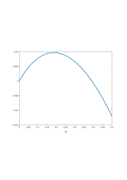
and we choose the following coupling matrix . In Figure 1 on the left we plot the MSF for . The MSF is negative for and remains negative. If we couple the agents via symmetric diffusive coupling as in Example 3, then, in order to synchronize the network we must impose with constant coupling strength. We then need large values of the coupling strength, namely for agents and for . We instead employ our technique and consider an asymmetric tridiagonal coupling. Of course, as we will see in our numerical experiments, the lack of symmetry causes a large transient and the basin of attraction of the synchronous periodic orbit is in general affected by it, see [11] for more details on this.
We have some freedom on what values we select for the
eigenvalues of . We experimented with many different
choices for these values and below we report on two different experiments:
i) select the eigenvalues linearly spaced in , and
ii) take the eigenvalues to be Chebyshev points of the first kind (rescaled
to or to larger intervals, as needed).
For and agents we take eigenvalues in the interval .
In both cases, all the elements of the coupling matrix are less than . We take an initial condition on the attractor and perturb it with a normally distributed perturbation vector. Then we integrate the network with a 4-th order Runge Kutta method and fixed stepsize . For these methods, theoretical results insure that for sufficiently small the numerical method has a closed invariant curve. The distance of this curve from the synchronous periodic orbit is an (see [4]).
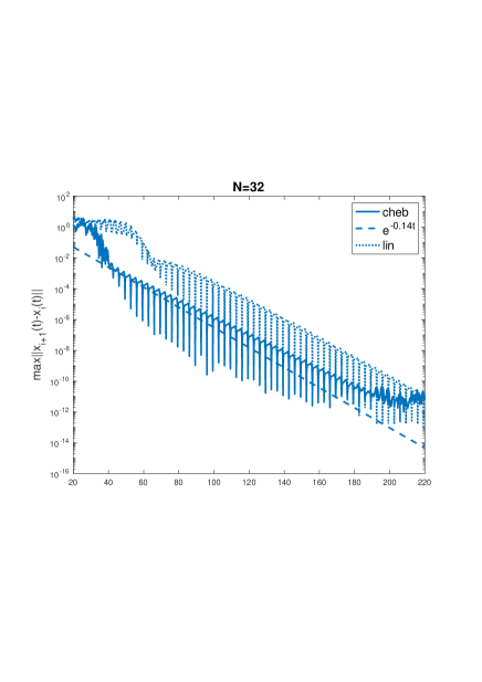
We synchronize agents with both choices of eigenvalues. To witness, in Figure 1 on the right we plot at the grid points. The greatest value of the MSF is obtained for , and it is . We plot as well in order to appreciate the convergence speed to the synchronous solution. The plots are obtained for one initial condition, but the behavior we observe is consistent for every normally distributed random perturbation we considered. The transient in this case is relatively short.
For and linearly spaced eigenvalues the convergence speed remains the same but we do not seem to reach synchronization up to the order of the method. The right plot in Figure 2 is obtained for stepsize , but the behavior is the same also for greater and smaller stepsizes. With Chebyshev points the distance between agents reaches an and does not decrease to machine precision, see the dotted line in the left plot of Figure 2, labeled as “Tridiagonal”.
We also consider an optimal network in the sense of [13], which in the present nearest neighbor topology constrains us to take an outer degree matrix bidiagonal with one eigenvalue at and one eigenvalue with algebraic multiplicity
. Nonetheless, the results obtained for the MSF are still valid, see [13] for details.222To give an intuition of why the MSF theory still works in this case, it suffices to consider the linear system , with coefficient matrix given by a unique Jordan block with eigenvalue . For these kind of systems, the norm of the general solution, after a transient growth, converges to 0. This said, we expect the general solution of , to have a long transient. This is caused by the presence of terms equal to , with , in the explicit expression of the general solution. This long transient affects the behavior of the network as well. Beware that with this choice the dynamics of the last agent does not depend on the other agents. For our experiments we choose two different values of : and . For both values of , the MSF is and hence we expect synchronization with convergence speed .
We represent the norm of the corresponding solutions in the left plot of Figure 2 with a solid line. For we clearly see the expected convergence speed, but not for .
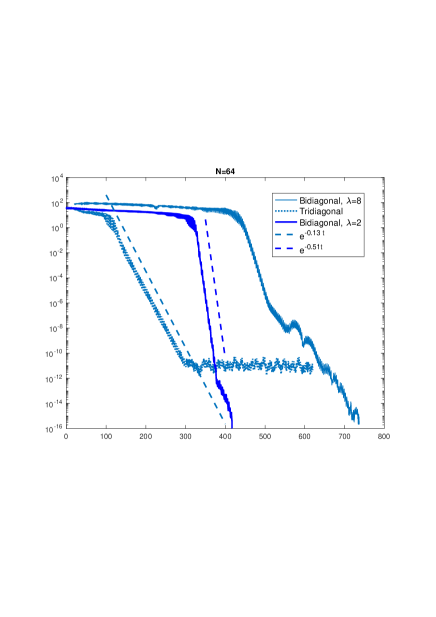
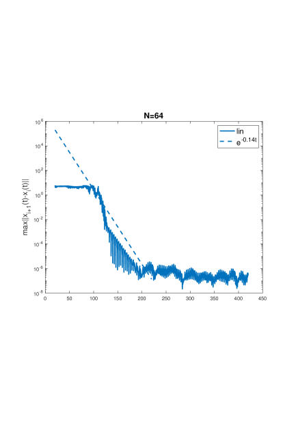
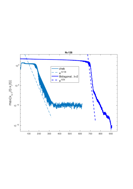
We can synchronize also agents with eigenvalues equal to Chebyshev points of the first kind, but we need to rescale them to the larger interval . For this interval choice, the elements of the coupling matrix are all smaller than . Recall that if we use diffusive coupling and constant coupling strength we need instead . We plot
in Figure 3. If instead we choose the Chebyshev points rescaled in , after a transient, the norm is and it does not seem to decrease any further. As for the case of agents, also in this case of agents we considered the behavior of a bidiagonal network with ; as reported in Figure 3, there is a long transient after which synchronization occurs at the expected convergence rate of .
For and linearly spaced eigenvalues instead, the numerical solution converges toward a non synchronous attractor.
3.2. Rössler
Next, we consider a network of identical Rössler oscillators. Each agent satisfies the system
| (11) |
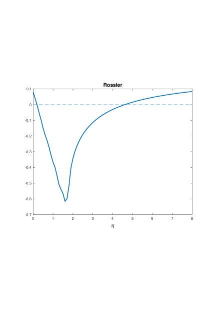
and we choose the coupling matrix in (6) given by . In Figure 4, on the left, we plot the MSF in function of . The MSF is negative in the interval .
If we use diffusive coupling with a constant coupling strength , like in Example 3, then (see the explicit values of the eigenvalues given in Example 3), in order to synchronize agents, we need and . A necessary condition for agents to synchronize is then and as soon as this condition is not satisfied and hence we cannot hope to synchronize more than agents with diffusive coupling and constant coupling strength. In [14] the authors use diffusive coupling in a circular array and can synchronize up to agents, but already with agents the necessary conditions for synchronization are not met anymore.333The authors of [14] point our that, with symmetric tridiagonal Laplacians there will always be an upper limit in the size of a the network in order to obtain a stable synchronous chaotic orbit. With our technique, in principle there is not such limitation.
In what follows we couple and synchronize a network of 64 Rössler agents with our technique, about the chaotic orbit of a single Rössler oscillator.
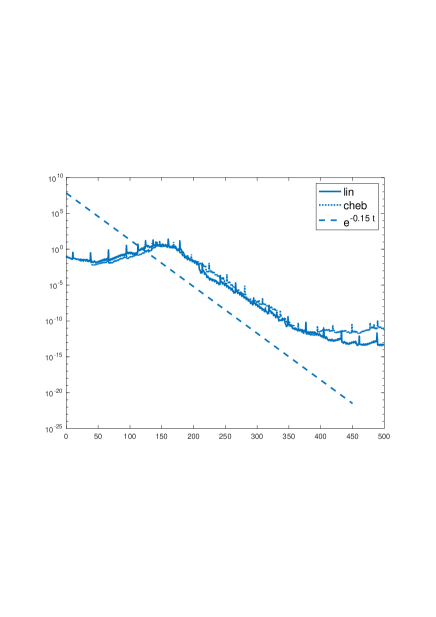
We report on experiments with two different sets of eigenvalues: linearly spaced in , and Chebyshev points of the first kind (rescaled to ). We consider initial conditions obtained by adding a normally distributed perturbation with variance of a synchronous initial condition and integrate (6) to verify that indeed we obtain synchronization. In Figure 4 we plot for the two choices of eigenvalues. For , the corresponding value of the MSF is and the dashed line in the right plot is the graph of . It is clear that, after a transient, the convergence speed of the two perturbed solutions is also . For oscillators, after a longer transient, the quantity is not monotone and oscillates between and .
References
- [1] M. Chu and G.H. Golub. Structured inverse eigenvalue problems. Acta Numerica, pp. 1-71, 2002.
- [2] M. Chu and G.H. Golub. Inverse Eigenvalue Problems. Oxford Science Publications. Oxford University Press, New York, 2013.
- [3] L. Dieci and A. Pugliese. Forming a symmetric, unreduced, tridiagonal matrix with a given spectrum. arXiv preprint 2311.02677, 2023.
- [4] T. Eirola. Invariant curves of one-step methods. BIT, 28-1, pp. 113-122 (1988).
- [5] L.H. Golub and C.F. Van Loan. Matrix Computations. Johns Hopkins Studies in the Mathematical Sciences. Johns Hopkins University Press, 2013.
- [6] J. Hale. Diffusive Coupling, Dissipation, and Synchronization. Journal of Dynamics and Differential Equations, 9-1, pp. 1-52 (1997).
- [7] R. Horn and C. Johnson. Matrix Analysis, 2nd Edition. Cambridge Univ Press 2013.
- [8] L. Huang, Q. Chen, Y-C Lai and L.M. Pecora. Generic behavior of master-stability functions in coupled nonlinear dynamical systems. Physical Review E, 80, 036204-1-11 (2009).
- [9] L.G. Molinari. Lesson 6: Tridiagonal Matrices. https://api.semanticscholar.org/CorpusID:232239257, 2019.
- [10] A.E. Motter, C. Zhou and J. Kurths Enhancing complex-network synchronization. Europhysics Letters, vol. 69, n. 3, (2005).
- [11] R. Muolo, T. Carletti, J.P. Gleeson and M. Asllani Synchronization Dynamics in Non-Normal Networks. Entropy 2021, 23, 36
- [12] T. Muir. Treatise on the Theory of Determinants. Revised and Enlarged by William H. Metzler. New York: Dover Publications 1960.
- [13] T. Nishikawa and A.E. Motter Maximum performance at minimum cost in network synchronization. Physica D, vol. 224, (2006).
- [14] L. Pecora and T. Carroll. Master Stability Functions for Synchronized Coupled Systems. Physical Review Letters, vol. 80, n. 10, (1997), pp. 2109-1112.
- [15] G. Schmeisser. A real symmetric tridiagonal matrix with a given characteristic polynomial. Linear Algebra Appl.s, 193, pp. 11-18 (1993).
- [16] J.J.P. Veerman and R. Lyons. A primer on Laplacian dynamics in directed graphs, Nonlinear Phenomena in Complex Systems, 2020, url=https://api.semanticscholar.org/CorpusID:211066395.