Determining Modes, Synchronization, and Intertwinement

Abstract.

This article studies the interrelation between the determining modes property in the two-dimensional (2D) Navier-Stokes equations (NSE) of incompressible fluids and the synchronization property of two filtering algorithms for continuous data assimilation applied to the 2D NSE. These two properties are realized as manifestations of a more general phenomenon of self-synchronous intertwinement. It is shown that this concept is a logically stronger form of asymptotic enslavement, as characterized by the existence of finitely many determining modes in the 2D NSE. In particular, this stronger form is shown to imply convergence of the synchronization filter and the nudging filter from continuous data assimilation (CDA), and then subsequently invoked to show that convergence in these filters implies that the 2D NSE possesses finitely many determining modes. The main achievement of this article is to therefore identify a new concept, that of self-synchronous intertwinement, through which a rigorous relationship between the determining modes property and synchronization in these CDA filters is established and made decisively clear. The theoretical results are then complemented by numerical experiments that confirm the conclusions of the theorems.

Keywords: determining modes, synchronization, continuous data assimilation, synchronization filter, nudging filter, coupling, Navier-Stokes equations
MSC 2010 Classifications: 35Q30, 35B30, 37L15, 76B75, 76D05, 93B52

1. Introduction

In a seminal paper by C. Foias and G. Prodi [FP67], it was shown that the two-dimensional (2D) externally forced, Navier-Stokes equations (NSE) for incompressible fluids, given by the system

$$\partial_{t}u+u\cdotp\nabla u=-\nabla p+\nu\Delta u+f,\quad\nabla\cdotp u=0,$$ (1.1)

asymptotically possesses a large, but finite number of degrees of freedom, a property that is expected to hold true for turbulent flows on the basis of physical principles. In particular, they introduce the notion of determining modes and subsequently show that the 2D NSE possesess finitely many such modes. This notion characterizes the property that knowledge of the asymptotic behavior of a distinguished set of constitutive modes of the solution suffice to describe the asymptotic behavior of all of its modes. In this way, one therefore captures the finite-dimensionality of the dynamics of the system. It is remarkable that this fact was established at the advent of the study of chaotic dynamical systems, just a few years after E. Lorenz introduced his three-mode truncation of the Boussinesq approximation of the full Navier-Stokes equations for weather prediction [Lor63]. It had also provided strong evidence for the finite dimensionality of the global attractor of the 2D incompressible NSE, which was eventually resolved in the two decades following [FP67] in [FT79, Lad85, CFT88].

This result has since been realized as a fundamental cornerstone in the study of the dynamics of the 2D NSE and many other dissipative partial differential equations (PDEs), deterministic and stochastic. It has since either motivated or found intimate connection to estimates on dissipative length scales of turbulent flows [FMTT83, FT87, CFMT85], the study of dimension-reduction, approximate inertial manifolds, and downscaling in dissipative systems [FT91, OT03, AOT14, KKZ23], and the existence of determining forms [FJKT12, FDKT14, JST15, JST17, FJLT17, JMST18], a notion weaker than that of an inertial form, in which the dynamics of the underlying PDE system is reduced to the study a bona fide ODE system, albeit an infinite-dimensional one. Determining modes have also found a wide range of applications in the domains of data assimilation [BLSZ13], numerical approximation of PDEs [MT18, IMT19], parameter estimation [CHL20, CHL⁺22, PWM22, Mar22, BH23, Mar24, FLMW24, AB24], and perhaps most notably, the problem of unique ergodicity for stochastically forced systems [EMS01, KS12, Deb13], where it is often referred to as the Foias-Prodi property. In the context of the 2D NSE, the concept of determining modes has also been extended to accommodate the concepts of determining nodes, volume elements, and, more generally, determining functionals [FT84, CJT97, JT92b, JT92a, CDS03], which have all enjoyed a richness in application [FL99, Lan03, HOT11, FJT15, ANLT16, FMT16, JMT17, ATG⁺17, FJJT18, DLMB18, CDLMB18, OBK18, BFMT19, ZRSI19, IMT19, LRZ19, COT19, GAN20, BBJ21, CO23, YGJP22, HTHK22, JP23, GALNR24, KEML⁺24].

In some of these applications, the existence of finitely many determining modes is not invoked explicitly, but rather appears implicitly through the analysis. Although it is by now well-known how the Foias-Prodi mechanism appears in these applications, as of yet, there has been no result that explicitly relates the Foias-Prodi property of the Navier-Stokes equations to the particular application in which its mechanism appears. Indeed, in the context of either data assimilation or unique ergodicity, the existence of such a relation is inferred through either how closely the analysis matches that carried out in [FP67], or in anticipating how solutions should behave as a consequence of the property, thereby informing the approach that is developed for the application itself. For example, in proving that the continuous data assimilation algorithms of E. Olson and E. Titi [OT03] or A. Azouani, E. Olson, and E. Titi [AOT14] are capable of asymptotically recovering the reference state variable from partial observations of the system, i.e., achieving synchronization of the data assimilated approximating state variable with the reference state variable, one observes strong similarities to the argument of C. Foias and G. Prodi in [FP67]. However, whether or not one property implies the other is not known. In the context of unique ergodicity of degenerate stochastically forced systems, asymptotic couplings or exact finite-dimensional couplings have been constructed to deduce uniqueness of invariant probability measures for its Markovian dynamics, and even deduce mixing rates. Due to the degeneracy of the noise, the design of these couplings are restricted to enforcing a form of contractivity only on a finite, but potentially large, dimensional subspace. However, for systems possessing the Foias-Prodi property, contractivity on a finite-dimensional subspace subsequently activates a nonlinear deterministic mechanism that enforces contractivity on the complementary space. Couplings are then designed by incorporating system controls in such a way that exploit this intrinsic property in a convenient way [DO05, Oda06, HM06, KS00, Shi08, HMS11, GHMR17, BKS20, GHMR21, GHMN22, FZ23, CBK23, BFZ23, Ngu23].

In this article, we establish a precise and rigorous relation between the existence of finitely many determining modes and the ability of the Olson-Titi (OT) and Azouani-Olson-Titi (AOT) continuous data assimilation (CDA) algorithms to converge in the paradigmatic context of the 2D Navier-Stokes system, the latter of which implements a control that has been fruitfully exploited in studying the problem of unique ergodicity for stochastically forced systems [GHMR17, BKS20, GHMR21, FZ23, BFZ23, Ngu23]. These data assimilation algorithms are closely related to couplings that have been designed in the study of the problem of unique ergodicity for many stochastically-driven equations in hydrodynamics. Motivated by the stochastic-control ideas developed in the design of couplings, we establish this relation by introducing a new, but closely related concept of intertwinement, and show that in fact a stronger property holds, which is the existence of what we call self-synchronous intertwinements. From this property, one can deduce both the finite determining modes property and synchronization property of two particular data assimilation algorithms as direct consequences. By doing so, we develop an expanded theory in which determining modes and synchronization of continuous data assimilation can be studied simultaneously. Due to the close relation of these CDA algorithms to the couplings that have been constructed in the literature, it is our hope that these ideas will also eventually find application in the study of stochastically forced systems.

In the remainder of the introduction, we hold an informal discussion of the central ideas, deferring their rigorous statements for later on.

1.1. Intertwinements: The Heart of the Matter

The primary motivation of this paper is to establish a direct connection between the existence of determining modes for the 2D NSE and the convergence of two particular filtering algorithms for continuous data assimilation. As previously mentioned, it is a folklore that the two are intimately related due to the similarity in the proofs of these respective properties. Nevertheless, answers to basic questions regarding whether one property implies the other have hitherto been unaddressed. This paper is an attempt to give clarity to this issue.

The two algorithms of interest are the synchronization filter and the nudging filter. Consider a solution $u$ to (1.1). Let $p=P_{N}u$ and $Qu=Q_{N}u$, where $Q_{N}=I-P_{N}$. Given $N>0$, the synchronization filter is defined as the function $v$, which satisfies:

$$\begin{split}v&=p+q,\\ \partial_{t}q+Q_{N}[(p+q)\cdotp\nabla(p+q)]&=-Q_{N}\nabla r+\nu\Delta q+Q_{N}f,\quad\nabla\cdotp q=0,\quad q(0)=q_{0},\end{split}$$ (1.2)

where $q_{0}$ does not necessarily equal $Qu_{0}$. On the other hand, the nudging filter is defined as the function $\tilde{v}$, which satisfies

$$\partial_{t}\tilde{v}+(\tilde{v}\cdotp\nabla)\tilde{v}=-\nabla\tilde{r}+\nu\Delta\tilde{v}+f-\mu P_{N}\tilde{v}+\mu P_{N}u,\quad\nabla\cdotp\tilde{v}=0,\quad\tilde{v}(0)=\tilde{v}_{0},$$ (1.3)

where $\tilde{v}_{0}$ does not necessarily satisfy $P_{N}\tilde{v}_{0}=p_{0}$, and may be taken to be arbitrary. In (1.2) and (1.3) are proposed as solutions to the problem of recovering the unobserved component, $Qu$, of the underlying 2D NSE system. “Convergence” of these algorithms refer to the property that $v$ and $\tilde{v}$ synchronize with $u$. Informally, this means that there exist appropriate choices of $N$ and $\mu$ such that

$$\lim_{t\rightarrow\infty}|v(t)-u(t)|=\lim_{t\rightarrow\infty}|\tilde{v}(t)-u(t)|=0.$$ (1.4)

Morally speaking, synchronization of (1.2) and (1.3) with (1.1) is a concrete manifestation of the determining modes property since it not only asserts that knowledge of a sufficiently many modes, $p$, is enough to asymptotically determine the unobserved modes, $Qu$, but moreover furnishes an explicit approximation of the unobserved modes, $q\approx Qu\approx Q_{N}\tilde{v}$. It is therefore natural to expect that this synchronization property is directly relatable to the existence of finitely many determining modes for (1.1).

Suppose that either one of the algorithms above possesses the synchronization property (1.4). To show that this property implies that (1.1) has the determining modes property, i.e., has finitely many determining modes, one must establish, for any pair of solutions $u_{1},u_{2}$ corresponding to external forces $f_{1},f_{2}$, the existence of a cut-off, $N$, with the following property:

$$\lim_{t\rightarrow\infty}|P_{N}u_{1}(t)-P_{N}u_{2}(t)|=\lim_{t\rightarrow\infty}|f_{1}(t)-f_{2}(t)|=0\quad\text{implies}\quad\lim_{t\rightarrow\infty}|u_{1}(t)-u_{2}(t)|=0.$$ (1.5)

Let $(v_{1},v_{2})$ be a pair satisfying either (1.2) or (1.3) respectively corresponding to forces $(f_{1},f_{2})$. Then, by assumption, for $N$ sufficiently large, $v_{j}$ synchronizes with $u_{j}$. By the triangle inequality, one has

$$|u_{1}-u_{2}|\leq|u_{1}-v_{1}|+|v_{1}-v_{2}|+|v_{2}-u_{2}|,$$ (1.6)

so that by the synchronization property, one obtains

$$\lim_{t\rightarrow\infty}|u_{1}(t)-u_{2}(t)| \leq\limsup_{t\rightarrow\infty}|v_{1}(t)-v_{2}(t)|.$$

On the other hand

$$|P_{N}v_{1}-P_{N}v_{2}|\leq|P_{N}v_{1}-P_{N}u_{1}|+|P_{N}u_{1}-P_{N}u_{2}|+|P_{N}u_{2}-P_{N}v_{2}|,$$ (1.7)

Then by a second application of the synchronization property, which guarantees $|P_{N}v_{j}-P_{N}u_{j}|\rightarrow 0$, in addition to the determining modes hypothesis (1.5), namely that $|P_{N}u_{1}-P_{N}u_{2}|\rightarrow 0$, one deduces from (1.7) that

$$\lim_{t\rightarrow\infty}|P_{N}v_{1}(t)-P_{N}v_{2}(t)|=0.$$

Therefore, if one can guarantee that (1.2) or (1.3) themselves possesses a determining modes-type property that allows one to deduce that $|v_{1}(t)-v(t)|\rightarrow 0$ as $t\rightarrow\infty$ from the fact that $|P_{N}v_{1}(t)-P_{N}v_{2}(t)|\rightarrow 0$, as $t\rightarrow\infty$, then one may conclude from the argument above that $|u_{1}(t)-u_{2}(t)|\rightarrow 0$.

A natural temptation is to attempt to deduce the determining modes property of (1.2) or (1.3) as a consequence of the determining modes property for (1.1) by a careful selection of $f_{1},f_{2}$. While this indeed is the main mechanism at play, it is not rigorously possible to do so since the choice one must make requires $f_{1},f_{2}$ to be state-dependent. For instance, one may view a pair of solutions $(\tilde{v}_{1},\tilde{v}_{2})$ to (1.3) corresponding to forces $(\tilde{f}_{1},\tilde{f}_{2})$, as a pair of solutions to (1.1) corresponding to forces $(f_{1},f_{2})=(\tilde{f}_{1}-\mu P_{N}\tilde{v}_{1}+\mu P_{N}u_{1},\tilde{f}_{2}-\mu P_{N}\tilde{v}_{2}+\mu P_{N}u_{2})$. Thus, $f_{j}=f_{j}(\tilde{v}_{j})$ and the equation is, strictly speaking, no longer the same equation as (1.1), but is rather a perturbation of the (1.1). The obstruction is now clear and the problem reduces to addressing the following question: What class of perturbations to (1.1) allow one to formulate and establish a determining modes-type property? This is purpose of the concept of intertwinement.

The key idea is to view the determining modes property of (1.1) as a property of the augmented system in which the pair $(u_{1},u_{2})$ simultaneously satisfies (1.1) corresponding to forcing $(f_{1},f_{2})$, respectively:

$$\begin{split}\partial_{t}u_{1}+(u_{1}\cdotp\nabla)u_{1}&=-\nabla p_{1}+\nu\Delta u_{1}+f_{1},\quad\nabla\cdotp u_{1}=0\\ \partial_{t}u_{2}+(u_{2}\cdotp\nabla)u_{2}&=-\nabla p_{2}+\nu\Delta u_{2}+f_{2},\quad\nabla\cdotp u_{2}=0.\end{split}$$ (1.8)

In the context of stochastic forcing, $f\sim dW$, such an augmented system is at once recognized as the independent coupling. On the other hand, (1.2) can be viewed as a coupled system in $(u,v)$ via:

$$\begin{split}\partial_{t}u+(u\cdotp\nabla)u&=-\nabla p+\nu\Delta u+f,\quad\hskip 108.5pt\nabla\cdotp u=0\\ \partial_{t}v+(v\cdotp\nabla)v&=-\nabla q+\nu\Delta v+f+P_{N}((v\cdotp\nabla)v-(u\cdotp\nabla)u),\quad\nabla\cdotp v=0.\end{split}$$ (1.9)

In the context of stochastic forcing, (1.9) is analogous to an exact coupling on a finite-dimensional subspace, since the control term, $P_{N}((v\cdotp\nabla)v-(u\cdotp\nabla)u)$ serves to enforce $P_{N}v=P_{N}u$ exactly. Lastly, (1.3) can also be viewed as a coupled system in $(u,\tilde{v})$ as:

$$\begin{split}\partial_{t}u+(u\cdotp\nabla)u&=-\nabla p+\nu\Delta u+f,\quad\hskip 74.5pt\nabla\cdotp u=0\\ \partial_{t}\tilde{v}+(\tilde{v}\cdotp\nabla)\tilde{v}&=-\nabla q+\nu\Delta\tilde{v}+f-\mu P_{N}\tilde{v}+\mu P_{N}u,\quad\nabla\cdotp v=0.\end{split}$$ (1.10)

In the context of stochastic forcing, the term $f-P_{N}v+P_{N}u$ may often be viewed as a Girsanov shift of underlying stochastic forcing $f$, and (1.10) has been exploited as an asymptotic coupling.

Now, upon taking two copies, $(\tilde{v}_{1},\tilde{v}_{2})$, of the second component of (1.10), and two copies, $(v_{1},v_{2})$, of the second component of (1.9), respectively corresponding to the pair of forces $(f_{1},f_{2})$, one has:

$$\begin{split}\partial_{t}\tilde{v}_{1}+(\tilde{v}_{1}\cdotp\nabla)\tilde{v}_{1}&=-\nabla\tilde{q}_{1}+\nu\Delta\tilde{v}_{1}+\tilde{f}_{1}-\mu P_{N}\tilde{v}_{1},\quad\nabla\cdotp\tilde{v}_{1}=0,\\ \partial_{t}\tilde{v}_{2}+(\tilde{v}_{2}\cdotp\nabla)\tilde{v}_{2}&=-\nabla q_{2}+\nu\Delta\tilde{v}_{2}+\tilde{f}_{2}-\mu P_{N}\tilde{v}_{2},\quad\nabla\cdotp\tilde{v}_{2}=0,\end{split}$$ (1.11)

where $\tilde{f}_{1}=f_{j}+\mu P_{N}u_{j}$, and

$$\begin{split}\partial_{t}v_{1}+(v_{1}\cdotp\nabla)v_{1}&=-\nabla q_{1}+\nu\Delta v_{1}+\tilde{f}_{1}+P_{N}(v_{1}\cdotp\nabla)v_{1},\quad\nabla\cdotp v_{1}=0.\\ \partial_{t}v_{2}+(v_{2}\cdotp\nabla)v_{2}&=-\nabla q_{2}+\nu\Delta v_{2}+\tilde{f}_{2}+P_{N}(v_{2}\cdotp\nabla)v_{2},\quad\nabla\cdotp v_{2}=0,\end{split}$$ (1.12)

where $\tilde{f}_{j}=f_{j}-P_{N}(u_{j}\cdotp\nabla)u_{j}$.

In each of the above cases, a common structure is readily identified:

$$\partial_{t}U+AU+B(U) =f+MF(U),\quad$$ (1.13)

for some $M\in\mathbb{R}^{2\times 2}$, where $U=(u_{1},u_{2})$, $f=(f_{1},f_{2})$, and $F(U)=(F(u_{1}),F(u_{2}))$. We refer to (1.13) as an intertwinement of (1.1). In this paper, we formulate a definition similar to the determining modes property, but in the generality of (1.13) (see 3.0.2, 3.0.4). We then identify several examples of $M$ and $F$ in which one can directly verify that (1.13) satisfies this generalized determining modes-type property, thereby demonstrating the fruitfulness of our definition. In a word, 3.0.4 is a sublimation of the concept of the determining modes property, originally formulated for a given system, into a property formulated for a lifting of the system (into a product space), which is induced by coupling the system to itself in a particular way, i.e., the intertwined system. In the lifted space, the determining modes property becomes a property about the lifted system’s ability to self-synchronize. These ideas are formally introduced in Section 3, along with several examples. The main results regarding how intertwinement, determining modes, and the synchronization and nudging filters of continuous data asssimlation are related are developed in Section 4. The proofs of the main results are presented in Section 5. Before proceeding to these sections, we provide the relevant mathematical preliminaries in Section 2. Finally, conclude the paper in Section 6 with a series of computational results that corroborate the theoretical results.

2. Mathematical Preliminaries

We let $H$ denote the space of $L^{2}$ real-valued vector fields, which are $2\pi$-periodic in each direction, divergence-free, and mean-free over $\Omega$, in the sense of distribution. We let $\mathbb{P}$ denote the Leray projection. Observe that $\mathbb{P}H=H$. We let $V$ denote the subspace of $H$ endowed with the $V$ topology. We make use of the following notation for the inner products and norms on $H$ and $V$, respectively:

$$\left(u,v\right)=\int_{\Omega}u(x)\cdotp v(x)dx,\quad|u|^{2}=\left(u,u\right),$$ (2.1)

and

$$((u,v))=\sum_{j=1,2}\int_{\Omega}\partial_{j}u(x)\cdotp\partial_{j}v(x)\ dx,\quad\lVert u\rVert^{2}=((u,u)).$$ (2.2)

The dual spaces of $H,V$ will be denoted by $H^{*},V^{*}$ respectively. Then we have the following continuous imbeddings

$$V\subset H\subset H^{*}\subset V^{*}.$$

In particular, we have the Poincaré inequality

$$|u|\leq\lVert u\rVert,$$ (2.3)

for all $u\in V$. For each $1\leq p\leq\infty$, we will also make use of the Lebesgue spaces, $L^{p}$, which denote the space of $p$-integrable functions endowed with the following norm:

$$\lvert u\rvert_{p}=\left(\int_{\Omega}|u(x)|^{p}dx\right)^{1/p},$$ (2.4)

with the usual modification when $p=\infty$. For convenience, we will view them as subspaces of completely integrable functions over $\Omega$, which are mean-free and $2\pi$-periodic in each direction. It will be convenient to abuse notaiton and consider $L^{p}$ as a space of either scalar functions or vector fields. In this way, we have $H\subset L^{2}$, and $L^{p}\subset H$.

Lastly, we denote the Stokes operator by $A=-\mathbb{P}\Delta$ and define, for each $n\geq 0$, integer powers, $A^{n/2}$, of $A$ by

$$A^{n/2}u=\sum_{k\in\mathbb{Z}^{2}\setminus\{(0,0)\}}\hat{u}_{k}w_{k},\quad w_{k}(x)=\cos(k\cdotp x).$$ (2.5)

Then the domain, $D(A^{n/2})$, of $A^{n/2}$ is a subspace of $H$ endowed with the topology induced by

$$\lVert u\rVert_{n}=|A^{n/2}u|=\left(\sum_{k\in\mathbb{Z}^{2}}|k|^{2n}|\hat{u}_{k}|^{2}\right)^{1/2}.$$ (2.6)

Observe that

$$|u|=\lvert u\rvert_{0},\qquad\rVert u\rVert=\lVert u\rVert_{0}=\lvert A^{1/2}u\rvert_{0}.$$

Our analysis will make use of the Ladyzhenska and Agmon, respectively, interpolation inequalities: there exist absolute constants $C_{L},C_{A}>0$ such that

$$\lvert u\rvert_{4}^{2}\leq C_{L}\lVert u\rVert|u|,\qquad\lvert u\rvert_{\infty}^{2}\leq C_{A}|Au||u|.$$ (2.7)

Another useful interpolation inequality, is the following:

$$\lVert u\rVert^{2}\leq|Au||u|$$ (2.8)

We will also make use of the Bernstein inequality: let $P_{N}$ denote projection onto Fourier wavenumbers, $|k|\leq N$, where $N>0$ is a real number. Denote the complementary projection by

$$Q_{N}\mathrel{\mathop{\mathchar 58\relax}}=I-P_{N}$$ (2.9)

Then for any integers $m\leq n$

$$\lVert P_{N}u\rVert_{n}\leq N^{n-m}\lVert P_{N}u\rVert_{m},\quad\lVert Q_{N}u\rVert_{m}\leq N^{m-n}\lVert Q_{N}u\rVert_{n}.$$ (2.10)

Observe that we also have the following borderline Sobolev inequality

$$|P_{N}u|_{\infty}\leq C_{S}(\ln N)^{1/2}\|P_{N}u\|$$ (2.11)

Given $f\in L^{\infty}(0,\infty;H)$, the generalized Grashof number is defined as

$$\mathfrak{G}\mathrel{\mathop{\mathchar 58\relax}}=\frac{\sup_{t\geq 0}|f(t)|}{\nu^{2}}.$$ (2.12)

If $f\in L^{\infty}(0,\infty;D(A^{n/2}))$, then for each integer $n\geq 1$, we define the shape factors of $f$ by

$$\sigma_{n}\mathrel{\mathop{\mathchar 58\relax}}=\frac{\sup_{t\geq 0}|A^{n/2}f(t)|}{|f|}.$$ (2.13)

We will rewrite (1.1) in its functional form:

$$\frac{du}{dt}+\nu Au+B(u,u)=f,\quad u(0)=u_{0},$$ (2.14)

where

$$B(u,v)\mathrel{\mathop{\mathchar 58\relax}}=\mathbb{P}((u\cdotp\nabla)v).$$ (2.15)

We also have the well-known, skew-symmetric property of $\left(B(u,v),w\right)$:

$$\left(B(u,v),w\right)=-\left(B(u,w),v\right),$$ (2.16)

for $u,v,w\in V$, which immediately implies

$$\left(B(u,v),v\right)=0.$$

We will also make use of the identity

$$\left(B(u,u),Au\right)=0.$$ (2.17)

Observe that $B\mathrel{\mathop{\mathchar 58\relax}}D(A)\times V\rightarrow H$ via

$$|B(u,v)|\leq C_{A}^{1/2}|Au|^{1/2}|u|^{1/2}\|v\|.$$ (2.18)

whenever $u\in D(A)$ and $v\in V$. Moreover, $B$ is also continuous as a bilinear mapping $B\mathrel{\mathop{\mathchar 58\relax}}V\times V\rightarrow V^{\prime}$ via

$$|\left(B(u,v),w\right)|\leq C_{L}\lVert u\rVert^{1/2}|u|^{1/2}\lVert v\rVert\|w\|^{1/2}|w|^{1/2},$$ (2.19)

where $u,v\in V$ and $w\in V$, and $C_{L}$ is the constant appearing in (2.7). The Frechét derivative of $B$ will be denoted by $DB$. Recall that $DB$ is defined by

$$DB(u)v=B(u,v)+B(v,u).$$ (2.20)

By (2.18), it follows that $DB\mathrel{\mathop{\mathchar 58\relax}}D(A)\rightarrow L(D(A),H)$, $u\mapsto DB(u)$, while (2.19) implies $DB\mathrel{\mathop{\mathchar 58\relax}}V\rightarrow L(V,V^{\prime})$, where $L(X,Y)$ denotes the space of bounded linear operators mapping $X$ to $Y$.

We recall the following classical global existence and uniqueness result.

Theorem 2.0.1.

Let $f\in L^{\infty}(0,\infty;H)$. Then for each $u_{0}\in V$ and $T>0$, there exists a unique solution $u\in C([0,T];V)\cap L^{2}(0,T;D(A))$ such that $u(0)=u_{0}$. Moreover, there exists $t_{0}=t_{0}(\|u_{0}\|,|f|)$ such that

$$\sup_{t\geq t_{0}}|u(t)|\leq\nu\sigma_{-1}\mathfrak{G}=\mathrel{\mathop{\mathchar 58\relax}}\rho_{0},\qquad\sup_{t\geq t_{0}}\|u(t)\|\leq\nu\mathfrak{G}=\mathrel{\mathop{\mathchar 58\relax}}\rho_{1}.$$ (2.21)

In fact, the balls $B_{H}(\rho_{0})$ and $B_{V}(\rho_{1})$ are forward-invariant sets for (2.14)

We will refer to the solutions guaranteed by 2.0.1 as strong solutions. We note that the forward-invariance of $B_{H}(\rho_{0})$ and $B_{V}(\rho_{1})$ follow from the elementary inequalities which hold for strong solutions of (2.14):

$$\begin{split}|u(t)|^{2}&\leq e^{-\nu t}|u_{0}|^{2}+\rho_{0}^{2}(1-e^{-\nu t}),\\ \lVert u(t)\rVert^{2}&\leq e^{-\nu t}\lVert u_{0}\rVert^{2}+\rho_{1}^{2}(1-e^{-\nu t}),\end{split}$$ (2.22)

for all $t\geq 0$ and $u_{0}\in V$, and let $p=P_{N}u$ denote the projection of $u$ onto the wave-numbers $|k|\leq N$.

We will also make use of the global well-posedness (in the sense of 3.0.3) of the corresponding initial value problems for synchronization filter and the nudging system, which were developed in [OT03] and [AOT14], respectively. We state them here for the sake of completeness. For both statements, given $f\in L_{loc}^{\infty}(0,\infty;H)$ and $u_{0}\in V$, we let $u$ denote the unique global-in-time solution to (2.14) such that $u\in C([0,T];V)\cap L^{2}(0,T;D(A))$ and $\frac{du}{dt}\in L^{2}(0,T;H)$, for all $T>0$.

Theorem 2.0.2 (Theorem 3.1, [OT03]).

For any $N>0$ and $q_{0}\in V$ such that $Q_{N}q_{0}=q_{0}$, there exists a unique $q$ such that $q\in C([0,T];V)\cap L^{2}(0,T;D(A))$, $\frac{dq}{dt}\in L^{2}(0,T;H)$, for all $T>0$, and satisfies

$$\frac{dq}{dt}+\nu Aq+Q_{N}B(p+q,p+q)=Q_{N}f,\quad q(0)=q_{0}.$$ (2.23)

In particular, for $v=P_{N}u+q$, the pair $(u,v)$ equivalently satisfies the following system of equations:

$$\begin{split}\frac{du}{dt}+\nu Au+B(u,u)&=f,\quad u(0)=u_{0}\\ \frac{dv}{dt}+\nu Av+B(v,v)&=f+P_{N}\left(B(v,v)-B(u,u)\right),\quad v(0)=P_{N}u_{0}+q_{0}.\end{split}$$ (2.24)

Theorem 2.0.3 (Theorem 6, [AOT14]).

For any $N>0$ and $\tilde{v}_{0}\in V$, there exists a unique $\tilde{v}$ such that $\tilde{v}\in C([0,T];V)\cap L^{2}(0,T;D(A))$, $\frac{d\tilde{v}}{dt}\in L^{2}(0,T;H)$, for all $T>0$, and satisfies

$$\frac{d\tilde{v}}{dt}+\nu A\tilde{v}+B(\tilde{v},\tilde{v})=f-\mu P_{N}\tilde{v}+\mu P_{N}u,\quad\tilde{v}(0)=\tilde{v}_{0}.$$ (2.25)

In particular, the pair $(u,\tilde{v})$ satisfies the following system of equations:

$$\begin{split}\frac{du}{dt}+\nu Au+B(u,u)&=f,\quad u(0)=u_{0}\\ \frac{d\tilde{v}}{dt}+\nu A\tilde{v}+B(\tilde{v},\tilde{v})&=f-\mu P_{N}\tilde{v}+\mu P_{N}u,\quad\tilde{v}(0)=\tilde{v}_{0}.\end{split}$$ (2.26)

We conclude this section by include two elementary results, which are crucial to establishing several of the main results of this article. The first result is Grönwall-type lemma that controls the long-time behavior of solutions, while the second collects some important bounds on solutions to the heat equation. Both results are fundamental for establishing that various intertwinements are self-synchronous.

Lemma 2.0.4.

Let $z_{1},z_{2},z_{3}\mathrel{\mathop{\mathchar 58\relax}}(0,\infty)\rightarrow[0,\infty)$ be given such that $\lim_{t\rightarrow\infty}z_{j}(t)=0$, for $j=1,2$. Suppose $x\mathrel{\mathop{\mathchar 58\relax}}[0,\infty)\rightarrow[0,\infty)$ is a differentiable function such that

$$x^{\prime}+\alpha x+\beta y\leq z_{1}+z_{2}x+z_{3}y,$$

holds for for all $t>0$, for some $\alpha,\beta>0$, and some dominating function $y\mathrel{\mathop{\mathchar 58\relax}}[0,\infty)\rightarrow[0,\infty)$, i.e., $x\leq y$. Then $\lim_{t\rightarrow\infty}x(t)=0$.

Proof.

Since $z_{j}(t)\rightarrow 0$ as $t\rightarrow\infty$, for $j=1,2,3$, given $0<\epsilon<1$, there exists $t_{0}>0$ such that $z_{1}(t)\leq(\alpha+\beta)\epsilon(1-\epsilon)$ and $z_{2}(t)\leq\alpha\epsilon$, $z_{3}(t)\leq\beta\epsilon$, for all $t\geq t_{0}$. Then

$$x^{\prime}+\alpha x+\beta y \leq(\alpha+\beta)\epsilon(1-\epsilon)+\alpha\epsilon x+\beta\epsilon y,$$

for all $t\geq t_{0}$. In particular

$$x^{\prime}+\alpha(1-\epsilon)x+\beta(1-\epsilon)y \leq(\alpha+\beta)\epsilon(1-\epsilon).$$

Since $x\leq y$, it follows that

$$x^{\prime}+(\alpha+\beta)(1-\epsilon)x\leq(\alpha+\beta)\epsilon(1-\epsilon).$$

Hence

$$x(t) \leq e^{-(\alpha+\beta)(1-\epsilon)(t-t_{0})}x(t_{0})+\epsilon(1-e^{-(\alpha+\beta)(1-\epsilon)(t-t_{0})})$$

$$=e^{-(\alpha+\beta)(1-\epsilon)(t-t_{0})}(x(t_{0})-\epsilon)+\epsilon.$$

Denote by $a_{+}(t)=\max\{a(t),0\}$. We then choose $t_{1}\geq t_{0}$ such that

$$t_{1}\geq t_{0}+\frac{1}{(\alpha+\beta)(1-\epsilon)}\ln\left(\frac{(x(t_{0})-\epsilon)_{+}}{\epsilon}\right).$$

Thus for all $t\geq t_{1}$

$$x(t)\leq 2\epsilon,$$

as desired. ∎

Lemma 2.0.5.

Given $N>0$, $h\in L^{\infty}(0,\infty;H)$, and $p_{0}\in V$ such that $p_{0}=P_{N}p_{0}$. Let $p$ denote the unique solution of the initial value problem

$$\partial_{t}p+\nu Ap=P_{N}h,\quad p(0)=p_{0}.$$

Then $p=P_{N}p$ and

$$\|p(t)\|^{2}\leq e^{-\nu t}\|p(t_{0})\|^{2}+\nu^{2}\left(\frac{\sup_{t\geq 0}|P_{N}h(t)|}{\nu^{2}}\right)^{2},$$

for all $t\geq 0$ and $N>0$. Moreover

$$\sup_{t\geq t_{0}}\|p(t)\|^{2}\leq 2\nu^{2}\left(\frac{\sup_{t\geq t_{0}^{\prime}}|P_{N}h(t)|}{\nu^{2}}\right)^{2}$$ (2.27)

provided that

$$t_{0}\geq t_{0}^{\prime}+\frac{2}{\nu}\ln\left(\frac{\nu\|p(t_{0}^{\prime})\|}{\sup_{t\geq t_{0}^{\prime}}|P_{N}h(t)|}\right),\quad t_{0}^{\prime}\geq\frac{2}{\nu}\ln\left(\frac{\nu\|p_{0}\|}{\sup_{t\geq 0}|P_{N}h(t)|}\right).$$ (2.28)

In particular, if $\lim_{t\rightarrow\infty}|{P_{N}h}(t)|=0$, then $\lim_{t\rightarrow\infty}\|{p}(t)\|=0$.

Proof.

The claim that $p=P_{N}p$ follows simply by applying $P_{N}$ to the heat equation, observing that $P_{N}A=AP_{N}$, then applying uniqueness of solutions.

Next, recall from (5.14) that the energy balance for $p$ is given by

$$\frac{1}{2}\frac{d}{dt}\|{p}\|^{2}+\nu|A{p}|^{2} =\left({h},{Ap}\right).$$

An application of the Cauchy-Schwarz inequality and Gronwall’s inequality then yields

$$\|p(t)\|^{2}\leq e^{-\nu(t-t^{\prime})}\|p(t^{\prime})\|^{2}+\nu^{2}\left(\frac{\sup_{t\geq t^{\prime}}|P_{N}h(t)|}{\nu^{2}}\right)^{2},$$ (2.29)

for all $t\geq t^{\prime}\geq 0$. In particular

$$\sup_{t\geq t_{0}^{\prime}}\|p(t)\|^{2}\leq 2\nu^{2}\left(\frac{\sup_{t\geq 0}|P_{N}h(t)|}{\nu^{2}}\right)^{2},$$ (2.30)

for $t_{0}^{\prime}$ given by (2.28). Furthermore, (2.30) and (2.29) imply

$$\sup_{t\geq t_{0}}\|p(t)\|^{2}\leq 2\nu^{2}\left(\frac{\sup_{t\geq t_{0}^{\prime}}|P_{N}h(t)|}{\nu^{2}}\right)^{2},$$

for $t_{0}$ given by (2.28). ∎

3. The Paradigm of Intertwinement and Self-Synchronization

We recall the definition of determining modes for the 2D NSE, originally introduced by Foias and Prodi in [FP67].

Definition 3.0.1.

Given $f_{1},f_{2}\in L^{\infty}(0,\infty;H)$, let $u_{1}=u(\cdotp;u_{0}^{1}),u_{2}=u(\cdotp;u_{0}^{2})$ denote the global-in-time unique strong solutions of the initial value problems

$$\begin{split}\frac{du_{1}}{dt}+\nu Au_{1}+B(u_{1},u_{1})&=f_{1},\quad u_{1}(0)=u_{0}^{1},\\ \frac{du_{2}}{dt}+\nu Au_{2}+B(u_{2},u_{2})&=f_{2},\quad u_{2}(0)=u_{0}^{2}.\end{split}$$ (3.1)

We say that (2.14) has the finite determining modes property if there exists $N>0$ such that

$$|P_{N}u(t;u_{0}^{1})-P_{N}u(t;u_{0}^{2})|\rightarrow 0\quad\text{and}\quad|f_{1}(t)-f_{2}(t)|\rightarrow 0,\quad\text{as}\ t\rightarrow\infty,$$ (3.2)

implies

$$|u(t;u_{0}^{1})-u(t;u_{0}^{2})|\rightarrow 0,\quad\text{as}\ t\rightarrow\infty,$$ (3.3)

for all $u_{0}^{1},u_{0}^{2}\in V$. The smallest such number $N$ is the number of determining modes.

The thrust of this section is to expand 3.0.1 in a way that effectively allows $f_{1},f_{2}$ to depend on $u_{2},u_{1}$. We do so by introducing the notion of intertwinement.

Definition 3.0.2.

Let $g_{1},g_{2}\in L^{\infty}(0,\infty;H)$ and $F_{1},F_{2}\mathrel{\mathop{\mathchar 58\relax}}V\rightarrow H$ such that $(F_{1}(0),F_{2}(0))=(0,0)$. Then the intertwined Navier-Stokes system is given by

$$\begin{split}\frac{dv_{1}}{dt}+\nu Av_{1}+B(v_{1},v_{1})&=g_{1}+m_{11}F_{1}(v_{1})+m_{12}F_{2}(v_{2})\\ \frac{dv_{2}}{dt}+\nu Au_{2}+B(v_{2},v_{2})&=g_{2}+m_{21}F_{1}(v_{1})+m_{22}F_{2}(v_{2}),\end{split}$$ (3.4)

for some $(m_{ij})_{i,j}=M\in\mathbb{R}^{2\times 2}$.

Definition 3.0.3.

Given $g_{1},g_{2}\in L^{\infty}(0,\infty;H)$, $M\in\mathbb{R}^{2\times 2}$, and $F_{1},F_{2}\mathrel{\mathop{\mathchar 58\relax}}V\rightarrow H$ such that $F_{j}(0)=0$, we say that the initial value problem for (3.4) is globally well-posed if for each $(v_{0}^{1},v_{0}^{2})\in V\times V$, there exists a unique pair $(v_{1},v_{2})$ such that for all $T>0$, it holds that $v_{1},v_{2}\in C([0,T];V)\cap L^{2}(0,T;D(A))$ satisfies (3.4) for $t\in(0,T)$, and $v_{j}(0)=v_{0}^{j}$, for $j=1,2$. We refer to (3.4) as an intertwinement of the NSE, if there exists such an $F$ for which (3.4) is globally well-posed, and subsequently refer to $M$ as the intertwining matrix and $F=(F_{1},F_{2})$ as the interwining function

Given $g_{1},g_{2}\in L^{\infty}(0,\infty;H)$, if the corresponding initial value problem for (3.4) is globally well-posed, then we may denote by $v(\cdotp;v_{0})=(v_{1}(\cdotp;v_{0}^{1}),v_{2}(\cdotp;v_{0}^{2}))$ the solution of (3.4) corresponding to initial data $v_{0}=(v_{0}^{1},v_{0}^{2})$ and external force $g=(g_{1},g_{2})$.

Definition 3.0.4.

An intertwinement is self-synchronous if

$$|g_{1}(t)-g_{2}(t)|\rightarrow 0,\quad\text{as $t\rightarrow\infty$},$$

implies

$$|v_{1}(t;v_{0}^{1})-v_{2}(t;v_{0}^{2})|\rightarrow 0,\quad\text{as $t\rightarrow\infty$},$$

for all $v_{0}^{1},v_{0}^{2}\in V$. We say that the intertwinement is finite-dimensionally assisted self-synchronous if there exists $N>0$ such that

$$|P_{N}v_{1}(t,v_{0}^{1})-P_{N}v_{2}(t;v_{0}^{2})|\rightarrow 0\quad\text{and}\quad|g_{1}(t)-g_{2}(t)|\rightarrow 0,\quad\text{as $t\rightarrow\infty$},$$

implies

$$|v_{1}(t;v_{0}^{1})-v_{2}(t;v_{0}^{2})|\rightarrow 0,\quad\text{as $t\rightarrow\infty$},$$

for all $v_{0}^{1},v_{0}^{2}\in V$. Lastly, if there exists an intertwinement of the Navier-Stokes system which is self-synchronous, finite-dimensionally assisted or not, we say that the Navier-Stokes system is self-synchronously intertwinable.

Clearly, if an intertwinement is self-synchronous, then it is automatically finite dimensionally assisted self-synchronous. However, if an intertwinement is finite dimensionally assisted self-synchronous, then it need not be self-synchronous. Thus, the property of being finite dimensionally assisted self-synchronous is, in general, a weaker property than being self-synchronous.

Remark 3.0.5.

We point out that the property of an intertwinement, $F$, being self synchronous, finite-dimensionally assisted or not, is a universal property of (3.4) in the sense that it holds for the process $\{S_{F}(t,s;g)\mathrel{\mathop{\mathchar 58\relax}}t\geq s\}$ in $V\times V$, associated to (3.4), for all $g=(g_{1},g_{2})$. On the other hand, the existence of an intertwinement that is self-synchronous (finite-dimensionally asssted or not) is to be viewed as a property of the underlying system, (2.14), that is being intertwined.

With this notation, the property of an intertwinement, $F$, being finite-dimensionally assisted self-synchronous can be restated as follows: Given $g\in L^{\infty}(0,\infty;H)\times L^{\infty}(0,\infty;H)$, there exists $N>0$ such that

$$|P_{N}\pi_{1}S_{F}(t,s;g)v_{0}-P_{N}\pi_{2}S_{F}(t,s;g)v_{0}|\rightarrow 0\quad\text{and}\quad|g_{1}(t)-g_{2}(t)|\rightarrow 0,\quad\text{as $t\rightarrow\infty$},$$

for all $s\geq 0$, implies

$$|\pi_{1}S_{F}(t,s;g)v_{0}-\pi_{2}S_{F}(t,s;g)v_{0}|\rightarrow 0,\quad\text{as $t\rightarrow\infty$},$$

for all $s\geq 0$, for all $v_{0}\in V\times V$, where $\pi_{j}$ represents the projection onto component $j$.

In particular, the respective frequency cut-offs that characterize either the existence of determining modes or finite-dimensionally assisted self-synchronous intertwinement are quantities that depend only on the system parameters, i.e., viscosity, $\nu$, and external force $g$, and not the initial data $v_{0}$. It is, of course, possible to generalize 3.0.4 to distinguish between “locally” or “globally” self-synchronous by restricting the property to hold only for certain neighborhoods of $V\times V$, and subsequently allowing $N$ to be neighborhood-dependent. However, this line of investigation will not be pursued here, though it constitutes an interesting line of investigation, especially in settings where the system of interest may only be point-dissipative, rather than bounded-dissipative (see [Rob01]).

The primary and rather surprising example of an intertwinement is when $F\equiv 0$. This is precisely the case that corresponds to the seminal result of Foias and Prodi [FP67]. We refer to (3.4) with $F\equiv 0$ as the trivial intertwinement. We may then equivalently reformulate the theorem of Foias and Prodi in the following succinct manner.

Theorem 3.0.6 (Existence of Determining Modes [FP67]).

The trivial intertwinement is finite-dimensionally assisted self-synchronous.

3.1. Examples of Intertwinements

In what follows, we now identify several non-trivial choices of $F$ for which (3.4) is finite-dimensionally assisted self-synchronous. In particular, we identify two particular classes of intertwining functions, $F$, for which the continuous data assimilation algorithms previously studied in [OT03] and [AOT14] can be realized as special cases.

3.1.1. Synchronization Intertwinement

In this section, we show that synchronization filters can be intertwined to be self-synchronous.

Definition 3.1.1.

Given ${g_{1}},{g_{2}}\in L^{\infty}(0,\infty;H)$, a positive number $N>0$, and matrix $(\theta_{ij})_{i,j=1,2}$, the synchronization intertwinement of NSE is given by the system:

$$\begin{split}\partial_{t}v_{1}+\nu Av_{1}+B(v_{1},v_{1})&={g_{1}}+\theta_{11}P_{N}B(v_{1},v_{1})-\theta_{12}P_{N}B(v_{2},v_{2})\\ \partial_{t}v_{2}+\nu Av_{2}+B(v_{2},v_{2})&={g_{2}}+\theta_{21}P_{N}B(v_{2},v_{2})-\theta_{22}P_{N}B(v_{1},v_{1}).\end{split}$$ (3.5)

When $\theta_{1}\mathrel{\mathop{\mathchar 58\relax}}=\theta_{11}=\theta_{12}$, $\theta_{2}\mathrel{\mathop{\mathchar 58\relax}}=\theta_{21}=\theta_{22}$, and $\theta_{1}+\theta_{2}=1$, we refer to (3.5) as the mutual synchronization intertwinement:

$$\begin{split}\partial_{t}v_{1}+\nu Av_{1}+B(v_{1},v_{1})&={g_{1}}+\theta_{1}(P_{N}B(v_{1},v_{1})-P_{N}B(v_{2},v_{2}))\\ \partial_{t}v_{2}+\nu Av_{2}+B(v_{2},v_{2})&={g_{2}}+\theta_{2}(P_{N}B(v_{2},v_{2})-P_{N}B(v_{1},v_{1})).\end{split}$$ (3.6)

When $\theta_{11}=\theta_{21}=1$, $\theta_{12}=\theta_{22}=0$, we refer to (3.5) as the degenerate synchronization intertwinement:

$$\begin{split}\partial_{t}v_{1}+\nu Av_{1}+B(v_{1},v_{1})&={g_{1}}+P_{N}B(v_{1},v_{1})\\ \partial_{t}v_{2}+\nu Av_{2}+B(v_{2},v_{2})&={g_{2}}+P_{N}B(v_{2},v_{2}).\end{split}$$ (3.7)

We will specifically study the mutual synchronization intertwinement and degenerate synchronization intertwinement. It can be shown that these systems globally well-posed in the sense of 3.0.3, and are self-synchronous in the sense of 3.0.4. Since each of these intertwinements are treated differently, we provide separate statements for each system in 3.1.2 and 3.1.3.

Theorem 3.1.2.

The initial value problem corresponding to the mutual synchronization intertwinement, (3.6), is globally well-posed over $V\times V$.

Note that when $\theta_{1}\in\{0,1\}$ in the mutual synchronization intertwinement, (3.6) reduces to (2.24). Thus, the global-well posedness of (3.6) is guaranteed by 2.0.2 in this case. Although we will not supply a proof of 3.1.2, we will establish the apriori estimates needed to do so. The details are then left to the reader to apply a standard argument via Galerkin approximation. We refer the reader to [OT03] for guidance on carrying out such an argument.

On the other hand, observe that since the system (3.7) is decoupled, the assertion that (3.7) is self-synchronous is effectively a variation of the fact that the trivial intertwinement is finite-dimensionally assisted self-synchronous (see 3.0.6). The main mathematical difficulty that must be dealt with is the loss of energy and enstrophy conservation (when $\nu=0$) due to the truncation of the quadratic nonlinearity. As we will see in the apriori analysis below (see 5.2.1), this will be overcome by the fact that the low-mode evolution is governed by a heat equation. In particular, we have global well-posedness of the corresponding initial value problem for (3.7).

Theorem 3.1.3.

The initial value problem corresponding to the degenerate synchronization intertwinement, (3.7), is globally well-posed over $V\times V$.

As with 3.1.3, we omit the proof of 3.1.3, which can be carried out by a standard Galerkin approximation argument. We will only develop the main apriori estimates for (3.7).

We now move to stating the main results regarding the mutual synchronization intertwinement and degenerate synchronization intertwinement, namely, that they both possess the self-synchronous property as defined in 3.0.4.

Let us first consider the mutual synchronization intertwinement (3.6). In light of 3.1.2, we let $(v_{1}(\cdotp;v_{0}^{1}),v_{2}(\cdotp;v_{0}^{2}))$ denote the unique global solution of (3.5) corresponding to initial data $(v_{0}^{1},v_{0}^{2})$. Furthermore, for ${g_{1}},{g_{2}}\in L^{\infty}(0,\infty;H)$ and $\lambda_{j}=\theta_{i}$, for $i\neq j\in\{1,2\}$, where $\theta_{1}+\theta_{2}=1$, define

$$\mathfrak{g}_{\lambda}\mathrel{\mathop{\mathchar 58\relax}}=\frac{\sup_{t\geq 0}|{g^{\lambda}}(t)|}{\nu^{2}},\quad{g^{\lambda}}\mathrel{\mathop{\mathchar 58\relax}}=\lambda_{1}{g_{1}}+\lambda_{2}{g_{2}}.$$ (3.8)

We will prove the following result regarding the mutual synchronization intertwinement in Section 5.1.

Theorem 3.1.4.

The mutual synchronization intertwinement (3.6) is self-synchronous for $N$ sufficiently large. In particular, if $|{g_{1}}(t)-{g_{2}}(t)|\rightarrow 0$ as $t\rightarrow\infty$, then $|v_{1}(t;v_{0}^{1})-v_{2}(t;v_{0}^{2})|\rightarrow 0$ as $t\rightarrow\infty$, for all $v_{1}^{0},v_{2}^{0}\in V$, provided that $N$ satisfies

$$N\geq\begin{cases}\max\left\{48\sqrt{3}C_{L}^{2}\mathfrak{g}_{\lambda}^{2},{C_{A}C_{L}^{-2}}\right\},&\lambda\in\{0,1\}\\ 15\sqrt{27}C_{L}^{2}\mathfrak{g}_{\lambda}^{2},&\lambda\in(0,1)\end{cases}$$ (3.9)

Now let us consider the degenerate synchronization filter (3.7). The main claim is that (3.7) is self synchronous in the sense of 3.0.4. As usual, for each $v_{0}^{1},v_{0}^{2}$, we denote by $(v_{1}(\cdotp;v_{0}^{1}),v_{2}(\cdotp;v_{0}^{2}))$ the corresponding global unique solution of the initial value problem corresponding to (3.7). Let

$$\mathfrak{g} \mathrel{\mathop{\mathchar 58\relax}}=\max\left\{\frac{\sup_{t\geq 0}|g_{1}(t)|}{\nu^{2}},\frac{\sup_{t\geq 0}|g_{2}(t)|}{\nu^{2}}\right\}.$$ (3.10)

In Section 5.2, we prove the following result.

Theorem 3.1.5.

The degenerate synchronization intertwinement (3.7) is self-synchronous for $N$ sufficiently large. In particular, if $|g_{1}(t)-g_{2}(t)|\rightarrow 0$ as $t\rightarrow\infty$, then $|v_{1}(t;v_{0}^{1})-v_{2}(t;v_{0}^{2})|\rightarrow 0$ as $t\rightarrow\infty$, for all $v_{1}^{0},v_{2}^{0}\in V$, provided that $N$ satisfies

$$N\geq\max\left\{\frac{9\sqrt{3}}{C_{L}},12\sqrt{2}C_{L}\right\}\mathfrak{g},\quad N\geq 32\sqrt{2}C_{L}\left(24\left(C_{L}^{2}+C_{S}^{2}(\log N)\right)\mathfrak{g}^{2}+1\right)^{1/2}\mathfrak{g}.$$ (3.11)

Remark 3.1.6.

Note that since (3.7) is uncoupled, 3.1.5 can equivalently be reformulated as the system $\partial_{t}v+\nu Av+B(v,v)=g+P_{N}B(v,v)$ possessing the determining modes property. Indeed, this was the perspective held in the study [OT03].

Remark 3.1.7.

Note that (3.7) is a special case of what one could call the “symmetric synchronization intertwinement,” in analogy to (3.15) below. Indeed, given ${g_{1}},{g_{2}}\in L^{\infty}(0,\infty;H)$ and $\theta_{1},\theta_{2}\in\mathbb{R}$ such that $\theta_{1}+\theta_{2}=1$, the symmetric synchronization intertwinement is defined as the system

$$\begin{split}\partial_{t}v_{1}+\nu Av_{1}+B(v_{1},v_{1})&={g_{1}}+\theta_{1}P_{N}B(v_{1},v_{1})-\theta_{2}P_{N}B(v_{2},v_{2})\\ \partial_{t}v_{2}+\nu Av_{2}+B(v_{2},v_{2})&={g_{2}}-\theta_{2}P_{N}B(v_{1},v_{1})+\theta_{1}P_{N}B(v_{2},v_{2}).\end{split}$$ (3.12)

Then we see that (3.12) is simply (3.12) when $(\theta_{1},\theta_{2})=(1,0)$ or $(\theta_{1},\theta_{2})=(0,1)$. However, unlike (3.15), the case $\theta_{1}\notin\{0,1\}$ does not appear to satisfy suitable apriori estimates to develop a global solution theory in the sense of 3.0.3. Nevertheless, the degenerately symmetric case $(\theta_{1},\theta_{2})=(1,0)$ is sufficient for our purposes.

3.1.2. Nudging Intertwinement

Definition 3.1.8.

Given a matrix $(\mu_{ij})_{i,j=1,2}$, the nudging intertwinement of NSE is defined by the following coupled system

$$\begin{split}\frac{dv_{1}}{dt}+\nu Av_{1}+B(v_{1},v_{1})&={g_{1}}+\mu_{11}P_{N}v_{2}-\mu_{12}P_{N}v_{1},\\ \frac{dv_{2}}{dt}+\nu Av_{2}+B(v_{2},v_{2})&={g_{2}}+\mu_{21}P_{N}v_{1}-\mu_{22}P_{N}v_{2}.\end{split}$$ (3.13)

When $\mu_{1}\mathrel{\mathop{\mathchar 58\relax}}=\mu_{11}=\mu_{12}$ and $\mu_{2}\mathrel{\mathop{\mathchar 58\relax}}=\mu_{21}=\mu_{22}$, we refer to (3.13) as the mutual nudging intertwinement:

$$\begin{split}\frac{dv_{1}}{dt}+\nu Av_{1}+B(v_{1},v_{1})&={g_{1}}+\mu_{1}(P_{N}v_{2}-P_{N}v_{1}),\\ \frac{dv_{2}}{dt}+\nu Av_{2}+B(v_{2},v_{2})&={g_{2}}+\mu_{2}(P_{N}v_{1}-P_{N}v_{2}).\end{split}$$ (3.14)

When $\mu_{1}\mathrel{\mathop{\mathchar 58\relax}}=\mu_{12}=\mu_{22}$ and $\mu_{2}\mathrel{\mathop{\mathchar 58\relax}}=\mu_{11}=\mu_{21}$, we refer to (3.13) as the symmetric nudging intertwinement:

$$\begin{split}\frac{dv_{1}}{dt}+\nu Av_{1}+B(v_{1},v_{1})&={g_{1}}-\mu_{1}P_{N}v_{1}+\mu_{2}P_{N}v_{2},\\ \frac{dv_{2}}{dt}+\nu Av_{2}+B(v_{2},v_{2})&={g_{2}}+\mu_{2}P_{N}v_{1}-\mu_{1}P_{N}v_{2}.\end{split}$$ (3.15)

Remark 3.1.9.

Note that if a nudging intertwinement is both mutual and symmetric, then $\mu_{1}=\mu_{2}$. Thus both systems are nudged with equal strength.

As in Section 3.1.1, it will be necessary to develop the analysis for the mutual nudging intertwinement and symmetric nudging intertwinement differently. We will thus provide statements for each of these intertwinements separately.

First, regarding the mutual nudging intertwinement, (3.14), due to the availability of the apriori estimates that we will eventually develop in 5.3.1, the global well-posedness (in the sense of 3.0.3) of (3.14) will follow from a standard argument via Galerkin approximation. The reader is referred to [AOT14] for the relevant details of such an argument. We therefore state, without proof, the global well-posedness of the initial value problem corresponding to (3.14).

Theorem 3.1.10.

The initial value problem corresponding to the mutual nudging intertwinement, (3.14), is globally well-posed over $V\times V$.

Turning now to the symmetric nudging intertwinement, (3.15), as with the mutual nudging intertwinement, the apriori estimates that we eventually develop in 5.4.1 will be sufficient to guarantee global well-posedness of (3.15). We therefore state this fact without proof since the proof follows from a standard argument via Galerkin projection. We refer the reader to [AOT14] for relevant details.

Theorem 3.1.11.

The initial value problem corresponding to the symmetric nudging intertwinement, (3.15), is globally well-posed over $V\times V$.

Finally, let us state the main results regarding the mutual nudging intertwinement, (3.14), and symmetric nudging intertwinement, (3.15). To state the main result for the mutual nudging intertwinement, let us introduce the following quantities:

$$\mathfrak{g}_{j}\mathrel{\mathop{\mathchar 58\relax}}=\frac{\sup_{t\geq 0}|{g_{j}}(t)|}{\nu^{2}},\quad j=1,2,\quad\mathfrak{g}^{2}\mathrel{\mathop{\mathchar 58\relax}}=\mathfrak{g}_{1}^{2}+\mathfrak{g}_{2}^{2}.$$ (3.16)

We then prove the following theorem in Section 5.3.

Theorem 3.1.12.

The mutual nudging intertwinement is finite-dimensionally assisted self synchronous. In particular, if $|P_{N}v_{1}(t)-P_{N}v_{2}(t)|\rightarrow 0$ and $|{g_{1}}(t)-{g_{2}}(t)|\rightarrow 0$ as $t\rightarrow\infty$, for any $N\geq N^{*}$, then $|v_{1}(t)-v_{2}(t)|\rightarrow 0$ as $t\rightarrow\infty$, provided that $N$ satisfies

$$N\geq 4\sqrt{2}C_{L}\left(\frac{\max\{\mu_{1},\mu_{2}\}}{\min\{\mu_{1},\mu_{2}\}}\right)^{1/2}\mathfrak{g}^{2}.$$ (3.17)

Under additional assumptions on the nudging parameters $\mu_{1},\mu_{2}$, we will further show in Section 5.3 that the mutual nudging intertwinement is in fact self-synchronous.

Theorem 3.1.13.

There exists a choice of $N$ and $\mu$ such that the mutual nudging intertwinement is self-synchronous. In particular, if $|g_{1}(t)-g_{2}(t)|\rightarrow 0$ as $t\rightarrow\infty$, then $|v_{1}(t)-v_{2}(t)|\rightarrow 0$ as $t\rightarrow\infty$, provided that $N\geq N_{*}$ and $\mu$ satisfies

$$\frac{4}{3}N_{*}^{2}\nu\leq\mu_{1}+\mu_{2}\leq\frac{4}{3}N^{2}\nu,$$ (3.18)

where

$$N_{*}=\frac{3\sqrt{2}}{2}C_{L}^{1/2}\left(\frac{\max\{\mu_{1},\mu_{2}\}}{\min\{\mu_{1},\mu_{2}\}}\right)^{1/2}\mathfrak{g}.$$ (3.19)

Next, we state the main results for the symmetric nudging intertwinement, (3.15). Without loss of generality, let us assume that $\mu_{1}\geq\mu_{2}$. In Section 5.4, we prove the following theorem.

Theorem 3.1.14.

The symmetric nudging intertwinement is finite dimesionally assisted self-synchronous. In particular, if $|P_{N}v_{1}(t;v_{0}^{1})-P_{N}v_{2}(t;v_{0}^{2})|\rightarrow 0$ and $|{g_{1}}(t)-{g_{2}}(t)|\rightarrow 0$ as $t\rightarrow\infty$, then $|v_{1}(t;v_{0}^{1})-v_{2}(t;v_{0}^{2})|\rightarrow 0$ as $t\rightarrow\infty$, for all $v_{0}^{1},v_{0}^{2}\in V$, provided that either

$$N\geq N_{*},\quad N_{*}\mathrel{\mathop{\mathchar 58\relax}}=4C_{L}\mathfrak{g},$$ (3.20)

or $\mu_{1}>\mu_{2}$ and $N\geq N_{*}$ such that

$$\mu_{1}+\mu_{2}\leq\frac{1}{4}N^{2}\nu,\quad N_{*}\mathrel{\mathop{\mathchar 58\relax}}={4C_{L}}\left(\frac{\nu}{\mu_{1}-\mu_{2}}\tilde{\mathfrak{G}}^{2}+\tilde{\mathfrak{g}}^{2}\right)^{1/2},$$ (3.21)

where $\tilde{\mathfrak{G}},\tilde{\mathfrak{g}}$ are defined by (5.84) with $\tilde{\mu}=\mu_{1}-\mu_{2}$.

As with 3.1.13, under additional assumptions on the nudging parameters, we will also show in Section 5.4 that (3.15) is self-synchronous, that is, unassisted.

Theorem 3.1.15.

Assume either that

$$\frac{1}{4}N_{*}^{2}\nu\leq\mu_{1}+\mu_{2}\leq\frac{1}{4}N^{2}\nu,$$ (3.22)

where $N_{*}$ is given by (3.20), or $\mu_{1}>\mu_{2}$ such that

$$\frac{1}{4}N_{*}^{2}\nu\leq\mu_{1}+\mu_{2}\leq\frac{1}{4}N^{2}\nu,$$ (3.23)

where $N_{*}$ is given by (3.21) and $\tilde{\mathfrak{G}},\tilde{\mathfrak{g}}$ are defined by (5.84) with $\tilde{\mu}=\mu_{1}-\mu_{2}$. Then the symmetric nudging intertwinement (3.15) is self-synchronous for $N$ taken as above. In particular, if $|g_{1}(t)-g_{2}(t)|\rightarrow 0$ as $t\rightarrow\infty$, then $|v_{1}(t;v_{0}^{1})-v_{2}(t;v_{0}^{2})|\rightarrow 0$ as $t\rightarrow\infty$, for all $v_{0}^{1},v_{0}^{2}\in V$, provided that either $N$ satisfies (3.20) and $\mu_{1},\mu_{2}$ satisfy (3.22) or, $N$ satisfies (3.21) and $\mu_{1},\mu_{2}$ satisfy (3.23).

Remark 3.1.16.

Note that one may extend the definition of the nudging intertwinement (3.1.8) to include projections other than the spectral projection, $P_{N}$, such as the so-called volume element projection or nodal value projection. More generally, one can indeed consider more general operators provided that they satisfy suitable approximation-of-identity properties, as was considered in [AOT14]. However, we do not consider such generalization here as it is not at the moment clear how to extend the synchronization intertwinement (3.1.1) to accommodate projections other than $P_{N}$. Since the primary goal of this article is to present a unified theory of intertwinement that contains both continuous data assimilation algorithms of [OT03] and [AOT14], we therefore defer the study of its generalization to other forms of projection to a future work and simply point out that such a generalization is a very natural and relevant consideration.

4. Relating Intertwinement, Data Assimilation, and Determining Modes

In this section, we establish a relationship between continuous data assimilation filters and the determining modes property in a way that relies only on the property that certain intertwinements are finite-dimensionally assisted self-synchronous.

4.1. Relating Synchronization Intertwinement, Synchronization Filter, and Determining Modes

Next we show that analogous statements for the synchronization intertwinement and filter can be proved. Indeed, in the special case $\theta_{1}\in\{0,1\}$, the system (3.5) reduces to the continuous data assimilation algorithm studied in [OT03]. When $\theta_{1}=1$, for instance, then (3.5) for $v_{1}=v$, $v_{2}=u$, and $g_{1}=g_{2}=f$, one has that $(v,u)$ satisfies the coupled system:

$$\begin{split}\partial_{t}v+\nu Av+B(v,v)&=f+P_{N}B(v,v)-P_{N}B(u,u),\quad v(0)=v_{0}\\ \partial_{t}u+\nu Au+B(u,u)&=f,\quad u(0)=u_{0}.\end{split}$$ (4.1)

In this case, it was shown in [OT03] that for $N$ sufficiently large, (4.1) achieves synchronization. This is formalized in the following definition.

Definition 4.1.1.

We say that the system (4.1) possesses the synchronization property if there exists $N^{*}=N^{*}(u_{0},v_{0},f)$ such that $|v(t;v_{0})-u(t;u_{0})|\rightarrow 0$, as $t\rightarrow\infty$, for any $N\geq N^{*}$, for all $u_{0},v_{0}\in V$.

With this terminology, the result of [OT03] can be stated as follows.

Theorem 4.1.2 (Olson-Titi).

The synchronization filter (4.1) possesses the synchronization property.

Now similar to (4.4), given $(v_{1},u_{1})$ and $(v_{2},u_{2})$ satisfying (4.1) corresponding to initial data $(v_{0}^{1},u_{0}^{1})$, $(v_{0}^{2},u_{0}^{2})$ and external forces $f_{1},f_{2}$, respectively, we see that $(v_{1},v_{2})$ satisfies

$$\begin{split}\partial_{t}v_{1}+\nu Av_{1}+B(v_{1},v_{1})&=\tilde{f}_{1}+P_{N}B(v_{1},v_{1}),\quad v_{1}(0)=v_{0}^{1}\\ \partial_{t}v_{2}+\nu Av_{2}+B(v_{2},v_{2})&=\tilde{f}_{2}+P_{N}B(v_{2},v_{2}),\quad v_{2}(0)=v_{0}^{2},\end{split}$$ (4.2)

where $\tilde{f}_{j}=f-P_{N}B(u_{j},u_{j})$, for $j=1,2$. Thus (4.2) can be viewed as a degenerate synchronization intertwinement as in (3.7), where $g_{j}=\tilde{f}_{j}$.

We will now show that if (4.1) has the synchronization property, then (2.14) has the determining modes property (4.1.3). We will also show that the converse is effectively true, namely, if (3.5) is finite-dimensionally assisted self-syncrhonous, then (4.1) has the synchronization property (4.1.4).

Theorem 4.1.3.

If the synchronization filter (4.3) has the synchronization property, then (2.14) has the determining modes property. Equivaently, if the synchronization filter (4.3) has the synchronization property, then the trivial intertwinement is finite-dimensionally self-synchronous.

Proof.

Given $f\in L^{\infty}(0,\infty;H)$, suppose that there exists $N^{*}$ such that $|v(t;v_{0})-u(t;u_{0})|\rightarrow 0$ as $t\rightarrow\infty$, for all $N\geq N^{*}$, and $v_{0},u_{0}\in V$. We show that (2.14) has the determining modes property.

For $j=1,2$, let $(v_{j}(\cdotp;v_{0}^{j}),u_{j}(\cdotp;u_{0}^{j}))$ denote the unique global strong solution of (4.1) corresponding to initial data $(v_{0}^{j},u_{0}^{j})$ and external force $f_{j}$. By assumption, there exists $N_{j}^{*}$ such that $|v_{j}(t;v_{0}^{j})-u_{j}(t;u_{0}^{j})|\rightarrow 0$, as $t\rightarrow\infty$, for any $N\geq N_{j}^{*}$, for all $v_{0}^{j},u_{0}^{j}\in V$, for $j=1,2$. Let $N_{*}=\max\{N_{1,*},N_{2,*},N_{3,*}\}$, where $N_{3,*}$ is frequency cut-off obtained from (3.1.5).

Now suppose that $|P_{N}u_{1}(t)-P_{N}u_{2}(t)|\rightarrow 0$ and $|f_{1}(t)-f_{2}(t)|\rightarrow 0$, as $t\rightarrow\infty$. Observe that

$$|u_{1}-u_{2}|\leq|u_{1}-v_{1}|+|v_{1}-v_{2}|+|v_{2}-v_{1}|$$

Thus $|u_{1}(t)-u_{2}(t)|\rightarrow 0$ as $t\rightarrow\infty$ provided that $|v_{1}(t)-v_{2}(t)|\rightarrow 0$ as $t\rightarrow\infty$. Observe that

$$|P_{N}v_{1}-P_{N}v_{2}| \leq|P_{N}v_{1}-P_{N}u_{1}|+|P_{N}u_{1}-P_{N}u_{2}|+|P_{N}u_{2}-P_{N}v_{2}|$$

$$\leq|v_{1}-u_{1}|+|P_{N}u_{1}-P_{N}u_{2}|+|u_{2}-v_{2}|.$$

By assumption, it follows that $|P_{N}v_{1}(t)-P_{N}v_{2}(t)|\rightarrow 0$ as $t\rightarrow\infty$. Since $(v_{1},v_{2})$ satisfies (4.2), we may deduce from 3.1.5 that $|v_{1}(t)-v_{2}(t)|\rightarrow 0$ as $t\rightarrow\infty$, as desired. ∎

Theorem 4.1.4.

Finite-dimensionally assisted mutual synchronization of the synchronization intertwinement implies that the system (4.1) has the synchronization property.

Proof.

Suppose $(v,u)$ satisfies (4.1). Observe that (4.1) is a special case of (3.5) by setting $v_{1}=v$, $v_{2}=u$, $g_{1}=g_{2}=f$, and $(\theta_{1},\theta_{2})=(1,0)$. Thus, if (3.5) is self-synchronous, then (4.1) satisfies the synchronization property. ∎

Finally, we recall that 4.1.4 ensures that (3.5) is self-synchronous. Therefore, we may realize 4.1.2, one of the main results of [OT03], as a consequence of 4.1.4 and 4.1.4.

Corollary 4.1.5.

The system (4.1) satisfies the synchronization property.

4.2. Relating Nudging Intertwinement, Nudging Filter, and Determining Modes

To do so, we define what it means for the nudging filter to synchronize. To state the definition, let $f\in L^{\infty}(0,\infty;H)$, $u_{0},v_{0}\in V$, and $N>0$. We let $(v,u)$ denote the unique strong solution of

$$\begin{split}\frac{dv}{dt}+\nu Av+B(v,v)&=f-\mu P_{N}v+\mu P_{N}u,\quad v(0)=v_{0}\\ \frac{du}{dt}+\nu Au+B(u,u)&=f,\quad u(0)=u_{0}.\end{split}$$ (4.3)

We observe that (4.3) can be viewed as a nudging intertwinement (3.14) with $\theta_{1}\in\{0,1\}$ and $g_{1}=g_{2}=f$.

On the other hand, consider two solutions $(v_{1},u_{1})$ and $(v_{2},u_{2})$ of (4.3) corresponding to initial data $(v_{0}^{1},u_{0}^{1})$, $(v_{0}^{2},u_{0}^{2})$, external forces $f_{1},f_{2}$, respectively. Observe that $(v_{1},v_{2})$ satisfy the system

$$\begin{split}\frac{dv_{1}}{dt}+\nu Av_{1}+B(v_{1},v_{1})&=\tilde{f}_{1}-\mu P_{N}v_{1},\quad v_{1}(0)=v_{0}^{1}\\ \frac{dv_{2}}{dt}+\nu Av_{2}+B(v_{2},v_{2})&=\tilde{f}_{2}-\mu P_{N}v_{2},\quad v_{2}(0)=v_{0}^{2},\end{split}$$ (4.4)

where $\tilde{f}_{j}=f_{j}+\mu P_{N}u_{j}$. Thus (4.4) can be viewed as a symmetric intertwinement with $\mu_{1}=\mu$, $\mu_{2}=0$, and $g_{j}=\tilde{f}_{j}$. Note that (4.4) is, in a way, a degenerate form of intertwinement since $v_{1}$ and $v_{2}$ are decoupled. Indeed, (4.4) is a very mild variation of the trivial intertwinement $F\equiv 0$ (see 3.0.4 and 3.0.6).

Definition 4.2.1.

We say that the system (4.3) possesses the synchronization property if there exists an increasing function $\mu_{*}(N)$, independent of $f$, and an $N_{*}>0$, depending on continuously on $|f|,\nu$, such that $|v(t;v_{0})-u(t;u_{0})|\rightarrow 0$, as $t\rightarrow\infty$, for any $\mu\in[\mu_{*}(N_{*}),\mu_{*}(N)]$, $v_{0},u_{0}\in V$, and $N\geq N_{*}$.

Let us recall one of the main results in [AOT14].

Theorem 4.2.2.

The nudging filter (4.3) satisfies the synchronization property.

We will first show that the existence of finitely many determining modes for (2.14) is implied by the property that the nudging filter (4.3) satisfies the synchronization property. Recall that the existence of finitely many determining modes for (2.14) is equivalent to the property that the trivial intertwinement is finite-dimensionally self-synchronous (see 3.0.4, 3.0.6).

Theorem 4.2.3.

If the nudging filter (4.3) has the synchronization property, then (2.14) has the determining modes property. Equivalently, if the nudging filter (4.3) has the synchronization property, then the trivial intertwinement is finite-dimensionally self-synchronous.

Proof.

Suppose there exists an increasing function $\mu_{*}(N)$ and $N_{*}$ such that $|v(t;v_{0})-u(t;u_{0})|\rightarrow 0$ as $t\rightarrow\infty$, for any $u_{0},v_{0}\in V$, and $\mu\in[\mu_{*}(N_{*}),\mu_{*}(N)]$, where $(v,u)$ satisfies (4.3). We show that (2.14) has the determining modes property.

For $j=1,2$, let $(v_{j},u_{j})$ denote the unique global strong solution of (4.3) with external force $f_{j}$. By assumption, there exists $N_{*,j}$ such that $|v_{j}(t;v_{0}^{j})-u_{j}(t;u_{0}^{j})|\rightarrow 0$, as $t\rightarrow\infty$, for all $u_{0}^{j},v_{0}^{j}\in V$, $\mu\in[\mu_{*}(N_{*,j}),\mu_{*}(N)]$, and $N\geq N_{*,j}$. Let $N_{*}\mathrel{\mathop{\mathchar 58\relax}}=\max\{N_{*,1},N_{*,2},N_{*,3}\}$, where $N_{*,3}$ is the low-mode cut-off (3.21) (with $\tilde{\mu}=\mu_{1}=\mu$, $\mu_{2}=0$, $g_{j}=f_{j}+\mu P_{N}u_{j}$, $\tilde{g}_{j}=P_{N}u_{j}$, so that $\tilde{\mathfrak{G}}=\mathfrak{G}$) obtained from 3.1.14.

Now let $N\geq N_{*}$ and $\mu\in[\mu_{*}(N_{*}),\mu_{*}(N)]$. Suppose that $|P_{N}u_{1}(t)-P_{N}u_{2}(t)|\rightarrow 0$ and $|f_{1}(t)-f_{2}(t)|\rightarrow 0$, as $t\rightarrow\infty$. Observe that

$$|u_{1}-u_{2}|\leq|u_{1}-v_{1}|+|v_{1}-v_{2}|+|v_{2}-v_{1}|$$

By assumption, $|v_{j}(t)-u_{j}(t)|\rightarrow 0$ as $t\rightarrow\infty$, for $j=1,2$. Thus $|u_{1}(t)-u_{2}(t)|\rightarrow 0$ as $t\rightarrow\infty$ provided that $|v_{1}(t)-v_{2}(t)|\rightarrow 0$ as $t\rightarrow\infty$. Next, observe that

$$|P_{N}v_{1}-P_{N}v_{2}| \leq|P_{N}v_{1}-P_{N}u_{1}|+|P_{N}u_{1}-P_{N}u_{2}|+|P_{N}u_{2}-P_{N}v_{2}|$$

$$\leq|v_{1}-u_{1}|+|P_{N}u_{1}-P_{N}u_{2}|+|u_{2}-v_{2}|.$$

Since $|P_{N}u_{1}(t)-P_{N}u_{2}(t)|\rightarrow 0$ as $t\rightarrow\infty$ by hypothesis, it follows that $|P_{N}v_{1}(t)-P_{N}v_{2}(t)|\rightarrow 0$ as $t\rightarrow\infty$. Since $(v_{1},v_{2})$ satisfies (4.4), we deduce from 3.1.14 (with $\tilde{\mu}=\mu_{1}=\mu$, $\mu_{2}=0$, $g_{j}=f_{j}+\mu P_{N}u_{j}$, $\tilde{g}_{j}=P_{N}u_{j}$) that $|v_{1}(t)-v_{2}(t)|\rightarrow 0$ as $t\rightarrow\infty$. ∎

Next, through 4.1.4 below, we will deduce the convergence of the nudging algorithm as a consequence of 3.1.13. In doing so, the statements 3.1.12 and 4.1.4 together establish the claimed conceptual equivalence of the notion of determining modes and the notion of synchronization of the nudging-based algorithm for continuous data assimilation.

Theorem 4.2.4.

If the mutual nudging intertwinement (3.14) is finite-dimensionally assisted self-synchronous, then the nudging filter (4.3) has the synchronization property.

Proof.

Let $(v,u)$ satisfy (4.3) and observe that (4.3) is a special case of (3.14) upon setting $v_{1}=v$, $v_{2}=u$, $\theta_{1}=1$, $\theta_{2}=0$, and $g_{1}=g_{2}=f$. By 3.1.13, for $N\geq N_{*}$, where $N_{*}$ is given by (3.17), and $\mu$ such that $\frac{4}{3}N_{*}^{2}\nu\leq\mu\leq\frac{4}{3}N^{2}\nu$, one has $|P_{N}v(t)-P_{N}u(t)|\rightarrow 0$, as $t\rightarrow\infty$. By hypothesis, we may then conclude $|v(t)-u(t)|\rightarrow 0$ as $t\rightarrow\infty$.

∎

We point out that the implication established in the proof of 4.2.4 is trivial in light of 3.1.13 since the conclusion of 3.1.13 already ensures $|v(t)-u(t)|\rightarrow 0$ as $t\rightarrow\infty$. Nevertheless, 4.2.4 is a true statement. The main achievement of 4.2.4 is to locate a conceptual framework within which the synchronization property and determining modes property can effectively be viewed as being equivalent. In the next statement, we make this claim precise by deducing the synchronization property of the nudging filter (3.14) as a corollary of 3.1.12 and 4.2.4. We therefore recover 4.2.2 as a consequence of the fact that the mutual nudging intertwinement is finite-dimensionally self-synchronous.

Corollary 4.2.5.

The nudging filter (4.3) satisfies the synchronization property.

Proof.

By 3.1.12, the nudging filter (4.3) (viewed as a special case of (3.14)) is finite-dimensionally self-synchronous. By 4.2.4, it follows that (4.3) satisfies the synchronization property. ∎

5. Self-Synchronous Intertwinability

In this section, we prove 3.1.12, 3.1.13, 3.1.14, and 3.1.15.

5.1. Mutual Synchronization Intertwinement

Before we prove 3.1.4, we establish a change of variables to that will be convenient for the analysis. To this end, let

$$w=v_{1}-v_{2},\quad{h}={g_{1}}-{g_{2}}.$$ (5.1)

Then the system governing ${w}$ is given by

$$\partial_{t}{w}+\nu A{w}={h}-Q_{N}(B(v_{1},v_{1})-B(v_{2},v_{2})).$$ (5.2)

Next, we let

$${v^{\lambda}}=\lambda_{1}v_{1}+\lambda_{2}v_{2},\quad\lambda_{1}=1-\lambda=\theta_{2},\quad\lambda_{2}=\lambda=\theta_{1}.$$ (5.3)

Observe that

$$B(v_{1},v_{1})-B(v_{2},v_{2}) =\lambda(B(v_{1},v_{1})-B(v_{2},v_{2}))-(1-\lambda)(B(v_{2},v_{2})-B(v_{1},v_{1}))$$

$$=\lambda(B({w},{w})+DB(v_{2}){w})-(1-\lambda)(B({w},{w})-DB(v_{1})({w}))$$

$$=(\lambda_{2}-\lambda_{1})B({w},{w})+DB({v^{\lambda}}){w}.$$ (5.4)

Then, using the fact that $\lambda_{1}+\lambda_{2}=\theta_{1}+\theta_{2}=1$, we obtain

$$\partial_{t}{w}+\nu A{w}={h}-(\lambda_{2}-\lambda_{1})Q_{N}B({w},{w})-Q_{N}DB({v^{\lambda}}){w}.$$ (5.5)

Equivalently, for

$${p}=P_{N}{w},\quad{q}=Q_{N}{w},\quad{g^{\lambda}}=\lambda_{1}{g_{1}}+\lambda_{2}{g_{2}},$$ (5.6)

we have

$$\begin{split}\partial_{t}{p}+\nu A{p}&=P_{N}{h}\\ \partial_{t}{q}+\nu A{q}&=Q_{N}{h}-(\lambda_{2}-\lambda_{1})Q_{N}B({w},{w})-Q_{N}DB({v^{\lambda}}){w}.\end{split}$$ (5.7)

and

$$\partial_{t}{v^{\lambda}}+\nu A{v^{\lambda}}+\lambda_{1}B(v_{1},v_{1})+\lambda_{2}B(v_{2},v_{2})$$

$$={g^{\lambda}}+\lambda_{1}\theta_{1}(P_{N}B(v_{1},v_{1})-P_{N}B(v_{2},v_{2}))+\lambda_{2}\theta_{2}(P_{N}B(v_{2},v_{2})-P_{N}B(v_{1},v_{1}))$$

$$={g^{\lambda}}+(\lambda_{1}\theta_{1}-\lambda_{2}\theta_{2})(P_{N}B(v_{1},v_{1})-P_{N}B(v_{2},v_{2}))$$ (5.8)

Focusing on the left-hand side of (5.1), we see that

$$\lambda_{1}B(v_{1},v_{1})+\lambda_{2}B(v_{2},v_{2})$$

$$=B(\lambda_{1}v_{1},v_{1})+B(\lambda_{2}v_{2},v_{2})$$

$$=B({v^{\lambda}},v_{1})-B(\lambda_{2}v_{2},v_{1})+B(\lambda_{2}v_{2},\lambda_{1}v_{2})+B(\lambda_{2}v_{2},\lambda_{2}v_{2})$$

$$=B({v^{\lambda}},\lambda_{1}v_{1})+B({v^{\lambda}},\lambda_{2}v_{1})$$

$$\quad-\lambda_{2}\lambda_{1}B(v_{2},v_{1})-\lambda_{2}^{2}B(v_{2},v_{1})+\lambda_{2}\lambda_{1}B(v_{2},v_{2})+\lambda_{2}^{2}B(v_{2},v_{2})$$

$$=B({v^{\lambda}},{v^{\lambda}})-B({v^{\lambda}},\lambda_{2}v_{2})$$

$$\quad+\lambda_{1}\lambda_{2}B(v_{1},v_{1})-\lambda_{2}\lambda_{1}B(v_{2},v_{1})+\lambda_{2}\lambda_{1}B(v_{2},v_{2})+\lambda_{2}^{2}B(v_{2},v_{2})$$

$$=B({v^{\lambda}},{v^{\lambda}})-\lambda_{1}\lambda_{2}B(v_{1},v_{2})+\lambda_{1}\lambda_{2}B(v_{1},v_{1})-\lambda_{2}\lambda_{1}B(v_{2},v_{1})+\lambda_{2}\lambda_{1}B(v_{2},v_{2})$$

$$=B({v^{\lambda}},{v^{\lambda}})+\lambda_{1}\lambda_{2}B(v_{1},{w})-\lambda_{2}\lambda_{1}B(v_{2},{w})$$

$$=B({v^{\lambda}},{v^{\lambda}})+\lambda_{1}\lambda_{2}B({w},{w}).$$

Recall that

$$\lambda_{1}\theta_{1}=\lambda_{2}\theta_{2}.$$ (5.9)

Then (5.1) reduces to

$$\partial_{t}{v^{\lambda}}+\nu A{v^{\lambda}}+B({v^{\lambda}},{v^{\lambda}})={g^{\lambda}}-\lambda_{1}\lambda_{2}B({w},{w}).$$ (5.10)

The coupled system in $({v^{\lambda}},{w})$ is then given by

$$\begin{split}\partial_{t}{v^{\lambda}}+\nu A{v^{\lambda}}+B({v^{\lambda}},{v^{\lambda}})&={g^{\lambda}}-\lambda_{1}\lambda_{2}B({w},{w})\\ \partial_{t}{w}+\nu A{w}&={h}-(\lambda_{2}-\lambda_{1})Q_{N}B({w},{w})-Q_{N}DB({v^{\lambda}}){w}.\end{split}$$ (5.11)

Equivalently, upon invoking the orthogonal decomposition ${w}={p}+{q}$, we also obtain

$$\begin{split}\partial_{t}{v^{\lambda}}+\nu A{v^{\lambda}}+B({v^{\lambda}},{v^{\lambda}})&={g^{\lambda}}-\lambda_{1}\lambda_{2}B({w},{w})\\ \partial_{t}{p}+\nu A{p}&=P_{N}{h}\\ \partial_{t}{q}+\nu A{q}&=Q_{N}{h}-(\lambda_{2}-\lambda_{1})Q_{N}B({w},{w})-Q_{N}DB({v^{\lambda}}){w}.\end{split}$$ (5.12)

Then the energy balance for (5.11) is given by

$$\begin{split}\frac{1}{2}\frac{d}{dt}|{v^{\lambda}}|^{2}+\nu\|{v^{\lambda}}\|^{2}&=\left({g^{\lambda}},{v^{\lambda}}\right)-\lambda_{1}\lambda_{2}\left(B({w},{p}),{v^{\lambda}}\right)-\lambda_{1}\lambda_{2}\left(B({w},{q}),{v^{\lambda}}\right)\\ \frac{1}{2}\frac{d}{dt}|{w}|^{2}+\nu\|{w}\|^{2}&=\left({h},{w}\right)-(\lambda_{2}-\lambda_{1})\left(B({w},{w}),{q}\right)-\left(B({v^{\lambda}},{w}),{q}\right)+\left(B({w},{q}),{v^{\lambda}}\right).\end{split}$$ (5.13)

On the other hand, applying integration by parts, we obtain the energy balance from (5.12) to be

$$\begin{split}\frac{1}{2}\frac{d}{dt}|{v^{\lambda}}|^{2}+\nu\|{v^{\lambda}}\|^{2}&=\left({g^{\lambda}},{v^{\lambda}}\right)-\lambda_{1}\lambda_{2}\left(B({w},{p}),{v^{\lambda}}\right)-\lambda_{1}\lambda_{2}\left(B({w},{q}),{v^{\lambda}}\right)\\ \frac{1}{2}\frac{d}{dt}\|{p}\|^{2}+\nu|A{p}|^{2}&=\left({h},{Ap}\right)\\ \frac{1}{2}\frac{d}{dt}|{q}|^{2}+\nu\|{q}\|^{2}&=\left({h},{q}\right)-(\lambda_{2}-\lambda_{1})\left(B({p},{p}),{q}\right)-(\lambda_{2}-\lambda_{1})\left(B({q},{p}),{q}\right)\\ &\quad-\left(B({v^{\lambda}},{p}),{q}\right)+\left(B({p},{q}),{v^{\lambda}}\right)+\left(B({q},{q}),{v^{\lambda}}\right).\end{split}$$ (5.14)

From this formulation of (3.5), we will now establish the important apriori estimates. In particular, in obtaining bounds for $(v^{\lambda},w)$, we automatically obtain bounds for $(v_{1},v_{2})$. We will do so by obtaining bounds for $(v^{\lambda},p,q)$.

To this end, the first bound we establish is based on the observation from (5.12) that the low modes of the difference, $p=P_{N}w$, satisfies a heat equation for all $\lambda\in[0,1]$. Thus, $p$ satisfies the properties ensured by 2.0.5.

Now, to control $(v^{\lambda},q)$, we will consider two cases: $\lambda=\theta_{1}=0$ and $\lambda\neq 0$. Note that although the case $\lambda=0$ corresponds to (2.24), we must develop the apriori estimates carefully in both cases to obtain a suitable dependence of $N$ on the system parameters for their subsequent application. We carry out the analysis in both cases for clarity and completeness.

Lemma 5.1.1.

Suppose that $g_{1},g_{2}\in L^{\infty}(0,\infty;H)$, $v_{0}^{1},v_{0}^{2}\in V$, and that $\lambda=0$. Then

$$\|v_{1}(t)\|^{2}+\nu\int_{0}^{T}|Av_{1}(s)|^{2}\leq\|v_{1}(0)\|^{2}+\nu^{2}\left(\frac{\sup_{t\geq 0}|g_{1}(t)|}{\nu^{2}}\right)^{2},$$

for $T>0$, $0\leq t\leq T$. Moreover

$$\sup_{t\geq t_{0}}\|v_{1}(t)\|^{2}\leq 2\nu^{2}\mathfrak{g}_{0}^{2},$$ (5.15)

for $t_{0}\geq 0$ satisfying

$$t_{0}\geq\frac{1}{\nu}\ln\left(\frac{\|v_{0}^{1}\|^{2}}{\nu^{2}\mathfrak{g}_{0}^{2}}\right).$$ (5.16)

On the other hand, $q$ satisfies the differential inequality

$$\frac{d}{dt}\|q\|^{2}+\nu|Aq|^{2} \leq 8\nu^{3}\left(\frac{|h|}{\nu^{2}}\right)^{2}+4{\color[rgb]{0,0,1}}(C_{L}^{2}+C_{A})N\left(\frac{\|v_{1}\|}{\nu}\right)^{2}\nu\|p\|^{2}$$

$$\quad+12\nu{\color[rgb]{0,0,1}}\left[C_{A}\left(\frac{\|p\|}{\nu}\right)^{2}+36\left({\color[rgb]{0,0,1}}C_{L}^{4}+\frac{C_{A}^{2}}{N^{2}}\right)\left(\frac{\|v_{1}\|}{\nu}\right)^{4}\right]\|q\|^{2},$$ (5.17)

for all $t>0$. In particular

$$\sup_{0\leq t\leq T}\|q(t)\|^{2}+\int_{0}^{T}|Aq(t)|^{2}dt<\infty,$$

for all $T>0$.

Note that since $w=p+q$, when $\lambda=0$, one may immediately deduce bounds for $v_{2}$. Next, we state apriori bounds in the case $\lambda\neq 0$.

Lemma 5.1.2.

Suppose that $g_{1},g_{2}\in L^{\infty}(0,\infty;H)$, $v_{0}^{1},v_{0}^{2}\in V$, and that $\lambda\neq 0$. Then

$$\sup_{0\leq t\leq T}\left(|v^{\lambda}(t)|^{2}+|w_{\lambda}(t)|^{2}\right)+\nu\int_{0}^{T}\left(\|{v^{\lambda}}(t)\|^{2}+\|{w}_{\lambda}(t)\|^{2}\right)dt<\infty$$

and

$$\sup_{0\leq t\leq T}\left(\|v^{\lambda}(t)\|^{2}+\|w_{\lambda}(t)\|^{2}\right)+\int_{0}^{T}\left(|Av^{\lambda}(t)|^{2}+|Aw_{\lambda}(t)|^{2}\right)dt<\infty,$$

hold for all $T>0$.

Let us now prove 5.1.1 and 5.1.2.

Proof of 5.1.1.

Observe that since $\lambda=0$, we have ${v^{\lambda}}=v_{1}$, ${g^{\lambda}}={g_{1}}$, and $\lambda_{2}-\lambda_{1}=-1$. In particular $v_{1}$ satisfies (2.14). Then from (5.12), we make use of the identity (2.17) to obtain the following set of balance equations:

$$\begin{split}\frac{1}{2}\frac{d}{dt}\|v_{1}\|^{2}+\nu|Av_{1}|^{2}&=\left({g_{1}},Av_{1}\right)\\ \frac{1}{2}\frac{d}{dt}\|p\|^{2}+\nu|Ap|^{2}&=\left(h,Ap\right)\\ \frac{1}{2}\frac{d}{dt}\|q\|^{2}+\nu|Aq|^{2}&=\left(h,Aq\right)+{\color[rgb]{0,0,1}}\Big{(}\left(B(p,p),Aq\right)+\left(DB(p)q,Aq\right)\\ &\quad-\left(DB(v_{1})p,Aq\right)-\left(DB(v_{1})q,Aq\right)\Big{)}.\end{split}$$ (5.18)

From (5.18), we apply the Cauchy-Schwarz inequality and Gronwall’s inequality to obtain

$$\frac{d}{dt}\|v_{1}\|^{2}+\nu|Av_{1}|^{2}\leq\frac{|{g_{1}}|^{2}}{\nu}.$$

Thus

$$\|v_{1}(t)\|^{2}+\nu\int_{0}^{t}|Av_{1}(s)|^{2}\leq\|v_{0}^{1}\|^{2}+\nu^{2}\left(\frac{\sup_{t\geq 0}|g_{1}(t)|}{\nu^{2}}\right)^{2},$$ (5.19)

for all $t\geq 0$, and

$$\|v_{1}(t)\|^{2}\leq e^{-\nu t}\|v_{0}^{1}\|^{2}+\nu^{2}\mathfrak{g}_{0}^{2},$$ (5.20)

where $\mathfrak{g}_{0}$ is defined by (3.8). We choose $t_{0}\geq 0$ such that

$$t_{0}\geq\frac{1}{\nu}\ln\left(\frac{\|v_{1}(0)\|^{2}}{\nu^{2}\mathfrak{g}_{0}^{2}}\right).$$

Then

$$\sup_{t\geq t_{0}}\|v_{1}(t)\|^{2}\leq 2\nu^{2}\mathfrak{g}_{0}^{2}.$$

Lastly, we estimate $\|q\|^{2}$. For this, we apply the Cauchy-Schwarz inequality, Hölder’s inequality, (2.10), (2.7), (2.3), and Young’s inequality to obtain

$$|\left(h,Aq\right)| \leq 8\nu^{3}\left(\frac{|h|}{\nu^{2}}\right)^{2}+\frac{\nu}{32}|Aq|^{2}$$ (5.21)

$${\color[rgb]{0,0,1}}|\left(B(p,p),Aq\right)| \leq{\color[rgb]{0,0,1}}C_{A}^{1/2}|Ap|^{1/2}|p|^{1/2}\|p\||Aq|\leq{\color[rgb]{0,0,1}}C_{A}^{1/2}N^{1/2}\|p\|^{3/2}|p|^{1/2}|Aq|$$

$$\leq{\color[rgb]{0,0,1}}8C_{A}N\nu^{3}\left(\frac{\|p\|}{\nu}\right)^{4}+\frac{\nu}{32}|Aq|^{2}.$$ (5.22)

On the other hand, observe that

$$\left(DB(p)q,Aq\right) =\left(B(p,q),Aq\right)+\left(B(q,p),Aq\right)$$

$$=\left(B(\partial_{j}p,q),\partial_{j}q\right)+\left(B(\partial_{j}q,p),\partial_{j}q\right)+\left(B(q,\partial_{j}p),\partial_{j}q\right)$$

$$\left(DB(v_{1})p,Aq\right) =\left(B(v_{1},p),Aq\right)+\left(B(p,v_{1}),Aq\right)$$

$$\left(DB(v_{1})q,Aq\right) =\left(B(v_{1},q),Aq\right)+\left(B(q,v_{1}),Aq\right)$$

Then by repeated application of Hölder’s inequality, (2.7), (2.10), and Young’s inequality, we estimate

$${\color[rgb]{0,0,1}}|\left(B(\partial_{j}p,q),\partial_{j}q\right)| \leq{\color[rgb]{0,0,1}}C_{A}^{1/2}\|Ap\|^{1/2}\|p\|^{1/2}\|q\|^{2}\leq{\color[rgb]{0,0,1}}C_{A}^{1/2}N\|p\|\|q\|^{2}$$

$$\leq{\color[rgb]{0,0,1}}C_{A}^{1/2}\|p\|\|q\||Aq|\leq 4{\color[rgb]{0,0,1}}C_{A}\left(\frac{\|p\|}{\nu}\right)^{2}\nu\|q\|^{2}+\frac{\nu}{16}|Aq|^{2}$$

$${\color[rgb]{0,0,1}}|\left(B(\partial_{j}q,p),\partial_{j}q\right)| \leq 4{\color[rgb]{0,0,1}}C_{A}\left(\frac{\|p\|}{\nu}\right)^{2}\nu\|q\|^{2}+\frac{\nu}{16}|Aq|^{2}$$

$${\color[rgb]{0,0,1}}|\left(B(q,\partial_{j}p),\partial_{j}q\right)| \leq 4{\color[rgb]{0,0,1}}C_{A}\left(\frac{\|p\|}{\nu}\right)^{2}\nu\|q\|^{2}+\frac{\nu}{16}|Aq|^{2},$$

which implies

$${\color[rgb]{0,0,1}}|\left(DB(p),q,Aq\right)| \leq 12{\color[rgb]{0,0,1}}C_{A}\nu\left(\frac{\|p\|}{\nu}\right)^{2}\|q\|^{2}+\frac{3\nu}{16}|Aq|^{2}.$$ (5.23)

Similarly

$${\color[rgb]{0,0,1}}|\left(B(v_{1},p),Aq\right)| \leq{\color[rgb]{0,0,1}}C_{L}\|v_{1}\|^{1/2}|v_{1}|^{1/2}|Ap|^{1/2}\|p\|^{1/2}|Aq|\leq{\color[rgb]{0,0,1}}C_{L}N^{1/2}\|v_{1}\|^{1/2}|v_{1}|^{1/2}|p||Aq|$$

$$\leq 4{\color[rgb]{0,0,1}}C_{L}^{2}N\left(\frac{\|v_{1}\||v_{1}|}{\nu^{2}}\right)\nu\|p\|^{2}+\frac{\nu}{16}|Aq|^{2}$$

$${\color[rgb]{0,0,1}}|\left(B(p,v_{1}),Aq\right)| \leq{\color[rgb]{0,0,1}}C_{A}^{1/2}|Ap|^{1/2}|p|^{1/2}\|v_{1}\||Aq|\leq{\color[rgb]{0,0,1}}C_{A}^{1/2}N^{1/2}\|p\|^{1/2}|p|^{1/2}\|v_{1}\||Aq|$$

$$\leq 4{\color[rgb]{0,0,1}}C_{A}N\left(\frac{\|v_{1}\|}{\nu}\right)^{2}\nu\|p\|^{2}+\frac{\nu}{16}|Aq|^{2},$$

which implies

$${\color[rgb]{0,0,1}}|\left(DB(v_{1})p,Aq\right)| \leq 4{\color[rgb]{0,0,1}}(C_{L}^{2}+C_{A})N\left(\frac{\|v_{1}\|}{\nu}\right)^{2}\nu\|p\|^{2}+\frac{\nu}{8}|Aq|^{2}$$ (5.24)

Lastly

$${\color[rgb]{0,0,1}}|\left(B(v_{1},q),Aq)\right)| \leq{\color[rgb]{0,0,1}}C_{L}\|v_{1}\|^{1/2}|v_{1}|^{1/2}\|\nabla q\|^{1/2}\|q\|^{1/2}|Aq|\leq{\color[rgb]{0,0,1}}C_{L}\|v_{1}\|^{1/2}|v_{1}|^{1/2}\|q\|^{1/2}|Aq|^{3/2}$$

$$\leq 432{\color[rgb]{0,0,1}}C_{L}^{4}\left(\frac{\|v_{1}\||v_{1}|}{\nu^{2}}\right)^{2}\nu\|q\|^{2}+\frac{\nu}{16}|Aq|^{2}$$

$${\color[rgb]{0,0,1}}|\left(B(q,v_{1}),Aq\right)| \leq{\color[rgb]{0,0,1}}C_{A}^{1/2}|q|^{1/2}\|v_{1}\||Aq|^{3/2}\leq{\color[rgb]{0,0,1}}\frac{C_{A}^{1/2}}{N^{1/2}}\|q\|^{1/2}\|v_{1}\||Aq|^{3/2}$$

$$\leq\frac{432{\color[rgb]{0,0,1}}C_{A}^{2}}{N^{2}}\left(\frac{\|v_{1}\|}{\nu}\right)^{4}\nu\|q\|^{2}+\frac{\nu}{16}|Aq|^{2},$$

which implies

$${\color[rgb]{0,0,1}}|\left(DB(v_{1})q,Aq\right)| \leq 432\left(C_{L}^{4}{\color[rgb]{0,0,1}}+\frac{{\color[rgb]{0,0,1}}C_{A}^{2}}{N^{2}}\right)\left(\frac{\|v_{1}\|}{\nu}\right)^{4}\nu\|q\|^{2}+\frac{\nu}{8}|Aq|^{2}.$$ (5.25)

Finally, we combine (5.21), (5.22), (5.23), (5.24), (5.25) to arrive at

$$\frac{d}{dt}\|q\|^{2}+\nu|Aq|^{2} \leq 8\nu^{3}\left(\frac{|h|}{\nu^{2}}\right)^{2}+4{\color[rgb]{0,0,1}}(C_{L}^{2}+C_{A})N\left(\frac{\|v_{1}\|}{\nu}\right)^{2}\nu\|p\|^{2}$$

$$\quad+12\nu{\color[rgb]{0,0,1}}\left[C_{A}\left(\frac{\|p\|}{\nu}\right)^{2}+36\left({\color[rgb]{0,0,1}}C_{L}^{4}+\frac{C_{A}^{2}}{N^{2}}\right)\left(\frac{\|v_{1}\|}{\nu}\right)^{4}\right]\|q\|^{2}.$$

Application of (5.20), (2.29), followed by Gronwall’s inequality yields finiteness of $\|q(t)\|$ and $\int_{0}^{t}|Aq(s)|^{2}ds$, for all $t>0$. ∎

Proof of 5.1.2.

Then $\lambda_{1},\lambda_{2}\neq 0$. We introduce the re-scaled variables ${w}_{\lambda}=\sqrt{\lambda_{1}\lambda_{2}}{w}$, ${p}_{\lambda}=\sqrt{\lambda_{1}\lambda_{2}}{p}$, ${q}_{\lambda}=\sqrt{\lambda_{1}\lambda_{2}}{q}$, and ${h}_{\lambda}=\sqrt{\lambda_{1}\lambda_{2}}{h}$. Observe then that ${w}_{\lambda}={p}_{\lambda}+{q}_{\lambda}$.

Step 1: Control of $(v^{\lambda},w_{\lambda})$ in $H$

From (5.13), one obtains the total energy balance for $({v^{\lambda}},{w}_{\lambda})$ as

$$\frac{1}{2}\frac{d}{dt} \left(|{v^{\lambda}}|^{2}+|{w}_{\lambda}|^{2}\right)+\nu\left(\|{v^{\lambda}}\|^{2}+\|{w}_{\lambda}\|^{2}\right)$$

$$=\left({g^{\lambda}},{v^{\lambda}}\right)+\left(B({w}_{\lambda},{p}_{\lambda}),{v^{\lambda}}\right)$$

$$\quad+\left({h}_{\lambda},{w}_{\lambda}\right)-\sqrt{\lambda_{1}\lambda_{2}}(\lambda_{2}-\lambda_{1})\left(B({w}_{\lambda},{p}_{\lambda}),{q}_{\lambda}\right)-\left(B({v^{\lambda}},{p}_{\lambda}),{q}_{\lambda}\right).$$ (5.26)

We now estimate the terms of the right-hand side. First, by the Cauchy-Schwarz inequality and Young’s inequality, we obtain

$$|\left({g^{\lambda}},{v^{\lambda}}\right)| \leq|{g^{\lambda}}||{v^{\lambda}}|\leq\frac{2|{g^{\lambda}}|^{2}}{\nu}+\frac{\nu}{8}|{v^{\lambda}}|^{2}$$

$$|\left({h}_{\lambda},{w}_{\lambda}\right)| \leq|{h}_{\lambda}||{w}_{\lambda}|\leq\frac{2|{h}_{\lambda}|^{2}}{\nu}+\frac{\nu}{8}|{w}_{\lambda}|^{2}.$$

On the other hand, we treat the trilinear terms with Hölder’s inequality, (2.7), (2.10), and Young’s inequality to deduce

$$|\left(B({w}_{\lambda},{p}_{\lambda}),{v^{\lambda}})\right)| \leq C_{L}\|{w}_{\lambda}\|^{1/2}|{w}_{\lambda}|^{1/2}\|{p}_{\lambda}\|\|{v^{\lambda}}\|^{1/2}|{v^{\lambda}}|^{1/2}$$

$$\leq\frac{\nu}{8}\|{w}_{\lambda}\|^{2}+\frac{3C_{L}^{4/3}}{2^{5/3}\nu^{1/3}}|{w}_{\lambda}|^{2/3}\|{p}_{\lambda}\|^{2/3}\|{v^{\lambda}}\|^{2/3}|{v^{\lambda}}|^{2/3}$$

$$\leq\frac{\nu}{8}\left(\|{w}_{\lambda}\|^{2}+\|{v^{\lambda}}\|^{2}\right)+\frac{9C_{L}^{2}}{4}\left(\frac{\|{p}_{\lambda}\|}{\nu}\right)\nu\left(|{w}_{\lambda}|^{2}+|{v^{\lambda}}|^{2}\right)$$

$$|\left(B({v^{\lambda}},{p}_{\lambda}),{q}_{\lambda})\right)| \leq C_{L}\|{v^{\lambda}}\|^{1/2}|{v^{\lambda}}|^{1/2}|A{p}_{\lambda}|^{1/2}\|p_{\lambda}\|^{1/2}|{q}_{\lambda}|$$

$$\leq\frac{C_{L}}{N^{1/2}}\|{v^{\lambda}}\|^{1/2}|{v^{\lambda}}|^{1/2}\|{p}_{\lambda}\|\|{q}_{\lambda}\|$$

$$\leq\frac{\nu}{8}\|{w}_{\lambda}\|^{2}+\frac{4C_{L}^{2}}{\nu N^{1/2}}\|{v^{\lambda}}\||{v^{\lambda}}|\|{p}_{\lambda}\|^{2}$$

$$\leq\frac{\nu}{8}\left(\|{w}_{\lambda}\|^{2}+\|{v^{\lambda}}\|^{2}\right)+\frac{32C_{L}^{4}}{N}\left(\frac{\|{p}_{\lambda}\|}{\nu}\right)^{4}\nu|{v^{\lambda}}|^{2}$$

$$\sqrt{\lambda_{1}\lambda_{2}}|\lambda_{2}-\lambda_{1}||\left(B({w}_{\lambda},{p}_{\lambda}),{q}_{\lambda}\right)| \leq\sqrt{\lambda_{1}\lambda_{2}}|\lambda_{2}-\lambda_{1}|C_{A}^{1/2}|w_{\lambda}|\|Ap_{\lambda}\|^{1/2}\|p_{\lambda}\|^{1/2}|q_{\lambda}|$$

$$\leq\sqrt{\lambda_{1}\lambda_{2}}|\lambda_{2}-\lambda_{1}|C_{A}^{1/2}|w_{\lambda}|\|p_{\lambda}\|\|q_{\lambda}\|$$

$$\leq\frac{\nu}{8}\|w_{\lambda}\|^{2}+2C_{A}\lambda_{1}\lambda_{2}|\lambda_{2}-\lambda_{1}|^{2}\left(\frac{\|p_{\lambda}\|}{\nu}\right)^{2}\nu|w_{\lambda}|^{2}$$

Combining these estimates, we deduce

$$\frac{d}{dt} \left(|{v^{\lambda}}|^{2}+|{w}_{\lambda}|^{2}\right)+\nu\left(\|{v^{\lambda}}\|^{2}+\|{w}_{\lambda}\|^{2}\right)\leq 2\nu^{3}\left[\left(\frac{|{g^{\lambda}}|}{\nu^{2}}\right)^{2}+\left(\frac{|{h}_{\lambda}|}{\nu^{2}}\right)^{2}\right]$$ (5.27)

$$+\left\{\frac{9C_{L}^{2}}{4}+\left[\frac{16C_{L}^{4}}{N}\left(\frac{\|{p}_{\lambda}\|}{\nu}\right)^{2}+C_{A}\lambda_{1}\lambda_{2}|\lambda_{2}-\lambda_{1}|^{2}\right]\left(\frac{\|p_{\lambda}\|}{\nu}\right)\right\}\left(\frac{\|{p}_{\lambda}\|}{\nu}\right)\nu\left(|v^{\lambda}|^{2}+|w_{\lambda}|^{2}\right).$$

An application of 2.0.5 and Gronwall’s inequality then yields

$$\sup_{0\leq t\leq T}\left(|v^{\lambda}(t)|^{2}+|w_{\lambda}(t)|^{2}\right)+\nu\int_{0}^{T}\left(\|{v^{\lambda}}(t)\|^{2}+\|{w}_{\lambda}(t)\|^{2}\right)dt<\infty,$$ (5.28)

for all $T>0$.

Step 2: Control of $(v^{\lambda},w_{\lambda})$ in $V$

From (5.11), we see that

$$\begin{split}\partial_{t}{v^{\lambda}}+\nu A{v^{\lambda}}+B({v^{\lambda}},{v^{\lambda}})&={g^{\lambda}}-B({w}_{\lambda},{w}_{\lambda})\\ \partial_{t}{w}_{\lambda}+\nu A{w}_{\lambda}&={h}_{\lambda}-\frac{\lambda_{2}-\lambda_{1}}{\sqrt{\lambda_{1}\lambda_{2}}}Q_{N}B({w}_{\lambda},{w}_{\lambda})-Q_{N}DB({v^{\lambda}}){w}_{\lambda}.\end{split}$$ (5.29)

Upon taking the $H$ inner product of $A{v^{\lambda}}$ and $A{w}_{\lambda}$ with their respective equations in (5.29), we obtain the enstrophy balance

$$\begin{split}\frac{1}{2}\frac{d}{dt}\|{v^{\lambda}}\|^{2}+\nu|A{v^{\lambda}}|^{2}&=\left({g^{\lambda}},A{v^{\lambda}}\right)-\left(B({w}_{\lambda},{p}_{\lambda}),A{v^{\lambda}}\right)-\left(B({w}_{\lambda},{q}_{\lambda}),A{v^{\lambda}}\right)\\ \frac{1}{2}\frac{d}{dt}\|{w}_{\lambda}\|^{2}+\nu|A{w}_{\lambda}|^{2}&=\left({h}_{\lambda},A{w}_{\lambda}\right)-\frac{\lambda_{2}-\lambda_{1}}{\sqrt{\lambda_{1}\lambda_{2}}}\left(B({w}_{\lambda},{w}_{\lambda}),A{q}_{\lambda}\right)-\left(DB({v^{\lambda}}){w}_{\lambda},A{q}_{\lambda}\right).\end{split}$$

Observe that

$$-\left(B({w}_{\lambda},{q}_{\lambda}),A{v^{\lambda}}\right)$$

$$=-\left((\partial_{j}{w}_{\lambda}^{k})(\partial_{k}{q}_{\lambda}^{\ell}),\partial_{j}({v^{\lambda}})^{\ell}\right)-\left({w}_{\lambda}^{k}\partial_{k}\partial_{j}{q}_{\lambda}^{\ell},\partial_{j}({v^{\lambda}})^{\ell}\right)$$

$$=-\left((\partial_{j}{w}_{\lambda}^{k})(\partial_{k}{q}_{\lambda}^{\ell}),\partial_{j}({v^{\lambda}})^{\ell}\right)+\left(\partial_{j}{w}_{\lambda}^{k}\partial_{k}\partial_{j}{q}_{\lambda}^{\ell},({v^{\lambda}})^{\ell}\right)+\left({w}_{\lambda}^{k}\partial_{k}\partial_{j}^{2}{q}_{\lambda}^{\ell},({v^{\lambda}})^{\ell}\right)$$

$$=-\left(B(\partial_{j}{w}_{\lambda},{q}_{\lambda}),\partial_{j}{v^{\lambda}}\right)+\left(B(\partial_{j}{w}_{\lambda},\partial_{j}{q}_{\lambda}),{v^{\lambda}}\right)+\left(B({w}_{\lambda},{v^{\lambda}}),A{q}_{\lambda}\right).$$

On the other hand

$$-\left(DB({v^{\lambda}}){w}_{\lambda},A{q}_{\lambda}\right)$$

$$=-\left(B({v^{\lambda}},{w}_{\lambda}),A{q}_{\lambda}\right)-\left(B({w}_{\lambda},{v^{\lambda}}),A{q}_{\lambda}\right)$$

$$=-\left((\partial_{j}({v^{\lambda}})^{k})(\partial_{k}{w}_{\lambda}^{\ell}),\partial_{j}{q}_{\lambda}^{\ell}\right)-\left(({v^{\lambda}})^{k}\partial_{k}\partial_{j}{w}_{\lambda}^{\ell},\partial_{j}{q}_{\lambda}^{\ell}\right)-\left(B({w}_{\lambda},{v^{\lambda}}),A{q}_{\lambda}\right)$$

$$=-\left(B(\partial_{j}{v^{\lambda}},{w}_{\lambda}),\partial_{j}{q}_{\lambda}\right)-\left(B({v^{\lambda}},\partial_{j}{p}_{\lambda}),\partial_{j}{q}_{\lambda}\right)-\left(B({w}_{\lambda},{v^{\lambda}}),A{q}_{\lambda}\right).$$

Lastly, we see that

$$\left(B({w}_{\lambda},{w}_{\lambda}),A{q}_{\lambda}\right) =-\left(B({w}_{\lambda},{w}_{\lambda}),A{p}_{\lambda}\right)$$

$$\left(B(\partial_{j}{w}_{\lambda},\partial_{j}{q}_{\lambda}),{v^{\lambda}}\right) =-\left(B(\partial_{j}{w}_{\lambda},{v^{\lambda}}),\partial_{j}{q}_{\lambda}\right).$$

The enstrophy balance is then equivalently given by

$$\begin{split}&\frac{1}{2}\frac{d}{dt}\left(\|{v^{\lambda}}\|^{2}+\|{w}_{\lambda}\|^{2}\right)+\nu\left(|A{v^{\lambda}}|^{2}+|A{w}_{\lambda}|^{2}\right)\\ &=\left({g^{\lambda}},A{v^{\lambda}}\right)+\left({h}_{\lambda},A{w}_{\lambda}\right)+\frac{\lambda_{2}-\lambda_{1}}{\sqrt{\lambda_{1}\lambda_{2}}}\left(B({w}_{\lambda},{w}_{\lambda}),A{p}_{\lambda}\right)-\left(B({v^{\lambda}},\partial_{j}{p}_{\lambda}),\partial_{j}{q}_{\lambda}\right)\\ &\quad-\left(B(\partial_{j}{w}_{\lambda},{q}_{\lambda}),\partial_{j}{v^{\lambda}}\right)-\left(B(\partial_{j}{w}_{\lambda},{v^{\lambda}}),\partial_{j}{q}_{\lambda}\right)-\left(B(\partial_{j}{v^{\lambda}},{w}_{\lambda}),\partial_{j}{q}_{\lambda}\right).\end{split}$$ (5.30)

We now estimate the seven terms on the right-hand side above.

From the Cauchy-Schwarz inequality, we see that

$$|\left({g^{\lambda}},A{v^{\lambda}}\right)| \leq|{g^{\lambda}}||A{v^{\lambda}}|\leq\frac{|{g^{\lambda}}|^{2}}{\nu}+\frac{\nu}{4}|A{v^{\lambda}}|^{2}$$ (5.31)

$$|\left({h}_{\lambda},A{w}_{\lambda}\right)| \leq\frac{|{h}_{\lambda}|^{2}}{\nu}+\frac{\nu}{4}|A{w}_{\lambda}|^{2}.$$ (5.32)

For the remaining five terms, we estimate them with repeated application of (2.7), (2.10), the Cauchy-Schwarz inequality, and Young’s inequality. In particular, the last three terms can all be estimated the same way. Indeed, we have

$$|\left(B(\partial_{j}{w}_{\lambda},{q}_{\lambda}),\partial_{j}{v^{\lambda}}\right)| \leq C_{L}|Aw_{\lambda}|^{1/2}\|w_{\lambda}\|^{1/2}|Aq_{\lambda}|^{1/2}\|q_{\lambda}\|^{1/2}\|v^{\lambda}\|$$

$$\leq\frac{\nu}{16}|Aw_{\lambda}|^{2}+\frac{4C_{L}^{2}}{\nu}\|v^{\lambda}\|^{2}\|w_{\lambda}\|\|q_{\lambda}\|$$

$$\leq\frac{\nu}{16}|Aw_{\lambda}|^{2}+\frac{4C_{L}^{2}}{\nu}\|v^{\lambda}\|\|w_{\lambda}\|\left(\|v^{\lambda}\|^{2}+\|w_{\lambda}\|^{2}\right)$$ (5.33)

$$|\left(B(\partial_{j}{w}_{\lambda},{v^{\lambda}}),\partial_{j}{q}_{\lambda}\right)| \leq\frac{\nu}{16}|Aw_{\lambda}|^{2}+\frac{4C_{L}^{2}}{\nu}\|v^{\lambda}\|\|w_{\lambda}\|\left(\|v^{\lambda}\|^{2}+\|w_{\lambda}\|^{2}\right)$$ (5.34)

$$|\left(B(\partial_{j}{v^{\lambda}},{w}_{\lambda}),\partial_{j}{q}_{\lambda}\right)| \leq\frac{\nu}{16}|Aw_{\lambda}|^{2}+\frac{4C_{L}^{2}}{\nu}\|v^{\lambda}\|\|w_{\lambda}\|\left(\|v^{\lambda}\|^{2}+\|w_{\lambda}\|^{2}\right)$$ (5.35)

For the other terms, observe that

$$\frac{|\lambda_{2}-\lambda_{1}|}{\sqrt{\lambda_{1}\lambda_{2}}}|\left(B({w}_{\lambda},{w}_{\lambda}),A{p}_{\lambda}\right)| \leq\frac{|\lambda_{2}-\lambda_{1}|}{\sqrt{\lambda_{1}\lambda_{2}}}|A^{3/2}p_{\lambda}|_{\infty}|w_{\lambda}|^{2}$$

$$\leq\frac{|\lambda_{2}-\lambda_{1}|}{\sqrt{\lambda_{1}\lambda_{2}}}C_{A}^{1/2}|A^{5/2}p_{\lambda}|^{1/2}|A^{3/2}p_{\lambda}|^{1/2}|w_{\lambda}|^{2}$$

$$\leq\frac{|\lambda_{2}-\lambda_{1}|}{\sqrt{\lambda_{1}\lambda_{2}}}C_{A}^{1/2}N^{3}\|p_{\lambda}\||w_{\lambda}|^{2}.$$ (5.36)

$$|\left(B({v^{\lambda}},\partial_{j}{p}_{\lambda}),\partial_{j}{q}_{\lambda}\right)| \leq|{v^{\lambda}}||A{p}_{\lambda}|_{\infty}\|{q}_{\lambda}\|$$

$$\leq C_{A}^{1/2}|{v^{\lambda}}||A^{2}{p}_{\lambda}|^{1/2}|Ap_{\lambda}|^{1/2}\|{q}_{\lambda}\|$$

$$\leq C_{A}^{1/2}N|{v^{\lambda}}|\|{p}_{\lambda}\||Aq_{\lambda}|$$

$$\leq\frac{4C_{A}N^{2}}{\nu}\|p_{\lambda}\|^{2}|v^{\lambda}|^{2}+\frac{\nu}{16}|Aw_{\lambda}|^{2}.$$ (5.37)

Upon returning to (5.30) and combining (5.31), (5.32), (5.33), (5.34), (5.36), (5.35), (5.37) we obtain

$$\frac{d}{dt}\left(\|{v^{\lambda}}\|^{2}+\|{w}_{\lambda}\|^{2}\right)+\nu\left(|A{v^{\lambda}}|^{2}+|A{w}_{\lambda}|^{2}\right)$$

$$\leq\nu^{3}\left[\left(\frac{|g^{\lambda}|}{\nu^{2}}\right)+\left(\frac{|h_{\lambda}|}{\nu^{2}}\right)\right]+\frac{12C_{L}^{2}}{\nu}\|v^{\lambda}\|\|w_{\lambda}\|\left(\|v^{\lambda}\|^{2}+\|w_{\lambda}\|^{2}\right)$$

$$\quad+C_{A}^{1/2}N^{2}\left[\frac{|\lambda_{2}-\lambda_{1}|}{\sqrt{\lambda_{1}\lambda_{2}}}N+4C_{A}^{1/2}\left(\frac{\|p_{\lambda}\|}{\nu}\right)^{2}\right]\left(\frac{\|p_{\lambda}\|}{\nu}\right)\nu\left(|v^{\lambda}|^{2}+|w_{\lambda}|^{2}\right).$$

It then follows from 2.0.5, (5.28), and Gronwall’s inequality that

$$\sup_{0\leq t\leq T}\left(\|v^{\lambda}(t)\|^{2}+\|w_{\lambda}(t)\|^{2}\right)+\int_{0}^{T}\left(|Av^{\lambda}(t)|^{2}+|Aw_{\lambda}(t)|^{2}\right)dt<\infty,$$

for all $T>0$. ∎

We are now ready to prove the main theorem (3.1.4) of this section.

Proof of 3.1.4.

Suppose that $|{h}(t)|\rightarrow 0$. By 2.0.5, it follows that $\|p(t)\|\rightarrow 0$. Recall that we must show that $|{w}(t)|\rightarrow 0$, where ${p}$ satisfies (5.7) and ${w}$ satisfies (5.5). We consider two cases: when $\lambda=0$ and $\lambda\neq 0$.

Case: $\lambda=0$

Note that it suffices to show that $|q(t)|\rightarrow 0$ as $t\rightarrow\infty$. In this case, we suppose $N$ satisfies

$$N\geq\max\left\{48\sqrt{3}C_{L}^{2}\mathfrak{g}_{0}^{2},\frac{C_{A}}{C_{L}^{2}}\right\}.$$ (5.38)

For $t_{0}$ given by (5.16), 5.1.1 guarantees that (5.15) holds. It then follows from additionally applying (5.38) that

$$1728\left(C_{L}^{4}+\frac{C_{A}^{2}}{N^{2}}\right)\frac{\mathfrak{g}_{0}^{4}}{N^{2}}\leq\frac{1}{2},$$

for $t\geq t_{0}$. We then see from (5.1.1) of 5.1.1, and applying (2.3), (2.10), and (5.15) that

$$\frac{d}{dt}\|q\|^{2}+\frac{\nu}{2}\|q\|^{2}\leq 8\nu^{3}\left(\frac{|h|}{\nu^{2}}\right)^{2}+8(C_{L}^{2}+C_{A})N\mathfrak{g}_{0}^{2}\nu\|p\|^{2}+12C_{A}\left(\frac{\|p\|}{\nu}\right)^{2}\nu\|q\|^{2}.$$

for all $t\geq t_{0}$. We may then conclude that $\|q(t)\|\rightarrow 0$ as $t\rightarrow\infty$ from 2.0.4 and (2.3).

Case: $\lambda\neq 0$

Then $\lambda_{1},\lambda_{2}\neq 0$. We once again make use of the re-scaled variables ${w}_{\lambda}=\sqrt{\lambda_{1}\lambda_{2}}{w}$, ${p}_{\lambda}=\sqrt{\lambda_{1}\lambda_{2}}{p}$, ${q}_{\lambda}=\sqrt{\lambda_{1}\lambda_{2}}{q}$, and ${h}_{\lambda}=\sqrt{\lambda_{1}\lambda_{2}}{h}$. Observe that ${w}_{\lambda}={p}_{\lambda}+{q}_{\lambda}$. We shall divide the proof into two steps. First, by making use of the fact that $|h(t)|\rightarrow 0$ and, as a consequence, $\|p(t)\|\rightarrow 0$ as $t\rightarrow\infty$, we obtain refined aposteriori bounds on $(v^{\lambda},w_{\lambda})$. In the second step, we then show that $|w(t)|\rightarrow 0$ as $t\rightarrow\infty$.

Step 1: Refined aposteriori bounds

Let us choose $N$ such that

$$N\geq 13824C_{L}^{2}\mathfrak{g}_{\lambda}^{2}$$ (5.39)

where we recall $\mathfrak{g}_{\lambda}^{2}$ defined by (3.8). By hypothesis, we may choose $t_{0}=t_{0}(N)$ such that

$$\sup_{t\geq t_{0}}\|p(t)\|\leq\nu,\quad\sup_{t\geq t_{0}}|h(t)|\leq\nu^{2}\frac{\mathfrak{g}_{\lambda}}{\sqrt{\lambda_{1}\lambda_{2}}},$$ (5.40)

and

$$\left\{\frac{9C_{L}^{2}}{4}+\lambda_{1}^{2}\lambda_{2}^{2}\left[\frac{16C_{L}^{4}}{N}+C_{A}\lambda_{1}\lambda_{2}|\lambda_{2}-\lambda_{1}|^{2}\right]\right\}\left(\frac{\sup_{t\geq t_{0}}\|{p(t)}\|}{\nu}\right)\leq\frac{1}{2}$$ (5.41)

and

$$8C_{A}^{1/2}N^{2}\left(|\lambda_{2}-\lambda_{1}|N+{4C_{A}^{1/2}}\lambda_{1}\lambda_{2}\right)\left(\frac{\sup_{t\geq t_{0}}\|p(t)\||}{\nu}\right)\leq 1$$ (5.42)

Upon returning to (5.27) and applying (5.41), (5.40), we obtain

$$\frac{d}{dt} \left(|{v^{\lambda}}|^{2}+|{w}_{\lambda}|^{2}\right)+\frac{\nu}{2}\left(\|{v^{\lambda}}\|^{2}+\|{w}_{\lambda}\|^{2}\right)\leq 4\nu^{3}\mathfrak{g}_{\lambda}^{2}.$$

Thus, for $t_{1}\geq t_{0}$ sufficiently large, we have

$$\sup_{t\geq t_{1}}\left(|{v^{\lambda}}(t)|^{2}+|{w}_{\lambda}(t)|^{2}\right)\leq 8\nu^{3}\mathfrak{g}_{\lambda}^{2}.$$ (5.43)

It follows that

$$\sup_{t>t_{1}}\frac{1}{t-t_{1}}\int_{t_{1}}^{t}\left(\|{v^{\lambda}}(s)\|^{2}+\|{w}_{\lambda}(s)\|^{2}\right)ds\leq 24\nu^{2}\mathfrak{g}_{\lambda}^{2}.$$

In particular, there exists a positive measure set of times $\mathcal{T}$ such that

$$\mathcal{T}=\{t\geq t_{1}\mathrel{\mathop{\mathchar 58\relax}}\|{v^{\lambda}}(t)\|^{2}+\|{w}_{\lambda}(t)\|^{2}\leq 24\nu^{2}\mathfrak{g}_{\lambda}^{2}\}.$$

Fix $t_{1}^{\prime}\in\mathcal{T}$ and define

$$\tau_{1}\mathrel{\mathop{\mathchar 58\relax}}=\inf\{t\geq t_{1}^{\prime}\mathrel{\mathop{\mathchar 58\relax}}\|{v^{\lambda}}(t)\|^{2}+\|{w}_{\lambda}(t)\|^{2}>24\nu^{2}\mathfrak{g}_{\lambda}^{2}\}$$ (5.44)

We claim that $\tau_{1}=\infty$. Suppose to the contrary that $\tau_{1}<\infty$.

From now on, let $t\in[t_{1}^{\prime},\tau_{1}]$. First observe that we may alternatively estimate (5.33) as follows:

$$|\left(B(\partial_{j}{w}_{\lambda},{q}_{\lambda}),\partial_{j}{v^{\lambda}}\right)| \leq C_{L}|Aw_{\lambda}|^{1/2}\|w_{\lambda}\|^{1/2}|Aq_{\lambda}|^{1/2}\|q_{\lambda}\|^{1/2}|Av^{\lambda}|^{1/2}|v^{\lambda}|^{1/2}$$

$$\leq\frac{C_{L}}{N^{1/2}}|Aw_{\lambda}|^{3/2}\|w_{\lambda}\|^{1/2}|Av^{\lambda}|^{1/2}|v^{\lambda}|^{1/2}$$

$$\leq\frac{3C_{L}}{4N^{1/2}}\|w_{\lambda}\|^{1/2}|v^{\lambda}|^{1/2}\left(|Aw_{\lambda}|^{2}+|Av^{\lambda}|^{2}\right)$$

$$\leq\frac{3\sqrt{6}C_{L}\mathfrak{g}_{\lambda}}{N^{1/2}}\nu\left(|Aw_{\lambda}|^{2}+|Av^{\lambda}|^{2}\right)$$

$$\leq\frac{\nu}{16}\left(|Aw_{\lambda}|^{2}+|Av^{\lambda}|^{2}\right),$$

where we have applied both (5.44) and (5.39). Similarly, for (5.34), (5.35), we have

$$|\left(B(\partial_{j}{w}_{\lambda},{v^{\lambda}}),\partial_{j}{q}_{\lambda}\right)| \leq\frac{\nu}{16}\left(|Aw_{\lambda}|^{2}+|Av^{\lambda}|^{2}\right)$$

$$|\left(B(\partial_{j}{v^{\lambda}},{w}_{\lambda}),\partial_{j}{q}_{\lambda}\right)| \leq\frac{\nu}{16}\left(|Aw_{\lambda}|^{2}+|Av^{\lambda}|^{2}\right).$$

Treating all other terms in (5.30) the same way from Step 2 of the 5.1.2, but additionally invoking (5.40), (5.1), and (5.44), we arrive at

$$\frac{d}{dt}\left(\|{v^{\lambda}}\|^{2}+\|{w}_{\lambda}\|^{2}\right)+\nu\left(|A{v^{\lambda}}|^{2}+|A{w}_{\lambda}|^{2}\right)$$

$$\leq\nu^{3}\left[\left(\frac{|g^{\lambda}|}{\nu^{2}}\right)+\left(\frac{|h_{\lambda}|}{\nu^{2}}\right)+8C_{A}^{1/2}N^{2}\left(|\lambda_{2}-\lambda_{1}|N+{4C_{A}^{1/2}}\lambda_{1}\lambda_{2}\right)\mathfrak{g}_{\lambda}^{2}\left(\frac{\|p\|}{\nu}\right)\right],$$

for all $t\in[t_{1}^{\prime},\tau_{1}]$. From (5.40) and (5.42), we therefore deduce

$$\frac{d}{dt}\left(\|{v^{\lambda}}\|^{2}+\|{w}_{\lambda}\|^{2}\right)+\nu\left(|A{v^{\lambda}}|^{2}+|A{w}_{\lambda}|^{2}\right)\leq 3\nu^{3}\mathfrak{g}_{\lambda}^{2}.$$

By Gronwall’s inequality, we deduce

$$\sup_{t\in[t_{1}^{\prime},\tau_{1}]}\left(\|{v^{\lambda}}(t)\|^{2}+\|{w}_{\lambda}(t)\|^{2}\right)\leq 3\nu^{2}\mathfrak{g}_{\lambda}^{2}<24\nu^{2}\mathfrak{g}_{\lambda}^{2},$$

which contradicts the definition of $\tau_{1}$. We conclude that $\tau_{1}=\infty$. In particular, we have

$$\sup_{t\geq t_{1}^{\prime}}\left(\|{v^{\lambda}}(t)\|^{2}+\|{w}_{\lambda}(t)\|^{2}\right)\leq 24\nu^{2}\mathfrak{g}_{\lambda}^{2},$$ (5.45)

for any $t_{1}^{\prime}\in\mathcal{T}$.

Step 2: Synchronization

Additionally suppose that $N$ satisfies

$$N\geq{15\sqrt{27}C_{L}^{2}\mathfrak{g}_{\lambda}^{2}}.$$ (5.46)

With (5.45) in hand, let us now return to (5.13). Recall that the equation for the energy balance of ${w}$ is given by

$$\frac{1}{2}\frac{d}{dt}|{w}|^{2}+\nu\|{w}\|^{2} =({h},{w})-(\lambda_{2}-\lambda_{1})\left(B({w},{w}),{q}\right)-(B({v^{\lambda}},{w}),{q})+(B({w},{q}),{v^{\lambda}}).$$

Fix $t_{1}^{\prime}\in\mathcal{T}$ and let $t\geq t_{1}^{\prime}$. We then estimate the right-hand side with repeated applications of (2.7), (2.10), (5.1), (5.45), the Cauchy-Schwarz inequality, Young’s inequality. We obtain

$$|({h},{w})| \leq|{h}||{w}|\leq\frac{5}{2\nu}|{h}|^{2}+\frac{\nu}{10}|{w}|^{2}$$

$$|\lambda_{2}-\lambda_{1}||B({w},{w}),{q})| =|\lambda_{2}-\lambda_{1}||B({w},{p},{w})|$$

$$\leq C_{L}|\lambda_{2}-\lambda_{1}|\|{w}\||{w}|\|{p}\|$$

$$\leq\frac{\nu}{10}\|{w}\|^{2}+\frac{5C_{L}^{2}}{2\nu}{|\lambda_{2}-\lambda_{1}|^{2}}\|{p}\|^{2}|{w}|^{2}$$

$$|B({v^{\lambda}},{w}),{q}| =|(B({v^{\lambda}},{w}),{p})|$$

$$\leq|{v^{\lambda}}|\|{w}\||{p}|_{\infty}$$

$$\leq C_{A}^{1/2}|{v^{\lambda}}|\|{w}\|\|{p}\|$$

$$\leq\frac{5C_{A}}{2\nu}\|{p}\|^{2}|{v^{\lambda}}|^{2}+\frac{\nu}{10}\|{w}\|^{2}$$

$$\leq{20C_{A}}\mathfrak{g}_{\lambda}^{2}\nu\|p\|^{2}+\frac{\nu}{10}\|w\|^{2}$$

$$|(B({w},{q}),{v^{\lambda}})| =|B({w},{v^{\lambda}}),{q})|$$

$$\leq C_{L}\|{w}\|^{1/2}|{w}|^{1/2}\|{v^{\lambda}}\|\|{q}\|^{1/2}|{q}|^{1/2}$$

$$\leq\frac{C_{L}}{N^{1/2}}\|{w}\|^{3/2}|{w}|^{1/2}\|{v^{\lambda}}\|$$

$$\leq\frac{\nu}{10}\|{w}\|^{2}+\frac{3375C_{L}^{4}}{32N^{2}\nu^{3}}\|{v^{\lambda}}\|^{4}|{w}|^{2}$$

$$\leq\frac{\nu}{12}\|w\|^{2}+\frac{60750C_{L}^{4}\mathfrak{g}_{\lambda}^{4}}{N^{2}}\nu|w|^{2}$$

$$\leq\frac{\nu}{12}\|w\|^{2}+\frac{\nu}{10}|w|^{2},$$

where we have applied (5.46) in obtaining the final inequality. Combining the above inequalities in the energy balance, we deduce

$$\frac{d}{dt}|{w}|^{2}+\nu\|{w}\|^{2} \leq\frac{5}{2}\nu^{3}\left(\frac{|{h}|}{\nu^{2}}\right)^{2}+\frac{5C_{L}^{2}}{2}{|\lambda_{2}-\lambda_{1}|^{2}}\left(\frac{\|{p}\|}{\nu}\right)^{2}\nu|{w}|^{2}+{20C_{A}}\mathfrak{g}_{\lambda}^{2}\nu\|p\|^{2},$$

holds for all $t\geq t_{1}^{\prime}$. Since $|h(t)|\rightarrow 0$ and $\|p(t)\|\rightarrow 0$ as $t\rightarrow\infty$, we may conclude from 2.0.4 that $|w(t)|\rightarrow 0$ as $t\rightarrow\infty$, as desired. ∎

5.2. Degenerate Synchronization Intertwinement

We will first develop the apriori estimates for (3.7). To this end, let $p_{j}=P_{N}v_{j}$ and $q_{j}=Q_{N}v_{j}$. Observe then that (3.7) can be equivalently rewritten as

$$\begin{split}\partial_{t}p_{1}+\nu Ap_{1}&={P_{N}g_{1}}\\ \partial_{t}p_{2}+\nu Ap_{2}&={P_{N}g_{2}}.\\ \partial_{t}q_{1}+L_{1}q_{1}+Q_{N}B(q_{1},q_{1})&=Q_{N}g_{1}-Q_{N}B(p_{1},p_{1})\\ \partial_{t}q_{2}+L_{2}q_{2}+Q_{N}B(q_{2},q_{2})&=Q_{N}g_{2}-Q_{N}B(p_{2},p_{2})\end{split}$$ (5.47)

where $L_{j}$ denotes the linear operator

$$L_{j}=\nu A+Q_{N}DB(p_{j}).$$

Then the enstrophy balance becomes

$$\begin{split}\frac{1}{2}\frac{d}{dt}\|p_{j}\|^{2}+\nu|Ap_{j}|^{2}&=\left(P_{N}g_{j},Ap_{j}\right)\\ \frac{1}{2}\frac{d}{dt}\|q_{j}\|^{2}+\nu|Aq_{j}|^{2}&=\left(g_{j},Aq_{j}\right)-\left(B(p_{j},p_{j}),Aq_{j}\right)-\left(DB(p_{j})q_{j},Aq_{j}\right),\end{split}$$ (5.48)

for $j=1,2$.

Before we state the main apriori estimates, we introduce the notation

$$\mathfrak{p}^{2}=\mathfrak{p}_{0}^{2}+\nu^{2}\mathfrak{g}^{2},\quad\mathfrak{p}_{0}=\max\{\|p_{1}^{0}\|,\|p_{2}^{0}\|\}.$$

We observe that since $p_{1},p_{2}$ satisfy the heat equation, we immediately deduce that they satisfy the estimates summarized in 2.0.5. It therefore suffices to develop apriori estimates for the high-modes $q_{1},q_{2}$.

Lemma 5.2.1.

Let $g_{1},g_{2}\in L^{\infty}(0,\infty;H)$ and $N>0$. Given $q_{1}^{0},q_{2}^{0}\in V$, there exists $\mathfrak{q}_{N}(t)<\infty$, for all $t\geq 0$, such that

$$\|q_{j}(t;q_{j}^{0})\|\leq\nu\mathfrak{q}_{N}(t),\quad j=1,2,$$

for all $t\geq 0$. In particular, $\mathfrak{q}(t)$ can be given by

$$\mathfrak{q}_{N}(t) =\exp\left(\left[12C_{L}^{2}+\frac{9^{3}}{2N^{2}}\left(\frac{\mathfrak{p}}{\nu}\right)^{2}\right]\left(\frac{\mathfrak{p}}{\nu}\right)^{2}\nu t\right)$$

$$\quad\times\left\{\|q^{0}\|^{2}+\nu^{2}\left[\left(1+\frac{C_{A}}{C_{L}^{2}}N\right)\left(\frac{\mathfrak{p}}{\nu}\right)^{2}+\frac{\mathfrak{g}^{2}}{12C_{L}^{2}\left(\frac{\mathfrak{p}}{\nu}\right)^{2}}\right]\right\}.$$

Moreover, if $N$ satisfies

$$\frac{24}{N^{2}}\left[{C_{L}^{2}}+\frac{3^{5}4}{N^{2}}\mathfrak{g}^{2}\right]\mathfrak{g}^{2}\leq\frac{1}{12},$$ (5.49)

then for $t_{0}$ sufficiently large

$$\|q_{j}(t;q_{j}^{0})\|^{2}\leq e^{-\nu t}\|q_{j}(t_{0})\|^{2}+\nu^{2}\mathfrak{q}_{N}^{2}$$

holds for all $t\geq t_{0}$, where

$$\mathfrak{q}_{N}^{2}\mathrel{\mathop{\mathchar 58\relax}}=3\left[32\left(C_{L}^{2}+C_{S}^{2}(\log N)\right)\mathfrak{g}^{2}+1\right]\mathfrak{g}^{2}$$ (5.50)

We immediately deduce the following corollary.

Corollary 5.2.2.

There exists $t_{0}$ sufficiently large such that

$$\sup_{t\geq t_{0}}\|v_{j}(t;v_{j}^{0})\|^{2}\leq 2\nu^{2}\left(\mathfrak{g}^{2}+\mathfrak{q}_{N}^{2}\right),$$

where $\mathfrak{q}_{N}$ is defined by (5.50).

Proof of 5.2.1.

Since (3.7) is decoupled, it will suffice to establish the claims of 5.2.1 for a single equation. In this proof, we therefore (temporarily) abuse notation and drop the subscript $j$.

To treat the high-mode balance of (5.48), we first see that integration by parts yields

$$\left(DB(p)q,Aq\right) =\left(B(\partial_{\ell}p,q),\partial_{\ell}q\right)+\left(B(q,p),Aq\right)$$

$$\left(B(p,p),Aq\right) =\left(B(\partial_{\ell}p,p),\partial_{\ell}q\right)+\left(B(p,\partial_{\ell}p),\partial_{\ell}q\right)$$

We may estimate this using Hölder’s inequality, (2.7), Young’s inequality, and (2.10) to obtain

$$|\left(DB(p)q,Aq\right)| \leq C_{L}\|p\||Aq|\|q\|+C_{A}^{1/2}|Aq|^{3/2}|q|^{1/2}\|p\|$$

$$\leq\frac{6C_{L}^{2}}{\nu}\mathfrak{p}^{2}\|q\|^{2}+\frac{\nu}{6}|Aq|^{2}+\frac{9^{3}}{4\nu}\mathfrak{p}^{4}|q|^{2}$$

$$\leq\left(6C_{L}^{2}\left(\frac{\mathfrak{p}}{\nu}\right)^{2}+\frac{9^{3}}{4\nu N^{2}}\left(\frac{\mathfrak{p}}{\nu}\right)^{4}\right)\|q\|^{2}+\frac{\nu}{6}|Aq|^{2}$$ (5.51)

$$|\left(B(p,p),Aq\right)| \leq C_{L}|Ap|\|p\|\|q\|+C_{A}^{1/2}|Ap|^{3/2}|p|^{1/2}\|q\|$$

$$\leq C_{L}\|p\|^{2}|Aq|+C_{A}^{1/2}N^{1/2}\|p\|^{2}|Aq|$$

$$\leq\frac{\nu}{6}|Aq|^{2}+{6(C_{L}^{2}+C_{A}N)\nu^{3}}\left(\frac{\mathfrak{p}}{\nu}\right)^{4}.$$ (5.52)

Lastly, we apply the Cauchy-Schwarz inequality and Young’s inequality to estimate

$$|\left(g,Aq\right)| \leq\frac{3}{2}\nu^{3}\left(\frac{|Q_{N}q|}{\nu^{2}}\right)^{2}+\frac{\nu}{6}|Aq|^{2}.$$

Thus

$$\frac{d}{dt}\|q\|^{2}+\nu|Aq|^{2} \leq\left[12C_{L}^{2}+\frac{9^{3}}{2N^{2}}\left(\frac{\mathfrak{p}}{\nu}\right)^{2}\right]\left(\frac{\mathfrak{p}}{\nu}\right)^{2}\nu\|q\|^{2}$$

$$\qquad+\nu^{3}\left[{6(C_{L}^{2}+C_{A}N)\nu^{3}}\left(\frac{\mathfrak{p}}{\nu}\right)^{4}+3\mathfrak{g}^{2}\right].$$ (5.53)

Then Gronwall’s inequality implies

$$\|q(t)\|^{2} \leq\exp\left(\left[12C_{L}^{2}+\frac{9^{3}}{2N^{2}}\left(\frac{\mathfrak{p}}{\nu}\right)^{2}\right]\left(\frac{\mathfrak{p}}{\nu}\right)^{2}\nu t\right)$$

$$\quad\times\left\{\|q^{0}\|^{2}+\nu^{2}\left[\left(1+\frac{C_{A}}{C_{L}^{2}}N\right)\left(\frac{\mathfrak{p}}{\nu}\right)^{2}+\frac{\mathfrak{g}^{2}}{12C_{L}^{2}\left(\frac{\mathfrak{p}}{\nu}\right)^{2}}\right]\right\}.$$

Alternatively, when $t\geq t_{0}$, we may instead invoke (2.27), which can restated as

$$\sup_{t\geq t_{0}}\|p(t)\|^{2}\leq 2\nu^{2}\mathfrak{g}^{2}.$$

and further apply (2.10), (2.11) to estimate

$$|\left(DB(p)q,Aq\right)| \leq 24\left(\frac{C_{L}^{2}}{N^{2}}+\frac{3^{5}4}{N^{4}}\mathfrak{g}^{2}\right)\mathfrak{g}^{2}\nu|Aq|^{2}+\frac{\nu}{12}|Aq|^{2}$$ (5.54)

$$|\left(B(p,p),Aq\right)| \leq C_{L}|Ap|\|p\|\|q\|+C_{S}(\log N)^{1/2}\|p\||Ap|\|q\|$$

$$\leq\left(C_{L}+C_{S}(\log N)^{1/2}\right)\|p\|^{2}|Aq|$$

$$\leq\frac{\nu}{6}|Aq|^{2}+48\left(C_{L}^{2}+C_{S}^{2}(\log N)\right)\nu^{3}\mathfrak{g}^{4}.$$ (5.55)

Since $N$ satisfies (5.49), we then instead arrive at

$$\frac{d}{dt}\|q\|^{2}+\nu|Aq|^{2}\leq 96\nu^{3}\left(C_{L}^{2}+C_{S}^{2}(\log N)\right)\mathfrak{g}^{4}+3\nu^{3}\mathfrak{g}^{2}.$$

Thus, by Gronwall’s inequality, we deduce

$$\|q(t)\|^{2}\leq e^{-\nu(t-t_{0})}\|q(t_{0})\|^{2}+3\nu^{2}\left[32\left(C_{L}^{2}+C_{S}^{2}(\log N)\right)\mathfrak{g}^{4}+\mathfrak{g}^{2}\right],$$

and we are done. ∎

Finally, we move on to the proof of the main result of the section 3.1.5, namely, that (3.7) is finite-dimensionally assisted self-syncrhonous. For this, let

$$w=v_{1}-v_{2},\quad h=g_{1}-g_{2},\quad\bar{v}=\frac{v_{1}+v_{2}}{2}.$$ (5.56)

Then

$$\partial_{t}w+\nu Aw+Q_{N}B(w,w)+Q_{N}DB(v_{2})w=h,$$

and equivalently

$$\partial_{t}w+\nu Aw-Q_{N}B(w,w)+Q_{N}DB(v_{1})w=h.$$

Combining these two equations yields

$$\partial_{t}w+\nu Aw+Q_{N}DB(\bar{v})w=h.$$ (5.57)

Moreover, upon setting

$$p\mathrel{\mathop{\mathchar 58\relax}}=P_{N}w,\quad q\mathrel{\mathop{\mathchar 58\relax}}=Q_{N}w,$$ (5.58)

we may then also rewrite (5.57) as

$$\begin{split}\partial_{t}p+\nu Ap&=P_{N}h\\ \partial_{t}q+\nu Aq&=Q_{N}h-Q_{N}DB(\bar{v})w.\end{split}$$ (5.59)

Observe that $p$ automatically satisfies the bounds asserted in 2.0.5.

Now let

$$\overline{\mathfrak{c}}(N)^{2}\mathrel{\mathop{\mathchar 58\relax}}=2\left(\mathfrak{g}^{2}+\mathfrak{q}_{N}^{2}\right),$$ (5.60)

Recall that by 5.2.2, there exists $t_{0}$ sufficiently large such that

$${\sup_{t\geq t_{0}}\|\bar{v}(t)\|}\leq\nu\overline{\mathfrak{c}}(N),$$ (5.61)

provided that $N$ satisfies (5.49).

Proof of 3.1.5.

Fix $t_{0}$ as in 5.2.2. Observe that the energy balance corresponding to (5.57) is given by

$$\frac{1}{2}\frac{d}{dt}|w|^{2}+\nu\|w\|^{2}=\left(h,w\right)-\left(B(\bar{v},p),q\right)-\left(B(p,\bar{v}),q\right)-\left(B(q,\bar{v}),q\right).$$

Note that we have made use of (2.16). Suppose that $t\geq t_{0}$. We estimate the right-hand side with the Cauchy-Schwarz inequality, Young’s inequality, (2.7), (2.10), and (5.60) to obtain

$$|\left(h,w\right)| \leq\frac{2}{\nu}|h|^{2}+\frac{\nu}{8}|w|^{2}$$

$$|\left(B(\bar{v},p),q\right)| \leq C_{L}\|\bar{v}\|^{1/2}|\bar{v}|^{1/2}\|p\|\|q\|^{1/2}|q|^{1/2}\leq\frac{C_{L}\|\bar{v}\|^{1/2}|\bar{v}|^{1/2}}{N^{1/2}}\|p\|\|q\|$$

$$\leq\frac{2C_{L}^{2}\overline{\mathfrak{c}}(N)^{2}}{N}\nu\|p\|^{2}+\frac{\nu}{8}\|q\|^{2}$$

$$|\left(B(p,\bar{v}),q\right)| \leq C_{A}^{1/2}|Ap|^{1/2}|p|^{1/2}\|\bar{v}\||q|\leq\frac{C_{A}^{1/2}\|\bar{v}\|}{N^{1/2}}\|p\|^{1/2}|p|^{1/2}\|q\|$$

$$\leq\frac{2C_{A}\overline{\mathfrak{c}}(N)^{2}}{N}\nu\|p\|^{2}+\frac{\nu}{8}\|q\|^{2}$$

$$|\left(B(q,\bar{v}),q\right)| \leq C_{L}\|q\||q|\|\bar{v}\|\leq\frac{C_{L}\overline{\mathfrak{c}}(N)}{N}\nu\|q\|^{2}$$

It then follows that

$$\frac{d}{dt}|w|^{2}+\nu\left(\frac{9}{8}-\frac{2C_{L}\overline{\mathfrak{c}}(N)}{N}\right)\|w\|^{2}\leq\frac{4C_{L}^{2}\overline{\mathfrak{c}}(N)^{2}}{N}\nu^{3}\left(\frac{\|p\|}{\nu}\right)^{2}+2\nu^{3}\left(\frac{|h|}{\nu^{2}}\right)^{2}.$$

Since $N$ satisfies (3.20), upon additionally applying (2.3), we deduce

$$\frac{d}{dt}|w|^{2}+\nu|w|^{2}\leq 2\nu^{3}\left(\frac{|h|}{\nu^{2}}\right)^{2}.$$

We therefore conclude the proof by applying 2.0.4. ∎

5.3. Mutual Nudging Intertwinement

First we develop apriori bounds for $(v_{1},v_{2})$, which yield ultimately yield global well-posedness of (3.14). We note that in the endpoint cases, $\mu_{1}=0$ or $\mu_{2}=0$, (3.14) reduces to (2.25). Thus, the apriori estimates available are exactly those obtained in [AOT14], so global well-posedness in this case follows from 2.0.3. This leaves us to treat the case $\mu_{1},\mu_{2}>0$.

Lemma 5.3.1.

Suppose $g_{1},g_{2}\in L^{\infty}_{loc}(0,\infty\mathrel{\mathop{\mathchar 58\relax}}H)$ and $v_{0}^{1},v_{0}^{2}\in V$. For $\mu_{1},\mu_{2}>0$, let $\lambda_{1}=\frac{\mu_{2}}{\mu_{1}+\mu_{2}}$ and $\lambda_{2}=\frac{\mu_{1}}{\mu_{1}+\mu_{2}}$. Then

$$\begin{split}&\lambda_{1}|v_{1}(t)|^{2}+\lambda_{2}|v_{2}(t)|^{2}+{\nu}\int_{t_{0}}^{t}(\lambda_{1}\|v_{1}(s)\|^{2}+\lambda_{2}\|v_{2}(s)\|^{2})ds\\ &\leq(\lambda_{1}|v_{1}(t_{0})|^{2}+\lambda_{2}|v_{2}(t_{0})|^{2})+\frac{1}{\nu}\int_{t_{0}}^{t}\left(\lambda_{1}|{g_{1}}(s)|^{2}+\lambda_{2}|{g_{2}}(s)|^{2}\right)ds,\end{split}$$ (5.62)

$$\begin{split}&\lambda_{1}\|v_{1}(t)\|^{2}+\lambda_{2}\|v_{2}(t)\|^{2}+{\nu}\int_{t_{0}}^{t}(\lambda_{1}|Av_{1}(s)|^{2}+\lambda_{2}|Av_{2}(s)|^{2})ds\\ &\leq(\lambda_{1}\|v_{1}(t_{0})\|^{2}+\lambda_{2}\|v_{2}(t_{0})\|^{2})+\frac{1}{\nu}\int_{t_{0}}^{t}(\lambda_{1}|{g_{1}}(s)|^{2}+\lambda_{2}|{g_{2}}(s)|^{2})ds.\end{split}$$ (5.63)

Moreover

$$\lambda_{1}\|v_{1}(t)\|^{2}+\lambda_{2}\|v_{2}(t)\|^{2} \leq e^{-\nu t}(\lambda_{1}\|v_{0}^{1}\|^{2}+\lambda_{2}\|v_{0}^{2}\|^{2})+\lambda_{1}\mathfrak{g}_{1}^{2}+\lambda_{2}\mathfrak{g}_{2}^{2},$$ (5.64)

for all $t\geq t_{0}\geq 0$. In particular, there exists $t_{0}$ such that

$$\sup_{t\geq t_{0}}\left(\|v_{1}(t)\|^{2}+\|v_{2}(t)\|^{2}\right)\leq 2\frac{(\lambda_{1}\vee\lambda_{2})}{(\lambda_{1}\wedge\lambda_{2})}\mathfrak{g}^{2}.$$ (5.65)

where $\lambda_{1}\vee\lambda_{2}=\max\{\lambda_{1},\lambda_{2}\}$ and $\lambda_{1}\wedge\lambda_{2}=\min\{\lambda_{1},\lambda_{2}\}$.

Let us prove 5.3.1.

Proof of 5.3.1.

Taking the $H$ inner product of $v_{1},v_{2}$ with their respective equations in (3.14), we obtain

$$\frac{1}{2}\frac{d}{dt}|v_{1}|^{2}+\nu\|v_{1}\|^{2} =\left({g_{1}},v_{1}\right)-\mu_{1}|P_{N}v_{1}|^{2}+\mu_{1}\left(P_{N}v_{2},P_{N}v_{1}\right)$$

$$\frac{1}{2}\frac{d}{dt}|v_{2}|^{2}+\nu\|v_{2}\|^{2} =\left({g_{2}},v_{2}\right)-\mu_{2}|P_{N}v_{2}|^{2}+\mu_{2}\left(P_{N}v_{1},P_{N}v_{2}\right).$$

Similarly, upon taking the inner product in $V$, we obtain

$$\frac{1}{2}\frac{d}{dt}\|v_{1}\|^{2}+\nu|Av_{1}|^{2} =\left({g_{1}},Av_{1}\right)-\mu_{1}\|P_{N}v_{1}\|^{2}+\mu_{1}\left(P_{N}v_{2},P_{N}Av_{1}\right)$$

$$\frac{1}{2}\frac{d}{dt}\|v_{2}\|^{2}+\nu|Av_{2}|^{2} =\left({g_{2}},Av_{2}\right)-\mu_{2}\|P_{N}v_{2}\|^{2}+\mu_{2}\left(P_{N}v_{1},P_{N}Av_{2}\right).$$

Since $\mu_{1},\mu_{2}>0$, we see that $\lambda_{1},\lambda_{2}>0$ and $\lambda_{1}+\lambda_{2}=1$. Then

$$\begin{split}\frac{1}{2}\frac{d}{dt}(\lambda_{1}|v_{1}|^{2}+\lambda_{2}|v_{2}|^{2})&+\nu(\lambda_{1}\|v_{1}\|^{2}+\lambda_{2}\|v_{2}\|^{2})\\ &=\lambda_{1}\left(g_{1},v_{1}\right)+\lambda_{2}\left(g_{2},v_{2}\right)-\frac{\mu_{1}\mu_{2}}{\mu_{1}+\mu_{2}}|P_{N}v_{2}-P_{N}v_{1}|^{2}\end{split}$$

$$\begin{split}\frac{1}{2}\frac{d}{dt}(\lambda_{1}\|v_{1}\|^{2}+\lambda_{2}\|v_{2}\|^{2})&+\nu(\lambda_{1}|Av_{1}|^{2}+\lambda_{2}|Av_{2}|^{2})\\ &=\lambda_{1}\left(g_{1},Av_{1}\right)+\lambda_{2}\left(g_{2},Av_{2}\right)-\frac{\mu_{1}\mu_{2}}{\mu_{1}+\mu_{2}}\|P_{N}v_{2}-P_{N}v_{1}\|^{2}.\end{split}$$

By the Cauchy-Schwarz inequality

$$\begin{split}&\frac{d}{dt}(\lambda_{1}|v_{1}|^{2}+\lambda_{2}|v_{2}|^{2})+{\nu}(\lambda_{1}\|v_{1}\|^{2}+\lambda_{2}\|v_{2}\|^{2})\\ &\leq\frac{1}{\nu}\left(\lambda_{1}|{g_{1}}(t)|^{2}+\lambda_{2}|{g_{2}}(t)|^{2}\right)-\frac{2\mu_{1}\mu_{2}}{\mu_{1}+\mu_{2}}|P_{N}v_{1}-P_{N}v_{2}|^{2},\end{split}$$ (5.66)

$$\begin{split}&\frac{d}{dt}(\lambda_{1}\|v_{1}\|^{2}+\lambda_{2}\|v_{2}\|^{2})+\nu(\lambda_{1}|Av_{1}|^{2}+\lambda_{2}|Av_{2}|^{2})\\ &\leq\frac{1}{\nu}\left(\lambda_{1}|{g_{1}}(t)|^{2}+\lambda_{2}|{g_{2}}(t)|^{2}\right)-\frac{2\mu_{1}\mu_{2}}{\mu_{1}+\mu_{2}}\|P_{N}v_{1}-P_{N}v_{2}\|^{2}.\end{split}$$ (5.67)

Thus, by Grönwall’s inequality

$$\begin{split}&\lambda_{1}|v_{1}(t)|^{2}+\lambda_{2}|v_{2}(t)|^{2}+{\nu}\int_{t_{0}}^{t}(\lambda_{1}\|v_{1}(s)\|^{2}+\lambda_{2}\|v_{2}(s)\|^{2})ds\\ &\leq(\lambda_{1}|v_{1}(t_{0})|^{2}+\lambda_{2}|v_{2}(t_{0})|^{2})+\frac{1}{\nu}\int_{t_{0}}^{t}\left(\lambda_{1}|{g_{1}}(s)|^{2}+\lambda_{2}|{g_{2}}(s)|^{2}\right)ds,\end{split}$$

$$\begin{split}&\lambda_{1}\|v_{1}(t)\|^{2}+\lambda_{2}\|v_{2}(t)\|^{2}+{\nu}\int_{t_{0}}^{t}(\lambda_{1}|Av_{1}(s)|^{2}+\lambda_{2}|Av_{2}(s)|^{2})ds\\ &\leq(\lambda_{1}\|v_{1}(t_{0})\|^{2}+\lambda_{2}\|v_{2}(t_{0})\|^{2})+\frac{1}{\nu}\int_{t_{0}}^{t}(\lambda_{1}|{g_{1}}(s)|^{2}+\lambda_{2}|{g_{2}}(s)|^{2})ds.\end{split}$$

On the other hand, we also have

$$\begin{split}\lambda_{1}\|v_{1}(t)\|^{2}+\lambda_{2}\|v_{2}(t)\|^{2}&\leq e^{-\nu(t-t_{0})}(\lambda_{1}\|v_{1}(t_{0})\|^{2}+\lambda_{2}\|v_{2}(t_{0})\|^{2})\\ &\quad+\lambda_{1}\left(\frac{\sup_{t\geq{t_{0}}}|{g_{1}}(t)|}{\nu^{2}}\right)^{2}+\lambda_{2}\left(\frac{\sup_{t\geq{t_{0}}}|{g_{2}}(t)|}{\nu^{2}}\right)^{2},\end{split}$$

for all $t_{0}\geq 0$, as desired. ∎

To prove 3.1.12, let us introduce the following notation: for each $j=1,2$

$$\sup_{t\geq t_{0}}\|v_{j}(t)\|\leq\nu\mathfrak{c}_{j}(t_{0}),\quad\mathfrak{c}^{2}(t_{0})\mathrel{\mathop{\mathchar 58\relax}}=\mathfrak{c}_{1}^{2}(t_{0})+\mathfrak{c}_{2}^{2}(t_{0}),\quad(\mathfrak{c}_{1}\wedge\mathfrak{c}_{2})(t_{0})\mathrel{\mathop{\mathchar 58\relax}}=\min\{\mathfrak{c}_{1}(t_{0}),\mathfrak{c}_{2}(t_{0})\}.$$ (5.68)

Observe that 5.3.1 implies $\mathfrak{c}(t_{0})<\infty$, for all $t_{0}\geq 0$. Moreover, there exists $t_{0}$ sufficiently large such that $\mathfrak{c}(t_{0})$ is independent of initial data (see (5.65)).

Proof of 3.1.12.

Let $w=v_{1}-v_{2}$ and $h={g_{1}}-{g_{2}}$, and $\mu=\mu_{1}+\mu_{2}$. Let $t_{0}$ denote the constant from (5.65) of 5.3.1, so that

$$(\mathfrak{c}_{1}\wedge\mathfrak{c}_{2})^{2}(t_{0})\leq 2\frac{(\lambda_{1}\vee\lambda_{2})}{(\lambda_{1}\wedge\lambda_{2})}\mathfrak{g}^{2}.$$ (5.69)

Observe that the energy balance for $w$ is given by

$$\frac{1}{2}\frac{d}{dt}|w|^{2}+\nu\|w\|^{2} =-\left(B(w,v_{2}),w\right)+\left(h,w\right)-\mu|P_{N}w|^{2}.$$ (5.70)

By the Cauchy-Schwarz inequality, Young’s inequality, and (2.10), we have

$$|\left(g,w\right)| \leq\frac{3}{2\nu}|h|^{2}+\frac{\nu}{6}|w|^{2}.$$ (5.71)

On the other hand, we treat the trilinear term as follows. Observe that

$$\left(B(w,v_{2}),w\right)$$

$$=\left(B(P_{N}w,v_{2}),P_{N}w\right)+\left(B(Q_{N}w,v_{2}),P_{N}w\right)+\left(B(P_{N}w,v_{2}),Q_{N}w\right)+\left(B(Q_{N}w,v_{2}),Q_{N}w\right).$$

By repeated application of Hölder’s inequality and we obtain

$$|\left(B(w,v_{2}),w\right)| \leq C_{L}\|P_{N}w\||P_{N}w|\|v_{2}\|+C_{L}|Q_{N}w|^{1/2}\|Q_{N}w\|^{\frac{1}{2}}\|v_{2}\||P_{N}w|^{1/2}\|P_{N}w\|^{1/2}$$

$$\quad+C_{L}|P_{N}w|^{1/2}\|P_{N}w\|^{1/2}\|v_{2}\||Q_{N}w|^{\frac{1}{2}}\|Q_{N}w\|^{1/2}+C_{L}\|Q_{N}w\||Q_{N}w|\|v_{2}\|.$$

For $t\geq t_{0}$, we then apply (2.10), Young’s inequality, and (5.65) for each term on the right-hand side and obtain

$$\begin{split}C_{L}\|P_{N}w\||P_{N}w|\|v_{2}\|&\leq C_{L}N\mathfrak{c}_{2}(t_{0})\nu|P_{N}w|^{2}\\ C_{L}|Q_{N}w|^{1/2}\|Q_{N}w\|^{1/2}\|v_{2}\||P_{N}w|^{1/2}\|P_{N}w\|^{1/2}&\leq\frac{3}{2}C_{L}\mathfrak{c}_{2}(t_{0})\nu\|w\||P_{N}w|\\ &\leq\frac{\nu}{6}\|w\|^{2}+\frac{3}{2}C_{L}^{2}\mathfrak{c}_{2}^{2}(t_{0})\nu|P_{N}w|^{2}\\ C_{L}|P_{N}w|^{\frac{1}{2}}\|P_{N}w\|^{1/2}\|v_{2}\||Q_{N}w|^{\frac{1}{2}}\|Q_{N}w\|^{1/2}&\leq\frac{\nu}{6}\|w\|^{2}+\frac{3}{2}C_{L}^{2}\mathfrak{c}^{2}(t_{0})\nu|P_{N}w|^{2}\\ C_{L}\|Q_{N}w\||Q_{N}w|\|v_{2}\|&\leq\frac{C_{L}\mathfrak{c}_{2}(t_{0})}{N}\nu\|w\|^{2}.\end{split}$$

Since $\left(B(w,v_{2}),w\right)=\left(B(w,v_{1}),w\right)$, we may replace $\mathfrak{c}_{2}(t_{0})$ with $(\mathfrak{c}_{1}\wedge\mathfrak{c}_{2})(t_{0})$ above. Summarizing the estimates, then applying (5.69), we obtain

$$|\left(h,w\right)|+|\left(B(w,v_{2}),w\right)|$$

$$\leq\frac{3}{2}\nu^{3}\left(\frac{|h|}{\nu^{2}}\right)^{2}+\nu\left(\frac{1}{2}+C_{L}\frac{(\mathfrak{c}_{1}\wedge\mathfrak{c}_{2})(t_{0})}{N}\right)\|w\|^{2}$$

$$\quad+C_{L}(\mathfrak{c}_{1}\wedge\mathfrak{c}_{2})(t_{0})\nu^{3}\left(C_{L}N+3C_{L}(\mathfrak{c}_{1}\wedge\mathfrak{c}_{2})(t_{0})\right)\left(\frac{|P_{N}w|}{\nu}\right)^{2}$$

$$\leq\frac{3}{2}\nu^{3}\left(\frac{|h|}{\nu^{2}}\right)^{2}+\nu\left(\frac{1}{2}+\sqrt{2}C_{L}\left(\frac{\lambda_{1}\vee\lambda_{2}}{\lambda_{1}\wedge\lambda_{2}}\right)^{1/2}\frac{\mathfrak{g}}{N}\right)\|w\|^{2}$$ (5.72)

$$\quad+\sqrt{2}C_{L}\left(\frac{\lambda_{1}\vee\lambda_{2}}{\lambda_{1}\wedge\lambda_{2}}\right)^{1/2}\left(N+3\sqrt{2}\left(\frac{\lambda_{1}\vee\lambda_{2}}{\lambda_{1}\wedge\lambda_{2}}\right)^{1/2}\mathfrak{g}\right)\mathfrak{g}\nu^{3}\left(\frac{|P_{N}w|}{\nu}\right)^{2}$$

Upon returning to (5.70) and combining (5.71), (5.3), we deduce

$$\frac{d}{dt}|w|^{2}+\nu\left(1-2\sqrt{2}C_{L}\left(\frac{\lambda_{1}\vee\lambda_{2}}{\lambda_{1}\wedge\lambda_{2}}\right)^{1/2}\frac{\mathfrak{g}}{N}\right)\|w\|^{2}$$

$$\leq\nu^{3}\left[3\left(\frac{|h|}{\nu^{2}}\right)^{2}+\sqrt{2}C_{L}\left(\frac{\lambda_{1}\vee\lambda_{2}}{\lambda_{1}\wedge\lambda_{2}}\right)^{1/2}\left(N+3\sqrt{2}C_{L}\left(\frac{\lambda_{1}\vee\lambda_{2}}{\lambda_{1}\wedge\lambda_{2}}\right)^{1/2}\mathfrak{g}\right)\mathfrak{g}\left(\frac{|P_{N}w|}{\nu}\right)^{2}\right].$$

Let $N_{*}=4\sqrt{2}C_{L}\left(\frac{\max\{\lambda_{1},\lambda_{2}\}}{\min\{\lambda_{1},\lambda_{2}\}}\right)^{1/2}\mathfrak{g}^{2}$. Then for $N\geq N_{*}$, we conclude, after an application of (2.3), and 2.0.4 that $|w(t)|\rightarrow 0$ as $t\rightarrow\infty$, as desired. ∎

Let us now prove 3.1.13.

Proof of 3.1.13.

First, by making use of the orthogonality of the decomposition $P_{N}+Q_{N}=I$, we alternatively write (5.73) as

$$\frac{1}{2}\frac{d}{dt}|w|^{2}+\nu\|w\|^{2}+\mu|w|^{2} =-\left(B(w,v_{2}),w\right)+\left(h,w\right)+\mu|Q_{N}w|^{2}.$$ (5.73)

We alternatively estimate the trilinear term on the right-hand side of (5.73) using Hölder’s inequality, (2.7), Young’s inequality, and (5.68), to obtain

$$|\left(B(w,v_{2}),w\right)| \leq C_{L}\|w\||w|\|v_{2}\|\leq\frac{\nu}{6}\|w\|^{2}+\frac{3}{2}C_{L}^{2}\mathfrak{c}_{2}^{2}\nu|w|^{2}.$$ (5.74)

Since $\left(B(w,v_{2}),w\right)=\left(B(w,v_{1}),w\right)$, the same inequality holds for $\mathfrak{c}_{2}$ replaced by $\mathfrak{c}_{1}$.

Upon returning to (5.73) and applying (5.71) (5.74), we arrive at

$$\frac{d}{dt}|w|^{2}+\nu\left(\frac{4}{3}-\frac{\mu}{N^{2}\nu}\right)\|w\|^{2}+\mu\left(2-\frac{3C_{L}^{2}(\mathfrak{c}_{1}\wedge\mathfrak{c}_{2})^{2}\nu}{\mu}\right)|w|^{2}\leq\frac{3}{2}\nu^{3}\left(\frac{|h|}{\nu^{2}}\right)^{2}.$$

Then given $N_{*}$, $\mu$ satisfying (3.19), (3.18), respectively, it follows that

$$\frac{d}{dt}|w|^{2}+\mu|w|^{2}\leq\frac{3}{2}\nu^{3}\left(\frac{|h|}{\nu^{2}}\right)^{2},$$

for all $N\geq N_{*}$, and $t\geq 0$. We conclude the proof with an application of 2.0.4. ∎

5.4. Symmetric Nudging Intertwinement

It will be useful to write the system in vector form and to consider a particular affine form for the force. Indeed, let $M\in\mathbb{R}^{2\times 2}$ be any symmetric, non-negative definite matrix of the following form:

$$M=\begin{pmatrix}\mu_{1}&-\mu_{2}\\ -\mu_{2}&\mu_{1}\end{pmatrix}.$$ (5.75)

Let

$$V=(v_{1},v_{2}),\quad g=(g_{1},g_{2}),\quad\tilde{g}=(\tilde{g}_{1},\tilde{g}_{2}),\quad\tilde{G}=g-\tilde{\mu}\tilde{g}$$ (5.76)

for some $\tilde{g}_{j}$. Thus $g=\tilde{G}+\tilde{\mu}\tilde{G}$ and (3.15) can be rewritten as

$$\frac{dV}{dt}+\nu AV+B(V)=\tilde{G}+\tilde{\mu}\tilde{g}-MP_{N}V,$$ (5.77)

where

$$B(V)=\begin{pmatrix}B(v_{1},v_{1})\\ B(v_{2},v_{2})\end{pmatrix}.$$ (5.78)

Recall that $M$ induces an inner product

$$\langle U,U^{\prime}\rangle_{M}=U^{t}MU^{\prime},\quad U,U^{\prime}\in\mathbb{R}^{2}.$$ (5.79)

In particular, $M$ induces an inner product in $H\times H$ via

$$\left(U,U^{\prime}\right)_{M}=\left(MU,U^{\prime}\right),\quad|U|_{M}=|M^{1/2}U|,\quad U,U^{\prime}\in H\times H,$$ (5.80)

where $M^{1/2}M^{1/2}=M$. Similarly, $M$ an induces an inner product in $V\times V$ via

$$\|U\|_{M}=\|M^{1/2}U\|=|M^{1/2}A^{1/2}U|,$$ (5.81)

Observe that the eigenvalues of $M$ are given by

$$\lambda_{1}=\mu_{1}-\mu_{2},\quad\lambda_{2}=\mu_{1}+\mu_{2}.$$ (5.82)

Without loss of generality, let us assume that $\mu_{1}\geq\mu_{2}$, so that $\lambda_{1}\geq 0$. Then one may directly verify that

$$\lambda_{1}|U|^{2}\leq U^{t}MU\leq\lambda_{2}|U|^{2},$$

which, in turn, implies

$$\begin{split}\lambda_{1}|U|^{2}\leq|&U|_{M}^{2}\leq\lambda_{2}|U|^{2},\quad\text{for all}\ U\in H\times H\\ \lambda_{1}\|U\|^{2}\leq\|&U\|_{M}^{2}\leq\lambda_{2}\|U\|^{2},\quad\text{for all}\ U\in V\times V\end{split}$$ (5.83)

In general, observe that for any $M\in\mathbb{R}^{2\times 2}$ and $N>0$, $MP_{N}=P_{N}M$ and $MA^{m/2}=A^{m/2}M$, for all integers $m$.

With these basic facts in mind, we develop apriori estimates for (3.15). For the remainder of this section, let $\tilde{\mu}>0$, ${g_{1}},{g_{2}},\tilde{g}_{1},\tilde{g}_{2}\in L^{\infty}(0,\infty;H)$ and $G,\tilde{G}$ be given by (5.76). We let $\mathfrak{g}$ denote the same quantity as in (3.16), and consider the following additional quantities:

$$\tilde{\mathfrak{g}}_{j}\mathrel{\mathop{\mathchar 58\relax}}=\frac{\sup_{t\geq 0}|{\tilde{g}_{j}}(t)|}{\nu^{2}},\quad j=1,2,\quad\tilde{\mathfrak{g}}^{2}\mathrel{\mathop{\mathchar 58\relax}}=\tilde{\mathfrak{g}}_{1}^{2}+\tilde{\mathfrak{g}}_{2}^{2},\quad\tilde{\mathfrak{G}}\mathrel{\mathop{\mathchar 58\relax}}=\frac{\sup_{t\geq 0}|\tilde{G}(t)|}{\nu^{2}}.$$ (5.84)

Lemma 5.4.1.

Let $V_{0}=(v_{0}^{1},v_{0}^{2})\in V\times V$ and $\tilde{\mu}>0$. Then

$$\|V(t)\|^{2}+\nu\int_{0}^{T}|AV(t)|^{2}dt\leq\|V_{0}\|^{2}+\frac{1}{\nu}\int_{0}^{T}\left(|\tilde{G}(t)|^{2}+\tilde{\mu}^{2}|\tilde{g}(t)|^{2}\right)dt,$$

holds for all $t\geq[0,T]$ and $T\geq 0$. Moreover

$$\|V(t)\|^{2}\leq\|V_{0}\|^{2}e^{-\nu t}+\nu^{2}\left(\tilde{\mathfrak{G}}^{2}+\tilde{\mu}^{2}\tilde{\mathfrak{g}}^{2}\right)(1-e^{-\nu t}),$$

holds for all $t\geq 0$. On the other hand, if $\mu_{1}>\mu_{2}$, then

$$\|V(t)\|^{2}\leq e^{-\lambda_{1}t}\|V_{0}\|^{2}+\nu^{2}\left(\frac{\nu}{\lambda_{1}}\tilde{\mathfrak{G}}^{2}+\frac{\tilde{\mu}^{2}}{\lambda_{1}^{2}}\tilde{\mathfrak{g}}^{2}\right),$$

provided that $N$ satisfies

$$N^{2}\geq\lambda_{2}.$$ (5.85)

Proof.

First, we take the $H$–inner product of (5.77) with $AV$ to write

$$\frac{1}{2}\frac{d}{dt}\|V\|^{2}+\nu|AV|^{2} =\left(\tilde{G},AV\right)+\tilde{\mu}\left(\tilde{g},AV\right)-\left(MP_{N}V,AV\right).$$

By the Cauchy-Schwarz inequality and Young’s inequality, we have

$$|\left(\tilde{G},AV\right)| \leq|\tilde{G}||AV|\leq\frac{1}{2\nu}|\tilde{G}|^{2}+\frac{\nu}{2}|AV|^{2}$$

$$\tilde{\mu}|\left(\tilde{g},AV\right)| \leq\tilde{\mu}|\tilde{g}||AV|\leq\frac{\tilde{\mu}^{2}}{2\nu}|\tilde{g}|^{2}+\frac{\nu}{2}|AV|^{2}.$$

Upon integrating by parts and applying the assumption $M\geq 0$, we deduce

$$\left(MP_{N}V,AV\right)=\|P_{N}V\|_{M}^{2}\geq 0.$$

By (2.3), it now follows that

$$\frac{d}{dt}\|V\|^{2}+\nu\|V\|^{2}\leq\frac{d}{dt}\|V\|^{2}+\nu|AV|^{2}\leq\frac{|\tilde{G}|^{2}}{\nu}+\tilde{\mu}^{2}\frac{|\tilde{g}|^{2}}{\nu}.$$

Integrating over $[0,T]$ yields

$$\|V(t)\|^{2}+\nu\int_{0}^{T}|AV(t)|^{2}dt \leq|V_{0}|^{2}+\frac{1}{\nu}\int_{0}^{T}\left(|\tilde{G}(t)|^{2}+\tilde{\mu}^{2}|\tilde{g}(t)|^{2}\right)dt,$$

for all $0\leq t\leq T$. On the other hand, Grönwall’s inequality implies

$$\|V(t)\|^{2}\leq\|V_{0}\|^{2}e^{-\nu t}+\nu^{2}\left(\tilde{\mathfrak{G}}^{2}+\tilde{\mu}^{2}\tilde{\mathfrak{g}}^{2}\right)(1-e^{-\nu t}).$$

This establishes the first two inequalities.

We may alternatively proceed by observing that energy balance can also be written as

$$\frac{1}{2}\frac{d}{dt}\|V\|^{2}+\nu|AV|^{2} =\left(\tilde{G},AV\right)+\tilde{\mu}\left(\tilde{g},AV\right)-\|V\|_{M}^{2}+\|(I-P_{N})V\|_{M}^{2}.$$

Observe that (2.10) implies $\|(I-P_{N})V\|_{M}^{2}\leq N^{-2}|AV|_{M}^{2}$. Now recall that if $\mu_{1}>\mu_{2}$, then (5.83) holds and $\lambda_{1}>0$. Also, observe that we may alternatively estimate

$$\tilde{\mu}|\left(\tilde{g},AV\right)| \leq\tilde{\mu}\|\tilde{g}\|\|V\|\leq\frac{\tilde{\mu}^{2}}{2\lambda_{1}}\|\tilde{g}\|^{2}+\frac{\lambda_{1}}{2}\|V\|^{2}.$$

Combining these observations and estimating the remaining term as before yields

$$\frac{d}{dt}\|V\|^{2}+\left(\nu-\frac{\lambda_{2}}{N^{2}}\right)|AV|^{2}+\lambda_{1}\|V\|^{2}\leq\frac{|\tilde{G}|^{2}}{\nu}+\frac{\tilde{\mu}^{2}}{\nu\lambda_{1}}\frac{|\tilde{g}|^{2}}{\nu}.$$

Since $N$ is assumed to satisfy (5.85), we deduce

$$\|V(t)\|^{2}\leq e^{-\lambda_{1}t}\|V_{0}\|^{2}+\frac{\nu^{3}}{\lambda_{1}}\left(\tilde{\mathfrak{G}}^{2}+\frac{\tilde{\mu}^{2}}{\nu\lambda_{1}}\tilde{\mathfrak{g}}^{2}\right),$$

as desired. ∎

We immediately deduce the following.

Corollary 5.4.2.

Let $V_{0}=(v_{0}^{1},v_{0}^{2})\in V\times V$. Then

$$\sup_{t\geq t_{0}}\|V(t)\|\leq\sqrt{2}\nu\mathfrak{g},$$

where

$$t_{0}\geq\frac{1}{\nu}\ln\left(\frac{\|V_{0}\|^{2}}{\nu^{2}(1+\mathfrak{g}^{2})}\right).$$ (5.86)

Moreover, if $\lambda_{1}>0$, $\tilde{\mu}=\lambda_{1}$, and $N$ satisfies (5.85), then

$$\sup_{t\geq t_{0}}\|V(t)\|\leq\sqrt{2}\nu\left(\frac{\nu}{\lambda_{1}}\tilde{\mathfrak{G}}^{2}+\tilde{\mathfrak{g}}^{2}\right)^{1/2},$$ (5.87)

such that

$$t_{0}\geq\frac{1}{\lambda_{1}}\ln\left[\frac{\lambda_{1}\|V_{0}\|^{2}}{\nu^{2}\left(\frac{\nu}{\lambda_{1}}\tilde{\mathfrak{G}}^{2}+\tilde{\mathfrak{g}}^{2}\right)}\right].$$ (5.88)

Finally, we prove the main theorem 3.1.14.

Proof of 3.1.14.

Recall that we want to prove the following: if $|P_{N}v_{1}(t,v_{0}^{1})-P_{N}v_{2}(t;v_{0}^{2})|\rightarrow 0$ and $|{g_{1}}(t)-{g_{2}}(t)|\rightarrow 0$, then $|v_{1}(t;v_{0}^{1})-v_{2}(t;v_{0}^{2})|\rightarrow 0$, for all $v_{0}^{1},v_{0}^{2}$, for all $N$ sufficiently large. To this end, let ${w}=v_{1}-v_{2}$ and ${h}={g_{1}}-{g_{2}}$. Then from (3.15), ${w}$ satisfies the following equation:

$$\frac{d{w}}{dt}+\nu A{w}+B({w},{w})+DB(v_{2}){w}={h}-\lambda_{2}P_{N}w.$$ (5.89)

Upon taking the inner product in $H$ with $w$, we obtain the energy balance

$$\frac{1}{2}\frac{d}{dt}|{w}|^{2}+\nu\|{w}\|^{2}=-\left(B({w},v_{2}),{w}\right)+\left({h},{w}\right)-\lambda_{2}|P_{N}w|^{2}.$$

By the Cauchy-Schwarz inequality, Young’s inequality, and (2.3) we have

$$|({h},{w})| \leq|{h}||{w}|\leq\frac{|{h}|^{2}}{\nu}+\frac{\nu}{4}\|{w}\|^{2}.$$

To estimate the trilinear term, let $t_{0}$ be given by (5.86) from 5.4.2. By Hölder’s inequality, (2.7), 5.4.2, orthogonality, Young’s inequality, and (2.10), we argue

$$|(B({w},v_{2}),{w})| \leq C_{L}\|v_{2}\|\|{w}\||{w}|$$

$$\leq\sqrt{2}C_{L}\nu\mathfrak{g}\|{w}\||{w}|\leq 4C_{L}^{2}\nu\mathfrak{g}^{2}|{w}|^{2}+\frac{\nu}{8}\|{w}\|^{2}$$

$$=4C_{L}^{2}\nu\mathfrak{g}^{2}|P_{N}{w}|^{2}+4C_{L}^{2}\nu\mathfrak{g}^{2}|(I-P_{N}){w}|^{2}+\frac{\nu}{8}\|{w}\|^{2}$$

$$\leq 4C_{L}^{2}\nu\mathfrak{g}^{2}|P_{N}{w}|^{2}+\frac{\nu}{4}\left(\frac{16C_{L}^{2}\mathfrak{g}^{2}}{N^{2}}+\frac{1}{2}\right)\|{w}\|^{2},$$

holds for all $t\geq t_{0}$.

Let us choose $N^{*}$ satisfying (3.20) and suppose $N\geq N^{*}$. Then upon returning to (5.89) and applying (2.3), we may deduce

$$\frac{d}{dt}|{w}|^{2}+\nu|{w}|^{2}\leq 4C_{L}^{2}\nu\mathfrak{g}^{2}|P_{N}{w}|^{2}+\frac{2|{h}|^{2}}{\nu},$$

for all $t\geq t_{0}$. Since $\lim_{t\rightarrow\infty}|P_{N}{w}(t)|=0$ and $\lim_{t\rightarrow\infty}|{h(t)}|=0$, we therefore conclude from 2.0.4 that $\lim_{t\rightarrow\infty}|{w}(t)|=0$.

On the other hand, suppose that $\lambda_{1}>0$, $\tilde{\mu}=\lambda_{1}$, and that $t_{0}$ is given by (5.88). Let us choose $N^{*}$ to satisfy (3.21) and suppose $N\geq N^{*}$. By instead applying (5.87), which is valid since $N^{*}$ also satisfies (5.85) we obtain

$$|(B({w},v_{2}),{w})|$$

$$\leq{4C_{L}^{2}\nu}\left(\frac{\nu}{\lambda_{1}}\tilde{\mathfrak{G}}^{2}+\tilde{\mathfrak{g}}^{2}\right)|P_{N}{w}|^{2}+\frac{\nu}{4}\left(\frac{16C_{L}^{2}}{N^{2}}\left(\frac{\nu}{\lambda_{1}}\tilde{\mathfrak{G}}^{2}+\tilde{\mathfrak{g}}^{2}\right)+\frac{1}{2}\right)\|{w}\|^{2}.$$

Since $N\geq N^{*}$, we deduce

$$\frac{d}{dt}|{w}|^{2}+\nu|{w}|^{2}\leq{4C_{L}^{2}\nu}\left(\frac{\nu}{\lambda_{1}}\tilde{\mathfrak{G}}^{2}+\tilde{\mathfrak{g}}^{2}\right)|P_{N}{w}|^{2}+\frac{2|{h}|^{2}}{\nu},$$

and we may again conclude that $\lim_{t\rightarrow\infty}|w(t)|=0$. This completes the proof. ∎

Upon inspecting the proof of 3.1.14, we can prove 3.1.15 under additional assumptions on the nudging parameters $\mu_{1},\mu_{2}$.

Proof of 3.1.15.

In (5.89), we retain the term $-\lambda_{2}P_{N}w$. Then, arguing as in the proof of 3.1.14, we obtain

$$\frac{d}{dt}|{w}|^{2}+\nu|{w}|^{2}+\lambda_{2}|P_{N}w|^{2}\leq 4C_{L}^{2}\nu\mathfrak{g}^{2}|P_{N}{w}|^{2}+\frac{|{h}|^{2}}{\nu}.$$

On the other hand, if $\mu_{1}>\mu_{2}$ and $N^{*}$ satisfies (3.21), then we instead arrive at

$$\frac{d}{dt}|{w}|^{2}+\nu|{w}|^{2}+\lambda_{2}|P_{N}w|^{2}\leq{4C_{L}^{2}\nu}\left(\frac{\nu}{\lambda_{1}}\tilde{\mathfrak{G}}^{2}+\tilde{\mathfrak{g}}^{2}\right)|P_{N}{w}|^{2}+\frac{2|{h}|^{2}}{\nu}$$

If $\mu_{1},\mu_{2}$ satisfies (3.22), then

$$\frac{d}{dt}|{w}|^{2}+\nu|{w}|^{2}\leq\frac{|{h}|^{2}}{\nu},$$ (5.90)

and therefore conclude that $|w(t)|\rightarrow 0$ as $t\rightarrow\infty$ from 2.0.4. Similarly, if $\mu_{1}>\mu_{2}$ satisfies (3.23), and $N^{*}$ satisfies (3.21), then we again deduce (5.90). ∎

6. Computational Experiments & Results

In this section, we numerically explore the convergence properties of various the intertwinements introduced in Section 3 and studied above.

6.1. Numerical Methods

Simulations of the 2D Navier-Stokes equations are performed in MATLAB (R2023b) using a fully dealiased pseudo-spectral code defined on the periodic box $\mathbb{T}^{2}=[-\pi,\pi]^{2}$. That is, the spatial derivatives were calculated by multiplication in Fourier space. The equations were simulated at the stream function level, i.e. the 2D Navier-Stokes equations were written in the following form:

$$\begin{split}\psi_{t}+\Delta^{-1}(\nabla^{\perp}\psi\cdot\nabla)\Delta\psi&=\nu\Delta\psi+\Delta^{-1}\nabla^{\perp}\cdot f,\end{split}$$ (6.1)

where $\nabla^{\perp}=(-\partial_{y},\partial_{x})$ and $\Delta^{-1}$ denotes the inverse Laplacian, which is taken with respect to the periodic boundary conditions and the mean-free condition. The initial condition and parameters were chosen such that our simulations coincide with a turbulent regime. Specifically, the viscosity, $\nu$ was chosen to be $\nu=0.0005$, and that the body force is as given in [OT08b] to be low mode forcing concentrated over a band of frequencies with $10\leq|\vec{k}|^{2}\leq 12$. The forcing term is renormalized such that the Grashof number $G=\frac{\norm{f}_{L^{\infty}}}{\nu^{2}}=100,000$. To produce the initial data that we used for our simulations we ran the 2D Navier-Stokes equations forward in time from zero initial data out to time $10,000$. We note that the initial profile is slightly under-resolved as it is slightly above machine precision (approximately $2.2204\times 10^{-16}$) at the 2/3 dealiasing line, see Figure 1. The spectrum remains well-resolved for the duration of all of our simulations with the exception being the spectrum for certain cases shown in Section 6.3.1.

The time-stepping scheme we utilized was a semi-implicit scheme, where we handle the linear diffusion term implicitly via an integrating factor in Fourier space. For an overview of integrating factor schemes see e.g.[KT05, Tre00] and the references contained within. The equations are then evolved using an explicit Euler scheme, with both the nonlinear term and the feedback-control term treated explicitly with the nonlinear term computed using $2/3$ dealiasing. We used a timestep of $\Delta t=0.01$. In the following subsections, we present the results of various numerical tests confirming the results of our theorems. That is, we present numerical results indicating that each of the examples of intertwinements exhibit synchronization of $v_{1},v_{2}$, at an exponential rate given that sufficiently many Fourier modes are implemented in the intertwining function.

We emphasize, once again, that the main intent of tests illustrated in this current section are to confirm the theoretical results established in the previous sections. A more comprehensive study probing the dynamical properties of intertwinement in greater generality and its relation to the dynamics of the underlying 2D NSE is most certainly warranted, especially in cases for which rigorous theorems are not currently available or for the cases which do, but are considered outside of the parameter regimes asserted by the rigorous theorems. These further investigations will be the primary concern of a future work.

Before we describe the numerical results, we point out to the reader that it is convenient to borrow language from continuous data assimilation and refer to the modes implemented in the intertwining function as the “observed modes,” and the modes complementary to these as the “unobserved modes.”

6.2. Synchronization Filter Intertwinement

In this section we test an implementation of the synchronization intertwinement defined in (3.5). We focus only on the case of the mutual synchronization intertwinement (3.6) and omit numerical tests for the degenerate synchronization intertwinement defined by (3.7) since comprehensive tests were already carried out for this case by E. Olson and E. Titi in [OT08a].

6.2.1. Mutual Synchronization Filter Intertwinement

Here we have implemented the equations using our scheme for the 2D NSE given in (6.1), with the additional nonlinear terms computed explicitly. We utilized $g_{1}=g_{2}=f$, with $f$ being the time-independent forcing described in Section 6.1.

In our computational investigation of the mutual synchronization intertwinement, (3.6), we examined the effect of $\theta_{1}$ on the ability to self-synchronize. The results of these simulations can be seen in Figure 2. Note that we consider the first $50$ Fourier modes to be used in defining the intertwining function. We also initailize $v_{2}(t_{0})=P_{N}(v_{1}(t_{0}))$. We ultimately observe self-synchronization at an exponential rate in time for any choice of $\theta_{1}\in[0,1]$ and that the error dynamics behave qualitatively the same across all values of $\theta_{1}$. Although we observe some deviation from the typical behavior in the error dynamics of the observed modes in contrast to the unobserved modes, these deviations do not go above $10^{-13}$ during the time simulated.

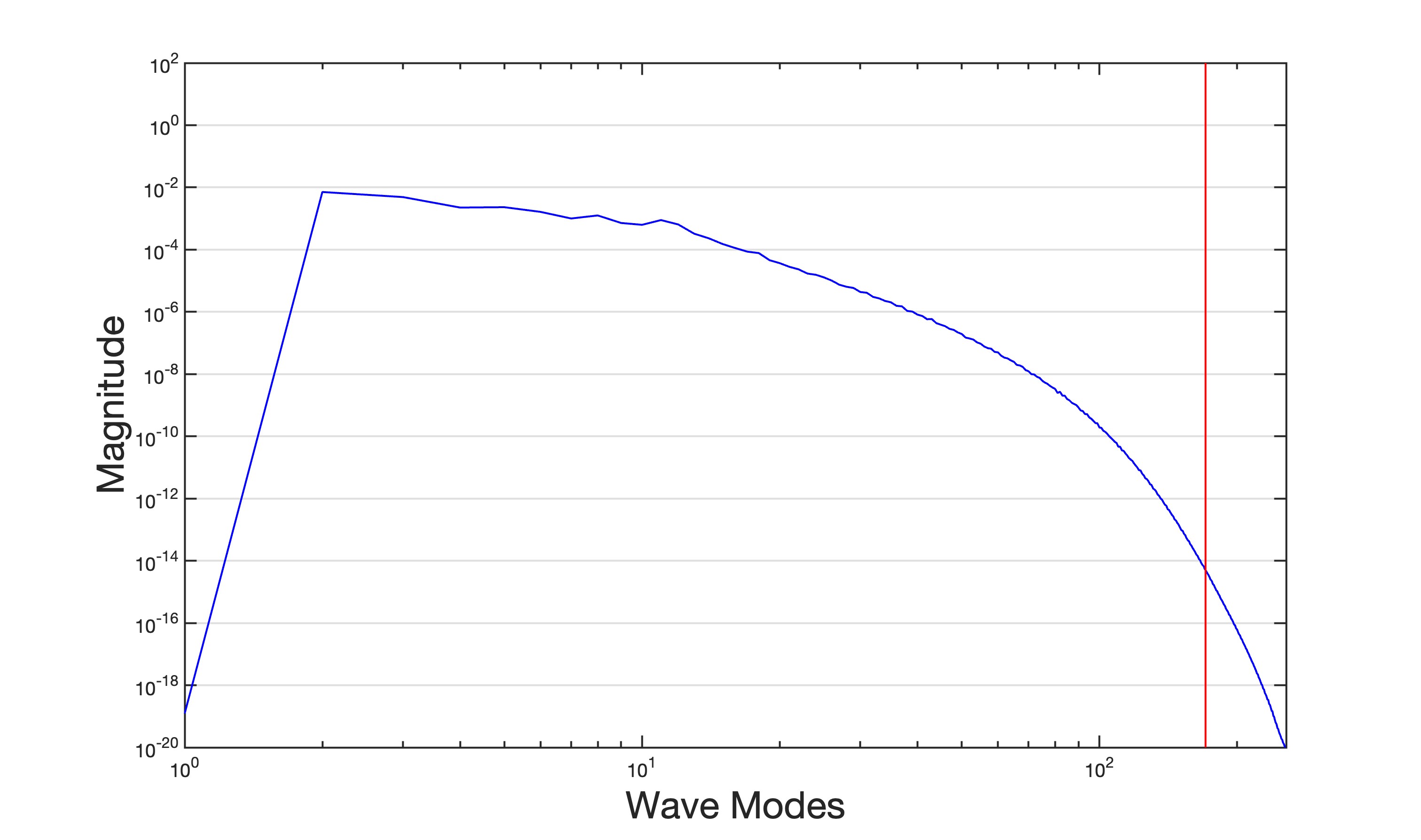
Figure 1. Energy spectrum of the initial data with $\nu=0.005$, $G=100,000$, and $\Delta t=0.001$. The vertical red line is the 2/3 dealiasing cutoff as $\frac{2}{3}\frac{N}{2}=170.\overline{6}.$

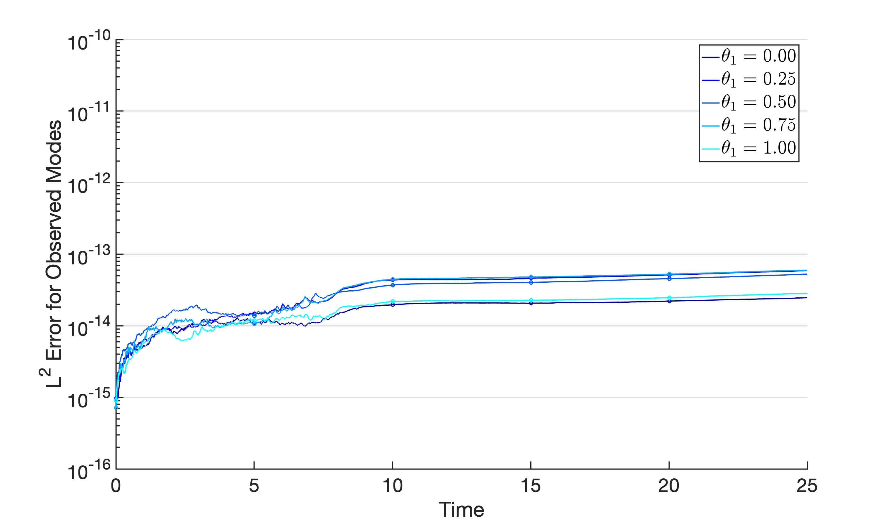
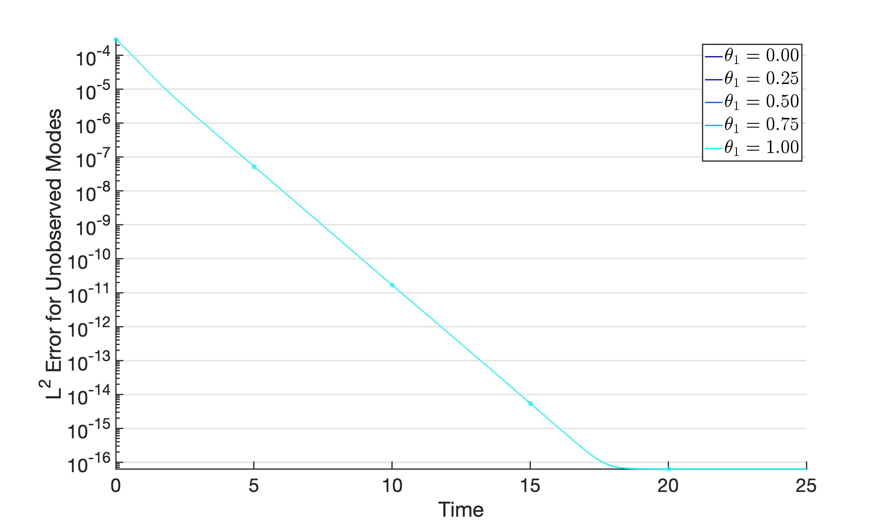
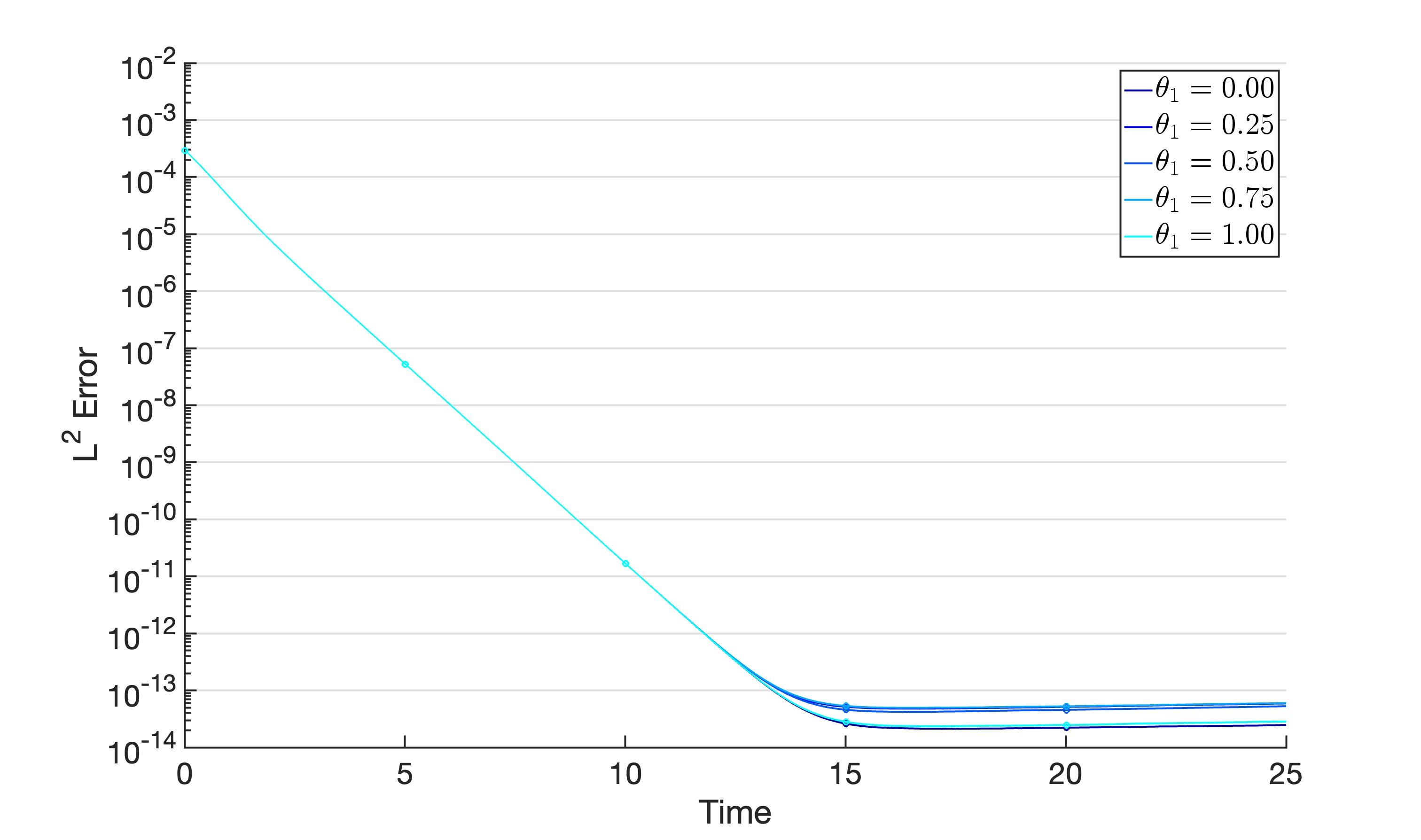
Figure 2. Error over time for different $\theta_{1}$ values for mutual synchronization. Here $v_{2}(t_{0})=P_{N}(v_{1}(t_{0}))$.

6.3. Nudging Intertwinement

In this section, we describe an implementation of the nudging intertwinement equations (3.13) and present the subsequent results. We focus only on the mutual nudging intertwinement (3.14) and symmetric nudging intertwinement (3.15). For these intertwinements, we again implement intertwined system according to (6.1), but with the additional terms coming from the intertwining functions computed explicitly. We simulated these equations for various instances of the intertwining matrix, $M$, using spatial resolution, $N=2^{9}$ and viscosity $\nu=0.0005$. We again consider $g_{1}=g_{2}=f$, with $f$ being the time-independent forcing described in Section 6.1.

To initialize our equations we used a solution to 2D NSE that had been spun up from initial data $0$ up to time $10,000$. To generate the second initial profile we evolved this solution out an additional $100$ units of time at which point we found that the solutions appeared to be sufficiently decorrelated. This decorrelation can be observed in the error at the initial times in Figure 3, Figure 4, and Figure 6.

6.3.1. Mutual Nudging Intertwinement

For all of our simulations we fixed $\mu_{1}=50$ and varied $0\leq\mu_{2}\leq\mu_{1}$. We found that when utilizing nonnegative $\mu_{2}$ that all of the simulations behaved approximately the same way. In each case, we obtained exponential convergence of $v_{1}$ to $v_{2}$ at approximately the same rate. We observe the exponential decay in the error, split into the observed and unobserved modes, in Figure 3, where the plots are nearly indistinguishable. Upon zooming in on the initial development of the error, we see in Figure 4 that the error converges exponentially in the initial period at rates which increase as $\mu_{2}$ increases in the initial period, before they transitions to a slower, but nevertheless exponential, decay rate.

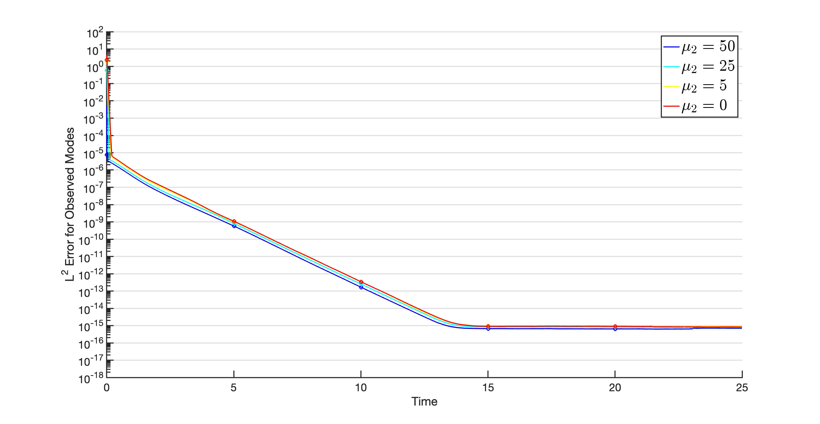
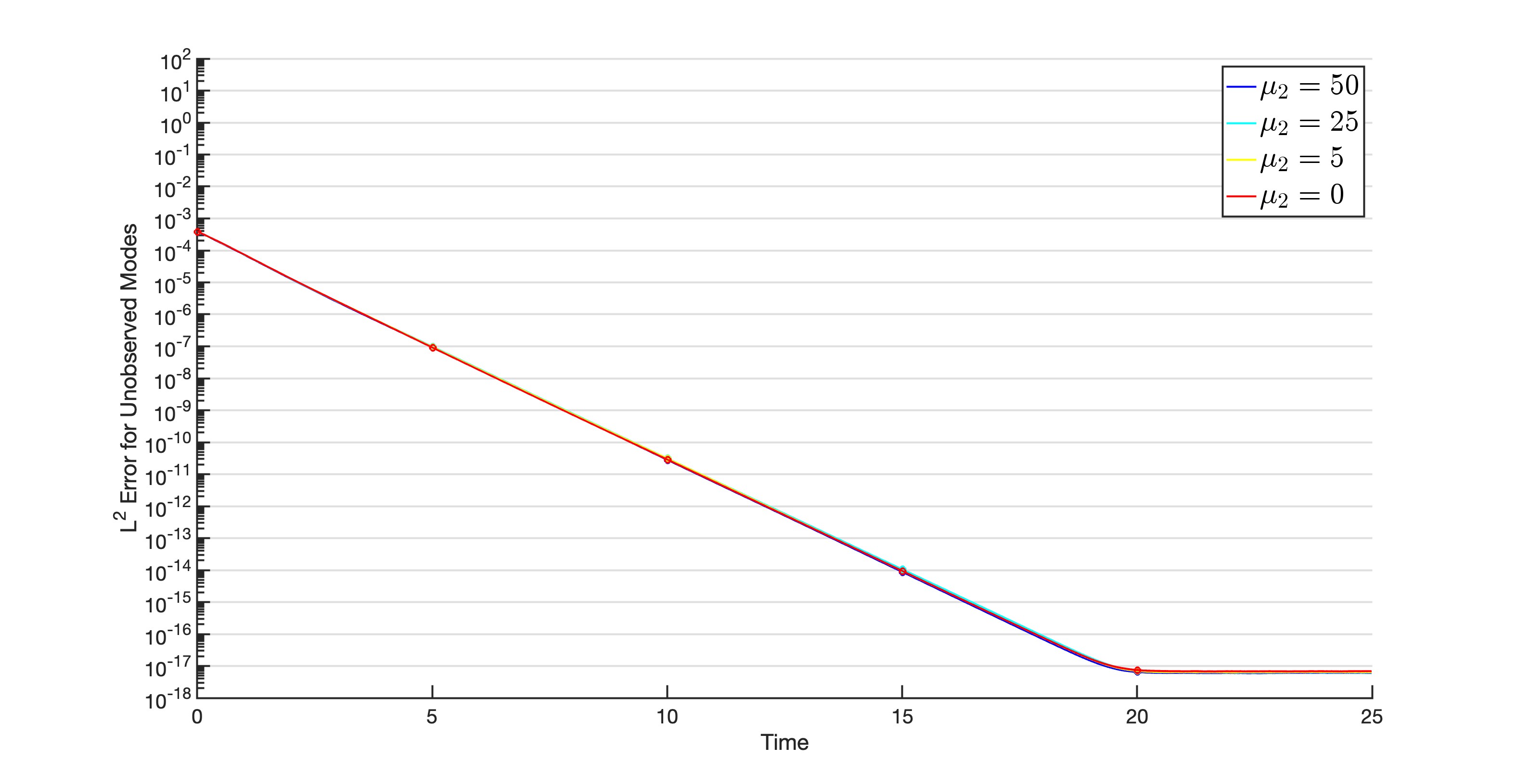
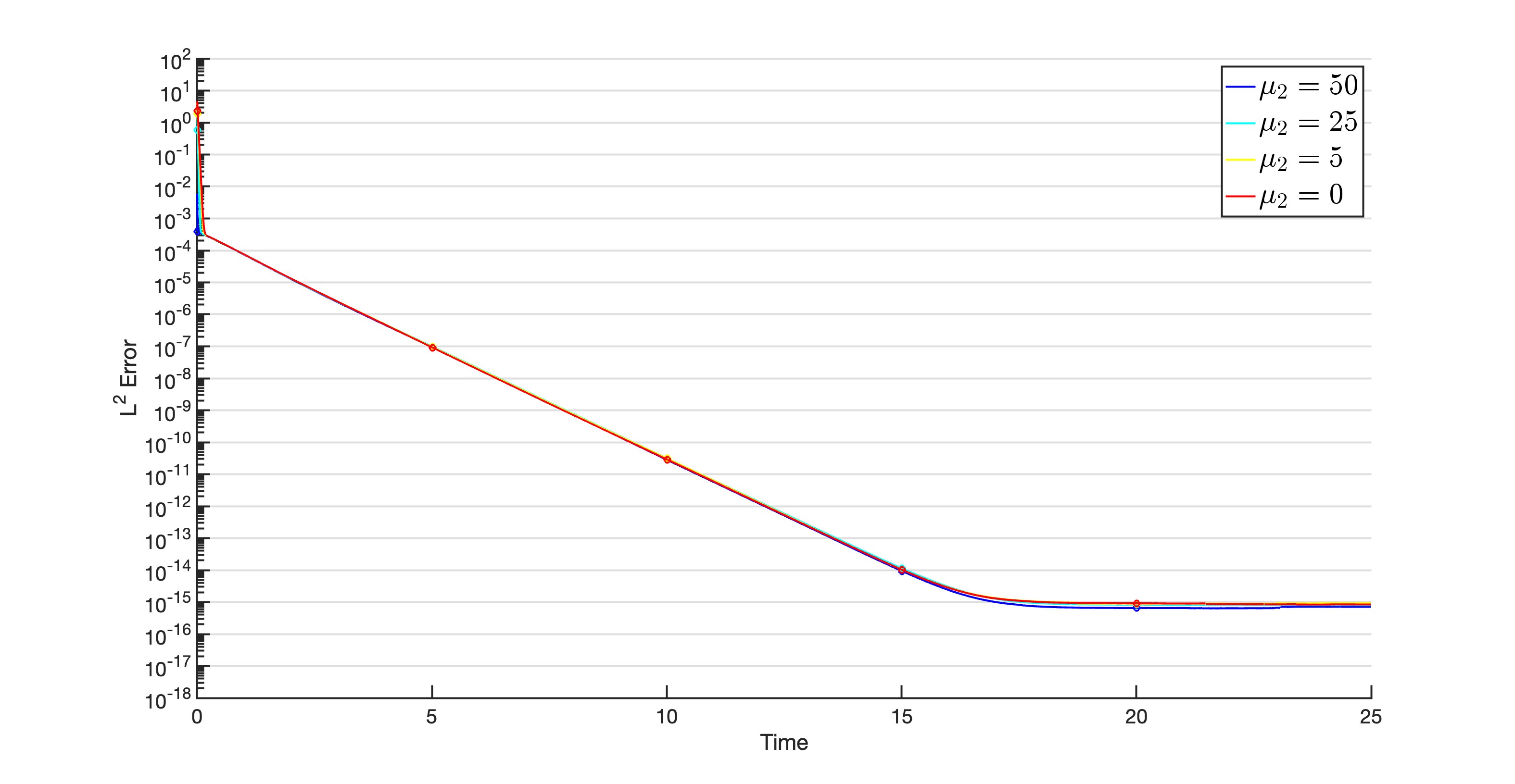
Figure 3. Error over time for mutual nudging intertwinements with $\mu_{1}=50$ and various non-negative values for $\mu_{2}$.

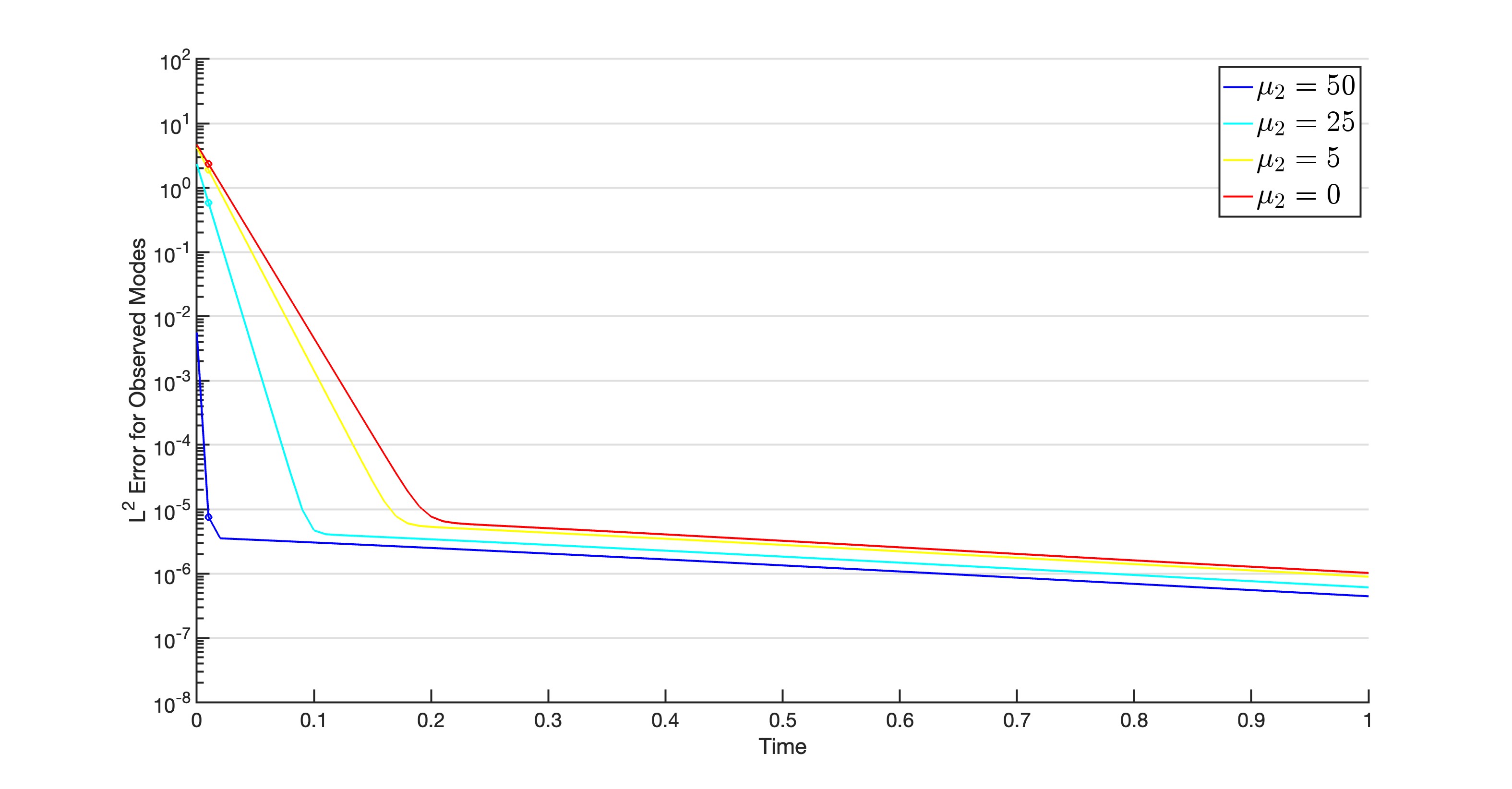
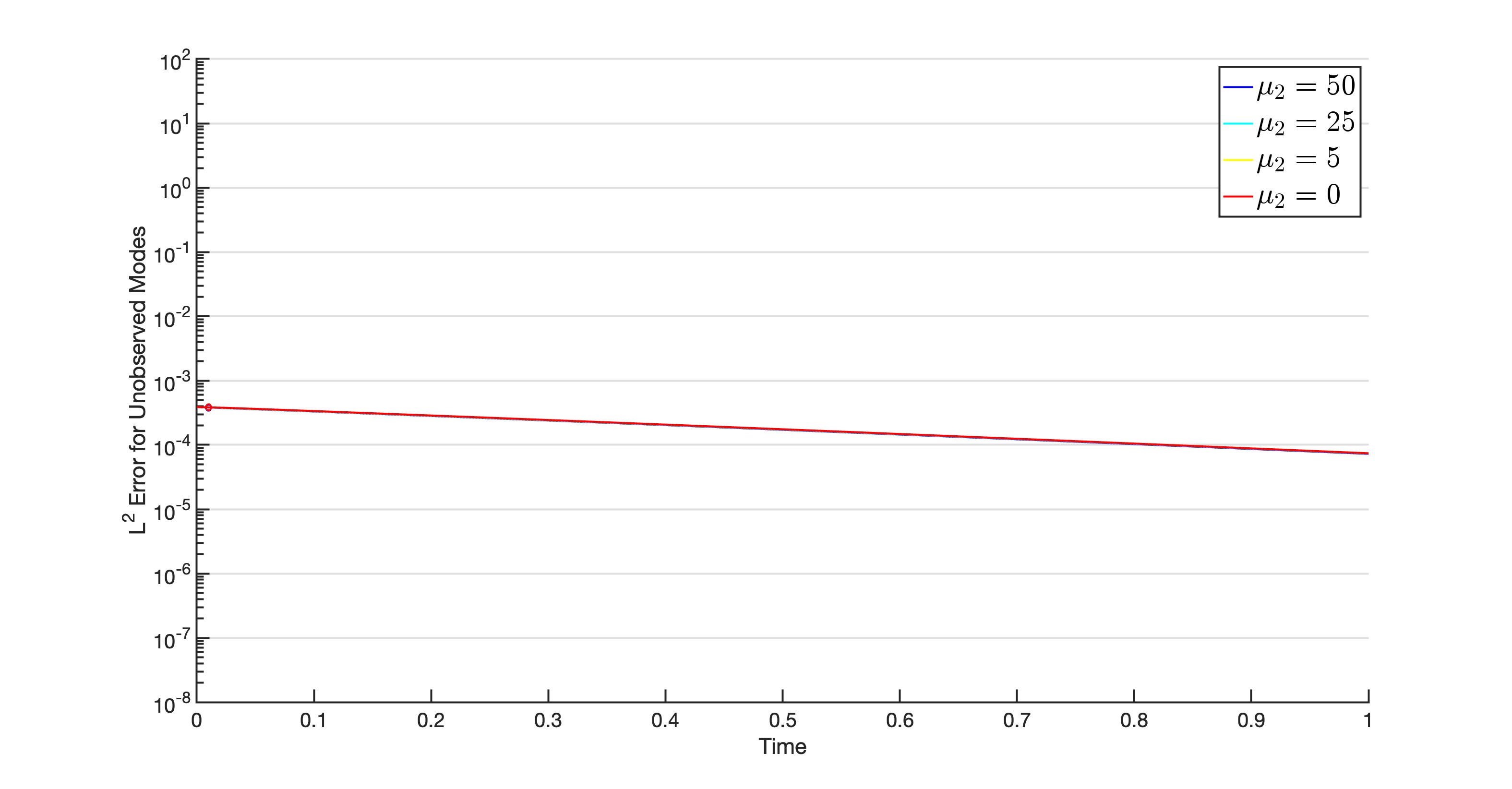
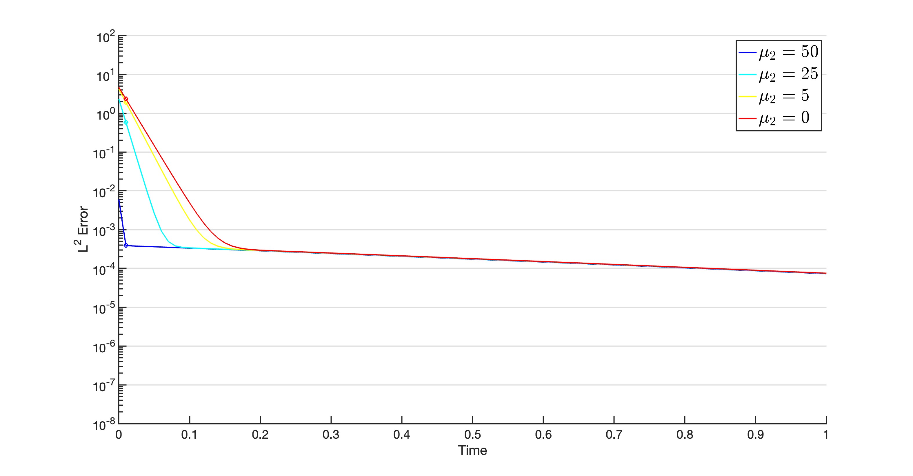
Figure 4. Error over time for mutual nudging intertwinements with $\mu_{1}=50$ and various non-negative values for $\mu_{2}$. Zoomed in plot showing initial error development for Figure 3

6.3.2. Symmetric Nudging Intetwinement

For all of our simulations, we once again fixed $\mu_{1}=50$ and varied $0\leq\mu_{2}\leq\mu_{1}$. We found that all of the simulations behaved approximately the same, except for when $\mu_{1}=\mu_{2}$, which is precisely when the smallest value of the eigenvalues of the intertwining matrix is zero (see (5.75), (5.82)). We see that in each case, except when $\mu_{1}=\mu_{2}$, we obtained exponential convergence of $v_{1}$ to $v_{2}$ at approximately the same rate. In the case when $\mu_{1}=\mu_{2}$ we nevertheless still obtained exponential synchronization between $v_{1}$ and $v_{2}$, but it occurred at a different rate than the other cases; this quality is found in both the “observed” and “unobserved” modes. The exponential decay in the error, split into the observed and unobserved modes, is presented in Figure 5, where the plots are once again nearly indistinguishable. Upon zooming in on the early development of the error (Figure 6), we see that in each method, the cases where $\mu_{2}\neq\mu_{1}$ initially exhibit a different rate of synchronization before quickly transitioning to a slower, but nevertheless exponential, decay rate.

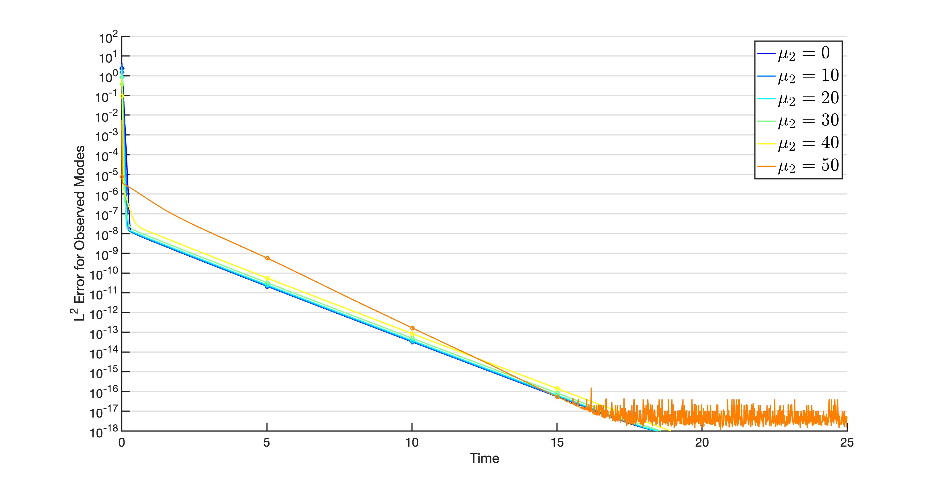
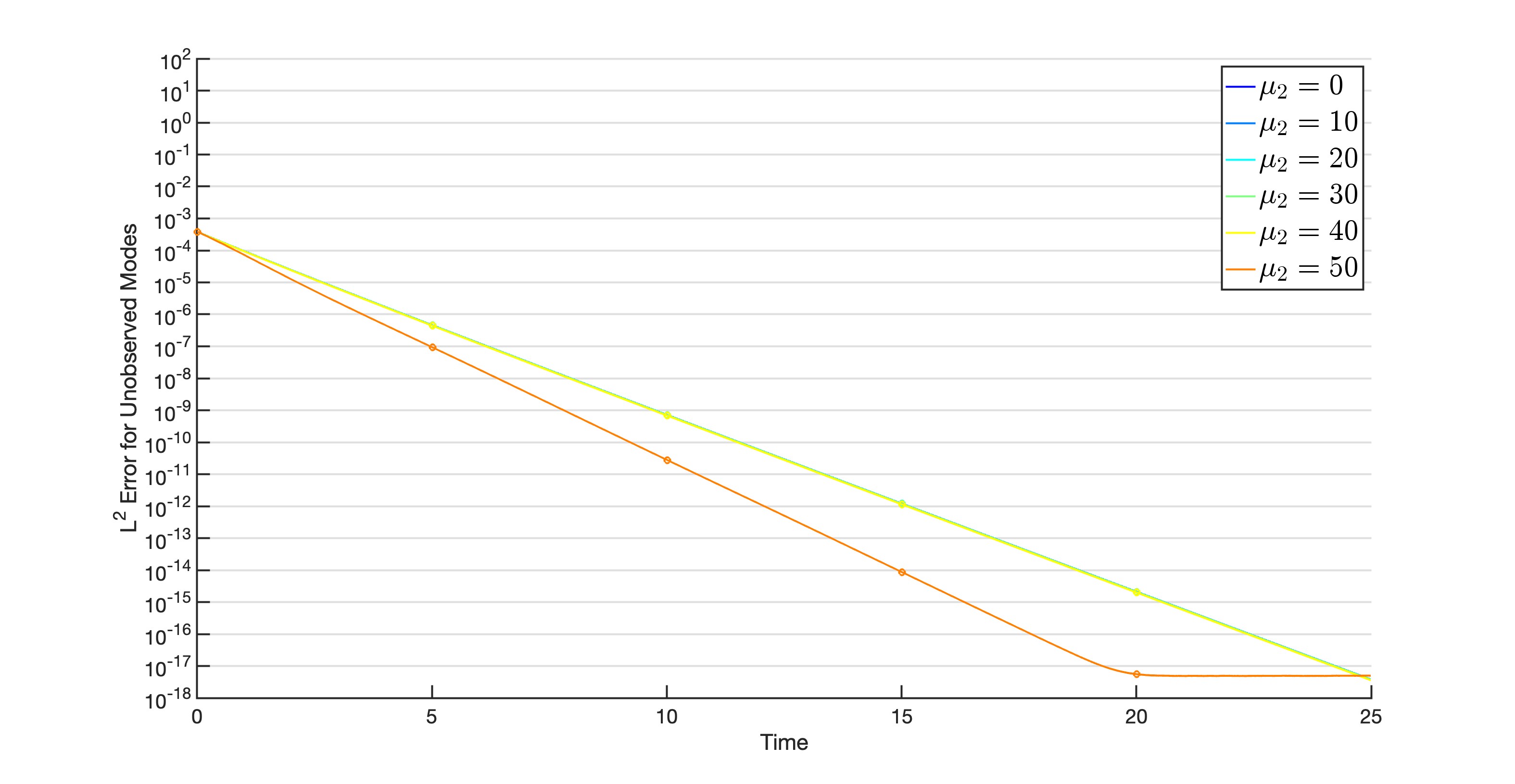
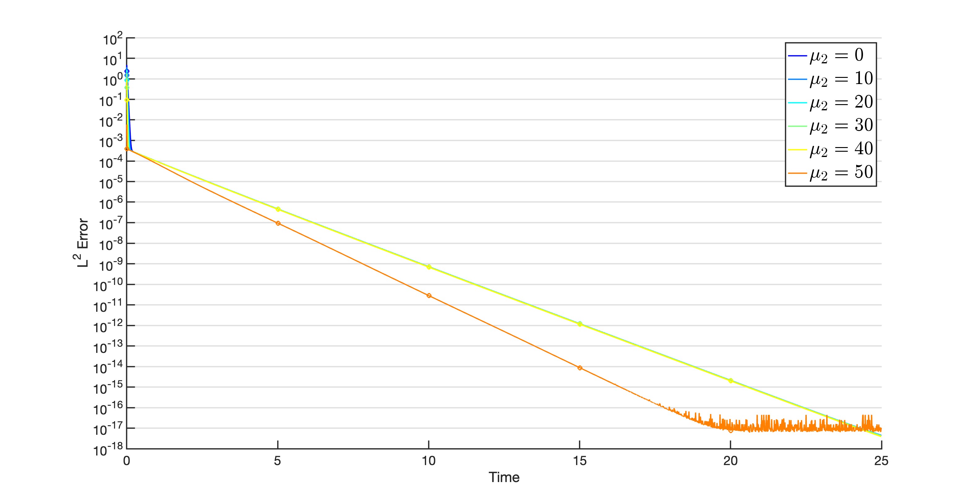
Figure 5. Error over time for symmetric nudging intertwinements with $\mu_{1}=50$ and various non-negative values for $\mu_{2}$.

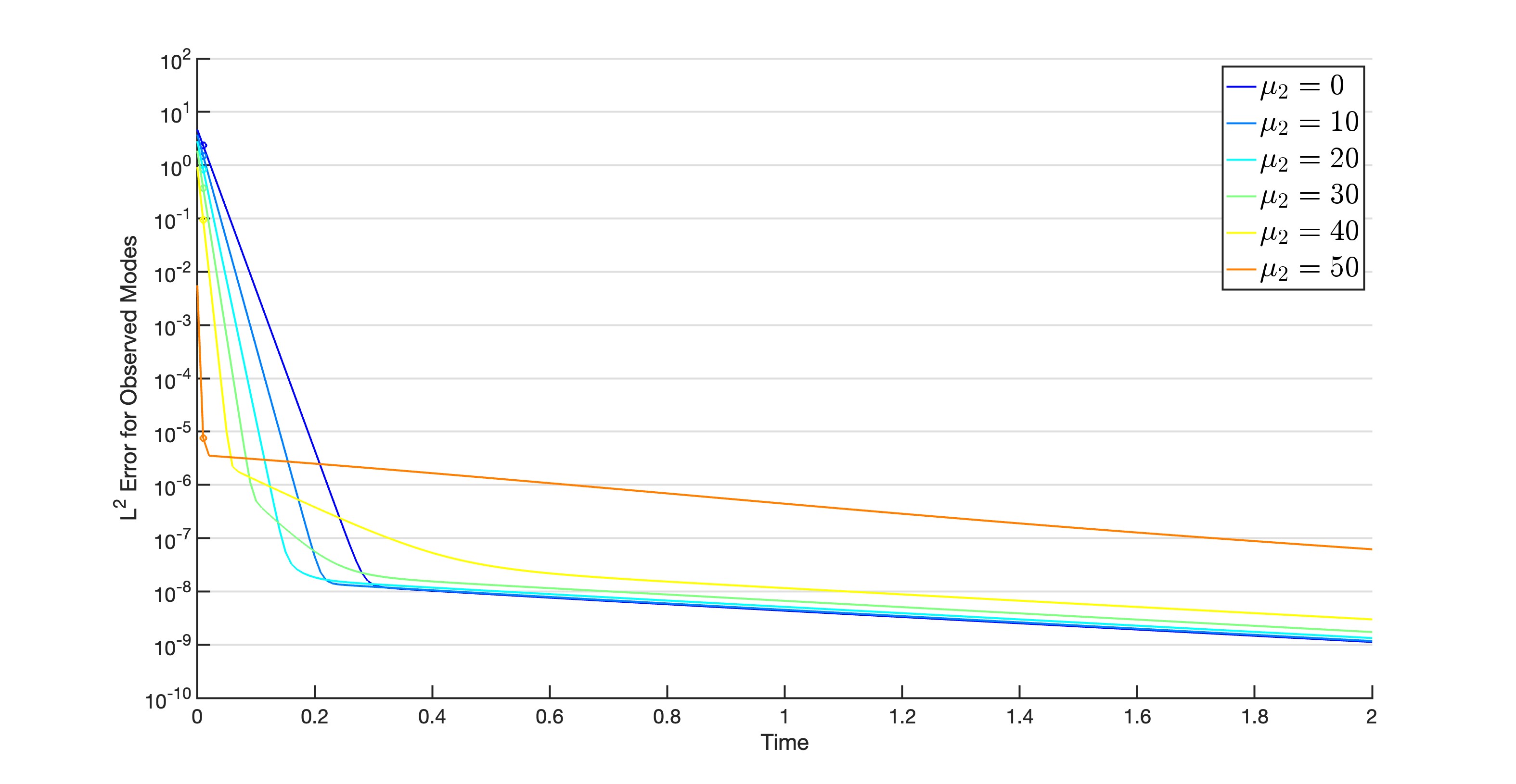
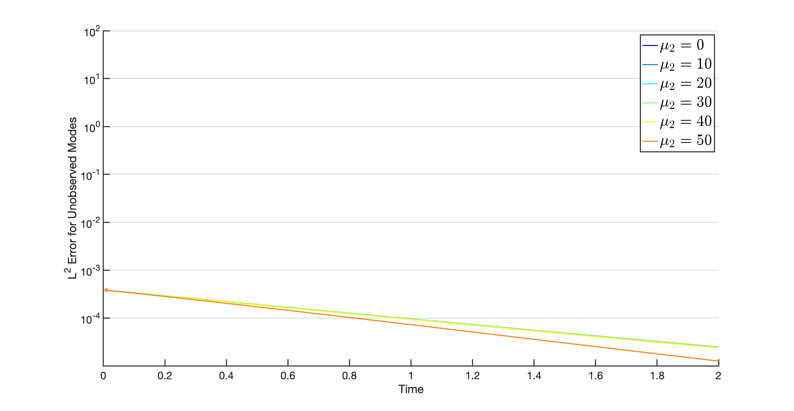
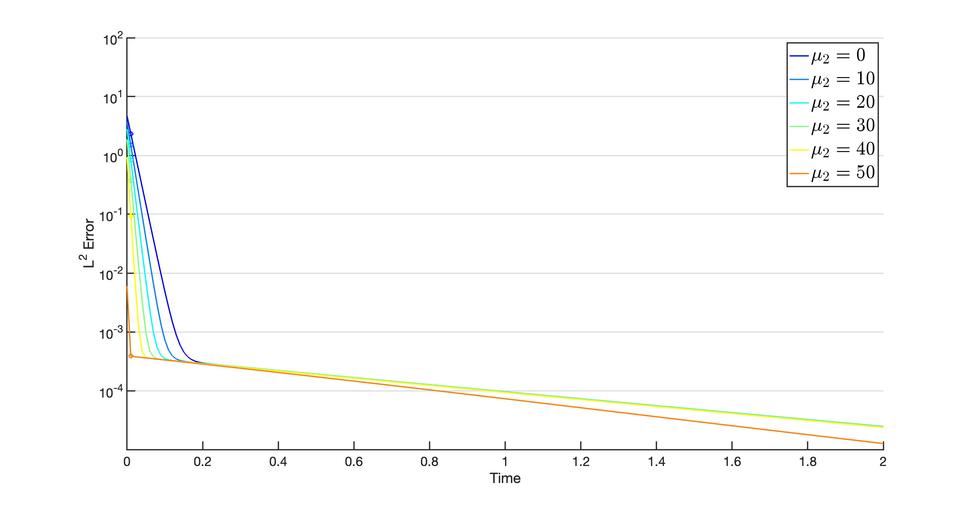
Figure 6. Error over time for symmetric nudging intertwinements with $\mu_{1}=50$ and various non-negative values for $\mu_{2}$. Zoomed in plot showing initial error development for Figure 5

Acknowledgments

The authors would like to thank Edriss Titi for stimulating discussions related to this work. A.F. was supported in part by the National Science Foundation through DMS 2206493. V.R.M. was in part supported by the National Science Foundation through DMS 2213363 and DMS 2206491, as well as the Dolciani Halloran Foundation.

Elizabeth Carlson
Department of Computing & Mathematical Sciences
California Institute of Technology
Web: https://sites.google.com/view/elizabethcarlsonmath
Email: elizcar@caltech.edu

Aseel Farhat
Department of Mathematics
Florida State University
Email: afarhat@fsu.edu
Department of Mathematics
University of Virginia
Email: af7py@virginia.edu

Vincent R. Martinez
Department of Mathematics & Statistics
CUNY Hunter College
Department of Mathematics
CUNY Graduate Center
Web: http://math.hunter.cuny.edu/vmartine/
Email: vrmartinez@hunter.cuny.edu

Collin Victor
Department of Mathematics
Texas A&M University
Web: https://www.math.tamu.edu/people/formalpg.php?user=collin.victor
Email: collin.victor@tamu.edu

References

- [AB24] D. A. F. Albanez and M.J. Benvenutti, Parameter analysis in continuous data assimilation for three-dimensional brinkman–forchheimer-extended darcy model, Partial Differential Equations and Applications 5 (2024), no. 4, 23.
- [ANLT16] D.A.F. Albanez, H.J. Nussenzveig Lopes, and E.S. Titi, Continuous data assimilation for the three-dimensional Navier-Stokes- model, Asymptotic Anal. 97 (2016), no. 1-2, 165–174.
- [AOT14] A Azouani, E.J. Olson, and E.S. Titi, Continuous data assimilation using general interpolant observables, J. Nonlinear Sci. 24 (2014), no. 2, 277–304.
- [ATG+17] M.U. Altaf, E.S. Titi, T. Gebrael, O.M. Knio, L. Zhao, and M.F. McCabe, Downscaling the 2d Bénard convection equations using continuous data assimilation, Comput. Geosci. 21 (2017), 393–410.
- [BBJ21] A. Biswas, Z. Bradshaw, and M.S. Jolly, Data assimilation for the navier–stokes equations using local observables, SIAM Journal on Applied Dynamical Systems 20 (2021), no. 4, 2174–2203.
- [BCT+22] H. Bercovici, P. Constantin, A. Tannenbaum, R. Temam, and E.S. Titi, Remembrances of ciprian ilie foias, AMS Notices 69 (2022), no. 9, 1529–1545.
- [BFMT19] A. Biswas, C. Foias, C.F. Mondaini, and E.S. Titi, Downscaling data assimilation algorithm with applications to statistical solutions of the navier–stokes equations, Annales de l’Institut Henri Poincaré C, Analyse non linéaire 36 (2019), no. 2, 295–326.
- [BFZ23] Z. Brzeźniak, B. Ferrario, and M. Zanella, Ergodic results for the stochastic nonlinear schrödinger equation with large damping, Journal of Evolution Equations 23 (2023), no. 1, 19.
- [BH23] A. Biswas and J. Hudson, Determining the viscosity of the navier–stokes equations from observations of finitely many modes, Inverse Problems 39 (2023), no. 12, 125012.
- [BKS20] O. Butkovsky, A. Kulik, and M. Scheutzow, Generalized couplings and ergodic rates for spdes and other markov models, The Annals of Applied Probability 30 (2020), no. 1, pp. 1–39.
- [BLSZ13] D. Blömker, K. Law, A. M. Stuart, and K. C. Zygalakis, Accuracy and stability of the continuous-time 3DVAR filter for the Navier-Stokes equation, Nonlinearity 26 (2013), no. 8, 2193–2219.
- [CBK23] G. Carigi, J. Bröcker, and T. Kuna, Exponential ergodicity for a stochastic two-layer quasi-geostrophic model, Stochastics and Dynamics 23 (2023), no. 02, 2350011.
- [CDLMB18] P. Clark Di Leoni, A. Mazzino, and L. Biferale, Inferring flow parameters and turbulent configuration with physics-informed data assimilation and spectral nudging, Phys. Rev. Fluids 3 (2018), no. 10, 104604.
- [CDS03] I. Chueshov, J. Duan, and B. Schmalfuss, Determining functionals for random partial differential equations, Nonlinear Differential Equations and Applications NoDEA 10 (2003), no. 4, 431–454.
- [CFMT85] P. Constantin, C. Foias, O. P. Manley, and R. Temam, Determining modes and fractal dimension of turbulent flows, Journal of Fluid Mechanics 150 (1985), 427–440.
- [CFT88] P. Constantin, C. Foias, and R. Temam, On the dimension of the attractors in two-dimensional turbulence, Phys. D 30 (1988), 284–296.
- [CHL20] E. Carlson, J. Hudson, and A. Larios, Parameter recovery for the 2 dimensional Navier-Stokes equations via continuous data assimilation, SIAM J. Sci. Comput. 42 (2020), no. 1, A250–A270.
- [CHL+22] E. Carlson, J. Hudson, A. Larios, V.R. Martinez, E. Ng, and J.P. Whitehead, Dynamically learning the parameters of a chaotic system using partial observations, Discrete and Continuous Dynamical Systems 42 (2022), no. 8, 3809–3839.
- [CJT97] B. Cockburn, D.A. Jones, and E.S. Titi, Estimating the number of asymptotic degrees of freedom for nonlinear dissipative systems, Math. Comput. 66 (1997), 1073–1087.
- [CO23] E. Celik and E. Olson, Data assimilation using time-delay nudging in the presence of gaussian noise, Journal of Nonlinear Science 33 (2023), no. 6, 110.
- [COT19] E. Celik, E. Olson, and E.S. Titi, Spectral filtering of interpolant observables for a discrete-in-time downscaling data assimilation algorithm, SIAM J. Appl. Dyn. Syst. 18 (2019), no. 2, 1118–1142. MR 3959540
- [Deb13] A. Debussche, Ergodicity results for the stochastic navier–stokes equations: An introduction, pp. 23–108, Springer Berlin Heidelberg, Berlin, Heidelberg, 2013.
- [DLMB18] P. Di Leoni, A. Mazzino, and L. Biferale, Inferring flow parameters and turbulent configuration with physics-informed data assimilation and spectral nudging, Phys. Rev. Fluids 3 (2018), 104604.
- [DO05] A. Debussche and C. Odasso, Ergodicity for a weakly damped stochastic non-linear Schrödinger equation, J. Evol. Equ. 5 (2005), no. 3, 317–356. MR 2174876
- [EMS01] W. E, J. C. Mattingly, and Y. G.. Sinai, Gibbsian dynamics and ergodicity for the stochastically forced Navier-Stokes equation, Comm. Math. Phys. 224 (2001), no. 1, 83–106, Dedicated to Joel L. Lebowitz. MR 1868992 (2002m:76024)
- [FDKT14] K. Foyash, M. S. Dzholli, R. Kravchenko, and È. S. Titi, A unified approach to the construction of defining forms for a two-dimensional system of Navier–Stokes equations: the case of general interpolating operators, Uspekhi Mat. Nauk 69 (2014), no. 2(416), 177–200.
- [FJJT18] A. Farhat, H. Johnston, M.S. Jolly, and E.S. Titi, Assimilation of nearly turbulent Rayleigh-Bénard flow through vorticity or local circulation measurements: A computational study, J. Sci. Comput. (2018), 1–15.
- [FJKT12] C. Foias, M.S. Jolly, R. Kravchenko, and E.S. Titi, A determining form for the two-dimensional Navier-Stokes equations: the Fourier modes case, J. Math. Phys. 53 (2012), no. 11, 115623, 30.
- [FJLT17] C. Foias, M.S. Jolly, D. Lithio, and E.S. Titi, One-dimensional parametric determining form for the two-dimensional Navier-Stokes equations, J. Nonlinear Sci. 27 (2017), no. 5, 1513–1529.
- [FJT15] A. Farhat, M.S. Jolly, and E.S. Titi, Continuous data assimilation for the 2d Bénard convection through velocity measurements alone, Phys. D 303 (2015), 59–66.
- [FL99] F. Flandoli and J.A. Langa, Determining modes for dissipative random dynamical systems, Stochastics and Stochastic Reports 66 (1999), no. 1-2, 1–25.
- [FLMW24] Aseel Farhat, Adam Larios, Vincent R. Martinez, and Jared P. Whitehead, Identifying the body force from partial observations of a two-dimensional incompressible velocity field, Phys. Rev. Fluids 9 (2024), 054602.
- [FMT16] C. Foias, C. Mondaini, and E.S. Titi, A discrete data assimilation scheme for the solutions of the 2d Navier-Stokes equations and their statistics, SIAM J. Appl. Dyn. Syst. 15 (2016), no. 4, 2019–2142.
- [FMTT83] C. Foias, O. P. Manley, R. Temam, and Y. M. Treve, Number of modes governing two-dimensional viscous, incompressible flows, Phys. Rev. Lett. 50 (1983), 1031–1034.
- [FP67] C. Foiaş and G. Prodi, Sur le comportement global des solutions non-stationnaires des équations de Navier-Stokes en dimension , Rend. Sem. Mat. Univ. Padova 39 (1967), 1–34.
- [FT79] C. Foias and T. Temam, Some analytic and geometric properties of the solutions of the evolution of the Navier-Stokes equations, J. Math. Pures Appl. 9 (1979), no. 58, 339–368.
- [FT84] C. Foias and R. Temam, Determination of the solutions of the Navier-Stokes equations by a set of nodal values, Math. Comput. 43 (1984), no. 167, 117–133.
- [FT87] by same author, The connection between the Navier-Stokes equations, dynamical systems, and turbulence theory, Directions in partial differential equations (Madison, WI, 1985), Publ. Math. Res. Center Univ. Wisconsin, vol. 54, Academic Press, Boston, MA, 1987, pp. 55–73. MR 1013833
- [FT91] C Foias and E S Titi, Determining nodes, finite difference schemes and inertial manifolds, Nonlinearity 4 (1991), no. 1, 135.
- [FZ23] B. Ferrario and M. Zanella, Uniqueness of the invariant measure and asymptotic stability for the 2d navier stokes equations with multiplicative noise, 2023, pp. 1–32.
- [GALNR24] B. García-Archilla, X. Li, J. Novo, and L.G. Rebholz, Enhancing nonlinear solvers for the navier–stokes equations with continuous (noisy) data assimilation, Computer Methods in Applied Mechanics and Engineering 424 (2024), 116903.
- [GAN20] B. García-Archilla and J. Novo, Error analysis of fully discrete mixed finite element data assimilation schemes for the navier-stokes equations, Advances in Computational Mathematics 46 (2020), no. 4, 61.
- [GHMN22] N.E. Glatt-Holtz, V.R. Martinez, and H.D. Nguyen, The short memory limit for long time statistics in a stochastic coleman-gurtin model of heat conduction, 2022, pp. 1–71.
- [GHMR17] N. Glatt-Holtz, J.C. Mattingly, and G. Richards, On unique ergodicity in nonlinear stochastic partial differential equations, J. Stat. Phys. 166 (2017), no. 3-4, 618–649.
- [GHMR21] Nathan Glatt-Holtz, Vincent R Martinez, and Geordie H Richards, On the long-time statistical behavior of smooth solutions of the weakly damped, stochastically-driven KdV equation, arXiv preprint arXiv:2103.12942 (2021), 1–74.
- [HM06] M. Hairer and J. C. Mattingly, Ergodicity of the 2D Navier-Stokes equations with degenerate stochastic forcing, Ann. of Math. (2) 164 (2006), no. 3, 993–1032. MR 2259251 (2008a:37095)
- [HMS11] M. Hairer, J. C. Mattingly, and M. Scheutzow, Asymptotic coupling and a general form of Harris’ theorem with applications to stochastic delay equations, Probab. Theory Related Fields 149 (2011), no. 1-2, 223–259. MR 2773030
- [HOT11] K. Hayden, E. Olson, and E.S. Titi, Discrete data assimilation in the Lorenz and 2D Navier-Stokes equations, Phys. D 240 (2011), no. 18, 1416–1425. MR 2831793
- [HTHK22] M.A.E.R. Hammoud, E.S. Titi, I. Hoteit, and O. Knio, Cdanet: A physics-informed deep neural network for downscaling fluid flows, Journal of Advances in Modeling Earth Systems 14 (2022), no. 12, e2022MS003051, e2022MS003051 2022MS003051.
- [IMT19] H.A. Ibdah, C.F. Mondaini, and E.S. Titi, Fully discrete numerical schemes of a data assimilation algorithm: uniform-in-time error estimates, IMA Journal of Numerical Analysis 40 (2019), no. 4, 2584–2625.
- [JMST18] M.S. Jolly, V.R. Martinez, S. Sadigov, and E.S. Titi, A Determining Form for the Subcritical Surface Quasi-Geostrophic Equation, J. Dyn. Differ. Equations (2018), 1–38.
- [JMT17] M.S. Jolly, V.R. Martinez, and E.S. Titi, A data assimilation algorithm for the 2d subcritical surface quasi-geostrophic equation, Adv. Nonlinear Stud. 35 (2017), 167–192.
- [JP23] M.S. Jolly and A. Pakzad, Data assimilation with higher order finite element interpolants, International Journal for Numerical Methods in Fluids 95 (2023), no. 3, 472–490.
- [JST15] M.S. Jolly, T. Sadigov, and E.S. Titi, A determining form for the damped driven nonlinear schrödinger equation–fourier modes case, J. Differential Equations 258 (2015), 2711–2744.
- [JST17] by same author, Determining form and data assimilation algorithm for weakly damped and driven korteweg-de vries equation- fourier modes case, Nonlinear Anal. Real World Appl. 36 (2017), 287–317.
- [JT92a] D.A. Jones and E.S. Titi, Determining finite volume elements for the 2d navier-stokes equations, Phys. D 60 (1992), 165–174.
- [JT92b] by same author, On the number of determining nodes for the 2d Navier-Stokes equations, J. Math. Anal. 168 (1992), 72–88.
- [KEML+24] E.D. Koronaki, N. Evangelou, C.P. Martin-Linares, E.S. Titi, and I.G. Kevrekidis, Nonlinear dimensionality reduction then and now: Aims for dissipative pdes in the ml era, Journal of Computational Physics 506 (2024), 112910.
- [KKZ23] V. Kalantarov, A. Kostianko, and S. Zelik, Determining functionals and finite-dimensional reduction for dissipative PDEs revisited, J. Differential Equations 345 (2023), 78–103. MR 4513832
- [KS00] S. Kuksin and A. Shirikyan, Stochastic dissipative PDEs and Gibbs measures, Comm. Math. Phys. 213 (2000), no. 2, 291–330. MR 1785459
- [KS12] by same author, Mathematics of two-dimensional turbulence, Cambridge Tracts in Mathematics, no. 194, Cambridge University Press, 2012.
- [KT05] Aly-Khan Kassam and Lloyd N. Trefethen, Fourth-order time-stepping for stiff PDEs, SIAM J. Sci. Comput. 26 (2005), no. 4, 1214–1233. MR 2143482
- [Lad85] O. A. Ladyzhenskaya, Finite-dimensionality of bounded invariant sets for navier-stokes systems and other dissipative systems, Journal of Soviet Mathematics 28 (1985), no. 5, 714–726.
- [Lan03] J.A. Langa, Finite-dimensional limiting dynamics of random dynamical systems, Dynamical Systems 18 (2003), no. 1, 57–68.
- [Lor63] E. N. Lorenz, Deterministic nonperiodic flow, Journal of the Atmospheric Sciences 20 (1963), 130–141.
- [LRZ19] A. Larios, L.G. Rebholz, and C. Zerfas, Global in time stability and accuracy of IMEX-FEM data assimilation schemes for Navier-Stokes equations, Comput. Methods Appl. Mech. Engrg. 345 (2019), 1077–1093. MR 3912985
- [Mar22] V.R. Martinez, Convergence analysis of a viscosity parameter recovery algorithm for the 2D Navier-Stokes equations, Nonlinearity 35 (2022), no. 5, 2241–2287. MR 4420613
- [Mar24] by same author, On the reconstruction of unknown driving forces from low-mode observations in the 2d navier–stokes equations, Proc. R. Soc. Edinb. A: Math (2024), 1–24.
- [MT18] C.F. Mondaini and E.S. Titi, Uniform-in-time error estimates for the postprocessing galerkin method applied to a data assimilation algorithm, SIAM J. Numer. Anal. 56 (2018), no. 1, 78–110.
- [Ngu23] H.D. Nguyen, Ergodicity of a nonlinear stochastic reaction–diffusion equation with memory, Stochastic Processes and their Applications 155 (2023), 147–179.
- [OBK18] L. Oljača, J. Bröcker, and T. Kuna, Almost sure error bounds for data assimilation in dissipative systems with unbounded observation noise, SIAM Journal on Applied Dynamical Systems 17 (2018), no. 4, 2882–2914.
- [Oda06] C. Odasso, Ergodicity for the stochastic complex Ginzburg-Landau equations, Ann. Inst. H. Poincaré Probab. Statist. 42 (2006), no. 4, 417–454. MR 2242955
- [OT03] E. Olson and E.S. Titi, Determining modes for continuous data assimilation in 2D turbulence, J. Statist. Phys. 113 (2003), no. 5-6, 799–840, Progress in statistical hydrodynamics (Santa Fe, NM, 2002). MR 2036872
- [OT08a] Eric Olson and Edriss Titi, Determining modes and Grashof number in 2D turbulence: A numerical case study, Theor. Comput. Fluid Dyn. 22 (2008), 327–339.
- [OT08b] Eric Olson and Edriss S. Titi, Determining modes and grashof number in 2D turbulence: a numerical case study, Theor. Comp. Fluid Dyn. 22 (2008), no. 5, 327–339.
- [PWM22] B. Pachev, J.P. Whitehead, and S.A. McQuarrie, Concurrent multiparameter learning demonstrated on the kuramoto–sivashinsky equation, SIAM Journal on Scientific Computing 44 (2022), no. 5, A2974–A2990.
- [Rob01] James C. Robinson, Infinite-Dimensional Dynamical Systems, Cambridge Texts in Applied Mathematics, Cambridge University Press, Cambridge, 2001, An introduction to dissipative parabolic PDEs and the theory of global attractors. MR 1881888
- [Shi08] A. Shirikyan, Exponential mixing for randomly forced partial differential equations: Method of coupling, pp. 155–188, Springer New York, New York, NY, 2008.
- [Tre00] L.N. Trefethen, Spectral Methods in MATLAB, Software, Environments, and Tools, vol. 10, Society for Industrial and Applied Mathematics (SIAM), Philadelphia, PA, 2000. MR 1776072
- [YGJP22] C. Yu, A. Giorgini, M.S. Jolly, and A. Pakzad, Continuous data assimilation for the 3d ladyzhenskaya model: analysis and computations, Nonlinear Analysis: Real World Applications 68 (2022), 103659.
- [ZRSI19] C. Zerfas, L.G. Rebholz, M. Schneier, and T. Iliescu, Continuous data assimilation reduced order models of fluid flow, Computer Methods in Applied Mechanics and Engineering 357 (2019), 112596.