Analysis of Microhubs for Three-Sided Meal Delivery Services

Abstract

The rise of online meal delivery has led to a surge in delivery traffic to urban neighborhoods, resulting in issues such as increased traffic congestion, illegal parking, noise, and air pollution. This paper introduces and analyzes a novel meal delivery strategy that incorporates a microhub. In this approach, the service area is segmented into smaller sub-areas, with deliverers assigned to operate exclusively within these sub-areas. The microhub functions as a transfer depot, enabling the batching and transfer of orders toward different sub-areas. To evaluate this system’s performance, two critical metrics—customer waiting time and vehicle miles traveled—are estimated through the continuous approximation approach. Comprehensive numerical experiments are conducted to validate the accuracy of our approximations. The derived analytical approximation is then integrated into an optimal design problem to determine the optimal number of sub-areas and the optimal batch size of packages within each sub-area. The numerical results suggest that the meal delivery system with a microhub outperforms the traditional pickup and delivery mode in both metrics, under either high demand or low supply conditions. The higher efficiency of the microhub design is attributed to the strategy of sub-regional batching, facilitated by the use of the microhub.

Keywords - meal delivery; microhub; pickup-and-delivery problems; continuous approximation; discrete-event simulation

1 Introduction

Meal delivery services connect customers and restaurants through mobile applications, allowing users to order meals online with just a few taps on their smartphones. The platform assigns meal orders to a team of affiliated deliverers, who complete the fulfillment process by picking up the meal package from the restaurant and delivering it to the customers. The lasting COVID-19 pandemic prompted an irreversible shift among consumers from indoor dining to online meal delivery Kaczmarski, (2024), under which takeout channels have become increasingly vital to restaurant operations in the post-pandemic era Shi and Xu, (2024). The significant surge in customer demand has heightened the need for meal delivery platforms to innovate supply management to ensure timely delivery. To prioritize customer satisfaction, platforms have been continuously seeking faster last-mile delivery methods, such as efficient batching and assignment strategies Liu et al., (2021); Simoni and Winkenbach, (2023), advanced vehicle routing strategies Steever et al., (2019); Kohar and Jakhar, (2021), and new delivery modes utilizing autonomous vehicles and drones Liu, (2019); Shi et al., (2022). As intermediaries in a three-sided service market involving customers, deliverers, and restaurants, meal delivery platforms must carefully consider and manage the differing interests of these stakeholders when introducing new delivery mechanisms Agatz et al., (2024).

This study conceptualizes a new design for meal delivery, utilizing microhubs as transshipment points, which demonstrates great potential for efficiency gains that potentially benefit all stakeholders in the long run. The concept of microhubs has been widely adopted in the context of e-commerce and last-mile delivery. A microhub functions as a logistical depot in urban neighborhoods for the collection, storage, and distribution of packages. It brings services closer to end customers and enables more flexible operations within targeted service areas. These microhubs help alleviate congestion, reduce emissions, consolidate freight vehicle trips, minimize vehicle miles traveled, and facilitate transfers to low- or zero-emission fleets for last-mile deliveries Gunes et al., (2024). In our proposed design for meal delivery, a service region can be divided into several small sub-areas, with the microhub acting as a temporary intermediate node facilitating the storage and transfer of meals between pickup and drop-off points and between different sub-areas. Individual meal packages are picked up from the restaurants where they originated and transported to the microhub. Subsequently, a different deliverer collects the package from the microhub and delivers it to the customer. Delivery vehicles are dispatched within each area to perform pickup, drop-off, and transfer tasks, with each vehicle dedicated to serving a specific sub-area. In practical implementation, deliverers possess better knowledge in routing for regions they are familiar with and prefer to operate exclusively within these areas for greater efficiency. However, in the context of more speed-sensitive meal delivery, an additional transshipment might delay order deliveries, resulting in customer dissatisfaction. In this study, we adopt continuous approximations (CA) to model meal delivery operations and estimate the average vehicle miles traveled and the average customer waiting time, both with and without transshipment at microhubs, to evaluate the comparative efficiency gains provided by setting up microhubs.

Compared to traditional optimization-based models used to address the vehicle routing problem with pickup and delivery (VRPPD) at the operational level Toth and Vigo, (2002), CA models are extensively applied to tackle big-picture questions about logistics and transportation systems Ansari et al., (2018). These applications include evaluating new designs in public transit Chen and Nie, 2017a ; Chen and Nie, 2017b and comparing new strategies with existing ones for dial-a-ride services Xu et al., (2020); Ouyang and Yang, (2023). While optimization-based approaches have significantly improved in solution quality over the past decade, their heavy formulations may fall short in providing a comprehensive understanding of the problem’s inherent characteristics, which could be critical for managerial insights. Additionally, concerns about data quality, particularly regarding precision and uncertainty, cast doubt on the reliability of optimal solutions in practical applications Daganzo, 1987b . CA models, serving as a complement to optimization models, have proven effective in addressing these challenges. According to (Daganzo et al.,, 2012), effective CA models can yield five major benefits: they require fewer data inputs, exhibit reduced computational complexity, provide enhanced system representation, improve transparency, and facilitate deeper insights.

For adopting the CA approach, the challenge lies in describing the system of interest as simply as possible while maintaining accurate estimations, a principle known as creating a parsimonious model. For a meal delivery system, its market conditions can be characterized primarily by three exogenous components: the coverage of service areas, the level of customer demand, and the service capacity provided by deliverers. Given specific market conditions, the platform will make strategic decisions on how to divide the area into smaller sub-areas as well as the strategy for batching and fulfilling pickup and drop-off requests within each sub-area. The system performances are influenced by both the exogenous market conditions and the operating strategy taken by the platform in fulfilling meal deliveries. With the help of CA models, we can address strategic-level questions to identify the market conditions under which introducing transshipment through a microhub can be advantageous compared to the standard VRPPD strategy.

The remainder of this paper is organized as follows. The next section first reviews related work to position the contributions of our study to the literature. The third section introduces the design of our proposed strategy for meal delivery with transshipment through a microhub, followed by a detailed explanation of the derivations to estimate two key system performance metrics: vehicle miles traveled and customer waiting time. Then, an optimization problem is formulated to determine the optimal strategic decisions regarding system configuration. Finally, comprehensive numerical experiments are conducted to demonstrate the accuracy of our approximation and compare the performance of the proposed strategy with microhub transshipment against the classic VRPPD.

2 Literature Review

In the design of freight distribution systems, there are two main classes based on the presence of transshipments: systems with transshipments and those without. The proposed integrated meal delivery system with a microhub falls into the former category. On the other hand, within each partitioned sub-area, the operations of deliverers align with pickup-and-delivery problems (PDPs) without transshipments.

2.1 Distribution system without transshipments

Most studies on distribution systems without transshipments focus on identifying the most cost-effective routes to service demand nodes within a network, such as PDPs. PDPs constitute an important family of urban logistics, where goods are transported from various origins to corresponding destinations. The PDP can be categorized into three primary groups based on the nature of the origin-destination pairs: one-to-one problems, where requests start and end at one origin and one destination; one-to-many problems, involving the transport of items from one origin to multiple destinations; and many-to-many problems, where multiple entities (or commodities) are transported between numerous origins and destinations Daganzo, (2005). The one-to-one distribution problem primarily aims to optimize the one-dimensional dispatching headways along the timeline in response to dynamic demand, which is traditionally addressed through dynamic programming Newell, (1971). The one-to-many and many-to-many problems are grounded in classic routing problems, such as the Traveling Salesman Problem (TSP) and the Vehicle Routing Problem (VRP), and they vary based on the number of vehicles deployed.

To estimate the minimum total traveling distance for one-to-many TSP, CA models suggest that the optimal distance can be approximated as $d_{TSP}\approx k_{TSP}\sqrt{AN}$, where $A$ represents the area of service region, and $N$ denotes the number of destinations to visit within this area. Through a swath heuristic, which splits the service area into several strips and then determines the optimal swath width, (Daganzo, 1984b, ) estimated the constant factor $k_{TSP}$ is 0.9 for Euclidean metric and 1.15 for $L_{1}$ metric if the service zone is not too narrow. Different from the swath-split strategy, (del Castillo,, 1999) constructs the suboptimal tour via a ring-radial separation. Their numerical experiments demonstrate that the average Euclidean length of the tours produced by this approach scales with $\sqrt{AN}$, showing performance essentially on par with Daganzo’s strip heuristic. Building on the TSP approximation, the multiple-vehicle delivery problem, or capacitated vehicle routing problem, typically assumes each vehicle can only deliver to a limited number of points. The expected all-vehicle travel distance is expressed similarly to the TSP as $d_{VRP}\approx 2r(s/S)N+k_{VRP}\sqrt{AN}$, where $r$ represents the distance from the depot to the service area’s center, $s$ and $S$ are demand expectation and vehicle capacity, respectively Daganzo, 1984a . This formula, incorporating a ’line-haul distance’ for initial travel from the depot to the customers and a ’local distance’ for detours within each region, is also extended to a ring-radial network and other rectangular zones with various orientations Daganzo and Newell, 1986a ; Newell and Daganzo, (1986).

The many-to-many distribution problem, usually referred to as the multi-commodity problem, assumes each demand has a specific origin and destination. The many-to-many distribution system can be divided into two categories: VRPPD and dial-a-ride problem (DARP), where the former considers the transportation of goods, and the latter focuses on passenger transportation. The key difference is that DARP usually incorporates an extra hard or soft constraint to specifically address and minimize customers’ inconvenience Toth and Vigo, (2002). (Daganzo,, 1978) initially formulated a heuristic strategy designed to estimate customers’ waiting and riding times, which can be represented as functions of the number of vehicles, request density, service area, and vehicle traveling speed. The optimal approach advocates for alternating pickups and deliveries, consistently opting for the nearest pick-up or delivery node. The effectiveness of this approach was illustrated through a comparison against two alternative strategies: (i) the bus routes to the nearest feasible point, and (ii) the bus collects a fixed number of passengers before proceeding with deliveries. To estimate the total service time, several simulation models Wilson et al., (1969, 1976) and empirical models Flushberg Sr and Wilson, (1976) have also been developed for the many-to-many DARP service. (Stein,, 1978) proved that the many-to-many TSP with pickup and delivery constraints (TSPPD), adheres to a similar formula as the traditional TSP with $d_{TSPPD}\approx k_{TSPPD}\sqrt{AN}$, where $\sqrt{2}k_{TSP}\leq k_{TSPPD}\leq 2k_{TSP}$. Through a probabilistic analysis, Stein split the optimal tour into several segments and demonstrated that the optimal $k_{TSPPD}$ asymptotically converges to $4\sqrt{2}/3$. In our study, we will adopt (Daganzo,, 1978)’s methodology as the benchmark strategy for estimating customers’ average waiting time and vehicle miles traveled. This VRPPD estimation without transshipment will then be used to compare the performance with our proposed distribution system incorporating microhubs.

2.2 Distribution system with transshipments

In one-to-many or many-to-many distribution, a transshipment can be viewed as a terminal sorting, storing, and transferring items from one vehicle to another. Incorporating transshipment can significantly reduce the total miles traveled by vehicles. However, it may introduce new handling and holding costs at the terminal, attributable to the increased batch sizes. Designing the distribution system with transshipments typically involves determining the number of terminals to be utilized, their strategic locations, the planning of routes and schedules for various types of vehicles, and the assignment of customers to specific terminals and routes Daganzo, (2005). (Daganzo and Newell, 1986b, ) first employed a CA method to find near-optimal solutions for the design guidelines in a one-to-many distribution system, such as the location of transshipment points, their areas of influence, vehicle frequency, and fleet size. (Smilowitz and Daganzo,, 2007) then advanced the design strategy for an integrated package distribution system considering service level, i.e., overnight and longer deadlines. They separated the complex system into a series of subproblems to determine the densities of various terminal levels (e.g., consolidation terminal, breakbulk terminal, airport) and their corresponding dispatching headways through a CA method. Extensive studies have employed the CA method to design distribution systems or identify the optimal location for transshipment across various application contexts, such as delivery consolidation in freight transportation Campbell, (2013); Xie and Ouyang, (2015); Ghaffarinasab et al., (2018), inventory management within supply chain Naseraldin and Herer, (2011); Tsao et al., (2012), and agricultural collection during harvest season Wiles and van Brunt, (2001).

To evaluate the benefit of the transshipment design, (Daganzo, 1987a, ) first delved into the ‘break-bulk’ role of the transshipment in many-to-many logistic networks using CA. The investigation highlighted the cost-saving benefits that arise from permitting one, and then two, transshipments, attributing it to the reduction in line-haul distance traveled. This offset the added costs associated with transshipment, including delivery delays and handling costs in the terminal. In the modern logistics network with multiple suppliers and customers, numerous studies have employed CA to evaluate the effects of delivery consolidation. In urban cooperative delivery, instead of independently dispatching goods from the distribution centers to customers, companies collaborate to consolidate shipments at a central terminal to reduce transportation costs. (Kawamura and Lu,, 2007) analyzed the economic efficiency of cooperative delivery consolidation based on a logistics cost analysis, and concluded that without accounting for societal benefits, like reduced illegal parking and congestion, the appeal of consolidation to the U.S. industry is marginal. (Chen et al.,, 2012) extended (Kawamura and Lu,, 2007)’s work with a different network setting for small businesses with an additional dataset for parameter estimation. Their study theoretically illustrated that delivery consolidation becomes cost-effective when the number of customers and suppliers is large and the terminal operation cost is low. (Lin et al.,, 2016) then expanded their CA model by incorporating energy consumption and PM2.5 emissions as additional costs, along with policy factors like commercial vehicle size restriction in city areas. It is found that when there is an economy of scale or high customer density, the consolidation design yields both logistics and environmental benefits. Similarly, (Pahwa and Jaller,, 2022) developed a multi-echelon last-mile distribution model and suggested that consolidation strategies are well-suited for areas with dense demand. In contrast, for regions with lower population density, outsourcing solutions such as crowdsourced delivery and customer self-collection emerge as more cost-effective alternatives.

Unlike the traditional transshipment design benefiting from transportation economies of scale — where goods travel long distances in large batches to a terminal and then in smaller batches from the terminal to customers — our microhub design focuses on batching demands both temporally and spatially. This approach aims to overcome the precedence constraints due to paired pickup and delivery requests. A stated-preference survey conducted in Fano, Italy also suggested that the meal and grocery businesses appear moderately interested in the demand for an urban freight consolidation center because of their requirements for high frequency and punctuality in deliveries, as well as a need for enhanced logistics quality Marcucci and Danielis, (2008). To the best of the authors’ knowledge, the application of the CA method in exploring transshipment’s impact on meal delivery is limited, and the effectiveness of microhub strategies remains to be fully understood. The relative studies focus more on the urban consolidation center design for logistics companies considering logistics costs including the handling and fixed pipeline inventory cost for the additional transshipment. However, these costs are marginal when it comes to temporary meal storage waiting for transshipment. In this study, we examine the cost-effectiveness of the microhub design from both the perspectives of meal delivery platforms and customer waiting times.

3 Integrated meal delivery system with microhubs

This section introduces our proposed system design and key performance metrics related to different stakeholders. It begins with an overview of meal delivery operations based on a microhub, followed by a breakdown of the lifecycle for meal orders from creation to package fulfillment. With the system inputs given, continuous approximations are used to estimate the average vehicle miles traveled by deliverers, and a queuing network is conceptualized to determine the time spent by meal packages over various delivery stages.

3.1 Meal delivery with a microhub

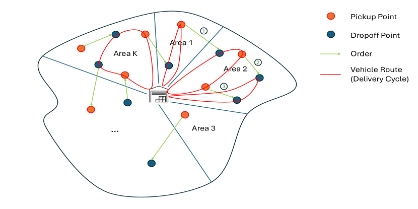
Figure 1: Illustration of meal delivery through a microhub

Consider a meal delivery service offered in an isotropic region of area $A$, with an average order arrival flux $\lambda$ (i.e., order arrivals per hour per square mile), a total number of deliverers $m$, and a microhub placed inside. As shown in Figure 1, the region is further divided into $K$ sub-areas, and each sub-area $k\in K$ comes with a coverage of $A_{k}$, order arrival rate $\lambda_{k}(=\lambda A_{k})$, and $m_{k}$ dedicated deliverers. The objective is to determine the optimal partitioning strategy that defines $A_{k}^{*}$ and $m_{k}^{*}$ as constrained by $\sum_{k}m_{k}^{*}=m$ and $\sum_{k}A_{k}^{*}=A$. Given the partition of sub-areas, individual delivery orders could be categorized as either intra-zonal (both pickup and drop-off locations within the same sub-area) or inter-zonal (pickup and drop-off locations in different sub-areas).

Delivery vehicles are dispatched to manage pickup and drop-off tasks within their assigned areas, with each vehicle designated to serve only one specific sub-area. During one delivery cycle, which refers to a round trip starting and ending at the microhub, vehicles conduct both pickup and drop-off tasks. For each order, one delivery cycle can only visit either its pickup point or drop-off point. The delivery vehicles are dispatched once there are $n_{k}$ nodes accumulated in each area $k$ to visit. These $n_{k}$ nodes comprise both the meals waiting for drop-off at the microhub and the meals awaiting pickup at the restaurants. Thus, meal delivery operates under two situations:

• For an intra-zonal order, one deliverer picks up the meal package from the restaurant during the first available delivery cycle and transfers it back to the microhub. Later, either the same deliverer or another one picks up the package from the microhub and drops it off during a subsequent delivery cycle. For example, in Figure 1, Orders 2 and 3 in Area 2 are initially picked up by one deliverer and dropped off during a later delivery cycle.

• For an inter-zonal order, a deliverer first picks up the meal and transfers it to the microhub. Then, another deliverer, which serves the area where the order’s drop-off point is located, retrieves the package from the microhub and delivers it to its destination. For example, in Figure 1, Order 1 is picked up by a deliverer servicing Area 1, transferred to the microhub, and then dropped off by another deliverer servicing Area 2. When the deliverer drops off the package in Area 2, they might also batch it with other pickup tasks for Orders 2 and 3 during the same delivery cycle to ensure efficient service.

Thus, for each delivery epoch, this delivery pattern closely resembles the one-to-many-to-one (1-M-1) pickup and delivery problem, which involves two distinct sets of commodities: some are shipped from the microhub to the customers, and others are picked up at the restaurants and returned to the microhub Toth and Vigo, (2002).

3.2 Lifetime of meal delivery orders

Based on the above design of microhub, one meal order’s lifetime can be divided into the following four parts according to Figure 2:

• Meal preparation time: Interval from when an order is placed until it is ready for pickup;

• Pickup time: Interval from the meal package being ready to its delivery at the microhub;

• Transfer time: Interval that the package is held at the microhub for the next delivery cycle;

• Drop-off time: Interval for transporting the package from the microhub to the customer.

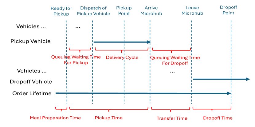
Figure 2: Lifetime of individual meal delivery orders

Among these four parts, the meal preparation time is unaffected by the introduction of the microhub and will therefore be left out in the following analysis. The pickup time can be further broken down into three phases: the period from when the package is ready for pickup until a deliverer is dispatched, the interval between the dispatch of the deliverer and the actual pickup of the order, and the time required for the package to be transported from the restaurant to the microhub. The combined duration of the latter two phases indeed constitutes one complete delivery cycle to a deliverer. Additionally, it should be noted that when a meal is ready for pickup, it does not guarantee the immediate dispatch of a deliverer. Two conditions must be satisfied:

• The first condition is to accumulate $n_{k}$ nodes to visit within its pickup sub-area.

• Once $n_{k}$ nodes are accumulated, it still needs to wait for a deliverer to take care of the batch service if none of the deliverers serving this sub-area $k$ are available immediately.

This waiting time for pickup, along with the transfer time (which can also be considered the waiting time for drop-off), can be modeled using a queuing network with $K$ dependent queues. The detailed modeling of the queuing network and the derivation of the average waiting time will be discussed later.

3.3 Approximation of traveling salesman tours

Before diving deep into the queuing network, we first analyze the expectation and variance of individual deliverers’ traveling distances during a single delivery cycle. These distances will determine the service rate for each queue that represents a specific sub-area. For each delivery cycle, the deliverer tours inside a sub-area following a TSP. According to (Daganzo, 1984b, ), the optimal approximation of the TSP can be achieved by dividing each zone into several long strips of width $w$. Let $X$ denote the random distance between two consecutive nodes along the width of the strip, $Y$ as the one along the side of the strip, and $\delta$ as the density of nodes to visit per unit area per hour. For the $L_{1}$ distance metric setting, $d_{w}$ is the traveling distance for two consecutive nodes within each swath, its mean can be derived as:

$$d_{w} =X+Y,$$

$$\mathop{{}\mathbb{E}}[d_{w}] =\mathop{{}\mathbb{E}}[X]+\mathop{{}\mathbb{E}}[Y]=\frac{w}{3}+\frac{1}{\delta w}.$$

If there are $N$ nodes to visit in one delivery cycle, to minimize the total expected tour length $N\cdot\mathop{{}\mathbb{E}}[d_{w}]$ traveled by one vehicle, (Daganzo, 1984b, ) obtained the optimal swath length of $w^{*}=\sqrt{3/\delta}$ and since $N=\delta A$, the expectation of the approximated optimal TSP solution can be expressed as:

$$\mathop{{}\mathbb{E}}[N\cdot d_{w}^{*}]=\mathop{{}\mathbb{E}}(A,N)=\frac{2}{\sqrt{3}}\sqrt{AN}.$$

If we follow the same swath partition rule, we will obtain the following variance of the TSP distance:

$$\mathop{{}\mathrm{Var}}[N\cdot d_{w}^{*}]=\mathop{{}\mathrm{Var}}(A,N) =N^{2}\left(\mathop{{}\mathrm{Var}}[X]+\mathop{{}\mathrm{Var}}[Y]+2Cov(X,Y)\right)$$

$$=N^{2}\left(\frac{w^{*2}}{18}+\frac{1}{(\delta w^{*})^{2}}\right)$$

$$=\frac{AN}{2}.$$

However, such a derivation significantly overestimates the ground-truth variance.

In general, for the case of fewer points to visit, their spatial dispersion could be highly uncertain, either concentrating in specific areas or spreading over the entire region. Conversely, as the number of points to visit increases, they tend to spread more evenly across the region. We infer that the variance of the TSP shall characterize the following properties:

• $\mathop{{}\mathrm{Var}}(A,N)$ is proportional to $A$;

• $\mathop{{}\mathrm{Var}}(A,N)$ is inversely proportional to $N$;

• When $N$ approaches infinity, $\mathop{{}\mathrm{Var}}(A,N)$ converges to a strictly positive level.

Based on the above deduction, we propose the following hypothetical form for describing the variance of travel distances under the TSP:

$$\mathop{{}\mathrm{Var}}(A,N)=C\cdot A\cdot\left(\frac{\gamma}{N^{\alpha}}+\beta\right).$$

The hyperparameters $C,\gamma,\alpha,\beta$ will be calibrated later through simulation, with the effectiveness of the proposed approximation also demonstrated then.

Let $D_{k}$ and $S_{k}$ denote the travel distance and time spent by individual deliverers for completing one delivery cycle in sub-area $k$, respectively. As a summary, their expectations and variances under the TSP can be obtained as follows:

$$\mathop{{}\mathbb{E}}[D_{k}] =\frac{2}{\sqrt{3}}\sqrt{A_{k}n_{k}},$$ (1)

$$\mathop{{}\mathrm{Var}}[D_{k}] =C\cdot A_{k}\cdot\left(\frac{\gamma}{n_{k}^{\alpha}}+\beta\right),$$ (2)

$$\mathop{{}\mathbb{E}}[S_{k}] =\mathop{{}\mathbb{E}}[\frac{D_{k}}{v}]=\frac{2}{v\sqrt{3}}\sqrt{A_{k}n_{k}},$$ (3)

$$\mathop{{}\mathrm{Var}}[S_{k}] =\mathop{{}\mathrm{Var}}[\frac{D_{k}}{v}]=\frac{C\cdot A_{k}}{v^{2}}\cdot\left(\frac{\gamma}{n_{k}^{\alpha}}+\beta\right),$$ (4)

where $v$ denotes the speed of delivery vehicles.

3.4 Queuing network analysis

The previous section derives, from the perspective of a deliverer, the expected traveling distance of one delivery cycle, which will be employed as the service rate to analyze meal packages’ waiting time for pickup and transfer. Both waiting times can be modeled using the following Jackson queuing network as shown in Figure 3. For the $K$ sub-areas that divide the service region, each sub-area can be treated as a queue with its own servers. Additionally, the following assumptions are made for this queuing network:

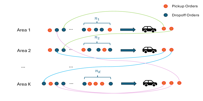
Figure 3: Cross-zonal meal delivery process as a queuing network

• The network has $K$ single-station queues.

• For each queue, when there is an idle deliverer and the number of orders in the queue is $n_{k}$ or more, a batch of exactly $n_{k}$ orders is taken for service.

• The $k$th area has $m_{k}$ vehicles for delivery. The number of vehicles $m_{k}$ in each area is a decision variable determined by the aggregate system optimization.

• New orders arrive at sub-area $k$ in Poisson with an arrival rate of $\lambda_{k}$.

• Service times for meal packages at sub-area $k$ are i.i.d., with a mean $\mathop{{}\mathbb{E}}[S_{k}]$ and a variance $\mathop{{}\mathrm{Var}}[S_{k}]$.

• A package picked up from sub-area $i$, after being transferred to the microhub, will join the queue at sub-area $k$ for drop-off with probability $p_{i,k}$. Suppose the destinations are uniformly distributed over the space, then $p_{i,k}=A_{k}/A$. Once a package is dropped off, it exits the queuing network completely.

• There are unlimited waiting spots at each queue, indicating that the microhub is sufficiently large to accommodate all incoming packages.

For an arbitrary order, the first step is to wait until $n_{k}$ orders—either pickup or drop-off—accumulate for batch service. This process can be viewed as a classical Poisson process with an arrival rate $\delta_{k}$, which is determined by the summation of new arriving orders in sub-area $k$ for pickup and the collected orders from all sub-areas that need to be dropped off to sub-area $k$, i.e.,

$$\delta_{k}=\lambda_{k}+\sum_{i=1}^{K}\lambda_{i}p_{i,k}.$$ (5)

Let $W_{i}$ denote the waiting time of the $i$-th order arrived before reaching the $n_{k}$ threshold as a single batch. Then, for the $i$-th order, its waiting time would be $W_{i}=(n_{k}-i)/\delta_{k}$. Thus, for an arbitrary order, we can derive the average waiting time $W_{a}$ until accumulating $n_{k}$ orders as follows:

$$W_{k}^{a} =\frac{1}{n_{k}}\sum_{i=1}^{n_{k}}\frac{n_{k}-i}{\delta_{k}}=\frac{n_{k}-1}{2\delta_{k}}.$$ (6)

After collecting $n_{k}$ points to visit, the next step is to calculate the waiting time for the next available deliverer for processing the batched orders. For each sub-area, this process of forming delivery cycles can be modeled through a $G/G/m$ queue. The time interval between the arrivals of consecutive service batches follows an Erlang distribution with the shape parameter $n_{k}$ and the rate parameter $\delta_{k}$. The service rate of a deliverer in fulfilling one delivery cycle is determined by the travel time for a TSP tour described previously. The number of servers for each queue is $m_{k}$. Since the Erlang distribution is non-memoryless, there is no analytical solution for the waiting time in this $G/G/m$ queue. Here, we use the widely applicable approximation for the average waiting time in a $G/G/m$ queue Larson and Odoni, (1981), presented as follows,

$$W_{k}^{q}\approx\frac{\left[\frac{n_{k}}{\delta_{k}^{2}}+\frac{1}{m_{k}}\mathop{{}\mathrm{Var}}[S_{k}]\right]\cdot\frac{\delta_{k}}{n_{k}}}{2\left(1-\frac{\delta_{k}\cdot\mathop{{}\mathbb{E}}[S_{k}]}{n_{k}\cdot m_{k}}\right)}.$$ (7)

4 Optimal design problem

The design problem aims to determine the optimal zonal partition, batch size, and number of deliverers for each sub-area, given the order arrival flux $\lambda$ and the total number of deliverers in shift $m$. Since the amortized fixed cost and operational cost of the microhub cannot be optimized through the partition strategy, they will not be considered in this analysis. Accordingly, the total system cost will consist of two aspects: the vehicle miles traveled by deliverers and the customers’ waiting time.

4.1 Vehicle miles traveled $Q$

For each sub-area, when $n_{k}$ orders are collected, one deliverer is dispatched to visit these $n_{k}$ points, while other idle deliverers if any wait near the microhub waiting for the next delivery. Thus, the expected vehicle miles traveled per hour by all deliverers in sub-area $k$, denoted as $Q_{k}$, is given by the product of the number of delivery cycles per hour and the expected traveling distance for visiting $n_{k}$ points. Specifically,

$$Q_{k} =\frac{\delta_{k}}{n_{k}}\cdot\mathop{{}\mathbb{E}}[D_{k}]=2\delta_{k}\sqrt{\frac{A_{k}}{3n_{k}}}.$$ (8)

4.2 Customer’s waiting time $W$

For meal delivery, one of the most critical metrics for customer satisfactory is the waiting time for package delivery. As previously noted, each customer’s waiting time can be divided into four components, with the meal preparation time excluded from this analysis. The waiting time for package pickup and transfer can be expressed as $W_{k}^{a}+W_{k}^{q}$. The drop-off time can be viewed as the time from the dispatch of one deliverer until the package is delivered during a delivery cycle.

According to (Larson and Odoni,, 1981), the mean time $V$ from the occurrence of one event until a random incidence depends on the mean and variance of the inter-event time $I$ as follows:

$$\mathop{{}\mathbb{E}}[V]=\frac{\mathop{{}\mathrm{Var}}[I]+\mathop{{}\mathbb{E}}^{2}[I]}{2\mathop{{}\mathbb{E}}[I]}.$$

Combining all these components, the expected total waiting time for an arbitrary meal delivery, $W_{k}$, can be expressed as:

$$W_{k} =W_{k}^{a}+W_{k}^{q}+\mathop{{}\mathbb{E}}[S_{k}]+W_{k}^{a}+W_{k}^{q}+\frac{\mathop{{}\mathrm{Var}}[S_{k}]+\mathop{{}\mathbb{E}}^{2}[S_{k}]}{2\mathop{{}\mathbb{E}}[S_{k}]},$$ (9)

where $W_{k}^{a}+W_{k}^{q}+\mathop{{}\mathbb{E}}[S_{k}]$ accounts for the pickup time, $W_{k}^{a}+W_{k}^{q}$ represents the transfer time, and the last term in Eq. (9) stands for the drop-off time.

4.3 Formulation

The optimal system design then solves the following optimization problem:

$$\min_{\{\lambda_{k},A_{k},n_{k},m_{k}\}}\sum_{k=1}^{K}\left(\pi_{Q}\cdot Q_{k}+\pi_{W}\cdot\lambda_{k}W_{k}\right)$$ (10a)

s.t. $$(\ref{eq_E_Dk})-(\ref{eq_waiting_time})$$

$$A=\sum_{k=1}^{K}A_{k}$$ (10b)

$$m=\sum_{k=1}^{K}m_{k}$$ (10c)

$$\lambda_{k}=\lambda A_{k} \forall k=1,2,3,\dots$$ (10d)

$$p_{i,k}=\frac{A_{k}}{A} \forall i,k=1,2,3,\dots$$ (10e)

$$\delta_{k}\leq\frac{m_{k}}{\mathop{{}\mathbb{E}}[S_{k}]/n_{k}} \forall k=1,2,3,\dots$$ (10f)

$$A_{k},n_{k},m_{k}\geq 0 \forall k=1,2,3,\dots$$ (10g)

The objective (10b) represents the generalized total cost of the meal delivery system, encompassing both the operational costs of deliverers and the time costs incurred by customers; Constraints (10b) and (10c) ensure that the total area and the total number of vehicles allocated to each sub-area match the overall area and total number of vehicles for the entire region, respectively; Constraint (10d) stipulates that the order generation rate in each sub-area is proportional to its area; Constraint (10e) specifies the probability of any pickup order originated from sub-area $i$ having its drop-off destination in sub-area $k$ based on the area size of sub-area $k$; finally, Constraint (10f) ensures that the queuing system in each sub-area remains in steady states.

5 Numerical analysis

The optimal design problem of the proposed system with a microhub is evaluated through a series of simulation experiments. First, we provide a brief comparison between the approximation model and the simulated results to demonstrate the accuracy of our predicted travel distance and customer waiting time. Next, we conduct a comprehensive evaluation of the performance of our proposed design and compared it to the strategy without the microhub under various market conditions.

5.1 Experimental setup

In this experiment, we consider an ideal isotropic square area $A$ and use an equal partition strategy to divide the entire area and the supply of deliverers evenly into $K$ sub-areas. With this, we can simplify the relationships for any sub-area $k\in K$ as follows,

$$n_{k} =n,$$ (11)

$$A_{k} =\frac{A}{K},$$ (12)

$$\lambda_{k} =\lambda\frac{A}{K},$$ (13)

$$m_{k} =\frac{m}{K}.$$ (14)

Besides, we assume that the pickup and drop-off locations of each meal delivery order are uniformly distributed across the entire area. Therefore,

$$p_{i,k}=\frac{1}{K},$$

which further simplifies the order arrival for batch services $\delta_{k}$ as follows:

$$\delta_{k} =\lambda_{k}+\sum_{i=1}^{K}\lambda_{i}\cdot\frac{1}{K}=2\lambda_{k}.$$ (15)

The optimal design problem now reads:

$$\min_{n,K}\ K\cdot\left(\pi_{Q}\cdot Q_{k}+\pi_{W}\cdot\lambda_{k}W_{k}\right)$$ (16a)

s.t. $$\eqref{eq_E_Dk}-\eqref{eq_waiting_time},\ \eqref{eq_variables_simplified_lambda}-\eqref{eq_variables_simplified_delta}$$

$$\delta_{k}\leq\frac{m_{k}}{\mathop{{}\mathbb{E}}[S_{k}]/n_{k}} \forall k=1,\dots,K$$ (16b)

$$A_{k},n_{k},m_{k}\geq 0 \forall k=1,\dots,K$$ (16c)

The optimal design in this case is determined by two decisions related to the number of orders to batch $n$, and the number of sub-areas $K$. These decisions are made given the exogenous inputs, which include the order arrival flux $\lambda$, the coverage area $A$, and the fleet size $m$.

5.2 Simulation and measurement

Simulations are conducted to demonstrate the effectiveness of proposed approximations for TSP tours—Eqs. (3), (4)—and for customer waiting time—Eqs. (6), (7), (9). The simulated results are compared against the predicted approximation for a set of scenarios with different values for $\{\lambda,A,m,n,K\}$ to measure the approximation accuracy. The vehicular speed is set as 40 mph in the numerical analysis.

Measurement of approximations for TSP

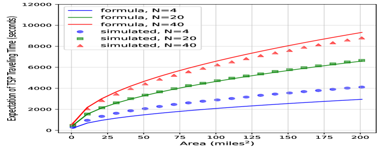
(a)

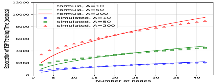
(b)

Figure 4: Comparison between measured and predicted expectation of the traveling time through TSP tours w.r.t. (a) area size and (b) number of nodes.

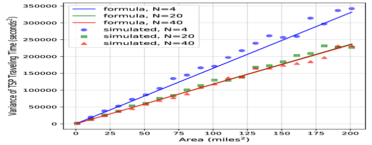
(a)

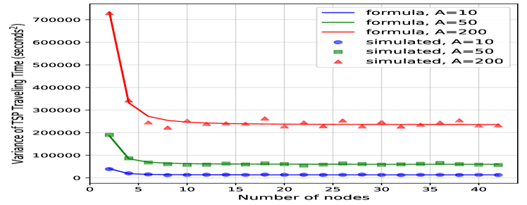
(b)

Figure 5: Comparison between measured and predicted variance of the traveling time through TSP tours w.r.t. (a) area size and (b) number of nodes.

We vary the values of $A$ and $N$ and simulate 1,000 trips for each case, where $N$ nodes are randomly distributed across a square area of $A$. The simulated results are obtained through the built-in solvers provided by Google OR-Tool’s vehicle routing package, and we then calculate the average and variance of travel time across the 1,000 simulations for each point given $A$ and $N$. For $\mathop{{}\mathrm{Var}}(A,N)$, we calibrate Eq. (4) using the simulation results, and obtain $C^{*}=27.49$, $\gamma^{*}=465.40$, $\alpha^{*}=2.37$, and $\beta^{*}=45.57$. Figures 4 and 5 display the fitting curves for the expectation and variance of the traveling time through TSP tours. The results show that the approximations using Eqs. (3) and (4) achieve $R^{2}$ values of 96.27% and 99.28%, respectively, compared to the optimal solutions provided by Google OR-Tool.

Measurement of approximations for customer waiting time

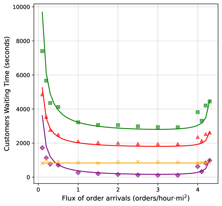
(a)

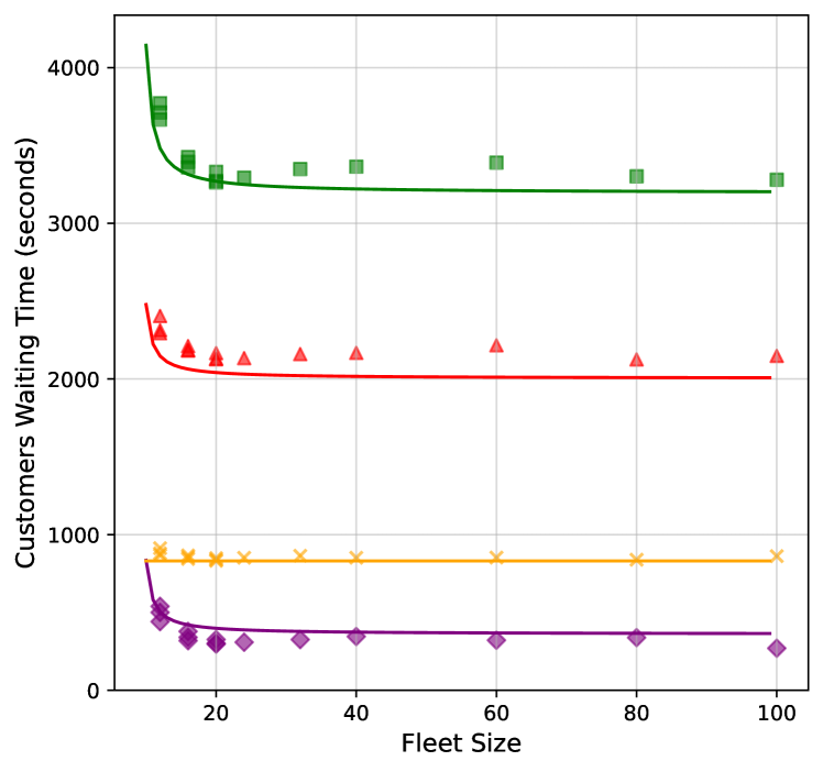
(b)

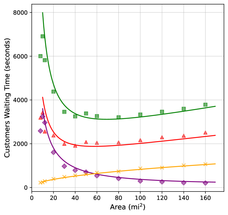
(c)

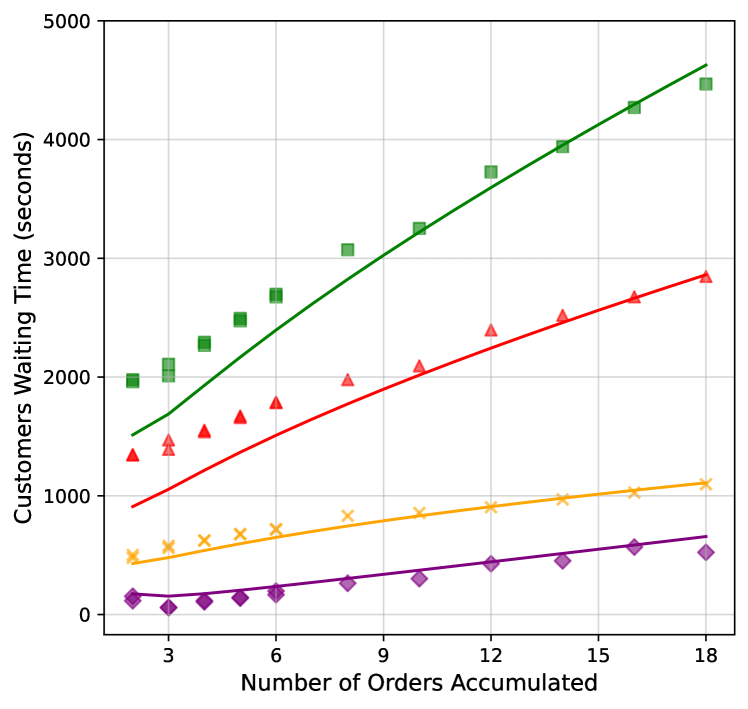
(d)

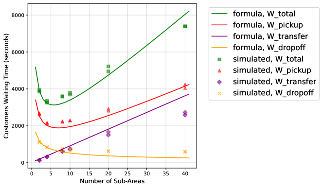
(e)

Figure 6: Comparison between measured and predicted variance of the traveling time through TSP tours w.r.t. (a) order arrival flux, (b) fleet size; (c) area, (d) batch size of orders, (e) number of sub-area partitions.

The “ground truth” arrivals of delivery requests and customers’ waiting time are simulated over a 6-hour period to experiment with the order fulfillment process. The arrival of requests follows a spatio-temporal Poisson distribution with a given $\lambda$. Once a sub-area accumulates $n$ orders and there is a deliverer available, one deliverer is dispatched to visit the $n$ nodes following the routing provided by the Google OR-Tool. The simulation platform records the critical time points for each order, including the total waiting time from its generation to its delivery (“W_total” in Figure 6), as well as the three decomposed components described in Section 3.2. The first hour is excluded as a warm-up period, and the average waiting time of all orders is calculated over the remaining five hours. The baseline parameters are set as follows: order arrival flux $\lambda=1$ (1/hour$\cdot$mi²), fleet size $m=40$, area $A=100$ (mi²), $n=10$ orders to accumulate, and $K=4$ sub-areas partitioned. For each plot in Figure 6, four out of the five parameters are held constant, while the total and three decomposed components of customer waiting time are plotted with respect to the varying parameter.

As shown in Figure 6a, when the order arrival rate is too low, it takes a long time to accumulate $n$ orders for batch service, resulting in devastating wait for customers. Conversely, when the arrival rate is high and exceeds the service capacity of the given fleet size, the system becomes congested, thereby leading to increased waiting time as well. Similarly, Figure 6b illustrates that a shortage of deliverers leads to a more congested system. However, once there is sufficient capacity, adding more deliverers does not yield noticeable improvements, as many will remain idle. In a trend similar to the arrival rate, Figure 6c shows that if the service area is too small, it is difficult to accumulate $n$ orders. Conversely, for a large area, the total waiting time increases due to the longer travel time needed per delivery cycle.

Interestingly, Figure 6d evidences that a higher $n$ consistently leads to a longer waiting time for accumulating $n$ orders. However, as demonstrated in Eq. (16a), batching more orders per delivery tour reduces vehicle miles traveled. Meanwhile, for different numbers of partitioned sub-areas, Eqs. (6) and (7) indicate that a more granular partition of sub-areas results in a longer time for accumulating $n$ nodes to visit, but a shorter traveling distance within each sub-area. Consequently, the trend of the total waiting time is non-monotonic, as displayed in Figure 6e. These trade-offs over the choices of $n$ and $K$ justify the existence of optimal system designs with moderate setups rather than extreme values.

5.3 Effectiveness of the microhub

We then proceed to evaluate the effectiveness of the proposed transshipment of meal packages by comparing the total vehicle miles traveled and customer waiting time with those achieved using a heuristic TSPPD approximation proposed by (Daganzo,, 1978). In this strategy, deliverers are routed to the nearest point pending a visit, which can be either an origin of a pickup order or a destination of an drop-off order on the vehicle. At equilibrium, the number of nodes waiting ($N_{w}$) should equal the number of packages en-route on delivery vehicles ($N_{v}$), and the arrival rate ($\lambda A$) equals the total service rate ($\mu m$), i.e.,

$$N_{w} =N_{v}$$ (17)

$$\lambda A =\mu m.$$ (18)

The service rate $\mu$ provided by individual deliverer equals

$$\mu =\left(\frac{2d_{N_{w}+N_{v}}}{v}\right)^{-1},$$ (19)

where $d_{N_{w}+N_{v}}$ is the distance to the nearest node when there are $N_{w}+N_{v}$ nodes to visit in this area. As derived previously, $d_{N_{w}+N_{v}}=\frac{2}{\sqrt{3}}\sqrt{\frac{A}{N_{w}+N_{v}}}$. By solving this along with Eqs. (17), (18), and (19), we determine the optimal number of packages to keep on the vehicles:

$$N_{v}^{*}=N_{w}^{*}=\frac{8\lambda^{2}A^{3}}{3m^{2}v^{2}}$$ (20)

Thus, the total waiting time for each customer, including the waiting time for package pickup and the riding time on a vehicle, equals:

$$W_{TSPPD} =\frac{N_{v}^{*}}{\lambda A}+\frac{N_{w}^{*}}{\mu}=\frac{N_{v}^{*}}{\lambda A}(m+1)$$ (21)

Similar to Eq. (8), the total vehicle miles traveled is given by the product of the number of visiting nodes generated per hour and the expected distance between the two adjacent visits:

$$Q_{TSPPD} =2\lambda A\cdot d_{2N_{v}^{*}}.$$ (22)

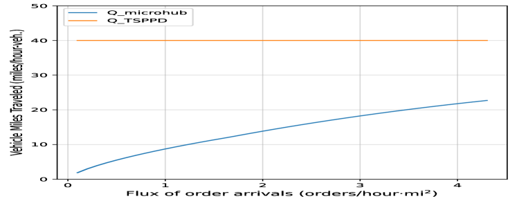
(a)

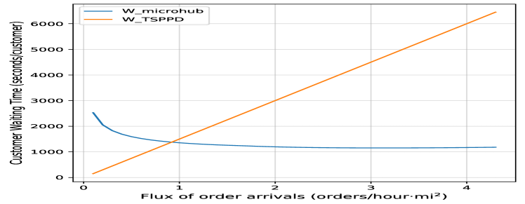
(b)

Figure 7: Comparison between the transshipment and non-transshipment strategies on (a) vehicle miles traveled and (b) customer waiting time w.r.t. order arrival flux.

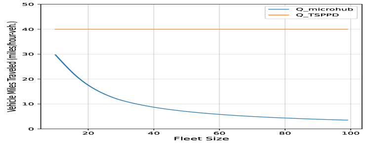
(a)

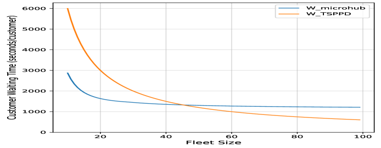
(b)

Figure 8: Comparison between the transshipment and non-transshipment strategies on (a) vehicle miles traveled and (b) customer waiting time w.r.t. delivery fleet size.

Adhering to the values suggested by (Nourbakhsh and Ouyang,, 2012), we set the operation cost per vehicle mile to $\pi_{Q}=\$2$/veh-mile, and customers’ time value to $\pi_{W}=\$20$/hour. We consider two scenarios in a 10$\times$10 square-mile area, varying either the order arrival flux or delivery fleet size, to evaluate the performance of the transshipment system compared to the non-transshipment TSPPD benchmark. In the first scenario, illustrated in Figure 7, the fleet size is held constant at 40 vehicles, while the order arrival flux varies from 0.1 to 4.3 orders/hour$\cdot$mi². In the second scenario, shown in Figure 8, the order arrival flux is set at $\lambda=1$, and the fleet size ranges from 10 to 100 vehicles. For both scenarios, given the area $A$, fleet size $m$, and order arrival flux $\lambda$, we solve the optimization problem (16) to determine the optimal partition $K$ and the batch size $n$. We then compute the average customer waiting time “W_microhub” (seconds/customer) and the average vehicle miles traveled “Q_microhub” (miles/hour-vehicle). Concurrently, we use Eqs. (22) and (21) to calculate “W_TSPPD” and “Q_TSPPD” for the TSPPD benchmark.

The comparisons in Figures 7 and 8 highlight the conditions under which transshipment demonstrates relative strength compared to non-transshipment strategies. From Figures 7a and 8a, it is evident that under the transshipping strategy through a mirohub, the average vehicle miles traveled decreases as the arrival rate drops or the fleet size increases. In contrast, the TSPPD benchmark maintains a constant vehicle miles travelled at 40 miles/hour-vehicle. This constancy occurs because, in (Daganzo,, 1978)’s strategy, there are always pending orders to take by deliverers, they are continually traverse to the next visit points without breaks. But in our design, when the cumulative number of nodes to visit is below $n$, deliverers wait at the microhub for the next delivery cycle, thereby consistently saving distances compared to the TSPPD benchmark. Furthermore, in Figure 7b, the transshipment strategy demonstrates a reduction in customer waiting time as demand increases within the examined regime, contrasting with the TSPPD benchmark. This indicates that, with adequate service capacity, system efficiency can possibly improve as demand rises by optimizing the number of sub-areas and the batching size of orders. At lower demand levels, however, the transshipment through the microhub becomes less efficient than the direct pickup and delivery strategy due to the additional time required for routing and transferring. Similarly, Figure 8b shows that transshipment is advantageous in congested systems with fewer vehicles by batching orders together for service. However, with a sufficient fleet size, the TSPPD strategy outperforms the transshipment through the microhub. In summary, transshipment through a microhub provides benefits over non-transshipment strategies in scenarios with high demand or insufficient supply.

6 Conclusion

This paper proposes a new meal delivery strategy integrating a microhub. The microhub serves as a temporary storage and transfer point for meals between different sub-areas of service. An analytical model was developed using a CA method to evaluate the system’s expected performance. To estimate customer waiting time, we decomposed the lifecycle of a meal order and adapted a queuing network to approximate the transfer time at the microhub. A comprehensive set of simulations was conducted to validate the accuracy of these approximations. The analytical approximations were then incorporated into an optimal design problem to solve for the optimal system design, specifically related to the number of sub-areas and the batch size for orders. The numerical results indicate that with the system optimally configured, the proposed meal delivery strategy through transshipment significantly reduces vehicle miles traveled compared to a traditional VRPPD strategy without transshipment. Additionally, the transshipment strategy also decreases expected customer waiting time effectively under high demand or low supply conditions. However, in scenarios with sufficient supply, excessive transshipment might cause longer wait for customers.

Future research can explore several promising directions. (i) This paper examines the simplest scenario with a single microhub serving an isotropic area. Future research could extend this to scenarios involving multiple microhubs optimally positioned within a larger area. In such cases, a two-echelon operations can be investigated, with micromobilities such as e-bikes or e-scooters serving smaller areas covered by individual microhubs and larger delivery vehicles periodically transporting between microhubs. (ii) The variance of traveling distances for TSP tours was formulated based on deductions. Further research is needed to investigate the physical justification for the hypothetical model and understand the underlying mechanics. (iii) The current simulation experiments demonstrated strong predictive ability for our model on the idealized setting considered in this paper. The resulting performance comparisons with VRPPD and other findings would benefit from further verification in more noisy environments, ideally using real-world data. (iv) Finally, it would be meaningful to endogenize customer demand and deliverer supply. The former will be dependent on the realized customer waiting time, while deliverers’ entry decisions could be influenced by the rate of order completions and associated travel distances.

Nomenclature

Table 1: Notation list of parameters and variables

Notation	Description	Unit
Input Parameters
$\lambda$	Expected number of orders generated per hour per unit area	1/hour$\cdot$mi2
$m$	Total size of delivery fleet
$v$	Speed of delivery vehicles	mph
$A$	Total area of the region	mi2
$C,\gamma,\alpha,\beta$	Parameters related to the variance of TSP distances
$\pi_{Q}$	Operating cost per vehicle mile travelled	$
$\pi_{W}$	Value of time	$/hour
Decision Variables
$K$	Number of sub-area partitions
$A_{k}$	Area of each sub-area $k$	mi2
$\lambda_{k}$	Expected number of new orders generated per hour in sub-area $k$	1/hour
$\delta_{k}$	Number of pickup and drop-off locations to visit in sub-area $k$	1/hour
$p_{i,k}$	Probability of an order picked up in sub-area $i$ being dropped off in $k$
$m_{k}$	Number of deliverers assigned to sub-area $k$
$n_{k}$	Number of packages accumulations in sub-area $k$ per delivery cycle
$D_{k}$	Traveling distance of individual deliverer in sub-area $k$ per delivery cycle	mi
$S_{k}$	Traveling time of individual deliverer in sub-area $k$ per delivery cycle	hour
$Q$	Expected total vehicle miles traveled per hour of operation	mph
$W_{a}^{k}$	Average waiting time for accumulating $n_{k}$ packages in sub-area $k$	hour
$W_{q}^{k}$	Average package holding time for available deliverers in sub-area $k$	hour
$W$	Average total waiting time per customer	hour

References

- Agatz et al., (2024) Agatz, N., Cho, S.-H., Sun, H., and Wang, H. (2024). Transportation-enabled services: Concept, framework, and research opportunities. Service Science, 16(1):1–21.
- Ansari et al., (2018) Ansari, S., Başdere, M., Li, X., Ouyang, Y., and Smilowitz, K. (2018). Advancements in continuous approximation models for logistics and transportation systems: 1996–2016. Transportation Research Part B: Methodological, 107:229–252.
- Campbell, (2013) Campbell, J. F. (2013). A continuous approximation model for time definite many-to-many transportation. Transportation Research Part B: Methodological, 54:100–112.
- (4) Chen, P. W. and Nie, Y. M. (2017a). Analysis of an idealized system of demand adaptive paired-line hybrid transit. Transportation Research Part B: Methodological, 102:38–54.
- (5) Chen, P. W. and Nie, Y. M. (2017b). Connecting e-hailing to mass transit platform: Analysis of relative spatial position. Transportation Research Part C: Emerging Technologies, 77:444–461.
- Chen et al., (2012) Chen, Q., Lin, J., and Kawamura, K. (2012). Comparison of urban cooperative delivery and direct delivery strategies. Transportation research record, 2288(1):28–39.
- Daganzo, (2005) Daganzo, C. (2005). Logistics systems analysis. Springer Science & Business Media.
- (8) Daganzo, C. and Newell, G. (1986a). Design of multiple-vehicle delivery tours–i: a ring-radial network. Transportation Research Part B, pages 345–364.
- Daganzo, (1978) Daganzo, C. F. (1978). An approximate analytic model of many-to-many demand responsive transportation systems. Transportation Research, 12(5):325–333.
- (10) Daganzo, C. F. (1984a). The distance traveled to visit n points with a maximum of c stops per vehicle: An analytic model and an application. Transportation science, 18(4):331–350.
- (11) Daganzo, C. F. (1984b). The length of tours in zones of different shapes. Transportation Research Part B: Methodological, 18(2):135–145.
- (12) Daganzo, C. F. (1987a). The break-bulk role of terminals in many-to-many logistic networks. Operations Research, 35(4):543–555.
- (13) Daganzo, C. F. (1987b). Increasing model precision can reduce accuracy. Transportation Science, 21(2):100–105.
- Daganzo et al., (2012) Daganzo, C. F., Gayah, V. V., and Gonzales, E. J. (2012). The potential of parsimonious models for understanding large scale transportation systems and answering big picture questions. EURO Journal on Transportation and Logistics, 1(1-2):47–65.
- (15) Daganzo, C. F. and Newell, G. F. (1986b). Configuration of physical distribution networks. Networks, 16(2):113–132.
- del Castillo, (1999) del Castillo, J. M. (1999). A heuristic for the traveling salesman problem based on a continuous approximation. Transportation Research Part B: Methodological, 33(2):123–152.
- Flushberg Sr and Wilson, (1976) Flushberg Sr, M. and Wilson, N. H. (1976). A descriptive supply model for demand-responsive transportation system planning.
- Ghaffarinasab et al., (2018) Ghaffarinasab, N., Van Woensel, T., and Minner, S. (2018). A continuous approximation approach to the planar hub location-routing problem: Modeling and solution algorithms. Computers & Operations Research, 100:140–154.
- Gunes et al., (2024) Gunes, S., Fried, T., and Goodchild, A. (2024). Seattle microhub delivery pilot: Evaluating emission impacts and stakeholder engagement. Case Studies on Transport Policy, 15:101119.
- Kaczmarski, (2024) Kaczmarski, M. (2024). Which company is winning the restaurant food delivery war? https://secondmeasure.com/datapoints/food-delivery-services-grubhub-uber-eats-doordash-postmates/.
- Kawamura and Lu, (2007) Kawamura, K. and Lu, Y. (2007). Evaluation of delivery consolidation in us urban areas with logistics cost analysis. Transportation research record, 2008(1):34–42.
- Kohar and Jakhar, (2021) Kohar, A. and Jakhar, S. K. (2021). A capacitated multi pickup online food delivery problem with time windows: a branch-and-cut algorithm. Annals of Operations Research, pages 1–22.
- Larson and Odoni, (1981) Larson, R. C. and Odoni, A. R. (1981). Urban operations research. Number Monograph.
- Lin et al., (2016) Lin, J., Chen, Q., and Kawamura, K. (2016). Sustainability si: logistics cost and environmental impact analyses of urban delivery consolidation strategies. Networks and Spatial Economics, 16:227–253.
- Liu et al., (2021) Liu, S., He, L., and Max Shen, Z.-J. (2021). On-time last-mile delivery: Order assignment with travel-time predictors. Management Science, 67(7):4095–4119.
- Liu, (2019) Liu, Y. (2019). An optimization-driven dynamic vehicle routing algorithm for on-demand meal delivery using drones. Computers & Operations Research, 111:1–20.
- Marcucci and Danielis, (2008) Marcucci, E. and Danielis, R. (2008). The potential demand for a urban freight consolidation centre. Transportation, 35:269–284.
- Naseraldin and Herer, (2011) Naseraldin, H. and Herer, Y. T. (2011). A location-inventory model with lateral transshipments. Naval Research Logistics (NRL), 58(5):437–456.
- Newell, (1971) Newell, G. F. (1971). Dispatching policies for a transportation route. Transportation Science, 5(1):91–105.
- Newell and Daganzo, (1986) Newell, G. F. and Daganzo, C. F. (1986). Design of multiple vehicle delivery tours—ii other metrics. Transportation Research Part B: Methodological, 20(5):365–376.
- Nourbakhsh and Ouyang, (2012) Nourbakhsh, S. M. and Ouyang, Y. (2012). A structured flexible transit system for low demand areas. Transportation Research Part B: Methodological, 46(1):204–216.
- Ouyang and Yang, (2023) Ouyang, Y. and Yang, H. (2023). Measurement and mitigation of the “wild goose chase” phenomenon in taxi services. Transportation Research Part B: Methodological, 167:217–234.
- Pahwa and Jaller, (2022) Pahwa, A. and Jaller, M. (2022). A cost-based comparative analysis of different last-mile strategies for e-commerce delivery. Transportation Research Part E: Logistics and Transportation Review, 164:102783.
- Shi and Xu, (2024) Shi, L. and Xu, Z. (2024). Dine in or takeout? trends on restaurant service demand amid the covid-19 pandemic. Service Science.
- Shi et al., (2022) Shi, L., Xu, Z., Lejeune, M., and Luo, Q. (2022). An integer l-shaped method for dynamic order fulfillment in autonomous last-mile delivery with demand uncertainty. arXiv preprint arXiv:2208.09067.
- Simoni and Winkenbach, (2023) Simoni, M. D. and Winkenbach, M. (2023). Crowdsourced on-demand food delivery: An order batching and assignment algorithm. Transportation Research Part C: Emerging Technologies, 149:104055.
- Smilowitz and Daganzo, (2007) Smilowitz, K. R. and Daganzo, C. F. (2007). Continuum approximation techniques for the design of integrated package distribution systems. Networks: An International Journal, 50(3):183–196.
- Steever et al., (2019) Steever, Z., Karwan, M., and Murray, C. (2019). Dynamic courier routing for a food delivery service. Computers & Operations Research, 107:173–188.
- Stein, (1978) Stein, D. M. (1978). An asymptotic, probabilistic analysis of a routing problem. Mathematics of Operations Research, 3(2):89–101.
- Toth and Vigo, (2002) Toth, P. and Vigo, D. (2002). The vehicle routing problem. SIAM.
- Tsao et al., (2012) Tsao, Y.-C., Mangotra, D., Lu, J.-C., and Dong, M. (2012). A continuous approximation approach for the integrated facility-inventory allocation problem. European journal of operational research, 222(2):216–228.
- Wiles and van Brunt, (2001) Wiles, P. G. and van Brunt, B. (2001). Optimal location of transshipment depots. Transportation Research Part A: Policy and Practice, 35(8):745–771.
- Wilson et al., (1969) Wilson, N., Sussman, J., Goodman, L., and Higonnet, B. (1969). Simulation of a computer aided routing system (cars). Technical report, Institute of Electrical and Electronics Engineers (IEEE).
- Wilson et al., (1976) Wilson, N. H. M., Weissberg, R. W., and Hauser, J. (1976). Advanced dial-a-ride algorithms research project. Technical report.
- Xie and Ouyang, (2015) Xie, W. and Ouyang, Y. (2015). Optimal layout of transshipment facility locations on an infinite homogeneous plane. Transportation Research Part B: Methodological, 75:74–88.
- Xu et al., (2020) Xu, Z., Yin, Y., and Ye, J. (2020). On the supply curve of ride-hailing systems. Transportation Research Part B: Methodological, 132:29–43.