Multi-controlled single-qubit unitary gates based on the quantum Fourier transform

Abstract

Multi-controlled (MC) unitary (U) gates are widely employed in quantum algorithms and circuits. Few state-of-the-art decompositions of MCU gates use non-elementary $C-R_{x}$ and $C-U^{1/2^{m-1}}$ gates resulting in a linear function for the depths of an implemented circuit on the number of these gates. Our approach is based on two generalizations of the multi-controlled X (MCX) gate that uses the quantum Fourier transform (QFT) comprised of Hadamard and controlled-phase gates. For the native gate set used in a genuine quantum computer, the decomposition of the controlled-phase gate is twice as less complex as $C-R_{x}$, which can result in an approximately double advantage of circuits derived from the QFT. The first generalization of QFT-MCX is based on altering the controlled gates acting on the target qubit. These gates are the most complex and are also used in the state-of-the-art circuits. The second generalization relies on the ZYZ decomposition and uses only one extended QFT-based circuit to implement the two multi-controlled X gates needed for the decomposition. Since the complexities of this circuit are approximately equal to the QFT-based MCX, our MCU implementation is more advanced than any known existing. The supremacy over the best-known optimized algorithm will be demonstrated by comparing transpiled circuits assembled for execution in a genuine quantum device. One may note that our implementations use approximately half the number of elementary gates compared to the most efficient one, potentially resulting in a smaller error. Additionally, we elaborated optimization steps to simplify the state-of-the-art linear-depth decomposition (LDD) MCU circuit to one of our implementations.

MSC Classification]03G12, 81P68

1 Introduction

Current quantum devices are constrained by the number of qubits available and the noise introduced during the execution of nonideal quantum operations employing the native gates used for computation in a genuine quantum device. The hardware of these Noisy Intermediate-Scale Quantum devices (NISQ) [1] is constantly improving by increasing the number of qubits and fidelity of the native gates used in a particular quantum computing architecture. However, the efficiency in performing quantum computation can be improved by optimizing software that defines a quantum circuit implementation. It can be achieved by more efficient error mitigation [2], quantum state preparation [3, 4, 5], and decomposition of unitary gates into scalable quantum circuits in the basis set of elementary gates [6, 7, 8, 9]. The decomposition of a circuit is usually not unique. Therefore, different optimization techniques can be used to minimize the circuit’s depth and (or) the number of elementary gates used [10, 11, 12].

The first algorithm for decomposing multi-controlled $U(2)$ gates, which doesn’t use auxiliary qubits, was proposed in Ref. [6]. It exhibits a quadratic increase in the circuit depth and number of elementary gates with the number of control qubits. The authors showed that implemented circuits can be efficiently reduced by removing some gates at the price of phase relativization, using ancilla qubits, and approximating gates up to the target error $\epsilon$. The advantages of using relative-phase Toffoli gates to obtain linear depths of $n$-qubit MCX gates were first recognized in Ref. [13]. The effectiveness of this approach is demonstrated theoretically [14] and experimentally [15]. To correct phases, an additional $(C-R_{x})$-based circuit is introduced in Ref. [16] that approximately doubles the complexity of the previously simplified circuit. Different approximations are used to reduce the number of elementary gates in this circuit [17, 18]. As for all other cases, using auxiliary qubits lowers the circuit depth [19, 20].

After this brief introduction, we will preview the previously implemented QFT-based MCX circuits and various methods for their optimization in sections 2 and 3, respectively. The detailed analysis of two QFT-based MCU implementations is presented in section 4. In section 5, a significant advantage over the state-of-the-art implementation is demonstrated, where we also show how to optimize and simplify the most efficient existing circuit. The most significant conclusions are summarized in the section 6.

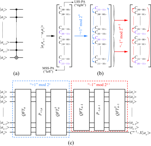
Figure 1: (a) Schematic view of $n$-qubit multi-controlled $X$ gate, (b) illustration of increment/decrements action on the state vector, and (c) implementations block diagram using QFTs and phase gates, adapted from Fig.1 of Ref. [22] originally published in Quantum Information Processing by Springer Nature. In panel (b), MSS-PA (most significant state’s probability amplitude) in classical computing ordering is on the left, while LSS-PA (least significant state’s probability amplitude) is on the right.

2 Related work

Our approach is based on the QFT and inspired by basic quantum arithmetic [21]. One may show that simple QFT-based increment/decrement by one can be used to implement multi-controlled X gates. The equivalence between the QFT-based MCX and the standard one is rigorously proved theoretically [22]. However, a fairly simple explanation can give us an insight into the principles of the proposed implementation. Multi-controlled gate, shown in Fig. 1(a), executes $X$ operation on the highest $n^{\rm th}$ qubit based on the state of $(n-1)$ lower qubits. A pure $n$-qubit state $|a\rangle=|a_{n}a_{n-1}\cdots a_{2}a_{1}\rangle$ is represented by a $2^{n}$ dimensional state vector in Hilbert space. The set of orthonormal basis states $\{|000\cdots 000\rangle,|000\cdots 001\rangle,\cdots,|111\cdots 110\rangle,|111\cdots 111\rangle\}=\{|0\rangle,|1\rangle,\cdots,|2^{n}-2\rangle,|2^{n}-1\rangle\}$ span this linear vector space. Each term in the state vector $C_{|k\rangle}$ (where $k\in\{0,2^{n}-1\}$) is the probability amplitude (weight) of the corresponding basis state. An application of MCX on a $n$-qubit system results in the swap between $C_{|011\cdots 111\rangle}$ and $C_{|111\cdots 111\rangle}$ weights.

Arithmetic operations performed on a $n$-qubit state are congruent modulo $2^{n}$. To implement MCX, we initially increment a qubit state by one. The weight of $|k\rangle$ state becomes the weight of $|(k+1)\mod 2^{n}\rangle$. Thus, all weights are circularly shifted by one, as shown in Fig. 1(b). Performed on a classical register that stores bits, this operation is known as the circular shift to the left. To restore values of control qubits, we have to execute decrements by one on the quantum register comprised of lower $(n-1)$ qubits. Thus, we perform the quantum circular shift to the right in the basis subsets $|0b_{n-1}\cdots b_{m}\cdots b_{1}\rangle$ and $|1b_{n-1}\cdots b_{m}\cdots b_{1}\rangle$ where $b_{m}\in\{0,1\}$, as displayed in Fig. 1(b). As a result, we swapped target states’ probability amplitudes thereby implementing the MCX operation. A block schematic of $n$-qubit MCX implementation is shown in Fig. 1(c).

A standard QFT implementation uses phase gates:

$$R_{m}=P\left(\frac{\pi}{2^{m-1}}\right)=\begin{bmatrix}1&0\\ 0&e^{i\frac{2\pi}{2^{m}}}\end{bmatrix}=\begin{bmatrix}1^{1/2^{m-1}}&0\\ 0&(e^{i\pi})^{1/2^{m-1}}\end{bmatrix}=Z^{1/2^{m-1}}.$$ (1)

Increments and decrements by one can be executed using a QFT-based adder [21]. This method computes QFT on the first addend and uses $R_{m}$ gates to evolve it into QFT of the sum based on the second addend. Then, the inverse of the QFT (QFT^†) returns the result to the computational basis. Thus, the increment by one is executed by $QFT^{\dagger}_{n}P_{+1,n}QFT_{n}|a\rangle=|a+1\mod 2^{n}\rangle=C^{n-1}X|a_{n}\rangle\otimes|a_{n_{c}}+1\mod 2^{n-1}\rangle$, where $P_{+1,n}=Z^{1/2^{n-1}}\otimes Z^{1/2^{n-2}}\otimes\cdots\otimes Z^{1/2}\otimes Z$ and $|a_{n_{c}}\rangle=|a_{n-1}a_{n-2}\cdots a_{2}a_{1}\rangle$ is the register comprised of lower $(n-1)$ control qubits. This part of the schematic is framed by a blue dashed line and labeled by “$+1$”$\mod 2^{n}$ in Fig. 1(c). To restore control qubits to the initial value, we execute decrement by one $I_{2\times 2}\otimes QFT^{\dagger}_{n-1}P_{-1,n-1}QFT_{n-1}(C^{n-1}X|a_{n}\rangle\otimes|a_{n_{c}}+1\mod 2^{n-1}\rangle)=C^{n-1}X|a_{n}\rangle\otimes|a_{n_{c}}\rangle$, where $P_{-1,n-1}={Z^{1/2^{n-2}}}^{\dagger}\otimes\cdots\otimes{Z^{1/2}}^{\dagger}\otimes Z^{\dagger}$ and $I_{2\times 2}$ is the identity $2\times 2$ matrix. This part of the circuit is framed by a red dashed line and labeled by “$-1$”$\mod 2^{n-1}$ in Fig. 1(c).

The decomposition of the circuit from Fig. 1(c) for 5 qubits is shown in Fig. 2. To estimate the time complexity of the circuit, gates that can execute simultaneously are assembled in a single time slot bounded by a vertical dashed gray line in Fig. 2. Control qubits are $|a_{1}\rangle-|a_{4}\rangle$, and the target is $|a_{5}\rangle$. Let us consider the “$+1$”$\mod 2^{5}$ part of the circuit and find the value at the target qubit in the more general case of the $n$-qubit MCX. Controlled phase gates ($C-R_{m}=C-Z^{1/2^{m-1}}$), which act on the target qubit, are represented by gray circles. There are $(2n-1)$ of these gates. The first $(n-1)$ gates (to the left) are conditioned on the qubits of the control register $|a_{c}\rangle=|a_{n-1}\cdots a_{1}\rangle$, the central gate is unconditional, and the last $(n-1)$ gates are controlled by $|a_{c}+1\mod 2^{n-1}\rangle=|a_{n-1}^{\prime}\cdots a_{1}^{\prime}\rangle$. In a simplified notation, the action of these gates on a target wireline is

$$\left({Z^{\frac{a_{n-1}^{\prime}}{2^{1}}}}^{\dagger}{Z^{\frac{a_{n-2}^{\prime}}{2^{2}}}}^{\dagger}\cdots{Z^{\frac{a_{1}^{\prime}}{2^{n-1}}}}^{\dagger}\right){Z^{\frac{1}{2^{n-1}}}}\left(Z^{\frac{a_{1}}{2^{n-1}}}Z^{\frac{a_{2}}{2^{n-2}}}\cdots Z^{\frac{a_{n-1}}{2}}\right)$$

$$=\left(Z^{\frac{2^{0}a_{1}^{\prime}+2^{1}a_{2}^{\prime}+\cdots 2^{n-3}a_{n-2}^{\prime}+2^{n-2}a_{n-1}^{\prime}}{2^{n-1}}}\right)^{\dagger}Z^{\frac{1+2^{0}a_{1}+2^{1}a_{2}+\cdots 2^{n-3}a_{n-2}+2^{n-2}a_{n-1}}{2^{n-1}}}$$

$$={Z^{\frac{1+a_{c}\mod 2^{n-1}}{2^{n-1}}}}^{\dagger}Z^{\frac{1+a_{c}}{2^{n-1}}}.$$ (2)

This expression is the identity in all cases except for $a_{1}=a_{2}=\cdots=a_{n-2}=a_{n-1}=1$ when $(1+a_{c}\mod 2^{n-1})=0$ and $1+a_{c}=2^{n-1}$ so the expression is $Z$. Since $HZH=X$, when the controls are uncomputed by “$-1$”$\mod 2^{n-1}$, the overall circuit executes MCX.

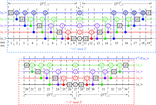
Figure 2: The decomposition of MCX using non-elementary $H$, $R_{m}$ and $C-R_{m}$ gates. The circle indicates phase gate $R_{m}$ with index $m$ inscribed. Gates are divided into time slots by vertical gray dashed lines, where the index of the time slot is denoted at the bottom.

3 Circuit optimization

On the first wireline there is $HR_{1}H=HZH=X$ (slots 9 to 11 in Fig. 2) and $HR_{1}^{\dagger}H=HZ^{\dagger}H=X^{\dagger}=X$ (slots 26 to 28 in Fig. 2). Let’s analyze some circuit simplifications beyond current software optimization capabilities. The phase gates controlled by the first qubit are applied at the beginning of QFT and end of QFT^†. These gates can merge using the equivalence shown in Figs. 3(a) and (b), respectively. We conclude that there is no need to implement $P$ separately. Moreover, the QFT in “$+1$”$\mod 2^{n}$ and the QFT^† in “$-1$”$\mod 2^{n-1}$ will also have a set of $C-R_{m}$ (or $C-R_{m}^{\dagger}$) gates less. Optimized parts of “$+1$”$\>{\rm mod}\>2^{n}$ and “$-1$”$\>{\rm mod}\>2^{n-1}$ circuits are shown in Figs. 3(c) and (d), respectively. A detailed explanation of implementation, calculation of circuit complexities, and proof of principle are elaborated in Ref. [22]. It is straightforward to show that this optimization reduces the number of time slots in MCX by 8. While this optimization merges slots comprising only a few gates, it can still be significant when applying MCX on a small set of qubits. Non-optimized QFT-based MCX becomes less complex than the standard implementation when the number of qubits $n>6$. Using the above optimization, one may show that QFT-MCX is better or just as good as the optimized standard implementation even for $n\leq 6$.

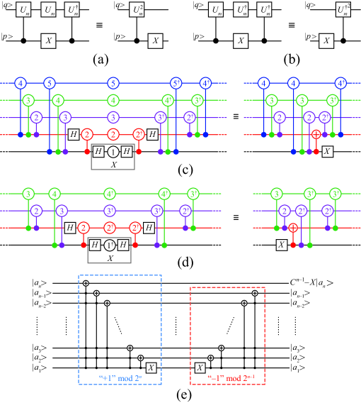
Figure 3: The identities for merging gates in (a) “$+1$”$\>{\rm mod}\>2^{n}$ and (b) “$-1$”$\>{\rm mod}\>2^{n-1}$, where $U_{m}$ is a single qubit unitary gate. (Note: for $U=R_{m}=Z^{1/2^{m-1}}$, $U^{2}=R_{m-1}=Z^{1/2^{m-2}}$). Merging of phase gates and controlled phase gates for 5-qubit MCX in (c) “$+1$”$\>{\rm mod}\>2^{5}$ and (d) “$-1$”$\>{\rm mod}\>2^{4}$ circuits, respectively. (e) An equivalent schematic of QFT-MCX from Fig. 1(c) based on Eq. 3.

Next, we will explain the functionality of “$+1$”$\>{\rm mod}\>2^{n}$ and “$-1$”$\>{\rm mod}\>2^{n-1}$ blocks. Using an iterative approach, we show that the “$+1$”$\mod 2^{n}$ circuit

$$QFT^{\dagger}_{n}P_{+1,n}QFT_{n}|a\rangle=|a+1\mod 2^{n}\rangle$$ (3)

$$= (C_{1}C_{2}\cdots C_{n-2}C_{n-1}-X|a_{n}\rangle)\otimes|a_{n_{c}}+1\mod 2^{n-1}\rangle$$

$$= (C_{1}\cdots C_{n-1}-X|a_{n}\rangle)\otimes(C_{1}\cdots C_{n-2}-X|a_{n-1}\rangle)\otimes|a_{n_{c}-1}+1\mod 2^{n-2}\rangle$$

$$= (C_{1}\cdots C_{n-1}-X|a_{n}\rangle)\otimes\cdots\otimes(C_{1}-X|a_{2}\rangle)\otimes(X|a_{1}\rangle),$$

is equivalent to the stair-wise array of controlled $X$ gates, and “$-1$”$\mod 2^{n}$ is its inverse. From this perspective, the schematic view of the MCX circuit is given in Fig. 3(e).

We noticed that Qiskit’s transpile function automatically handles the following optimization. Different forms of $C-R_{m}$ decompositions are schematically displayed in Fig. 4(a). The control phase gate $C_{p}-R_{m,q}$ applied to $|a_{p}\rangle$ as the control and $|a_{q}\rangle$ ($q>p$ in Fig. 2) as the target is

$$(I_{2\times 2}\otimes P(\frac{\pi}{2^{m}}))(C-X)(I_{2\times 2}\otimes P(-\frac{\pi}{2^{m}}))(C-X)(P(\frac{\pi}{2^{m}})\otimes I_{2\times 2})(|a_{p}\rangle\otimes|a_{q}\rangle)$$ (4)

$$= (I_{2\times 2}\otimes R_{z}(\frac{\pi}{2^{m}}))(C-X)(I_{2\times 2}\otimes R_{z}(-\frac{\pi}{2^{m}}))(C-X)(P(\frac{\pi}{2^{m}})\otimes I_{2\times 2})(|a_{p}\rangle\otimes|a_{q}\rangle)$$

$$= (C-R_{z}(\frac{\pi}{2^{m-1}}))({\color[rgb]{1,0,1}P(\frac{\pi}{2^{m}})}\otimes I_{2\times 2})(|a_{p}\rangle\otimes|a_{q}\rangle),$$

where we used the identity $P(\gamma)XP(-\gamma)=R_{z}(\gamma)XR_{z}(-\gamma)$.

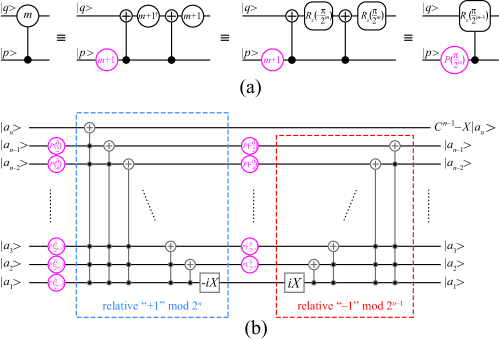
Figure 4: (a) Decompositions of $C-R_{m}$ gates using $R_{m+1}=P(\frac{\pi}{2^{m}})$ (marked by circles) and $R_{z}(\pm\frac{\pi}{2^{m}})$ gates (marked with rounded squares). (b) A schematic of the simplified QFT-MCX obtained by omitting the phase correction gates $P$ from $C-R_{m}$ acting on control wirelines. A gray color of multi-controlled gates indicates a relative phase $-i$ and $+i$ on gates in the “$+1$” and “$-1$” blocks, respectively.

A phase difference between $C-R_{m}$ and $C-R_{z}(\frac{\pi}{2^{m-1}})$ gates is compensated using the ${\color[rgb]{1,0,1}R_{m+1}=P(\frac{\pi}{2^{m}})}$ gate on the control wireline of the $C-R_{z}$ gate, as explained in Ref. [6]. If we neglect the phase-adding ${\color[rgb]{1,0,1}P}$ gates and use $C-R_{z}$ instead of $C-R_{m}$, providing that all qubits lower than the selected one are in the state $|1\rangle$, $R_{z}(\pi)=-iZ$ will be implemented between the two Hadamard gates in “$+1$”$\>{\rm mod}\>2^{n}$ instead of $Z$ (see Fig. 2 and Eq. 2). These omitted $P$ gates implement the phase factor $i$, which can be easily verified in Fig. 2. Due to this phase relativization, we will implement multi-controlled $(-iX)$ gates in “$+1$”$\>{\rm mod}\>2^{n}$. Similarly, multi-controlled $(iX)$ gates are implemented in “$-1$”$\>{\rm mod}\>2^{n-1}$ subcircuit. Since $-i\cdot i=1$, it will not affect the control qubits outputs. Moreover, based on the symmetry argument and using the decomposition of $C-R_{m}$ from Fig. 4(a), it is straightforward to show that on each control wireline, displayed in Fig. 2, these $P$ gates cancel out if all lower control qubits are one (when we have $P(\frac{\pi}{2^{m}})XP(-\frac{\pi}{2^{m}})P(\frac{\pi}{2^{m}})XP(-\frac{\pi}{2^{m}})=I_{2\times 2}$), or if they are not (when we have $P(\frac{\pi}{2^{m}})P(-\frac{\pi}{2^{m}})P(\frac{\pi}{2^{m}})P(-\frac{\pi}{2^{m}})=I_{2\times 2}$). However, this doesn’t apply to the $C-R_{m}$ gates acting on the target wireline (see gray gates in Fig. 2), where the “inverted” sequence of gates in “$-1$” block-circuit (which would perform “uncomputation”) is omitted. Therefore, the $P$ gates appearing in the $C-R_{z}$ decomposition of the $C-R_{m}$ gates acting on the target wireline can not be omitted. In Fig. 4(b) we show an equivalent schematic of QFT-MCX based on the relative phase multi-controlled $(\mp iX)$ gates comprised of $C-R_{z}$s and additional $P$ gates originated from $C-R_{m}$ acting on the target qubit. We used the notation $P(\delta/2^{m-1})$ instead of $R_{m}=P(\pi/2^{m-1})$, to consider a general case of controlling the phase-factor application ($e^{i\delta}$) to the target qubit.

If all controls are $|1\rangle$, $-iX$ is implemented to the target qubit. To correct the additional phase ($-i$), we need to implement the phase factor $e^{i\delta}=e^{i\pi/2}=i$ to the target qubit by adding $P(\delta/2)$ and $P(-\delta/2)$ to the $(n-1)$th wireline, as shown in Fig. 4(b), thereby implementing

$$XP\left(-\frac{\delta}{2}\right)XP\left(\frac{\delta}{2}\right)=R_{z}(\delta)=e^{-i\delta/2}P(\delta).$$ (5)

By doing this, we introduce the phase factor $e^{-i\delta/2}$ to the $(n-1)$th wireline, which can be corrected by adding $P(\delta/4)$ and $P(-\delta/4)$ to the $(n-2)$th wireline, as shown in Fig. 4(b). However, this results in the additional phase $e^{-i\delta/4}$ (the wireline output is $e^{-i\delta/4}P(\delta/2)$, based on Eq. 5), which can be corrected by adding appropriate phase gates to the lower qubit, and so on. Phase gates used to add $e^{i\delta}$ are displayed in magenta in Fig. 4(b). One may note that these gates annihilate if one of the control qubits is in $|0\rangle$ state. Moreover, the same phase-adding circuit can be implemented by surrounding the “$-1$”$\>{\rm mod}\>2^{n-1}$ subcircuit with the same phase gates, but in reverse ordering to the one used in the “$+1$”$\>{\rm mod}\>2^{n}$. Thereby, on the $(n-1)$th wireline we implement

$$P\left(\frac{\delta}{2}\right)XP\left(-\frac{\delta}{2}\right)X=R_{z}(\delta)=e^{-i\delta/2}P(\delta),$$ (6)

providing that all controls are $|1\rangle$. Alternatively, we may combine the two methods.

Figure 5: A schematic of five-qubit MCU implementations based on QFT-MCX modification in the (a) fully connected (FC) and (b) linear nearest-neighbor (LNN) quantum computer architecture. Circles denote either phase $R_{m}=Z^{1/2^{m-1}}$ or $R_{z}(\pi/2^{m-1})$ gates, while hexagons represent special unitary $U_{m}=U^{1/2^{m-1}}$ gates ($U_{m}(2)=e^{i\delta}U_{m}$), with the value $m$ inscribed into gate symbols. To estimate the time complexity, gates that can execute simultaneously are divided into time slots. We do not assign a number for the time slot comprising $P$ gates, since these gates are an integral part of $C-U_{m}(2)$.

4 Multi-controlled U(2) gates

The aim is to generalize the MCX circuit to a multi-controlled single-qubit unitary gate (MCU). We will explore implementations in two distinct quantum computer architectures to find the lower and upper bounds for the time and space complexities. The most favorable architecture supports interaction between arbitrary pairs of qubits, implying that the system is fully connected (FC). Implementation in this architecture is the least complex, setting the lower complexity bounds. The most restricted is the linear one allowing interactions only between nearest-neighbours (LNN). Using this architecture demands swapping many qubits to perform two-qubit gates, and additional SWAP gates increase the time and space complexities. We use two strategies to generalize the circuit. The first is based on modifying the QFT-based MCX gate, while the second uses extended optimized MCX gates and well-known ZYZ ($ABC$) decomposition [6].

It is straightforward to conclude from Eq. 2 that by substituting $R_{m}=Z^{1/2^{m-1}}$ with $U_{m}=U^{1/2^{m-1}}$ on the target qubit and omitting $H$ gates, the circuit implements a multi-controlled unitary $U$ gate. Schematic views of 5-qubit MCUs in the FC and LNN architecture are given in Figs. 4(a) and (b), respectively. If $U$ is not a special unitary, then $U(2)=e^{i\delta}SU(2)$, where $\delta$ is a real valued. To implement an arbitrary multi-controlled $U(2)\not\in SU(2)$, we need to implement multi-controlled $SU(2)$ and the controlled phase circuit $C_{1}C_{2}\cdots C_{n-2}-P_{n-1}(\delta)$ that adds the phase factor $e^{i\delta}$, as shown in the inset in Fig. 4(a). In section 3 we found that the “$+1$” and “$-1$” blocks comprised a sequence of multi-controlled gates needed to implement $(n-1)$-controlled phase gate. So, you don’t need to implement it using a separate circuit. Moreover, these gates can be found by direct decomposition of controlled-$U(2)$ gate

$$C-U(2)^{1/2^{m-1}}=C-U^{1/2^{m-1}}(P(\delta/2^{m-1})\otimes I_{2\times 2}).$$ (7)

Therefore, we have not assigned them a separate time slot in Fig. 5. Furthermore, the phase gate executes simultaneously with a gate acting on the controlled wireline.

One may show that FC QFT-MCU executes in $(8n-18)$ time slots. It comprises of $4(n-3)$ single-qubit Hadamards, $2(n-1)(n-3)$ controlled phase gates, two $C-$NOTs and $(2n-3)$ $C-U^{1/2^{m-1}}$ gates. An approximate QFT (AQFT) may provide greater accuracy than a full QFT in the presence of decoherence [23]. Controlled phases $R_{m}$ with $m\leq[\log_{2}n]$ are used in AQFT. Therefore, the number of controlled gates reduces to $2([\log_{2}n]-1)(2n-3-[\log_{2}n])$ and $2([\log_{2}n]-1)$, $C-R_{m}$ and $C-U_{m}$ gates, respectively.

Using the systematic approach for swapping qubits in finite-neighbor quantum architectures [24], one may find that LNN QFT-MCU needs $(8n-20)$ time slots with $(2n^{2}-6n+6)$ SWAP gates. Therefore, LNN uses approximately twice the number of time slots and gates as FC QFT-MCU, thus setting the upper bound for the time and space complexities. In the LNN architecture, SWAP and $C-R_{m}$ are neighboring. Reducing $C-R_{m}$ to $C-R_{z}$ gate, some of $C-X$ gates cancel out between SWAP and $C-R_{z}$. Hence, when utilizing certain software optimizations, the upper limit is lower than the one derived above.

Actual circuit depth and the number of gates implemented depend on the native gate set (NGS) of the quantum device used in the calculation. The decomposition of a non-elementary gate uses a few elementary gates executed in a certain number of time slices. This number of time slices defines the circuit depth. One should note that some elementary gates can be executed in parallel and some cancel out, as explained in Ref. [22] for the selected NGS. Elementary gates that comprise the NGS have a high but finite fidelity. Also, current quantum devices are prone to noise and decoherence. Therefore, low-depth circuits using fewer elementary gates are less prone to errors.

The advantage of using QFT to implement MCU relies on the efficient decomposition of controlled phase gates. The state-of-the-art linear-depth decomposition (LDD) of MCU [16, 18] use $C-X^{1/2^{m-1}}$ and $C-U_{m}=C-U^{1/2^{m-1}}$ gates. A recent paper showed that the circuit can be simplified by omitting gates with $m>\lceil\log_{2}n\rceil$ [18] similar to the approximate QFT approach. We should note that the QFT-based MCU circuit uses approximately the same number of non-elementary gates as the state-of-the-art one. However, the decomposition of $C-R_{m}$ in the NGS of superconducting hardware is twice as less complex as $C-X^{1/2^{m-1}}$ leading to approximately double the advantage of the QFT-based approach when implementing MCX [22]. In the case of a random special unitary gate, the depth of the MCU circuit is predominantly determined by the complexity of the $C-U_{m}$ decomposition. Since our approach uses the same sequence of gates on the target qubit wireline, the difference in the depths will be smaller than in the case of MCX. However, the number of elementary gates in our approach is still twice as small.

The main problem in using the $C-R_{x}$ [16, 18] and QFT-based MCU decomposition is related to the complexity and precision of $C-U_{m}$ implementation. Moreover, a similar issue exists for $C-X^{1/2^{m-1}}$ and $C-R_{m}$, but it is less pronounced in the QFT-based approach since the latter has a simple decomposition.

A more effective circuit can be obtained using the ZYZ decomposition. For a single-qubit unitary matrix expressed as $U=e^{i\delta}R_{z}(\alpha)R_{y}(\theta)R_{z}(\beta)$, there is a set of matrices $A=R_{z}(\alpha)R_{y}(\theta/2)$, $B=R_{y}(-\theta/2)R_{z}(-(\alpha+\beta)/2)$, and $C=R_{z}((\beta-\alpha)/2)$ such that $ABC=I_{2\times 2}$ and $U=e^{i\delta}AXBXC$ [6]. To implement two MCX gates needed for $ABC$-based MCU, we will use a single QFT-based MCX circuit with “$-1$”$\mod 2^{n}$ instead of $I_{2\times 2}\otimes$(“$-1$”$\mod 2^{n-1}$), as shown in Fig. 6. Therefore, the complexity of the circuit is approximately equal to the QFT-MCX, where we use only additional $A$, $B$, and $C$ single-qubit gates found by ZYZ decomposition of $U\in SU(2)$. Detailed schematics of QFT-MCX in FC and LNN architectures can be found in Ref. [22]. In general multi-controlled single-qubit $U(2)$ gate implementation, we have additional phase gates (shown in magenta color in Fig. 6), that implement $(n-1)$-qubit controlled phase gate. This doesn’t affect the MCU’s time complexity, since $P$ gates can be executed parallel with $A$ and $B$.

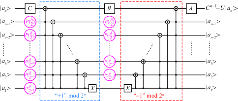
Figure 6: A schematic of $n$-qubit MCU implementation based on the ZYZ decomposition and QFT.

The QFT-based subcircuits (“$+1$” and “$-1$”) implement two MCX gates and are executed in $(8n-12)$ time slots in the FC architecture. There are $4(n-2)$ Hadamard gates, $2n(n-2)$ controlled phases, and two $C-X$ gates. AQFT reduces the number of $C-R_{m}$ gates to $2([\log_{2}n]-1)(2n-1-[\log_{2}n])$. At most three time slots are required for executing $A$, $B$, and $C$. These gates use a total of three $R_{z}$ and two $R_{y}$ gates. The LNN implementation uses an additional $(8n-16)$ time slots with $2(n-1)^{2}$ SWAP gates. Again, canceling out some $C-X$ gates between SWAP and $C-R_{z}$ the upper bound will be lower than it seems.

5 Analytical and numerical analysis

To get theoretical bounds for complexities in a genuine quantum computation, we addopt the native gate set $\{C-X,R_{z},ID,SX=\sqrt{X},X\}$, which is one of a few sets used by superconducting hardware. One may show that $R_{m}=\exp(i\frac{\pi}{2^{m}})\cdot R_{z}(\frac{\pi}{2^{m-1}})$, $H=\exp(i\frac{\pi}{4})\cdot R_{z}(\frac{\pi}{2})\sqrt{X}R_{z}(\frac{\pi}{2})$, $R_{y}=\sqrt{Z}HR_{z}H\sqrt{Z}^{\dagger}$, and $SWAP_{12}=(C_{1}-X_{2})(C_{2}-X_{1})(C_{1}-X_{2})$[7]. Hadamard and SWAP use three native gates and three elementary time intervals to execute, while $R_{y}$ and $C-R_{m}$ use five. Employing parallelization, the depths of $H$ and $C-R_{m}$ gates are effectively reduced to two and four, respectively. Some of the $R_{z}$ gates can be executed simultaneously, and some will merge or cancel out, as elaborated in Ref. [22]. Merging consecutive $R_{z}$ gates, $A$ and $B$ comprise 5 elementary gates, and $C$ uses one $R_{z}$ gate. There are two $SWAP\cdot C-X$ gates in the LNN implementation, where two $C-X$ gates annihilate in each. In the most general case, the decomposition of a controlled single-qubit unitary gate in the NGS uses 14 elementary gates (two $C-X$, four $\sqrt{X}$, and the rest are $R_{z}$) that execute in 13 elementary time intervals. Merging $R_{z}$’s of neighboring $U_{m}$ gates, the depth and the number of elementary gates effectively reduce by one (except for the first or the last gate on the target wireline). One should note that the decomposition of some $C-U$ gates (excluding $C-X$ or $C-Z$, since comprised in the basis gate set of superconducting quantum devices) is less complex, where $C-R_{z}$ and $C-P$ are some of the simplest. In the approximate form of QFT-MCU, we will use $R_{m}$ (or $R_{z}(\pi/2^{m-1})$) and $U_{m}$ with $m\leq\lceil\log_{2}n\rceil$, which results in a low error [18]. We will derive the lower and upper bounds for the circuit depth and number of elementary gates for a multi-controlled $U(2)$ gate. All bounds, expressed as a function of the number of qubits used, are derived using the selected NGS. We will not use any additional specific optimization available in quantum computing software.

By counting in the NGS, FC-MCU based on MCX modification has the depth $(34n-56)$. The circuit uses $(6n^{2}-8n-13)$ $R_{z}$, $12(n-2)$ $\sqrt{X}$ or $\sqrt{X}^{\dagger}$, and $4(n^{2}-3n+4)$ $C-X$ gates. If we omit redundant $P$ gates (in simplifying $C-R_{m}$ to $C-R_{z}$), the number of $R_{z}$ gates can be reduced by $2(n-1)(n-3)$. By approximating the QFT, the number of $R_{z}$, $\sqrt{X}$, and $C-X$ gates wil be reduced by $6(n^{2}-4n-(\lceil\log_{2}n\rceil-1)(2n-5-\lceil\log_{2}n\rceil))$, $4(2n-2-2(\lceil\log_{2}n\rceil-1))$, and $2(2n(n-3)-2(\lceil\log_{2}n\rceil-1)(2n-2-\lceil\log_{2}n\rceil))$, respectively. Due to additional SWAP gates used, the depth of the LNN circuit is greater by $(24n-64)$ for $n>3$. Also, the number of $C-X$ gates increases by $(6n^{2}-18n+14)$. Annihilating some $C-X$ gates between neighboring $C-R_{z}$ and SWAP gates, one may reduce the $C-X$ count by $4(n-1)(n-3)$. For general $U(2)$, we use $(2n-3)$ $R_{z}$ gates to implement the controlled-phase circuit.

FC-MCU based on the ZYZ decomposition has the depth $(32n-44)$. It uses $(6n^{2}-8n-4)$ $R_{z}$, $4(n-1)$ $\sqrt{X}$ or $\sqrt{X}^{\dagger}$, and $(4n^{2}-6)$ $C-X$ gates. Using AQFT will reduce the number of $R_{z}$ and $C-X$ gates by $6(n(n-2)-(\lceil\log_{2}n\rceil-1)(2n-1-\lceil\log_{2}n\rceil))$ and $4(n(n-2)-(\lceil\log_{2}n\rceil-1)(2n-1-\lceil\log_{2}n\rceil))$, respectively. Due to additional SWAP gates used, the depth of the LNN circuit is greater by $(24n-52)$ for $n>3$, while the number of $C-X$ gates increases by $(6n^{2}-12n+2)$. Using additional optimization, the number of $R_{z}$ and $C-X$ gates can be reduced by $2n(n-2)$ and $4n(n-2)$, respectively. This circuit also uses $(2n-3)$ $R_{z}$ gates to implement $e^{i\delta}$.

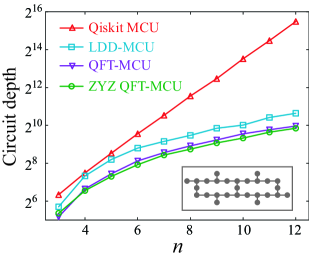
Figure 7: The dependence of circuit depths on the number of qubits in default Qiskit ($\bigtriangleup$), LDD-MCU from Ref. [16] ($\Box$), QFT-MCU ($\bigtriangledown$), and ZYZ QFT-MCU ($\bigcirc$). The layout of the quantum processor is shown in the inset.

We consider the AQFT FC-MCU the lower and LNN-MCU the upper bound on the number of elementary gates and the circuit depth in a genuine quantum computation. Actual complexities for application on a quantum device are obtained by assembling analyzed circuits using the transpile function built-in Python package Qiskit v.0.42.1 [25]. In doing so, we used optimization level 3. To remove any doubt about bias in our implementation, we used the local simulator to transpile circuits for application on the ‘ibm_hanoi’ employed in Refs. [16, 18] although it was retired recently. We compare our implementations to the standard Qiskit and the state-of-the-art MCU circuit. The unitary single-qubit gate used in all analyzed MCU circuits was randomly chosen from $SU(2)$ gates. To get angles $\alpha$, $\theta$, and $\beta$, we have generated random rational numbers and multiplied them by $\pi$. We constrained our choice to exclude trivial gates. The comparison of circuit depths is displayed in Fig. 7.

The default Qiskit implementation performs the worst exhibiting an exponential increase in time complexity with the number of qubits. Circuit depths of either LDD or QFT-based MCUs are linear in the number of qubits. Both LDD and QFT-MCU use $C-U_{m}$ gates which have a complex decomposition. It increases the circuit depth compared to MCX implementation. However, LDD uses $C-R_{x}$ gates that are more complex than $C-R_{m}$ comprising QFT-based implementation. Therefore, the circuit depths of LDD-MCU are larger than QFT-MCU although they have a similar construction. Finally, the ZYZ-based decomposition of the QFT-MCU is approximately as complex as the MCX circuit, thus exhibiting the least circuit depth of all implementations. Not only does it use the smallest number of elementary gates and have the lowest circuit depth, but it also doesn’t employ $C-U_{m}$ gates. To implement $U^{1/2^{m-1}}$ we have to use gates having small angles as the argument if $m$ is large. A matrix representation of small-angle gates is close to the unity matrix. Therefore, it is debatable if the LDD and the QFT-MCU that use $U_{m}$ can be implemented with sufficient precision in a genuine quantum device.

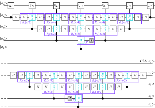
Figure 8: Simplification of LDD-MCU to our QFT-MCU. Pairs of Hadamard gates (${\color[rgb]{.5,.5,.5}HH}=I_{2\times 2}$) added to the LDD-MCU are shown by gray-outlined squares ($\Box$), where the two constant phase gates $\pm iI_{2\times 2}$ are given by small gray squares ($\blacksquare$).

Following the discussion in section 3, one may wonder if LDD-MCU can be simplified. We found that if we insert two consecutive Hadamard gates between $R_{x}$ gates from Ref. [16, 18] (where $HH=I_{2\times 2}$), and using the equivalence $HR_{x}(\gamma)H=R_{z}(\gamma)$, all the $C-R_{x}(\gamma)$ gates will transform to $C-R_{z}(\gamma)$. On the second wireline $R_{x}(\pm\pi)=\mp iX$. We can add two constant phase gates, $+iI_{2\times 2}$ and $-iI_{2\times 2}$, between $R_{x}$ gates transforming $C-R_{x}(\pm\pi)$ to $C-X$ gates. When we perform all transformations above, each control wireline, except the first two, will have one $H$ gate ‘remaining’ at the beginning and the end of the $C-R_{z}$ sequence. Thus, the LDD-MCU is reduced to our QFT-MCU from Fig. 5, as demonstrated in Fig. 8, which will decrease the number of gates used and the LDD circuit depth by approximately twice.

6 Conclusions

In this paper, we have presented two new implementations of multi-controlled unitary (MCU) gates. The first implementation is based on the modification of a multi-controlled X (MCX) gate that uses the quantum Fourier transform (QFT), where the phase gates acting on the target qubit ($Z^{1/2^{m-1}}$) are replaced with the adequate roots of the single-qubit unitary gate ($U^{1/2^{m-1}}$). This is similar to the state-of-the-art LDD circuit but has a lower circuit depth and uses approximately twice as few elementary gates. The main disadvantage of the former two implementations is that they both use $U^{1/2^{m-1}}$ gates, which are hard to implement with desired precision. The second implementation is based on the ZYZ decomposition and uses an extended QFT-based MCX circuit to implement the two MCX gates needed for the decomposition. This implementation has lower time and space complexities compared to any existing MCU. Simplification of this circuit can be achieved straightforwardly using an approximation of the QFT or by introducing auxiliary qubits, which was elaborated in our previous work on the MCX. The supremacy of our implementations was demonstrated by analyzing transpiled circuits, where our MCUs exhibited a noticeable advantage compared to the existing state-of-the-art implementation.

We elaborated various techniques to optimize our circuits. Moreover, we demonstrated that the state-of-the-art LDD-MCU can be simplified to our QFT-MCU based on QFT-MCX modification, thus significantly reducing the LDD’s time and space complexities.

Acknowledgements

This work was financially supported by the Ministry of Science, Technological Development and Innovation of the Republic of Serbia under contract number: 451-03-65/2024-03/200103.

References

- \bibcommenthead
- Preskill [2018] Preskill, J.: Quantum Computing in the NISQ era and beyond. Quantum 2, 79(2018). https://doi.org/10.22331/q-2018-08-06-79
- Kim et al. [2023] Kim, Y., Eddins, A., Anand, S., Wei, K.X., van den Berg, E., Rosenblatt, S., Nayfeh, H., Wu, Y., Zaletel, M., Temme, K., Kandala, A.: Evidence for the utility of quantum computing before fault tolerance. Nature 618, 500–505 (2023). https://doi.org/10.1038/s41586-023-06096-3
- Plesch [2011] Plesch, M., Brukner, Č.: Quantum-state preparation with universal gate decompositions. Phys. Rev. A 83(3), 032302 (2011). https://doi.org/10.1103/PhysRevA.83.032302
- Zhang [2021] Zhang, X.-M., Yung, M.-H., Yuan, X.: Low-depth quantum state preparation. Phys. Rev. Res. 3(4), 043200 (2021). https://doi.org/10.1103/PhysRevResearch.3.043200
- Araujo [2021] Araujo, I.F., Park, D.K., Petruccione, F., da Silva, A.J.: A divide-and-conquer algorithm for quantum state preparation. Sci. Rep. 11(1), 6329 (2021). https://doi.org/10.1038/s41598-021-85474-1
- Barenco et. al [1995] Barenco, A., Bennett, C.H., Cleve, R., DiVincenzo, D.P., Shor, P., Sleator, T., Smolin, J.A., Weinfurter, H.: Elementary gates for quantum computation. Phys. Rev. A 52(5), 3457–3467 (1995). https://doi.org/10.1103/PhysRevA.52.3457
- Nielsen and Chuang [2010] Nielsen, M.C., Chuang, I.L.: Quantum Computation and Quantum Information. Cambridge University Press, New York (2010). ISBN 978-1-107-00217-3
- Shende [2006] Shende, V.V., Bullock, S.S., Markov, I.L.: Synthesis of quantum-logic circuits. IEEE Transactions on CAD 25(6), 1000–1010 (2006). https://doi.org/10.1109/TCAD.2005.855930
- Malvetti [2021] Malvetti, E., Iten, R., Colbeck, R.: Quantum circuits for sparse isometries. Quantum 5, 412 (2021). https://doi.org/10.22331/q-2021-03-15-412
- Bae et. al [2020] Bae, J.-H., Alsing, P.M., Ahn, D., Miller, W.A.: Quantum circuit optimization using quantum Karnaugh map. Sci. Rep. 10(1), 15651 (2020). https://doi.org/10.1038/s41598-020-72469-7
- Brugiere et. al [2021] de Brugière, T.G., Baboulin, M., Valiron, B., Martiel, S., Allouche, C.: Reducing the depth of linear reversible quantum circuits. IEEE Trans. Quantum Eng. 2, 3102422 (2021). https://doi.org/10.1109/TQE.2021.3091648
- Cuomo et. al [2023] Cuomo, D., Caleffi, M., Krsulich, K., Tramonto, F., Agliardi, G., Prati, E., Cacciapuoti, A.S.: Optimized compiler for distributed quantum computing. ACM T. Quantum Comput. 4(2), 15 (2023). https://doi.org/10.1145/3579367
- Saeedi and Pedram [2013] Saeedi, M., Pedram, M.: Linear-depth quantum circuits for -qubit Toffoli gates with no ancilla. Phys. Rev. A 87(6), 062318 (2013). https://doi.org/10.1103/PhysRevA.87.062318
- Maslov [2016] Maslov, D.: Advantages of using relative-phase Toffoli gates with an application to multiple control Toffoli optimization. Phys. Rev. A 93(2), 022311 (2016). https://doi.org/10.1103/PhysRevA.93.022311
- Jun and Choi [2023] Jun, J.-M., Choi, I.-C.: Optimal multi-bit Toffoli gate synthesis. IEEE Access 11, 27342–27351 (2023). https://doi.org/10.1109/ACCESS.2023.3243798
- Silva and Park [2022] da Silva, A.J., Park, D.K.: Linear-depth quantum circuits for multiqubit controlled gates. Phys. Rev. A 106(4), 042602 (2022). https://doi.org/10.1103/PhysRevA.106.042602
- Vale et. al [2023] Vale, R., Azevedo, T.M.D., Araújo, I.C.S., Araujo, I.F., da Silva, A.J.: Circuit decomposition of multicontrolled special unitary single-qubit gates. IEEE Transactions on CAD 43(3), 802–811 (2023). https://doi.org/10.1109/TCAD.2023.3327102
- Silva et. al [2023] Silva, J.D.S., Azevedo, T.M.D., Araujo, I.F., da Silva, A.J.: Linear decomposition of approximate multi-controlled single qubit gates (2023). https://doi.org/10.48550/arXiv.2310.14974
- He et. al [2017] He, Y., Luo, M.-X., Zhang, E., Wang, H.-K., Wang, X.-F.: Decompositions of n-qubit Toffoli gates with linear circuit complexity. Int. J. Theor. Phys. 56, 2350–2361 (2017). https://doi.org/10.1007/s10773-017-3389-4
- Balauca and Arusoaie [2022] Balauca, S., Arusoaie , A.: Efficient constructions for simulating multi controlled quantum gates. In: Groen, D., de Mulatier, C., Paszynski, M., Krzhizhanovskaya, V.V., Dongarra, J.J., Sloot, P.M.A. (eds.) Computational Science - ICCS 2022, vol. 13353, pp. 179–194. Springer International Publishing, Cham (2022) ISBN 978-3-031-08759-2 https://doi.org/https://doi.org/10.1007/978-3-031-08760-8_16
- Draper [2000] Draper, T.G.: Addition on a Quantum Computer (2000). https://doi.org/10.48550/arXiv.quant-ph/0008033
- Arsoski [2024] Arsoski, V.V.: Implementing multi-controlled X gates using the quantum Fourier transform. Accepted for publication in Quantum Inf. Process. on 2024-08-06 (2024). https://doi.org/https://doi.org/10.48550/arXiv.2407.18024
- Barenco et. al [1996] Barenco, A., Ekert, A., Suominen, K.-A., Törmä, P.: Approximate quantum Fourier transform and decoherence. Phys. Rev. A 54(1), 139–146 (1996). https://doi.org/10.1103/PhysRevA.54.139
- Maslov [2007] Maslov, D.: Linear depth stabilizer and quantum Fourier transformation circuits with no auxiliary qubits in finite-neighbor quantum architectures. Phys. Rev. A 76(5), 052310 (2007). https://doi.org/10.1103/PhysRevA.76.052310
- QISKit SDK [2017] https://pypi.org/project/qiskit/