Reclaiming Residual Knowledge: A Novel Paradigm to Low-Bit Quantization

Abstract

This paper explores a novel paradigm in low-bit (i.e. 4-bits or lower) quantization, differing from existing state-of-the-art methods, by framing optimal quantization as an architecture search problem within convolutional neural networks (ConvNets). Our framework, dubbed CoRa (Optimal Quantization Residual Convolutional Operator Low-Rank Adaptation), is motivated by two key aspects. Firstly, quantization residual knowledge, i.e. the lost information between floating-point weights and quantized weights, has long been neglected by the research community. Reclaiming the critical residual knowledge, with an infinitesimal extra parameter cost, can reverse performance degradation without training. Secondly, state-of-the-art quantization frameworks search for optimal quantized weights to address the performance degradation. Yet, the vast search spaces in weight optimization pose a challenge for the efficient optimization in large models. For example, state-of-the-art BRECQ necessitates $2\times 10^{4}$ iterations to quantize models. Fundamentally differing from existing methods, CoRa searches for the optimal architectures of low-rank adapters, reclaiming critical quantization residual knowledge, within the search spaces smaller compared to the weight spaces, by many orders of magnitude. The low-rank adapters approximate the quantization residual weights, discarded in previous methods. We evaluate our approach over multiple pre-trained ConvNets on ImageNet. CoRa achieves comparable performance against both state-of-the-art quantization-aware training and post-training quantization baselines, in $4$-bit and $3$-bit quantization, by using less than $250$ iterations on a small calibration set with $1600$ images. Thus, CoRa establishes a new state-of-the-art in terms of the optimization efficiency in low-bit quantization. Implementation can be found on https://github.com/aoibhinncrtai/cora_torch.

Keywords Low-Bit Quantization  $\cdot$ Architecture Search  $\cdot$ Neural Combinatorial Optimization  $\cdot$ Optimization

1 Introduction

ConvNets (Li et al., 2021a; Awais et al., 2023) are favored as vision foundation models, offering distinct advantages such as the inductive bias in modeling visual patterns (Wang and Wu, 2024; d’Ascoli et al., 2019; Hermann et al., 2020), efficient training, and hardware-friendliness (Maurício et al., 2023). Network quantization is indispensable in enabling efficient inference when deploying large models on devices with limited resources (Han et al., 2015; Neill, 2020; Mishra et al., 2020; Liang et al., 2021). Representing floating-point tensors as integers significantly reduces the computational requirements and memory footprint.

Yet, low-bit quantization often leads to severe performance degradation (Choukroun et al., 2019; Gholami et al., 2022; Li et al., 2023). For example, the standard accuracy of a resnet18, pretrained on ImageNet (Deng et al., 2009), plummets to a mere $1.91\%$ from $67.32\%$, with 4-bit weight-only quantization (WOQ), using min-max clipping (Nagel et al., 2021). To tackle this issue, two research lines are undertaken: quantization-aware training (QAT) and post-training quantization (PTQ) (Gholami et al., 2022; Nagel et al., 2020; Guo, 2018).

QAT methods seek the optimal quantized weights during the training process to minimize performance degradation. Despite their promising performance, the substantial computational and data requirements pose major challenges in deployment efficiency. For instance, the state-of-the-art PACT (Choi et al., 2018) entails a minimum of $10^{8.12}$ iterations with $1.2M$ training samples to converge on ImageNet. Additionally, empirical evidence shows that QAT methods often yield very limited performance at low-bit quantization due to optimization difficulty (Nagel et al., 2022; Liu and Mattina, 2019; Esser et al., 2019). PTQ methods, e.g. AdaRound (Nagel et al., 2020) and BRECQ (Li et al., 2021b), overcome these limitations by reconstructing the optimal quantized weights of pre-trained models, with optimization on small calibration sets; these potentially reduce computational and data requirements.

Notably, both state-of-the-art QAT and PTQ methods quantize models by optimizing within weight spaces. Their optimization efficiencies are substantially hindered by the vast dimensions of search spaces. For example, a resnet50 contains over 2.5M trainable parameters (He et al., 2016), suggesting a search space of the dimension of $\mathbb{R}^{25,000,000}$. The state-of-the-art PTQ method BRECQ needs at least $2\times 10^{4}$ iterations to converge for a resnet50 pre-trained on ImageNet.

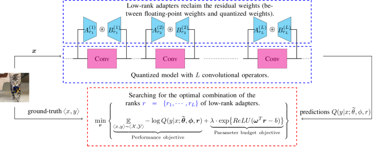
Figure 1: CoRa framework: Searching for the optimal adapters, reclaiming the quantization residual knowledge, instead for the optimal quantized weights. The low-rank convolutional adapter at the $l$-th layer $B_{r_{l}}^{(l)}\circledast A_{r_{l}}^{(l)}$ is determined by a discrete integer $r_{l}$.

This research delves into a question: “Beyond the quantization methods with weight space optimization, does an alternative paradigm exist?”. Intuitively, the quantization residual knowledge – namely, the quantization residual weights between floating-point weights and quantized weights – retains vital information lost during the quantization process. This quantization residual knowledge, which has long been overlooked by the research community, holds the potential value that reverses performance degradation without training. Motivated by this perspective, our approach, CoRa, as shown in Figure 1, explores a novel paradigm, differing from state-of-the-art QAT and PTQ methods: by seeking the optimal low-rank adapters (Hu et al., 2021), reclaiming the residual knowledge; thus reversing the performance degradation, and establishing a new state-of-the-art in terms of the optimization efficiency.

A low-rank adapter consists of two cascaded convolutional filters (e.g. $A$ and $B$) with significantly lower sizes, which are directly converted from high-rank quantization residual weights. As shown in Figure 1, the $l$-th layer adapter $B_{r_{l}}^{(l)}\circledast A_{r_{l}}^{(l)}$, with a low rank $r_{l}$, is attached to the $l$-th layer convolutional filter, and approximates the quantization residual weights. CoRa seeks the optimal ranks $r=\{r_{1},\cdots,r_{L}\}$ for all adapters. Surprisingly, earlier works (Zhang et al., 2015; Yang et al., 2020; Hu et al., 2021; Denton et al., 2014; Rigamonti et al., 2013; Jaderberg et al., 2014; Zhong et al., 2024) do not address the problem of converting the existing weights of convolutional operators into the weights of the adapters without training. To tackle this problem, we prove a result, as stated in Residual Convolutional Representation Theorem 1.

The search space of the low-rank adapters in a model is significantly smaller by many orders of magnitude compared to the space of weights. For instance, a resnet50 has $53$ convolutional filters. In this case, the structure of the low-rank adapters is only controlled by $53$ parameters (i.e. $53$ ranks). This suggests that the search space is of dimension $\mathbb{R}^{53}$, smaller by $6$ orders of magnitude than the weight space. Thanks to the smaller search space, CoRa converges within less than $250$ iterations for pre-trained models on ImageNet, yet achieves comparable performance against both state-of-the-art QAT and PTQ baselines.

This research is in the scope of low-bit WOQ and ConvNets. Our contributions are summarized as:

• CoRa method. We present an efficient, low-bit, and PTQ framework for ConvNets, by framing optimal quantization as an architecture search problem, to re-capture quantization residual knowledge with low-rank adapters;

• Neural combinatorial optimization. We introduce a differentiable neural combinatorial optimization approach, searching for the optimal low-rank adapters, by using a smooth high-order normalized Butterworth kernel;

• Training-free residual operator conversion. We show a result, converting the weights of existing high-rank quantization residual convolutional operators to low-rank adapters without training, as stated in Theorem 1.

2 Preliminaries

Dataset and classifier. Let $\langle\mathcal{X},\mathcal{Y}\rangle$ be an image dataset where $\mathcal{X}$ denotes images and $\mathcal{Y}$ denotes labels. We use $Q(y|x;{\bf\it\theta})$ to represent a classifier, where $\theta$ denotes parameters. $Q$ predicts the probability of a discrete class $y$ given image $x$.

Quantization. We use $[\![W]\!]_{n}$ to denote the $n$-bit quantization of tensor $W$. The clipping range refers to the value range in quantization (Gholami et al., 2022). We use two clipping schemes: (1) min-max clipping chooses the minimum and maximum values. (2) normal clipping chooses $[\mu-k\cdot\sigma,\mu+k\cdot\sigma]$, where $\mu$ denotes the mean of the tensor, $\sigma$ denotes the standard deviation of the tensor and $k$ determines the range. Details are in Appendix A.

Kolda mode-$n$ matricization and tensorization. Let $Z\in\mathbb{R}^{I_{1}\times\cdots\times I_{N}}$ be a $N$-order tensor (Kolda and Bader, 2009). The Kolda mode-$n$ matricization of $Z$ (Kolda and Bader, 2009), denoted as $Z_{(n)}$, refers to unfolding $Z$ so that: the $n$-th dimension becomes the first dimension, and the remaining dimensions are squeezed as the second dimension by $\Pi_{i\neq n}I_{i}$. Let $Y\in\mathbb{R}^{I_{n}\times J}$ ($J=\Pi_{i\neq n}I_{i}$) be a matrix. The mode-$n$ tensorization of $Y$, denoted as $Y_{[n,I_{1}\times I_{n-1}\times I_{n+1}\times\cdots\times I_{N}]}$, refers to folding $Y$ into the shape $I_{1}\times\cdots\times I_{N}$. Readers can further refer to the literature (Kolda and Bader, 2009; Li et al., 2018; Zhou et al., 2021). Details are also provided in Appendix B.

Residual convolutional operator. Let $W\in\mathbb{R}^{m\times n\times k_{1}\times k_{2}}$ be the weights of a convolution operator, where $m$ denotes output channels, $n$ denotes input channels and $k_{1}\times k_{2}$ denotes filter kernel size. We refer to $W$ as convolutional operator for brevity. We use $W\circledast{\bf\it x}$ to denote the convolution operation. Convolutional operators are linear operators. We refer to $\Delta[\![W]\!]_{n}:=W-[\![W]\!]_{n}$ as quantization residual operator, or residual operator if without ambiguity.

Theorem 1 (Residual Convolutional Representation).

Suppose a singular value decomposition given by: $(\Delta[\![W]\!]_{n})_{(1)}=US_{r}V^{T}$ ($r=\rank(S_{r})$). Then the factorization holds true:

$$W\circledast{\bf\it x}=[\![W]\!]_{n}\circledast{\bf\it x}+\underbrace{B\circledast A}_{\mathrm{residual~{}operator}}\circledast{\bf\it x}$$ (1)

where $A=(S_{r}^{\frac{1}{2}}V^{T})_{[1,r\times 1\times 1]}$ and $B=(US_{r}^{\frac{1}{2}})_{[1,n\times k_{1}\times k_{2}]}$. The $B\circledast A$ is referred as $r$-rank residual operator. The proof is provided in Appendix C.

3 Method

We frame the optimal quantization as an architecture search problem. Suppose a $L$-layer floating-point ConvNet $Q$:

$$Q(y|x;{\bf\it\theta}):=Q(y|x;W^{(1)},\cdots,W^{(L)})$$ (2)

in which $W^{(l)}$ denotes the parameters of the $l$-th layer and ${\bf\it\theta}:=\{W^{(1)},\cdots,W^{(L)}\}$. The quantized $Q$ with bit-width $n$ is:

$$Q(y|x;\widetilde{{\bf\it\theta}}):=Q(y|x;[\![W^{(1)}]\!]_{n},\cdots,[\![W^{(L)}]\!]_{n})$$ (3)

where $\widetilde{{\bf\it\theta}}:=\{[\![W^{(1)}]\!]_{n},\cdots,[\![W^{(L)}]\!]_{n}\}$.

Approximating residual knowledge. According to Theorem 1, in the $l$-th layer, the residual operator $\Delta[\![W^{(l)}]\!]_{n}$ is approximated by a $r_{l}$-rank residual operator:

$$W^{(l)}\circledast x-[\![W^{(l)}]\!]_{n}\circledast x=\Delta[\![W^{(l)}]\!]_{n}\circledast x\approx B^{(l)}_{r_{l}}\circledast A^{(l)}_{r_{l}}\circledast x.$$ (4)

Notably, the $A^{(l)}_{r_{l}}$ and $B^{(l)}_{r_{l}}$ are directly converted from $\Delta[\![W^{(l)}]\!]_{n}$ without training, which is guaranteed by Theorem 1. By approximating the residual operators via Equation (4), the quantized model is written as:

$$Q(y|x;\widetilde{{\bf\it\theta}},{\bf\it\phi},{\bf\it r}):=Q(y|x;[\![W^{(1)}]\!]_{n}+B^{(1)}_{r_{1}}\circledast A^{(1)}_{r_{1}},\cdots,[\![W^{(L)}]\!]_{n}+B^{(L)}_{r_{L}}\circledast A^{(L)}_{r_{L}})$$ (5)

where ${\bf\it\phi}=\{B^{(1)}_{r_{1}}\circledast A^{(1)}_{r_{1}},\cdots,B^{(L)}_{r_{L}}\circledast A^{(L)}_{r_{L}}\}$ are the low-rank residual operators, and ${\bf\it r}=\{r_{1},\cdots,r_{L}\}$ ($0\leq r_{l}\leq R_{l}$, $r_{l}\in\mathbb{N}$) are the parameters controlling the ranks of these operators. The implementation is as shown in Figure 1.

Discrete combinatorial optimization. Suppose $r=\{r_{1},\cdots,r_{L}\}$ are a set with $L$ discrete ranks, controlling the structure of the low-rank adapters in Figure 1. Suppose $R_{l}$ is the $l$-th layer maximum rank of $r_{l}$. Formally, the optimization objective is to seek a set of optimal discrete $r$, by maximizing the performance on a calibration set $\langle\mathcal{X},\mathcal{Y}\rangle$, subject to an adaptation parameter budget constraint:

$${\bf\it r}^{*}=\arg\min_{{\color[rgb]{0,0,1}{\bf\it r}}}\quad \left\{\mathop{\mathbb{missing}}{E}_{\langle x,y\rangle\sim\langle\mathcal{X},\mathcal{Y}\rangle}-\log Q(y|x;\widetilde{{\bf\it\theta}},{\bf\it\phi},{\color[rgb]{0,0,1}{\bf\it r}})\right\}$$

subject to $${\bf\it\omega}^{T}{\color[rgb]{0,0,1}{\bf\it r}}\leq b,0\leq{\color[rgb]{0,0,1}r_{i}}\leq R_{i},~{}{\color[rgb]{0,0,1}r_{i}}\in\mathbb{N},~{}0\leq b\leq 1$$ (6)

where ${\bf\it r}^{*}$ denotes the optimal ranks, $b$ denotes normalized maximum adaptation parameter budget (i.e. target budget), and ${\bf\it\omega}:=\{\omega_{1},\cdots,\omega_{L}\}$ denotes the rank normalization coefficients used to compute the normalized parameter size. The $\omega_{l}$ is given by: $\omega_{l}:=\frac{1}{R_{l}}\cdot\frac{\Theta_{l}}{\sum_{i=1}^{L}\Theta_{i}}$ where $\Theta_{i}$ is the $i$-th layer parameter size, as proved in Appendix D. The optimization search space size is less than dimension of $\mathbb{R}^{L}$. The only learnable parameters are $r$.

Adapter parameter budget constraint. We limit the amount of the parameters of the adapters by:

$$\min\limits_{{\color[rgb]{0,0,1}{\bf\it r}}}\left\{\lambda\cdot\exp{ReLU({\bf\it\omega}^{T}{\color[rgb]{0,0,1}{\bf\it r}}-b)}\right\}$$ (7)

where $\lambda\in\mathbb{R}$ is a penalty coefficient. The motivation of using $\exp(\cdot)$ is to obtain non-linear gradients favoring gradient-based optimization, by assigning smaller gradients to smaller ranks, instead of the constant gradients $\omega$. The $ReLU(\cdot)$ is used to stop gradients if the running budget $\omega^{T}r$ is already below the target budget $b$.

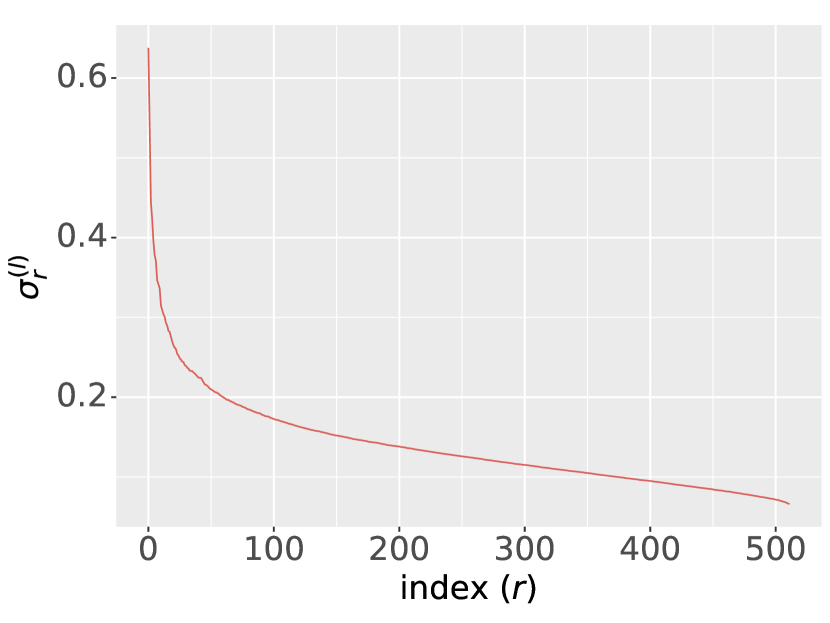
(a) singular values $S^{(l)}$

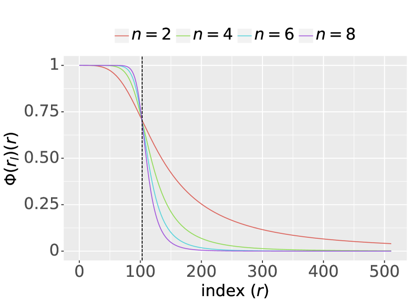
(b) $\Phi(r_{l})$ w/ various orders

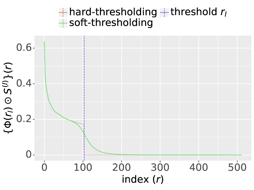
(c) thresholding by $\Phi(r_{l})\odot S^{(l)}$

Figure 2: Differentiable thresholding with a high-order normalized Butterworth kernel $\Phi(r_{l})$. The $S^{(l)}$ is in the $14$-th layer of a pre-trained resnet18 on ImageNet. The cut-off rank $r_{l}$ is $103$.

3.1 Differentiable relaxation

Equation (3) is not differentiable with respect to $r$. Solving the discrete combinatorial optimization problem in Equation (3) often entails iterative algorithms, e.g. evolutionary algorithms (EA) and integer programming (IP) (Bartz-Beielstein et al., 2014; Mazyavkina et al., 2021; Wolsey, 2020). Nevertheless, the huge discrete search spaces remain a significant hurdle. For instance, the number of possible combinations of low-rank adapter sizes in a resnet50 is above $10^{18}$.

To enable efficient optimization, firstly, we relax the $r$ in Equation (3) from discrete integers to continuous values. Secondly, we differentiably parameterize the operations of choosing $r$, by using a high-order normalized Butterworth kernel. With these endeavors, Equation (3) is differentiable with respect to $r$. We are able to use standard gradient descent algorithms to efficiently optimize (e.g. SGD and Adam).

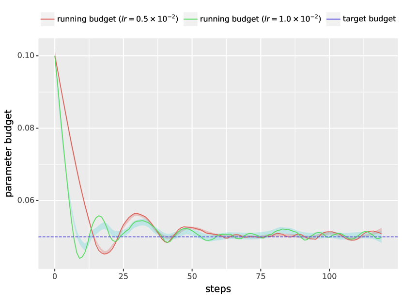
(a) running budget ($\omega^{T}r$)

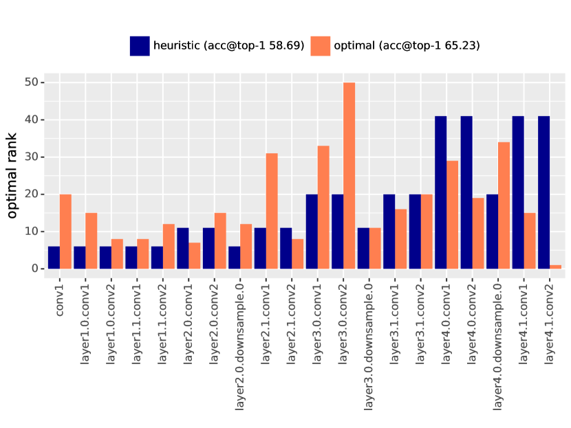
(b) solution

Figure 3: Optimization iterations and solution. The experiments are with resnet18 pre-trained on ImageNet.

3.2 Parameterized differentiable thresholding

Hard thresholding. Suppose $S^{(l)}$ is the singular value matrix of $[\![\Delta W^{(l)}]\!]_{n}$. Suppose $S_{r_{l}}^{(l)}$ chooses the $r_{l}$ largest values of $S^{(l)}$:

$$S^{(l)}=diag(\sigma_{1}^{(1)},\cdots,\sigma_{R_{l}}^{(l)})\quad S_{r_{l}}^{(l)}=diag(\sigma_{1}^{(1)},\cdots,\sigma_{r_{l}}^{(l)},0,\cdots,0)\quad 0\leq r_{l}\leq R_{l}.$$ (8)

Formally, choosing the $r_{l}$ can be formulated as the Hadamard product (i.e. element-wise product) of a thresholding mask matrix $\Phi^{*}(r_{l})$ and $S^{(l)}$ in that:

$$S_{r_{l}}^{(l)}=\Phi^{*}(r_{l})\odot S^{(l)}\qquad\Phi^{*}(r_{l})=diag(\underbrace{1,\cdots,1}_{r_{l}~{}\mathrm{ones}},\underbrace{0,\cdots,0}_{R_{l}-r_{l}~{}\text{zeros}}).$$ (9)

We refer to Equation (9) as hard-thresholding, which is not differentiable with respect to $r$.

Soft thresholding. We differentiably approximate the hard-thresholding with a high-order normalized Butterworth kernel (NBK) (Butterworth et al., 1930). An $k$-order NBK with a cut-off rank $r_{l}$ is a vector map $\Phi(r_{l}):r_{l}\mapsto[0,1]^{R_{l}}$ defined by:

$$\Phi(r_{l}):=\left(\frac{1}{\sqrt{1+(\frac{r}{r_{l}})^{2k}}}\right)_{r=1}^{R_{l}}\qquad r_{l}\ll R_{l}$$ (10)

where $n$ is the order. Figure 2(a) shows an example of $S^{(l)}$. Figure 2(b) shows an example of NBK. Figure 2(c) shows the results of the differentiable thresholding with NBK.

Converting residual operator to low-rank operator. In the $l$-th layer, we differentiably convert a high-rank residual operator $\Delta[\![W^{(l)}]\!]_{n}$ into a low-rank operator $B_{r_{l}}^{(l)}\circledast A_{r_{l}}^{(l)}$ with rank $r_{l}$, by using Equation (10):

$$\Delta[\![W^{(l)}]\!]_{n} \approx B_{r_{l}}^{(l)}\circledast A_{r_{l}}^{(l)}$$ (11)

$$\approx({U^{(l)}}[\Phi(r_{l})\odot{S^{(l)}}^{\frac{1}{2}}])_{[1,n\times k_{1}\times k_{2}]}\circledast([\Phi(r_{l})\odot{S^{(l)}}^{\frac{1}{2}}]{V^{(l)}}^{T})_{[1,r_{l}\times 1\times 1]}.$$ (12)

which is differentiable with respect to $r_{l}$.

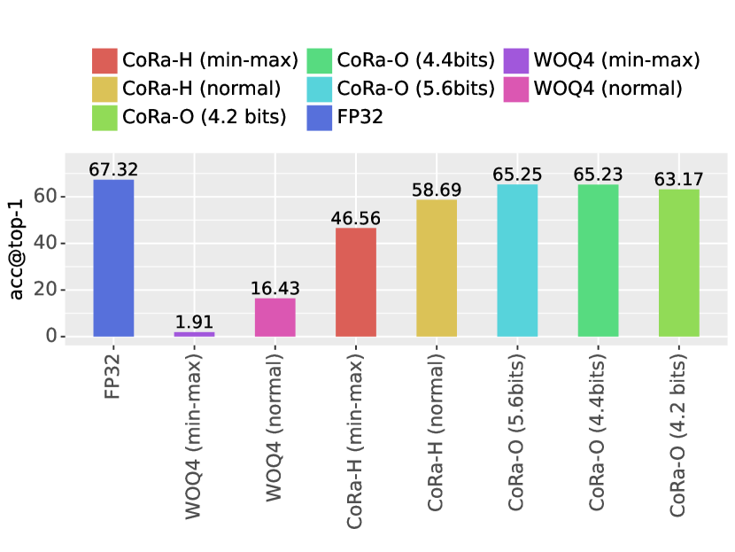
Figure 4: Ablation study on ImageNet with resnet18. CoRa-H: Heuristic ranks. CoRa-O: Optimal ranks.

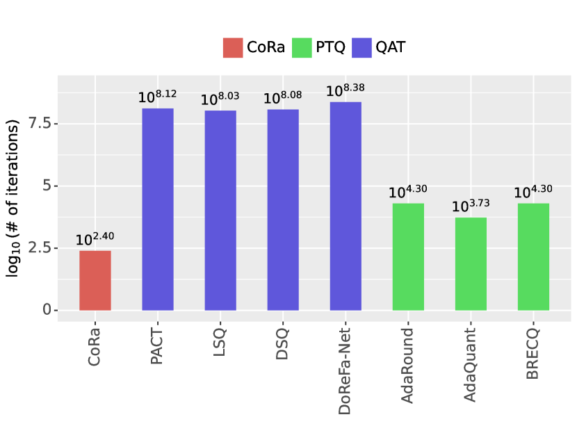
Figure 5: Optimization efficiency on ImageNet. Results are in a logarithmic scale.

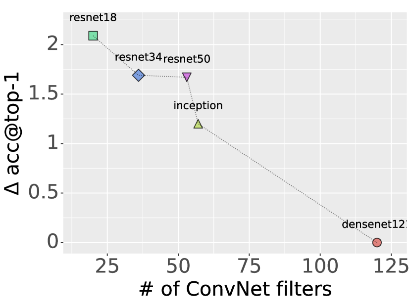
Figure 6: Performance scalability with respect to ConvNet sizes.

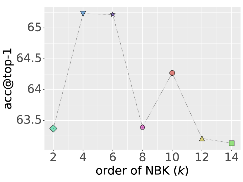
Figure 7: Sensitivity of the order $k$.

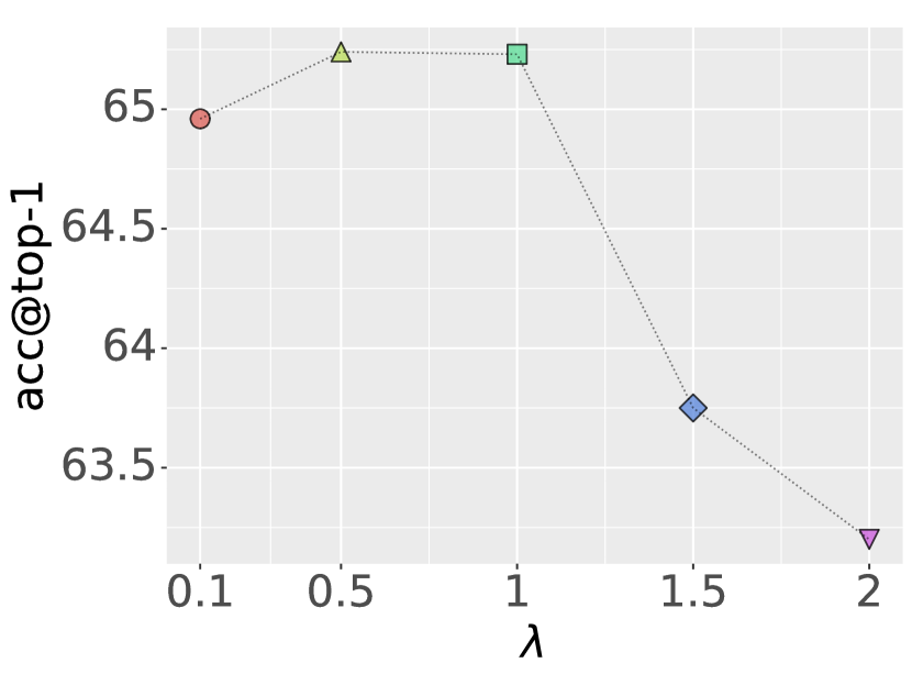
Figure 8: Sensitivity of $\lambda$.

3.3 Neural combinatorial optimization

By combining Equation (3) and Equation (7), the optimization loss is:

$$\mathcal{L}({\color[rgb]{0,0,1}{\bf\it r}}):=\mathop{\mathbb{missing}}{E}_{\langle x,y\rangle\sim\langle\mathcal{X},\mathcal{Y}\rangle}\left\{-\log Q(y|x;\widetilde{{\bf\it\theta}},{\bf\it\phi},{\color[rgb]{0,0,1}{\bf\it r}})+\lambda\cdot\exp{ReLU({\bf\it\omega}^{T}{\color[rgb]{0,0,1}{\bf\it r}}-b)}\right\}.$$ (13)

The optimal $r=\{r_{1},\cdots,r_{L}\}$ are found using gradient descent optimizers, e.g.SGD and Adam.

Heuristic choice of ranks. This method serves as a baseline. The $r_{l}$ is heuristically chosen as $r_{l}=\lfloor b\cdot R_{l}\rfloor$, proportionally assigning the $l$-th layer rank according to the budget $b$. For example, suppose the maximum rank at the $l$-th layer is $512$ and budget $b$ is set to $5\%$, the heuristic $r_{l}$ is chosen as $\lfloor 512\times 0.05\rfloor=25$.

Intriguing observation. Figure 3(a) shows the running budget $\omega^{T}r$ during the optimization. Figure 3(b) shows an example of the solution on a resnet18 on ImageNet. Our analysis in terms of the solutions from a variety of ConvNets suggests that: The heuristic choices often overstate the importance of middle to last layers; conversely, optimal solutions underscore the importance of beginning to middle layers.

3.4 Tricks for stable optimization

Stable optimization for the proposed neural combinatorial optimization in Section 3.3 is challenging. We adopt several tricks to numerically stabilize the optimization process.

• Gradient clipping. To stabilize the optimization, the solver clips the gradients into the range of $[-0.2,0.2]$.

• Adaptive gradient. Equation (7) gives non-linear gradients with respect to ranks. Smaller ranks have smaller gradients towards zero, while larger ranks have larger gradients. We believe this design favors the stabilization of optimization.

• Solution clamping. The solver clamps the ranges of the solutions after every gradient update, guaranteeing that the rank is not less than $1$ and not greater than the limit $R_{l}$.

• Anomaly reassignment. The solver detects numerical anomalies. If a NaN rank value is detected, it is replaced with rank $1$.

4 Experiments

We conduct experiments from five aspects: (1) ablation study (Section 4.1), (2) comparing with state-of-the-art QAT and PTQ baselines (Section 4.2), (3) extensive evaluation (Section 4.3), (4) performance scalability with respect to model sizes (Section 4.4) and (5) hyper-parameter sensitivity (Section 4.5).

Reproducibility. We sample $1600$ images from the ImageNet validation set as our calibration set while using the remainder as our validation set. We use normal clipping with $k=4.0$ to quantize the main network and min-max clipping to quantize adapters. The order $n$ of NBK is set to $4.0$. The penalty coefficient $\lambda$ is set to $1$. The batch size is $32$. The target budget $b$ is set to $5\%$, which results in a $1.25\%$ increase in memory footprint with $8$-bit quantization for low-rank adapters. The optimizer is Adam without weight decay. The learning rate is set to $0.01$. We use a maximum $250$ iterations for all experiments.

Testbed. All experimental results, including the measured results of floating-point reference accuracy, are conducted on the M2 chip of a MacBook Air, equipped with a GPU of size 24 GiB. Due to the choice of the validation set, in tandem with the random seed and the hardware acceleration implementation in the testbed, the results of reference accuracy are slightly lower compared to the results from pytorch. However, this does not affect the results, we obtain using pytorch, for a fair comparisons with baselines. We report the results that we measured on our own testbed rather than using the results from the literature.

Equivalent quantization bit-width. Let $n$ and $m$ be the quantization bit-widths of the main network and adapters. The equivalent quantization bit-width is given as: $n+m\cdot b$. For example, suppose $n=4$, $m=8$ and $b=5\%$, the equivalent quantization bit-width is $4.4$-bits. The proof is provided in Appendix E.

Table 1: Top-1 accuracy comparison of low-bit quantization. We use marker $\times$ to indicate that the results are not available.

Model	bits	FP32	CoRa	QAT Baselines				PTQ Baselines
				PACT	LSQ	DSQ	DoReFa-Net	AdaRound	AdaQuant	BRECQ
resnet18	4	67.32	65.23	66.08	67.89	66.99	65.99	65.08	65.18	66.96
resnet50		74.52	72.85	$\times$	73.84	73.39	$\times$	72.81	72.80	73.88
resnet18	3		64.50	65.31	66.13	$\times$	$\times$	64.47	55.04	66.12
resnet50			72.81	$\times$	$\times$	$\times$	$\times$	71.06	65.43	70.87
# of iterations		$10^{8.38}$	$\leq 10^{2.40}$	$10^{8.12}$	$10^{8.03}$	$10^{8.08}$	$10^{8.38}$	$10^{4.30}$	$10^{3.73}$	$10^{4.30}$
training size		$1.2M$	$1600$	$1.2M$	$1.2M$	$1.2M$	$1.2M$	2048	1000	1024

4.1 Ablation study

We conduct ablation experiments to show the design considerations in: (1) normal clipping is better than min-max clipping, (2) the results with optimal ranks outperform the results with heuristic choices, and (3) quantizing residual adapters with $8$-bits does not affect performance. The results are shown in Figure 8.

Intriguingly, we can quantize adapters while the performance remains almost unchanged. This can significantly reduce the amount of extra parameters which are used to retain residual knowledge.

4.2 Comparing with baselines

We compare our method against both state-of-the-art QAT and PTQ baselines. We choose four QAT baselines: PACT (Choi et al., 2018), LSQ (Esser et al., 2019), DSQ (Gong et al., 2019), and DoReFa-Net (Zhou et al., 2016). We choose three PTQ baselines: AdaRound (Nagel et al., 2020), AdaQuant (Hubara et al., 2020), and BRECQ (Li et al., 2021b). We quantize the resnet18 and resnet50 (pre-trained on ImageNet) with $4$-bits and $3$-bits quantization.

Top-1 accuracy. Our results achieve comparable performance against the baselines. The results are shown in Table 1. Optimization efficiency. Our method is more efficient by many orders of magnitude than state-of-the-art baselines. The results are shown in Figure 8 and Table 1. Notably, our method uses only $250$ iterations with very minimum extra parameter cost. We have established a new state-of-the-art in terms of optimization efficiency.

4.3 Extensive evaluation

We show the results of extensive performance evaluation over multiple image classifiers pre-trained on ImageNet in Figure 9. Our results achieve comparable performance against the floating-point reference models with the differences within $2.5\%$. The full solutions are provided in Appendix F.

4.4 Performance scalability

Figure 8 shows the performance scalability of CoRa with respect to model sizes, which are assessed by the numbers of filters. The result shows that the top-1 accuracy difference to floating-point models decreases with respect to the number of filters in models.

4.5 Hyper-parameter sensitivity

There are two hyper-parameters: the order $n$ of the NBK in Equation (10) and the $\lambda$ in the loss function. We empirically investigate how their choices affect performance. The experiments are on a resnet18 pre-trained on ImageNet. Figure 8 shows that the NBK order $k=4$ achieves best performance. Figure 8 shows that $\lambda$ achieves best performance between $0.5$ and $1$. It is notable that $k$ and $\lambda$ are model-dependent.

5 Related work

Low-rank convolutional operator approximation. Low-rank approximation of convolutional operators is promising in accelerating the computations (Li et al., 2021a). However, convolution operations are not matrix multiplications. Conventional low-rank approximation, e.g. LoRa (Hu et al., 2021) and QLoRa Dettmers et al. (2024), fails to approximate convolutional operators. Relatively few works in the literature have explored this problem. Denton et al. decompose filters into the outer product of three rank-$1$ filters by optimization (Denton et al., 2014). Rigamonti et al. use rank-$1$ filters to approximate convolutional filters by learning (Rigamonti et al., 2013). Jaderberg et al. reconstruct low-rank filters with optimization, by exploiting the significant redundancy across multiple channels and filters (Jaderberg et al., 2014). A recent work, Conv-LoRA, approximates filters with the composed convolutions of two filters for low-rank fine-tuning on ConvNets (Zhong et al., 2024). However, Conv-LoRA does not solve the problem of converting existing operators to low-rank operators without training. Previous works need to reconstruct low-rank filters by learning, thus they do not satisfy our needs. CoRa uses Theorem 1 to convert existing residual operators into low-rank operators without training.

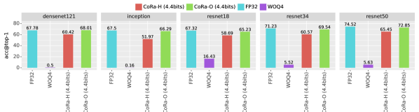
Figure 9: Top-1 accuracy of multiple vision architectures on ImageNet with $4$-bit quantization.

6 Future work

CoRa introduces a novel paradigm in low-bit quantization and demonstrates significant optimization efficiency, with a new state-of-the-art result, as shown by our experiments compared to baselines. This paper exclusively investigates this paradigm on ConvNets. Future research will aim to explore this paradigm further from three aspects: (1) enhancing the performance of existing quantization methods (e.g. QAT and PQT) by reclaiming the residual knowledge using CoRa; (2) extending this paradigm to architectures beyond ConvNets, such as transformers; and (3) broadening the scope to more diverse tasks, including large vision models (LVMs) and large language models (LLMs).

7 Conclusions

We explore a novel paradigm, in optimal low-bit quantization, differing from existing state-of-the-art methods, by re-framing the problem as an architecture search problem, of optimally reclaiming quantization residual knowledge. Thanks to significantly smaller search spaces of adapters, our method is more efficient yet achieves comparable performance against state-of-the-art baselines. CoRa has established a new state-of-the-art in terms of the optimization efficiency.

Appendix

Appendix A Uniform quantization

We formally introduce uniform quantization, which refers to the integer representations of floating-point tensors by taking the quantization intervals uniformly (Gholami et al., 2022; Guo, 2018).

Suppose:

$$\lfloor\cdot\rceil:\mathbb{R}^{I_{1}\times I_{2}\times\cdots\times I_{N}}\mapsto\mathbb{Z}^{I_{1}\times I_{2}\times\cdots\times I_{N}}$$ (14)

is an element-wise rounding operator in tensor space such as $round(\cdot)$, $floor(\cdot)$ or $ceil(\cdot)$ in pytorch (Ketkar et al., 2021).

Quantization operator. Suppose:

$$[\![\cdot]\!]_{n}:\mathbb{R}^{I_{1}\times I_{2}\times\cdots\times I_{N}}\mapsto\mathbb{Z}^{I_{1}\times I_{2}\times\cdots\times I_{N}}$$ (15)

is a $n$-bit quantization operator which sends tensors from floating-point representations to $n$-bit integer representations.

De-quantization operator. We define the de-quantization operator as:

$$[\![\cdot]\!]_{n}^{-1}:\mathbb{Z}^{I_{1}\times I_{2}\times\cdots\times I_{N}}\mapsto\mathbb{R}^{I_{1}\times I_{2}\times\cdots\times I_{N}}.$$ (16)

Let ${\bf\it x}\in\mathbb{R}^{I_{1}\times I_{2}\times\cdots\times I_{N}}$ be some floating-point tensor. Let $[\alpha,\beta]\subset\mathbb{R}$ be the quantization representation range (i.e. quantization clipping range) where $\alpha,\beta\in\mathbb{R}$. Choosing the clipping range constant $[\alpha,\beta]$ is often referred as ‘calibration’ (Gholami et al., 2022). Let $s\in\mathbb{R}$ be some scale constant determined by quantization bit-width and representation range $[\alpha,\beta]$:

$$s(n;\alpha;\beta)=\frac{\alpha-\beta}{2^{n}-1}.$$ (17)

Suppose $z\in\mathbb{Z}$ denotes the integer representation zero point (i.e. quantization bias), the quantization operator $[\![\cdot]\!]_{n}$ can be formulated as:

$${\bf\it x}^{*}=[\![{\bf\it x}]\!]_{n}\stackrel{{\scriptstyle def}}{{=}}\lfloor\frac{{\bf\it x}}{s(n;\alpha;\beta)}\rceil-z$$ (18)

which represents ${\bf\it x}$ into the range:

$$[\lfloor\frac{\alpha}{s(n;\alpha,\beta)}\rceil-z,\lfloor\frac{\beta}{s(n;\alpha,\beta)}\rceil-z]\subset\mathbb{Z}.$$ (19)

The choices of $z$ determine two schemes for uniform quantization: (1) Symmetric quantization scheme and (2) asymmetric quantization scheme (i.e. affine quantization) (Gholami et al., 2022; Jacob et al., 2018; Krishnamoorthi, 2018).

For example, the scheme $z:=\frac{\alpha}{s(n;\alpha,\beta)}$ is dubbed as ‘asymmetric quantization scheme’ or ‘affine quantization scheme’ where the floating-point representation zero-point is mapped to the bias $z$. The scheme $z:=0$ is dubbed as ‘symmetric quantization scheme’ where the floating-point representation zero-point is mapped to zero.

Accordingly, the de-quantization operator $[\![\cdot]\!]_{n}^{-1}$ can be formulated as:

$${\bf\it x}=[\![{\bf\it x}^{*}]\!]_{n}^{-1}\stackrel{{\scriptstyle def}}{{=}}s(n;\alpha,\beta)\cdot({\bf\it x}^{*}+z).$$ (20)

Appendix B Mode-$n$ tensor product

Let $Z\in\mathbb{R}^{I_{1}\times I_{2}\times\cdots\times I_{N}}$ be a $N$-order tensor where $I_{i}$ denotes the $i$-th dimension size. A ‘fiber’ refers to the vector created by fixing $N-1$ dimensions. A ‘slice’ refers to the matrix created by fixing $N-2$ dimensions.

The mode-$n$ matricization of tensor $Z$ is also known as tensor ‘unfolding’. For example, a tensor with shape $8\times 16\times 3\times 3$ can be unfolded into a matrix with shape $8\times 144$. The mode-$n$ matricization of tensor $Z$ is denoted as $Z_{(n)}$ by arranging the mode-$n$ fibres of $Z$ as columns. The mode-$n$ product is known as tensor-matrix product. The mode-$n$ product of tensor $Z$ and matrix $Y\in\mathbb{R}^{J\times I_{n}}$ is defined as $Z\times_{n}Y\stackrel{{\scriptstyle def}}{{=}}YZ_{(n)}$.

Accordingly, we also define the inverse mode-$n$ tensorization (i.e. ‘folding’) as the inverse operation and denote it as $Z_{[n,J_{1}\times J_{2}\times\cdots\times J_{K}]}$ where $J_{1}\times J_{2}\times\cdots\times J_{K}$ denotes the folding dimensions of the unfolded dimensions in $Z_{(n)}$. Readers can refer to the literature (Kolda and Bader, 2009) for details.

Appendix C Proof: Residual convolutional representation

We aim to prove:

$$W\circledast{\bf\it x}=[\![W]\!]_{n}\circledast{\bf\it x}+\underbrace{B\circledast A}_{\mathrm{residual~{}operator}}\circledast{\bf\it x}$$ (21)

as stated in Theorem 1.

However, the convolutional operations are not matrix multiplications. We can not directly use the results such as singular value decomposition (SVD). Strictly proving the Theorem 1 demands some efforts. We use the knowledge from tensor algebra to show that Theorem 1 holds.

Definition 1 (Unfolding operator).

Let:

$$\mathbb{T}(k_{1}\times k_{2},s_{1}\times s_{2}):\mathbb{R}^{n\times w\times h}\mapsto\mathbb{R}^{n\cdot k_{1}\cdot k_{2}\times w^{\prime}\times h^{\prime}}$$ (22)

be the ‘unfolding’ operation which arranges some input with shape ‘$n\times w\times h$’ to shape ‘$n\cdot k_{1}\cdot k_{2}\times w^{\prime}\times h$’ for convolution operation with respect to kernel size $k_{1}\times k_{2}$ and stride size $s_{1}\times s_{2}$. In particular, if the stride size is $1\times 1$, we simplify the notation as:

$$\mathbb{T}(k_{1}\times k_{2}).$$ (23)

Suppose ${\bf\it x}\in\mathbb{R}^{n\times w\times h}$. For example, the operator with stride $s_{1}\times s_{2}$ and no padding is defined by:

$$\mathbb{T}(k_{1}\times k_{2},s_{1}\times s_{2})({\bf\it x})(c,u,v):={\bf\it x}(c\mod{(n\cdot k_{1}\cdot k_{2})},\lfloor\frac{u}{s_{1}}\rfloor,\lfloor\frac{v}{s_{2}}\rfloor)$$ (24)

where $c,u$ and $v$ are indices. Clearly:

$$\mathbb{T}(1\times 1)({\bf\it x})\equiv{\bf\it x}$$ (25)

holds true as a particular case. Readers can refer to the implementation of the operation unfold in pytorch.

Lemma 2 (Tensor mode-$n$ product factorization).

Let $Z\in\mathbb{R}^{I_{1}\times I_{2}\times\cdots\times I_{N}}$ be some tensor. Let $A\in\mathbb{R}^{R\times I_{n}}$ and $B\in\mathbb{R}^{J\times R}$ be matrices. Below identity holds:

$$Z\times_{n}A\times_{n}B\equiv Z\times_{n}(BA).$$ (26)

Readers can refer to literature (Kolda and Bader, 2009) for the proof.

Lemma 3 (Convolution mode-$n$ representation).

Let $W\in\mathbb{R}^{m\times n\times k_{1}\times k_{1}}$ be the weights of some ‘$k_{1}\times k_{1}$’ 2D convolutional operator where $m$ denotes output channels and $n$ denotes input channels. Let ${\bf\it x}\in\mathbb{R}^{n\times w\times h}$ be some input with size $w\times h$ and channels $n$. According to the definition of 2D convolution, the convolution $W\circledast{\bf\it x}$ can be represented as:

$$W\circledast{\bf\it x}=\underbrace{\mathbb{T}(k_{1}\times k_{2})({\bf\it x})}_{n\cdot k_{1}\cdot k_{2}\times w^{\prime}\times h^{\prime}}\times_{1}W_{(1)}.$$ (27)

Theorem 4 (Convolution factorization).

Let $Z\in\mathbb{R}^{m\times n\times k_{1}\times k_{2}}$ be the weights of some 2D convolutional operator. Suppose:

$$Z_{(1)}=B_{(1)}A_{(1)}\in\mathbb{R}^{m\times n\cdot k_{1}\cdot k_{2}}$$ (28)

where $A\in\mathbb{R}^{d\times n\times k_{1}\times k_{2}}$ and $B\in\mathbb{R}^{m\times d\times 1\times 1}$ are the weights of two convolutional operators with kernel sizes ‘$k_{1}\times k_{1}$’ and ‘$1\times 1$’ respectively. Let ${\bf\it x}\in\mathbb{R}^{n\times w\times h}$ be some input. Using Lemma 3 and Lemma 2:

$$Z\circledast{\bf\it x} =\mathbb{T}(k_{1}\times k_{2})({\bf\it x})\times_{1}Z_{(1)}$$ (29)

$$=\mathbb{T}(k_{1}\times k_{2})({\bf\it x})\times_{1}(B_{(1)}A_{(1)})$$ (30)

$$=\mathbb{T}(k_{1}\times k_{2})({\bf\it x})\times_{1}A_{(1)}\times_{1}B_{(1)}$$ (31)

$$=(A\circledast{\bf\it x})\times_{1}B_{(1)}$$ (32)

$$=\mathbb{T}(1\times 1)(A\circledast{\bf\it x})B_{(1)}$$ (33)

$$=B\circledast A\circledast{\bf\it x}.$$ (34)

Corollary 5 (Convolutional singular value decomposition).

Suppose:

$$Z_{(1)}=USV^{T}=US^{\frac{1}{2}}(S^{\frac{1}{2}}V)^{T}$$ (35)

where:

$$S^{\frac{1}{2}}\odot S^{\frac{1}{2}}=S.$$ (36)

Set:

$$B_{(1)}:=US^{\frac{1}{2}}$$ (37)

and:

$$A_{(1)}:=(S^{\frac{1}{2}}V)^{T}.$$ (38)

Using Theorem 4:

$$Z\circledast{\bf\it x}=(US^{\frac{1}{2}})_{[1,d\times 1\times 1]}\circledast(S^{\frac{1}{2}}V)^{T}_{[1,n\times k_{1}\times k_{2}]}\circledast{\bf\it x}.$$ (39)

Proof.

We now show that the Theorem 1 strictly holds by using Theorem 4 and Corollary 5. Suppose $W\in\mathbb{R}^{m\times n\times k_{1}\times k_{2}}$ be the weights of some convolutional operator. Set:

$$Z:=\Delta[\![W]\!]_{n}\in\mathbb{R}^{m\times n\times k_{1}\times k_{2}}.$$ (40)

Convolutional operators are linear operators. The convolution quantization residual representation is:

$$W\circledast{\bf\it x} =[\![W]\!]_{n}\circledast{\bf\it x}+\Delta[\![W]\!]_{n}\circledast{\bf\it x}$$ (41)

$$=[\![W]\!]_{n}\circledast{\bf\it x}+(US^{\frac{1}{2}})_{[1,d\times 1\times 1]}\circledast(S^{\frac{1}{2}}V)^{T}_{[1,n\times k_{1}\times k_{2}]}\circledast{\bf\it x}.$$ (42)

There is nothing to do. Theorem 1 holds as demonstrated. ∎

Appendix D Rank normalization coefficients

Suppose a model with $L$ convolutional filters. Suppose the $l$-th layer has parameter size $\Theta_{l}$. Suppose the adaptation of the $i$-th layer has parameters $\Xi_{i}$. The maximum parameter size of the $l$-th adapter is $\Theta_{l}$.

The overall size of the adapters is given by:

$$\frac{r_{l}}{R_{l}}\cdot\Theta_{l}.$$ (43)

Normalizing with respect to the overall model size:

$$\sum\limits_{i=1}^{L}\Theta_{i}.$$ (44)

Thus, the running budget is:

$$\frac{r_{l}}{R_{l}}\cdot\Theta_{l}\cdot\frac{1}{\sum\limits_{i=1}^{L}\Theta_{i}}\leq b.$$ (45)

Set:

$$\omega_{l}=\frac{1}{R_{l}}\cdot\frac{\Theta_{l}}{\sum\limits_{i=1}^{L}\Theta_{i}}$$ (46)

which is referred as $l$-th layer rank normalization coefficient.

Appendix E Equivalent quantization bit-width

Suppose the $l$-th layer parameter size $\Theta_{l}$. The the $l$-th layer adapter size is:

$$\frac{r_{l}}{R_{l}}\cdot\Theta_{l}.$$ (47)

The equivalent quantization bit-width $\xi$ is:

$$\frac{\xi}{32}=\frac{\frac{n}{32}\cdot\sum\limits_{i=1}^{L}\Theta_{i}+\frac{m}{32}\cdot\sum\limits_{i=1}^{L}\frac{r_{l}}{R_{l}}\cdot\Theta_{i}}{\sum\limits_{i=1}^{L}\Theta_{i}}.$$ (48)

Simplifying the Equation (48):

$$\xi=n+m\cdot b.$$ (49)

Appendix F Full solutions

We provide full solutions for all experimental models.

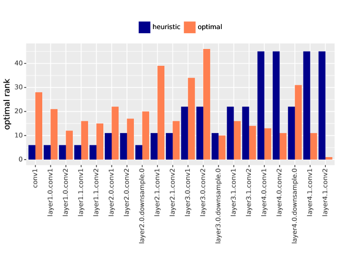
Figure 10: Solution for resnet18.

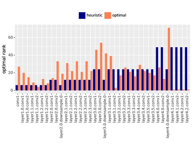
Figure 11: Solution for resnet34.

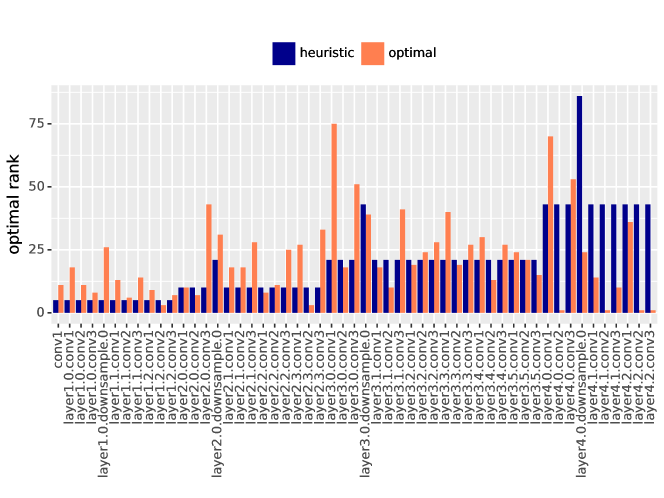
Figure 12: Solution for resnet50.

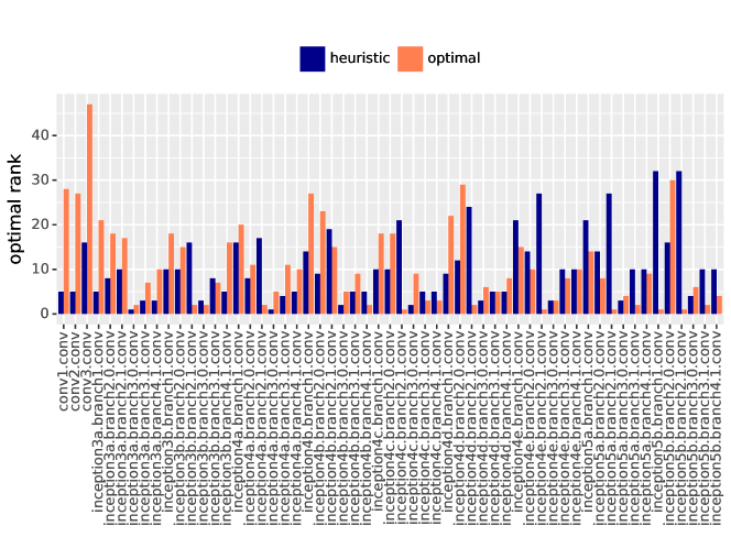
Figure 13: Solution for inception.

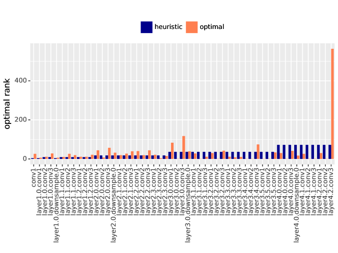
Figure 14: Solution for wide_resnet50_2.

References

- Li et al. (2021a) Zewen Li, Fan Liu, Wenjie Yang, Shouheng Peng, and Jun Zhou. A survey of convolutional neural networks: analysis, applications, and prospects. IEEE transactions on neural networks and learning systems, 2021a.
- Awais et al. (2023) Muhammad Awais, Muzammal Naseer, Salman Khan, Rao Muhammad Anwer, Hisham Cholakkal, Mubarak Shah, Ming-Hsuan Yang, and Fahad Shahbaz Khan. Foundational models defining a new era in vision: A survey and outlook. arXiv preprint arXiv:2307.13721, 2023.
- Wang and Wu (2024) Zihao Wang and Lei Wu. Theoretical analysis of the inductive biases in deep convolutional networks. Advances in Neural Information Processing Systems, 36, 2024.
- d’Ascoli et al. (2019) Stéphane d’Ascoli, Levent Sagun, Giulio Biroli, and Joan Bruna. Finding the needle in the haystack with convolutions: on the benefits of architectural bias. Advances in Neural Information Processing Systems, 32, 2019.
- Hermann et al. (2020) Katherine Hermann, Ting Chen, and Simon Kornblith. The origins and prevalence of texture bias in convolutional neural networks. Advances in Neural Information Processing Systems, 33:19000–19015, 2020.
- Maurício et al. (2023) José Maurício, Inês Domingues, and Jorge Bernardino. Comparing vision transformers and convolutional neural networks for image classification: A literature review. Applied Sciences, 13(9):5521, 2023.
- Han et al. (2015) Song Han, Huizi Mao, and William J Dally. Deep compression: Compressing deep neural networks with pruning, trained quantization and huffman coding. arXiv preprint arXiv:1510.00149, 2015.
- Neill (2020) James O’ Neill. An overview of neural network compression. arXiv preprint arXiv:2006.03669, 2020.
- Mishra et al. (2020) Rahul Mishra, Hari Prabhat Gupta, and Tanima Dutta. A survey on deep neural network compression: Challenges, overview, and solutions. arXiv preprint arXiv:2010.03954, 2020.
- Liang et al. (2021) Tailin Liang, John Glossner, Lei Wang, Shaobo Shi, and Xiaotong Zhang. Pruning and quantization for deep neural network acceleration: A survey. Neurocomputing, 461:370–403, 2021.
- Choukroun et al. (2019) Yoni Choukroun, Eli Kravchik, Fan Yang, and Pavel Kisilev. Low-bit quantization of neural networks for efficient inference. In 2019 IEEE/CVF International Conference on Computer Vision Workshop (ICCVW), pages 3009–3018. IEEE, 2019.
- Gholami et al. (2022) Amir Gholami, Sehoon Kim, Zhen Dong, Zhewei Yao, Michael W Mahoney, and Kurt Keutzer. A survey of quantization methods for efficient neural network inference. In Low-Power Computer Vision, pages 291–326. Chapman and Hall/CRC, 2022.
- Li et al. (2023) Zhuo Li, Hengyi Li, and Lin Meng. Model compression for deep neural networks: A survey. Computers, 12(3):60, 2023.
- Deng et al. (2009) Jia Deng, Wei Dong, Richard Socher, Li-Jia Li, Kai Li, and Li Fei-Fei. Imagenet: A large-scale hierarchical image database. In 2009 IEEE conference on computer vision and pattern recognition, pages 248–255. Ieee, 2009.
- Nagel et al. (2021) Markus Nagel, Marios Fournarakis, Rana Ali Amjad, Yelysei Bondarenko, Mart Van Baalen, and Tijmen Blankevoort. A white paper on neural network quantization. arXiv preprint arXiv:2106.08295, 2021.
- Nagel et al. (2020) Markus Nagel, Rana Ali Amjad, Mart Van Baalen, Christos Louizos, and Tijmen Blankevoort. Up or down? adaptive rounding for post-training quantization. In International Conference on Machine Learning, pages 7197–7206. PMLR, 2020.
- Guo (2018) Yunhui Guo. A survey on methods and theories of quantized neural networks. arXiv preprint arXiv:1808.04752, 2018.
- Choi et al. (2018) Jungwook Choi, Zhuo Wang, Swagath Venkataramani, Pierce I-Jen Chuang, Vijayalakshmi Srinivasan, and Kailash Gopalakrishnan. Pact: Parameterized clipping activation for quantized neural networks. arXiv preprint arXiv:1805.06085, 2018.
- Nagel et al. (2022) Markus Nagel, Marios Fournarakis, Yelysei Bondarenko, and Tijmen Blankevoort. Overcoming oscillations in quantization-aware training. In International Conference on Machine Learning, pages 16318–16330. PMLR, 2022.
- Liu and Mattina (2019) Zhi-Gang Liu and Matthew Mattina. Learning low-precision neural networks without straight-through estimator (ste). arXiv preprint arXiv:1903.01061, 2019.
- Esser et al. (2019) Steven K Esser, Jeffrey L McKinstry, Deepika Bablani, Rathinakumar Appuswamy, and Dharmendra S Modha. Learned step size quantization. arXiv preprint arXiv:1902.08153, 2019.
- Li et al. (2021b) Yuhang Li, Ruihao Gong, Xu Tan, Yang Yang, Peng Hu, Qi Zhang, Fengwei Yu, Wei Wang, and Shi Gu. Brecq: Pushing the limit of post-training quantization by block reconstruction. arXiv preprint arXiv:2102.05426, 2021b.
- He et al. (2016) Kaiming He, Xiangyu Zhang, Shaoqing Ren, and Jian Sun. Deep residual learning for image recognition. In Proceedings of the IEEE conference on computer vision and pattern recognition, pages 770–778, 2016.
- Hu et al. (2021) Edward J Hu, Yelong Shen, Phillip Wallis, Zeyuan Allen-Zhu, Yuanzhi Li, Shean Wang, Lu Wang, and Weizhu Chen. Lora: Low-rank adaptation of large language models. arXiv preprint arXiv:2106.09685, 2021.
- Zhang et al. (2015) Xiangyu Zhang, Jianhua Zou, Kaiming He, and Jian Sun. Accelerating very deep convolutional networks for classification and detection. IEEE transactions on pattern analysis and machine intelligence, 38(10):1943–1955, 2015.
- Yang et al. (2020) Huanrui Yang, Minxue Tang, Wei Wen, Feng Yan, Daniel Hu, Ang Li, Hai Li, and Yiran Chen. Learning low-rank deep neural networks via singular vector orthogonality regularization and singular value sparsification. In Proceedings of the IEEE/CVF conference on computer vision and pattern recognition workshops, pages 678–679, 2020.
- Denton et al. (2014) Emily L Denton, Wojciech Zaremba, Joan Bruna, Yann LeCun, and Rob Fergus. Exploiting linear structure within convolutional networks for efficient evaluation. Advances in neural information processing systems, 27, 2014.
- Rigamonti et al. (2013) Roberto Rigamonti, Amos Sironi, Vincent Lepetit, and Pascal Fua. Learning separable filters. In Proceedings of the IEEE conference on computer vision and pattern recognition, pages 2754–2761, 2013.
- Jaderberg et al. (2014) Max Jaderberg, Andrea Vedaldi, and Andrew Zisserman. Speeding up convolutional neural networks with low rank expansions. arXiv preprint arXiv:1405.3866, 2014.
- Zhong et al. (2024) Zihan Zhong, Zhiqiang Tang, Tong He, Haoyang Fang, and Chun Yuan. Convolution meets lora: Parameter efficient finetuning for segment anything model. arXiv preprint arXiv:2401.17868, 2024.
- Kolda and Bader (2009) Tamara G Kolda and Brett W Bader. Tensor decompositions and applications. SIAM review, 51(3):455–500, 2009.
- Li et al. (2018) James Li, Jacob Bien, and Martin T Wells. rtensor: An r package for multidimensional array (tensor) unfolding, multiplication, and decomposition. Journal of Statistical Software, 87:1–31, 2018.
- Zhou et al. (2021) Jingkai Zhou, Varun Jampani, Zhixiong Pi, Qiong Liu, and Ming-Hsuan Yang. Decoupled dynamic filter networks. In Proceedings of the IEEE/CVF Conference on Computer Vision and Pattern Recognition, pages 6647–6656, 2021.
- Bartz-Beielstein et al. (2014) Thomas Bartz-Beielstein, Jürgen Branke, Jörn Mehnen, and Olaf Mersmann. Evolutionary algorithms. Wiley Interdisciplinary Reviews: Data Mining and Knowledge Discovery, 4(3):178–195, 2014.
- Mazyavkina et al. (2021) Nina Mazyavkina, Sergey Sviridov, Sergei Ivanov, and Evgeny Burnaev. Reinforcement learning for combinatorial optimization: A survey. Computers & Operations Research, 134:105400, 2021.
- Wolsey (2020) Laurence A Wolsey. Integer programming. John Wiley & Sons, 2020.
- Butterworth et al. (1930) Stephen Butterworth et al. On the theory of filter amplifiers. Wireless Engineer, 7(6):536–541, 1930.
- Gong et al. (2019) Ruihao Gong, Xianglong Liu, Shenghu Jiang, Tianxiang Li, Peng Hu, Jiazhen Lin, Fengwei Yu, and Junjie Yan. Differentiable soft quantization: Bridging full-precision and low-bit neural networks. In Proceedings of the IEEE/CVF international conference on computer vision, pages 4852–4861, 2019.
- Zhou et al. (2016) Shuchang Zhou, Yuxin Wu, Zekun Ni, Xinyu Zhou, He Wen, and Yuheng Zou. Dorefa-net: Training low bitwidth convolutional neural networks with low bitwidth gradients. arXiv preprint arXiv:1606.06160, 2016.
- Hubara et al. (2020) Itay Hubara, Yury Nahshan, Yair Hanani, Ron Banner, and Daniel Soudry. Improving post training neural quantization: Layer-wise calibration and integer programming. arXiv preprint arXiv:2006.10518, 2020.
- Dettmers et al. (2024) Tim Dettmers, Artidoro Pagnoni, Ari Holtzman, and Luke Zettlemoyer. Qlora: Efficient finetuning of quantized llms. Advances in Neural Information Processing Systems, 36, 2024.
- Ketkar et al. (2021) Nikhil Ketkar, Jojo Moolayil, Nikhil Ketkar, and Jojo Moolayil. Introduction to pytorch. Deep Learning with Python: Learn Best Practices of Deep Learning Models with PyTorch, pages 27–91, 2021.
- Jacob et al. (2018) Benoit Jacob, Skirmantas Kligys, Bo Chen, Menglong Zhu, Matthew Tang, Andrew Howard, Hartwig Adam, and Dmitry Kalenichenko. Quantization and training of neural networks for efficient integer-arithmetic-only inference. In Proceedings of the IEEE conference on computer vision and pattern recognition, pages 2704–2713, 2018.
- Krishnamoorthi (2018) Raghuraman Krishnamoorthi. Quantizing deep convolutional networks for efficient inference: A whitepaper. arXiv preprint arXiv:1806.08342, 2018.