A reference frame-based microgrid primary control for ensuring global convergence to a periodic orbit

Abstract

Electric power systems with growing penetration of renewable generation face problems of frequency oscillation and increased uncertainty as the operating point may veer close to instability. Traditionally the stability of these systems is studied either in terms of local stability or as an angle synchronization problem under the simplifying assumption that decouples the amplitude along with all dissipations. Without the simplifying assumption, however, the steady state being studied is basically a limit cycle with the convergence of its orbit in question. In this paper we present an analysis of the orbital stability of a microgrid integrating the proposed type of distributed generation controller, whose internal reference voltage arises from the rotation of the reference frame much like a rotating machine. We utilize the shifted passivity framework to prove that, with sufficient dissipation, such system is globally convergent to a nontrivial orbit. This is the first global stability result for the limit cycle of such system in the full state space, which provides new insight into the synchronization mechanism as well as how dissipation plays a role in the orbital stability. The proposed controller is verified with a test microgrid, demonstrating its stability and transient smoothness compared to the standard droop control.

, , ,

1 Introduction

Microgrids are considered key to achieving sustainability of power systems by transitioning from centrally operated power plants to distributed energy resources (DER). Microgrid primary control refers to the lower-level control that determines the transient dynamics under sudden load or generation changes. Besides the steady state characteristics, the primary control of ac microgrid is designed to maintain stability under large power disturbances while relying on minimum communication between DER units. The stability analysis of primary control is thus the basis of all microgrid functionalities, where the main problem is to find the optimal DER control scheme and parameters to ensure stability and transient smoothness for the microgrid.

A prerequisite for the stability of primary control is to allow flexibility in the DER power output so that the power disturbance can be shared in steady states. This steady state power sharing is usually provided by the droop characteristic of the control (droop control) where active and reactive power droop down relative to their nominal values depending on the frequency and voltage increases. Droop control can be roughly classified as either related to the swing equation [39, 11, 38] or virtual oscillators [43, 18]. Due to the variable frequency, the stability problem of droop control is more difficult than a set point tracking problem considered in [34, 45, 42].

The difficulty in analyzing the stability with droop control lies in the coexistence of rotational symmetry and the $n$-torus space where the phase angles live. Due to rotational symmetry, the motion of the system never converges along the symmetry, resulting in a symmetry-invariant orbit. The common approach in dealing with systems with continuous symmetry is to reduce dimensionality, i.e., to express the system in a set of transverse coordinates with respect to the symmetry [24, 3, 35]. In general, the reduced dynamics may be more complicated or the transverse state space may be pathological [10]. In the case of a microgrid, however, since its angle symmetry can be removed by switching to relative angles, the reduction approach works to some degree. The main issue is that the dissipation that needs to be checked for a candidate Lyapunov function cannot be obtained easily in transverse coordinates. For example, in [39, 11], the strategy is to find an energy function in the original coordinates, not necessarily bounded from below, but decreases monotonically along the motion, and then to check whether this function is convex at the equilibrium point that exists in the transverse coordinates, and hence local stability. They extend the traditional of energy function in the power engineering [8] and avoid the issue of expressing dissipation in the symmetry-invariant coordinates. The limitation of this approach is that the Lyapunov function cannot provide any information on the attractive set. To find dissipation in symmetry-invariant coordinates, however, one faces the contradiction between dissipativity and periodicity in the $n$-torus space. This is partially addressed in [38], which proves almost global stability using the invariance principle and the proposed Leonov function to bound the phase angles in $\mathbb{R}^{n}$. It remains challenging to analyze the symmetry-reduced dynamics with more detailed microgrid models with dissipation.

Due to the angle symmetry, the steady state of a microgrid is basically a limit cycle; that is without changing to transverse coordinates. To date, few works have approached the stability problem of microgrids as the orbital stability of its limit cycles. Existing methods for the stability of a limit cycle include Floquet theory and Poincare map [30], method of slices [3], and index iteration theory [12, 13]. The existing Lyapunov analysis of orbital stability relies on finding transverse and parallel coordinates [44, 17, 50, 25]. Except for transverse contraction [25], the existing methods suffer from the same issue in expressing dissipation in changed coordinates, while transverse contraction may be too conservative and requires the knowledge of an invariant set. Recently, analysis of limit cycle stability with virtual oscillator control (complex droop control) is given in [43], which constructs a Lyapunov function for the full dynamics based on that of the globally asymptotically stable reference dynamics, and in [18], which uses linear dissipation to dominate the nonlinear term for regulating the voltage amplitude. However, a physical approach to the stability of limit cycles of full power system dynamics focusing on the angle symmetry and the different reference frames, from which these limit cycles originate, is still missing.

In this paper we study the stability of a periodic orbit of the microgrid in the original coordinates. Using the port-Hamiltonian (pH) system formalism, the full model of the system is considered, which includes amplitude and angle variables as well as the dissipations. A special technique in choosing the complex state variables in the pH system enables the model to exhibit features of both the internal reference frames, where the internal DER control is based, and the external reference frame, where the interactions between DERs occur. The orbital stability of a limit cycle is proved by finding the limit sets of trajectories, and the fundamental difference between the frequency variables, defined in terms of time derivatives, and the remaining variables is identified as the obstacle in finding a Lyapunov function for the periodic orbit. The major contributions are summarized below:

• A DER inner control scheme that modifies the standard cascaded double loop is shown to offer global convergence guarantee to a periodic orbit independently of the DER operating point, swing equation parameters, network topology, or line resistance.

• The traditional synchronization problem is studied from the perspective of convergence to the orbit of a symmetry-invariant limit cycle, leading to a new passivity-like condition for convergence rather than an attractive set for the phases of the generators.

• A special modeling technique for rotational systems with both internal and external reference frames is used for modeling the DER subsystems, which reconciles the dynamics in both reference frames.

The remainder of this paper is organized as follows. In Section 2, preliminaries on symmetry-invariant limit cycle and port-Hamiltonian system is covered. In Section 3, the microgrid system is modeled and the energy balance equation is derived. In Section 4, the global convergence properties of the limit cycle is proved. In Section 5, the passivity-based DER control problem is formulated. In Section 6, a numerical example simulates the proposed control scheme in a test system and compares it with the standard droop control. Section 7 concludes this paper.

Notation. The imaginary unit is $j$. The matrix form of $j$ is defined as $\mathbf{J}=\big{[}0,-1;1,0\big{]}$. A vector of ones is $1_{n}$, and a vector of zeros is $0_{n}$. An identity matrix is $\mathbf{I}_{n}$. A zero matrix is $\mathbf{0}_{n\times m}$. The subscript of these notations is sometimes omitted if the dimension is clear from the context. The $1$-torus with $2\pi$ equivalence is $\mathbb{T}=\mathbb{R}/2\pi\mathbb{Z}$ [4]. The transpose of a matrix $\mathbf{A}$ is $\mathbf{A}^{\mathsf{T}}$, and the Hermitian transpose is $\mathbf{A}^{*}$. A column vector that stacks the series of elements $x_{i},\,i=1,\ldots,\,n$, is $\mathrm{col}(x_{i})$. For two vectors $\mathbf{x},\,\mathbf{y}$ that belong to an inner product space $\mathbb{X}$, the inner product is $\langle\mathbf{y},\mathbf{x}\rangle$. The adjoint of a linear $\mathbf{L}\mathrel{\mathop{\ordinarycolon}}\mathbb{X}\to\mathbb{X}$ is $\mathbf{L}^{*}$. For a self-adjoint $\mathbf{L}$, $\mathbf{L}<0$ denotes negative definiteness, i.e., $\langle\mathbf{x},\mathbf{L}\mathbf{x}\rangle<0$ for all $\mathbf{x}\in\mathbb{X}$. For a function $g\mathrel{\mathop{\ordinarycolon}}\mathbb{C}^{n}\to\mathbb{R}$ of complex variables, the complex gradient is $\nabla g(\mathbf{x})=2\mathrm{col}(\frac{\partial g}{\partial x_{i}^{*}})$ where $\frac{\partial g}{\partial x_{i}^{*}}$ is the Wirtinger derivative [33]. The complement of a set $E$ is $E^{c}$.

2 Preliminaries

2.1 Symmetry-invariant limit cycle

Consider the autonomous system with no input $\dot{\mathbf{x}}=\mathbf{f}(\mathbf{x})$ where $\mathbf{x}\in\mathbb{X}\subset\mathbb{C}^{n}$ and $\mathbf{f}\mathrel{\mathop{\ordinarycolon}}\mathbb{X}\to\mathbb{X}$.

A symmetry of a dynamical system is a Lie group of automorphisms $\mathcal{T}(\tau)\mathrel{\mathop{\ordinarycolon}}\mathbb{X}\to\mathbb{X}$ diffeomorphic to the Lie group $\mathbb{R}^{+}$ (or $\mathbb{T}^{+}$) such that it maps the set of all solutions to itself.

The infinitesimal generator of the group $\mathcal{T}(r)$ is given by $\mathcal{G}=\frac{d\mathcal{T}}{dr}(0)$, which maps from the state space to the tangent space. For a system with the symmetry $\mathcal{T}(r)$, we have the equivalent form of the system $\frac{d}{dt}\mathcal{T}(r)\mathbf{x}=\mathbf{f}(\mathcal{T}(r)\mathbf{x})$. See [35, 27, 36, 10] for more background. In this paper, we are concerned with angle symmetry which is given by $\mathcal{T}(\tau)\mathbf{x}=e^{j\tau}\mathbf{x},\,\tau\in\mathbb{T}$.

A limit cycle is a steady state that is isomorphic to the circle. We are concerned with limit cycles invariant to the angle symmetry, which are given by the set

$$\mathcal{E} =\{\overline{\mathbf{x}}\mathrel{\mathop{\ordinarycolon}}\mathbb{T}\to\mathbb{X}\mid\overline{\mathbf{x}}(\tau)=e^{j\tau}\overline{\mathbf{x}}(0)\text{ and }$$

$$\hskip 21.68121pt\exists\,\overline{\omega}\in\mathbb{R}\text{ s.t. }\mathbf{f}(\overline{\mathbf{x}}(\tau))=j\overline{\omega}\overline{\mathbf{x}}(\tau),\,\forall\tau\in\mathbb{T}\}$$ (1)

The orbit associated with a limit cycle $\overline{\mathbf{x}}\in\mathcal{E}$ is denoted as

$$\Phi=\operatorname*{range}(\overline{\mathbf{x}})=\big{\{}e^{j\tau}\overline{\mathbf{x}}(0)\mid\tau\in\mathbb{T}\big{\}}.$$

If $\overline{\omega}=0$ in (1), $\overline{\mathbf{x}}$ is called a stationary limit cycle. Note that the value for $\overline{\omega}$ depends on the frequency of the reference frame chosen. For example in a reference frame rotating at $\omega^{\prime}$, the system equation is replaced by

$$\dot{\mathbf{x}}=\mathbf{f}^{\prime}(\mathbf{x})=\mathbf{f}(\mathbf{x})-\omega^{\prime}\mathcal{G}\mathbf{x}.$$

Then the steady-state frequencies of all limit cycles are subtracted by $\omega^{\prime}$. Thus the notion of a stationary limit cycle is relative to the reference frame.

Remark 1.

The limit cycle condition in (1), compared to the equilibrium point condition $\mathbf{f}(\mathbf{x})=0_{n}$, has the additional complexity that the equilibrium frequency $\overline{\omega}$ has to be solved as well. Traditionally, the stationary limit cycles of a power system are solved as a power flow problem [23] under the assumption that $\overline{\omega}$ is a fixed value ($50$ Hz or $60$ Hz). To find the precise limit cycle, however, requires solving a set of equations involving impedance values dependent on $\overline{\omega}$. The advantage of the framework of shifted passivity introduced in [26] is the ability to separate the stability problem from the concrete steady-state behavior, and so the set $\mathcal{E}$ is not solved explicitly in this paper. We only assume that the set $\mathcal{E}$ is nonempty.

2.2 Port-Hamiltonian system

Consider the pH system with the state vector $\mathbf{x}\in\mathbb{X}$, Hamiltonian $H\mathrel{\mathop{\ordinarycolon}}\mathbb{X}\to\mathbb{R}_{\geq 0}$, and the input $\mathbf{u}\in\mathbb{C}^{m}$, which writes [46]

$$\dot{\mathbf{x}} =\mathbf{F}(\mathbf{x})\nabla H(\mathbf{x})+\mathbf{G}\mathbf{u}$$ (2a)

$$\mathbf{y} =\mathbf{G}^{*}\nabla H(\mathbf{x}).$$ (2b)

Here, $\mathbf{y}\in\mathbb{C}^{m}$ is the natural output, $\mathbf{F}(\mathbf{x})\in\mathbb{C}^{n\times n}$ is a matrix that depends on the state, and $\mathbf{G}\in\mathbb{C}^{n\times m}$ is a constant matrix.

The framework of shifted passivity in [26] is based on the shifted version of a storage function at an equilibrium point. For a continuously differentiable function $H\mathrel{\mathop{\ordinarycolon}}\mathbb{X}\to\mathbb{R}$, the shifted version of $H(\mathbf{x})$ at $\mathbf{x}^{\prime}$ is defined as [26]

$$\mathcal{H}(\mathbf{x},\mathbf{x}^{\prime})=H(\mathbf{x})-H(\mathbf{x}^{\prime})-\langle\nabla H(\mathbf{x}^{\prime}),\mathbf{x}-\mathbf{x}^{\prime}\rangle.\vspace{4pt}$$ (3)

The gradient w.r.t. the first variable is given by

$$\nabla_{\mathbf{x}}\mathcal{H}(\mathbf{x},\mathbf{x}^{\prime})=\nabla H(\mathbf{x})-\nabla H(\mathbf{x}^{\prime}).$$ (4)

For the special case that $H(\mathbf{x})$ is quadratic, there is additionally $\nabla_{\mathbf{x}^{\prime}}\mathcal{H}(\mathbf{x},\mathbf{x}^{\prime})=-\nabla_{\mathbf{x}}\mathcal{H}(\mathbf{x},\mathbf{x}^{\prime})$.

Definition 2.

Consider the pH system (2) and an equilibrium point $(\overline{\mathbf{x}},\overline{\mathbf{u}})$. Let $\overline{\mathbf{y}}=\mathbf{G}^{*}\overline{\mathbf{u}}$. The pH system (2) is shifted passive w.r.t. $(\overline{\mathbf{x}},\overline{\mathbf{u}})$ if, for all $\mathbf{x}\neq\overline{\mathbf{x}}$, there is

$$\dot{\mathcal{H}}(\mathbf{x},\overline{\mathbf{x}})\leq\langle\mathbf{y}-\overline{\mathbf{y}},\mathbf{u}-\overline{\mathbf{u}}\rangle.$$

To interpret Definition 2, note that, if $\mathbf{F}(\mathbf{x})$ is a constant matrix, the energy balance for the shifted Hamiltonian writes

$$\dot{\mathcal{H}}(\mathbf{x},\overline{\mathbf{x}})=\langle\nabla_{\mathbf{x}}\mathcal{H}(\mathbf{x},\overline{\mathbf{x}}),\dot{\mathbf{x}}-\dot{\overline{\mathbf{x}}}\rangle$$ (5)

$$=\langle\nabla H(\mathbf{x})-\nabla H(\overline{\mathbf{x}}),\mathbf{F}\nabla H(\mathbf{x})+\mathbf{G}\mathbf{u}-\mathbf{F}\nabla H(\overline{\mathbf{x}})-\mathbf{G}\overline{\mathbf{u}}\rangle$$

$$=\langle\nabla H(\mathbf{x})-\nabla H(\overline{\mathbf{x}}),\mathbf{F}[\nabla H(\mathbf{x})-\nabla H(\overline{\mathbf{x}})]\rangle$$

$$\quad\,+\langle\mathbf{y}-\overline{\mathbf{y}},\mathbf{u}-\overline{\mathbf{u}}\rangle,$$ (6)

where we subtracted the equilibrium in (5) and used the adjoint of $\mathbf{G}$ in (6). Hence, if $\operatorname*{range}(\nabla H(\cdot)-\nabla H(\overline{\mathbf{x}}))=\mathbb{X}$, shifted passivity of the system (2) is equivalent to $\mathbf{F}<0$. Notice that if $H(\mathbf{x})$ is quadratic, the energy balance (6) still holds for $\dot{\overline{\mathbf{x}}}\neq 0$ (e.g., if $\overline{\mathbf{x}}$ is a periodic orbit). In case pH systems are connected with memoryless input-output mappings, we include the following definition.

Definition 3.

Consider the input-output mapping $\Upsilon\mathrel{\mathop{\ordinarycolon}}\mathbb{C}^{m}\to\mathbb{C}^{m}$ and an equilibrium input $\overline{\mathbf{u}}$. Let $\overline{\mathbf{y}}=\Upsilon(\overline{\mathbf{u}})$. The input-output mapping $\Upsilon$ is shifted passive w.r.t. $\overline{\mathbf{u}}$ if there is

$$0\leq\langle\Upsilon(\mathbf{u})-\Upsilon(\overline{\mathbf{u}}),\mathbf{u}-\overline{\mathbf{u}}\rangle.$$ (7)

If (7) holds for all $\overline{\mathbf{u}}$, this property is known as the equilibrium independent passivity of the input-output mapping [40] and is equivalent to $\Upsilon$ being monotone [37].

3 Model of the microgrid system with DERs

We shall apply the hierarchical port-Hamiltonian approach to power network modeling introduced in [15] to model the microgrid and its subsystems. The microgrid is viewed as a directed graph with edges that include the DER generator ($G$), $R$–$L$ line ($T$), shunt capacitor edges ($C$), where the $\Pi$ model of the distribution line is assumed. Different from [15], we treat the loads, assumed static [42], as additive disturbances to the dynamics of the shunt capacitors. The nodes include the DER generator, load, and ground node. For simplicity, we assume that the ground node has zero potential; the sets of generator and load nodes do not overlap; and the $R$–$L$ lines have no interior junctions. Let the microgrid comprise of g DER generators, $\ell$ loads, T $R$–$L$ lines, and $\textup{{g}}+\ell$ shunt capacitors connected between every generator or load node to the ground. The total number of edges is $\mathtt{n}=2\textup{{g}}+\ell+\textup{{T}}$, which are indexed by $\textup{{e}}=1,\ldots,\mathtt{n}$. The ordering of the edges is as follows. Edges $1$ to g are generators. Edges $\textup{{g}}+1$ to $\textup{{g}}+\textup{{T}}$ are $R$–$L$ lines. The rest are shunt capacitors. The edge voltage and current directions follow the direction of the edge such that the head is near the ground. The incidence matrix for the graph of the power network writes

$$\mathbf{M}=\begin{bmatrix}\begin{bmatrix}\mathbf{I}_{\textup{{g}}}\\ \mathbf{0}_{\ell\times\textup{{g}}}\end{bmatrix}&\mathbf{M}_{1}&\mathbf{I}_{\textup{{g}}+\ell}\\ -1_{\textup{{g}}}^{\mathsf{T}}&\mathbf{0}_{1\times\textup{{T}}}&-1_{\textup{{g}}+\ell}^{\mathsf{T}}\end{bmatrix}$$

where $\mathbf{M}_{1}$ is the incidence matrix of the sub-graph obtained by only keeping the $R$–$L$ line edges and the nodes that are attached.

The microgrid is assumed to have balanced three phases, i.e., every three-phase voltage or current sums to zero so that we can apply the power-preserving Clarke transformation [48]:

$$\begin{bmatrix}x_{\alpha}\\ x_{\beta}\\ 0\end{bmatrix}=\textstyle\sqrt{\frac{2}{3}}\begin{bmatrix}1&-\frac{1}{2}&-\frac{1}{2}\\ 0&-\frac{\sqrt{3}}{2}&\frac{\sqrt{3}}{2}\\ \frac{1}{\sqrt{2}}&\frac{1}{\sqrt{2}}&\frac{1}{\sqrt{2}}\end{bmatrix}\begin{bmatrix}x_{a}\\ x_{b}\\ x_{c}\end{bmatrix}.$$ (8)

To facilitate rotational operations, the two-phase quantity $[x_{\alpha}\;x_{\beta}]^{\mathsf{T}}$ is replaced by the complex quantity $x=x_{\alpha}+jx_{\beta}$. Under the three-phase balanced assumption, the mapping $\mathbf{x}_{abc}\mapsto x$ is unitary.

Assumption 4.

Assume that the microgrid has a three-phase balanced configuration, i.e., $x_{a}=x_{b}=x_{c}$ where $x$ is the parameter of each phase and that the initial condition is balanced, i.e., $x_{a}+x_{b}+x_{c}=0$ where $x$ is the current or voltage of each phase.

The network constraints for the edges are modeled with the edge inputs and outputs being either the edge voltage or the edge current. Let $\underline{U}=\big{[}\underline{V}_{G}^{\mathsf{T}},\,\underline{V}_{T}^{\mathsf{T}},\,\underline{V}_{C}^{\mathsf{T}}\big{]}^{\mathsf{T}}$, $\underline{I}=\big{[}\underline{I}_{G}^{\mathsf{T}},\,\underline{I}_{T}^{\mathsf{T}},\,\underline{I}_{C}^{\mathsf{T}}\big{]}^{\mathsf{T}}$, $\underline{V}=\big{[}\underline{V}_{C}^{\mathsf{T}},\,0\big{]}^{\mathsf{T}}$ denote, respectively, the edge voltages, the edge currents, and the node potentials. Then the interconnection laws of the power network are given by [47]

$$\mathbf{M}\underline{I}=0\;\;\text{(KCL)}$$

$$\mathbf{M}^{\mathsf{T}}\underline{V}=\underline{U}\;\;\text{(KVL)}.$$

Assume that the current is the input to the edges corresponding to the generators and $R$–$L$ lines, and the voltage is the input to the edges corresponding to the shunt capacitors. The constraints for the inputs and outputs can be obtained from KCL and KVL as

$$\big{[}\underline{V}_{G}^{\mathsf{T}},\,\underline{V}_{T}^{\mathsf{T}},\,\underline{I}_{C}^{\mathsf{T}}\big{]}^{\mathsf{T}}=\mathbf{W}\big{[}\underline{I}_{G}^{\mathsf{T}},\,\underline{I}_{T}^{\mathsf{T}},\,\underline{V}_{C}^{\mathsf{T}}\big{]}^{\mathsf{T}}$$ (9)

where

$$\mathbf{W}=\begin{bmatrix}\mathbf{0}_{\textup{{g}}\times\textup{{g}}}&\mathbf{0}_{\textup{{g}}\times\textup{{T}}}&\begin{bmatrix}\mathbf{I}_{\textup{{g}}}&\mathbf{0}_{\textup{{g}}\times\ell}\end{bmatrix}\\ \mathbf{0}_{\textup{{T}}\times\textup{{g}}}&\mathbf{0}_{\textup{{T}}\times\textup{{T}}}&\mathbf{M}_{1}^{\mathsf{T}}\\ \begin{bmatrix}-\mathbf{I}_{\textup{{g}}}\\ \mathbf{0}_{\ell\times\textup{{g}}}\end{bmatrix}&-\mathbf{M}_{1}&\mathbf{0}_{\textup{{g}}+\ell}\end{bmatrix}.$$

As will be discussed in detail in the rest of this section, the edge dynamics have the pH form (2) with the input matrix $\mathbf{G}_{\texttt{e},1}$ for interactions with other directly connected edges and the input matrix $\mathbf{G}_{\texttt{e},2}$ for the load disturbance. The overall microgrid dynamics with the network constraints in (9) writes

$$\dot{\mathbf{x}} =\mathrm{diag}\big{(}\mathbf{F}_{\textup{{e}}}(\mathbf{x}_{\textup{{e}}})\big{)}\nabla H(\mathbf{x})+\mathrm{col}(\mathbf{G}_{\texttt{e},2}\Upsilon_{\textup{{e}}}(\mathbf{x}_{\textup{{e}}}))$$

$$\quad\,+\mathrm{diag}\big{(}\mathbf{G}_{\texttt{e},1}\big{)}\mathbf{W}\,\mathrm{diag}\big{(}\mathbf{G}_{\texttt{e},1}^{*}\big{)}\nabla H(\mathbf{x})$$ (10)

where $\mathbf{x}=\mathrm{col}(\mathbf{x}_{\textup{{e}}}),\,H(\mathbf{x})=\sum_{\textup{{e}}=1}^{\mathtt{n}}H_{\textup{{e}}}(\mathbf{x}_{\textup{{e}}})$, and $\Upsilon_{\textup{{e}}}(\mathbf{x}_{\textup{{e}}})$ are the disturbances from the load currents. Hence the overall system dynamics consist of the internal dynamics $\mathbf{F}_{\texttt{e}}(\mathbf{x}_{\texttt{e}})\nabla H_{\texttt{e}}(\mathbf{x}_{\texttt{e}})$, the skew-Hermitian interaction dynamics $\mathrm{diag}\big{(}\mathbf{G}_{\texttt{e},1}\big{)}\mathbf{W}\,\mathrm{diag}\big{(}\mathbf{G}_{\texttt{e},1}^{*}\big{)}\nabla H(\mathbf{x})$, and the load disturbance $\mathrm{col}(\mathbf{G}_{\texttt{e},2}\Upsilon_{\textup{{e}}}(\mathbf{x}_{\textup{{e}}}))$. The change in the Hamiltonian is affected only by the internal dynamics and the load disturbance.

Due to that the reference angle of an AC system can be chosen arbitrarily, the microgrid system (10) possesses angle symmetry [20, 41]. We will choose the state variables $\mathbf{x}$ of the model such that the angle symmetry is expressed as

$$\mathcal{T}(\tau)\mathbf{x}=e^{j\tau}\mathbf{x},\,\tau\in\mathbb{T}.$$ (11)

A symmetry-invariant limit cycle is written as $\overline{\mathbf{x}}(\tau)=e^{j\tau}\overline{\mathbf{x}}(0)$. As will be seen later, although the limit cycle has a circular orbit, we can initially treat the problem of its stability similarly to the case of an isolated equilibrium point with a shifted function. In what follows, we assume the existence of a symmetry-invariant limit cycle $\overline{\mathbf{x}}(\tau)$ of (10) and let the phase angle parameter $\tau$ be a constant for now.

3.1 Edges for $R$–$L$ lines ($\textup{{e}}=\textup{{g}}+1,\ldots,\textup{{g}}+\textup{{T}}$)

The equation for the $R$–$L$ line is given by

$$L_{\textup{{e}}}\dot{I}_{\textup{{e}}}=-R_{\textup{{e}}}I_{\textup{{e}}}+V_{\textup{{e}}},$$ (12)

To express it in pH form, define the state $\mathbf{x}_{\textup{{e}}}=L_{\textup{{e}}}I_{\textup{{e}}}$, input $\mathbf{u}_{\textup{{e}}}=V_{\textup{{e}}}$, and Hamiltonian $H_{\textup{{e}}}(\mathbf{x}_{\textup{{e}}})=\frac{1}{2}L_{\textup{{e}}}\|I_{\textup{{e}}}\|^{2}$. The pH system as in (2) is defined with $\mathbf{F}_{\textup{{e}}}=-R_{\texttt{e}},\,\mathbf{G}_{\textup{{e}},1}=1$, and the natural output $\mathbf{y}_{\textup{{e}}}=I_{\textup{{e}}}$. From (6), we obtain the energy balance as

$$\dot{\mathcal{H}}_{\texttt{e}}(\mathbf{x}_{\texttt{e}},\overline{\mathbf{x}}_{\texttt{e}}(\tau)) =-R_{\texttt{e}}\|I_{\texttt{e}}-\overline{I}_{\texttt{e}}(\tau)\|^{2}$$

$$\quad\,+\langle\mathbf{y}_{\texttt{e}}-\overline{\mathbf{y}}_{\texttt{e}}(\tau),\mathbf{u}_{\texttt{e}}-\overline{\mathbf{u}}_{\texttt{e}}(\tau)\rangle.$$

3.2 Edges for shunt capacitors and loads ($\textup{{e}}=\textup{{g}}+\textup{{T}}+1,\ldots,2\textup{{g}}+\ell+\textup{{T}}$)

The equation for the shunt capacitor with the load disturbance is given by

$$C_{\textup{{e}}}\dot{V}_{\textup{{e}}}=-G_{\texttt{e}}V_{\texttt{e}}+I_{\textup{{e}}}+\Upsilon_{\textup{{e}}}(V_{\textup{{e}}}).$$ (13)

To express it in pH form, define the state $\mathbf{x}_{\textup{{e}}}=C_{\textup{{e}}}V_{\textup{{e}}}$ and Hamiltonian $H_{\textup{{e}}}(\mathbf{x}_{\textup{{e}}})=\frac{1}{2}C_{\textup{{e}}}\|V_{\textup{{e}}}\|^{2}$. The pH system as in (2) is defined with $\mathbf{F}_{\textup{{e}}}=-G_{\texttt{e}},\,\mathbf{G}_{\texttt{e},1}=1,\,\mathbf{G}_{\textup{{e}},2}=1$. From (6), we obtain the energy balance as

$$\dot{\mathcal{H}}_{\texttt{e}}(\mathbf{x}_{\texttt{e}},\overline{\mathbf{x}}_{\texttt{e}}(\tau)) =-G_{\texttt{e}}\|V_{\texttt{e}}-\overline{V}_{\texttt{e}}(\tau)\|^{2}$$

$$\quad\,+\langle V_{\texttt{e}}-\overline{V}_{\texttt{e}}(\tau),\Upsilon_{\texttt{e}}(V_{\texttt{e}})-\Upsilon_{\texttt{e}}(\overline{V}_{\texttt{e}}(\tau))\rangle$$

$$\quad\,+\langle\mathbf{y}_{\texttt{e}}-\overline{\mathbf{y}}_{\texttt{e}}(\tau),\mathbf{u}_{\texttt{e}}-\overline{\mathbf{u}}_{\texttt{e}}(\tau)\rangle.$$

Hence the shunt capacitor edge is shifted passive if the load disturbance $\Upsilon_{\texttt{e}}$ is shifted passive.

Assumption 5.

Assume that the load input-output mapping $\Upsilon_{\texttt{e}}$ satisfies the shifted passivity inequality (7) for all $\overline{V}_{\texttt{e}},\,V_{\texttt{e}}$.

This is true for the most basic constant impedance load. For other types of static loads such as ZIP and exponential load, shifted passivity holds only for a set of equilibrium input $\overline{V}_{\texttt{e}}$ and instantaneous input $V_{\texttt{e}}$ [42]. For simplicity, we assume that shifted passivity of the static load mapping holds globally.

3.3 Edges for DER generators ($\textup{{e}}=1,\ldots,\textup{{g}}$)

The block diagram of a grid-forming DER subsystem with the generalized cascaded double loop control [1, 32] is shown in Fig. 1 in the external reference frame. The objective of the primary-level DER control is to keep the active power output around the set point $P_{n}$ set by the secondary control and to maintain system stability in cooperation with other DERs’ controls in transient situations, which requires power sharing in the presence of load randomness [16]. In order to share the load changes, droop characteristic is manifested in various types of grid-forming controls [39, 9], which adapts the DER’s power output based on internal frequency and voltage representations so that the powers are shared as the microgrid approaches a steady state. In Fig. 1, droop characteristic is manifested in the swing equation (14)–(15) [48] and the voltage loop (16): At an equilibrium point, there are the relations, $P-P_{n}=-(\omega-\omega_{n})/R_{reg}$ and $V_{o}-V_{n}=-jXI_{t}$, where $X>0$ is the virtual reactance [49].

$$M\dot{\omega} =-(\omega-\omega_{n})/R_{reg}-\big{(}\Re\{I_{t}^{*}V_{o}\}-P_{n}\big{)}$$ (14)

$$\dot{\theta} =\omega$$ (15)

The linear full state feedback control structure in (16)–(18) in terms of the controller state variables $\beta,\,\xi\in\mathbb{C}$ in the internal reference frame (their angles are relative to $e^{j\theta}$) and the control gain $\mathbf{K}\in\mathbb{C}^{1\times 6}$ generalizes the classical frequency-domain cascaded voltage and current loops [32]. Here $m\in\mathbb{C}$ is the modulation index for the inverter PWM signal, which produces, if we ignore the switching frequency, $V_{t}=\frac{1}{2}V_{dc}m$. The equations for the double loop controller in the internal reference frame are given below:

$$\dot{\beta} =(V_{n}-jXI_{t})-V_{o}$$ (16)

$$\dot{\xi} =K_{iv}\beta-I_{t}$$ (17)

$$m =\hat{\mathbf{K}}\big{[}I_{b},\,V_{o},\,I_{t},\,\beta,\,\xi\big{]}^{\mathsf{T}}+K_{0}V_{n}.$$ (18)

Figure 1: Single-phase diagram of DER control system in the external reference frame (variables are defined with angles referenced to $e^{j\theta}$)

Remark 6.

The classical double loop [32] and the full state feedback (16)–(18) share the same orders of integration for each power circuit variable. Indeed, any double loop with a set of PI gains can be converted into the equivalent full state feedback with the gains $\mathbf{K}$, $K_{iv}$ and $K_{0}$, but not in the reverse direction due to the additional feedback of $\omega$ in (18). Here, $K_{iv}\in\mathbb{R}$ is an unresolved PI gain that needs to be determined before designing $\mathbf{K}$.

Finally, the equations for the power circuit RLC filter and the coupling line segment in the internal reference with the input $V_{b}$ are given below:

$$L_{c}\dot{I}_{b} =-j\omega L_{c}I_{b}-R_{c}I_{b}+V_{o}-V_{b}$$ (19)

$$C_{f}\dot{V}_{o} =-j\omega C_{f}V_{o}+I_{t}-I_{b}$$ (20)

$$L_{f}\dot{I}_{t} =-j\omega L_{f}I_{t}-R_{f}I_{t}+\frac{1}{2}V_{dc}m-V_{o}.$$ (21)

Remark 7.

In (16)–(21), the variables are defined in the internal $dq$-reference frame such that the $d$-axis is aligned with $e^{j\theta}$ and the $q$-axis leads the $d$-axis by $\pi/2$. Hence there is the term $-j\omega x$ in (19)–(21). This technique is standard in the analysis of synchronous machines [23, 28]. The benefit is that in steady state these variables return to a unique equilibrium point rather than rotating at the frequency of $\overline{\omega}$. Since the reference frame transformation is unitary, i.e., $\Re\{(xe^{j\theta})^{*}ye^{j\theta}\}=\Re\{x^{*}y\}$, the expression for the real power in (14) can be approximated by $\Re\{I_{t}^{*}V_{o}\}\approx V_{n}\Re\{I_{t}\}$ because $V_{o}$ is close to $V_{n}-jXI_{t}$ given fast inner loop dynamics (16).

We make the following modifications to the system given by (14)–(21). First, we replace the term for calculating the real power $\Re\{I_{t}^{*}V_{o}\}$ by $V_{n}\Re\{I_{t}\}$. This modification introduces no steady-state error. Second, we replace $V_{n}$ by $(V_{n}/\omega_{n})\omega$ for a constant angle $\varphi_{0}$. Since $\omega$ is designed to vary within $5\%$ of the nominal $\omega_{n}$, the magnitude is approximately unchanged. It is also consistent with how the synchronous generator produces the internal EMF [23]. Third, we redefine the double loop in the external reference frame and remove $I_{t}$ from the current loop (17). (The current limiting functionality of the current loop may be alternatively provided by the virtual impedance.) The equations are given by

$$\dot{(\beta e^{j\theta})} =-V_{o}-jXI_{t}$$ (22)

$$\dot{(\xi e^{j\theta})} =j\omega_{n}\xi e^{j\theta}+K_{iv}(\beta e^{j\theta}-j\frac{V_{n}}{\omega_{n}}e^{j\theta})$$

$$\quad\,+j(\omega-\overline{\omega})e^{j\theta}.$$ (23)

The last input term in (23) is justified later. Using the approximation that $\overline{\omega}\approx\omega_{n}$, we obtain the same steady state condition as (16)–(17) since the following relations hold:

$$\dot{(\xi e^{j\theta})}=j\omega_{n}\xi e^{j\theta} \Longrightarrow\beta e^{j\theta}=j\frac{V_{n}}{\omega_{n}}e^{j\theta}$$

$$\Longrightarrow\dot{(\beta e^{j\theta})}=-V_{n}e^{j\theta}.$$

Fourth, we change the swing equation (14)–(15) to the reference frame of the constant frequency $\omega_{0}\coloneqq\overline{\omega}$ so that after the change of variables the steady-state swing angle $\overline{\theta}_{1}(\tau)$ is a constant and $\overline{\omega}=0$. The subscript $1$ denotes this reference frame. The reference frame for the remaining equations is unchanged. Fifth, we split the variables in the internal reference frame, e.g., $\beta$ and $I_{b}$, into their real and imaginary parts and multiply each by the complex phase angle of the internal reference frame $e^{j\theta}$; that is, the complex variable $x=x^{r}+jx^{i}$ in the internal reference frame is replaced by the pair of complex variables

$$\big{[}x^{r}e^{j\theta},\,x^{i}e^{j\theta}\big{]}^{\mathsf{T}}.$$ (24)

Define the constants $J=M/\omega_{n},\,D=1/(R_{reg}\omega_{n}),\,T_{0}=((\omega_{n}-\omega_{0})/R_{reg}+P_{n})/\omega_{n},\,\psi=V_{n}/\omega_{n},\,\eta=K_{iv}V_{n}/\omega_{n}^{2}$, and denote $\hat{\omega}=\omega+\omega_{0}$. We rewrite (14)–(21) as

$$J\dot{(j\omega e^{j\theta_{1}})} =-Dj\omega e^{j\theta_{1}}-j\psi I_{t}^{r}e^{j\theta}e^{-j\varphi}-J\omega^{2}e^{j\theta_{1}}+jT_{0}e^{j\theta_{1}}$$

$$\dot{(e^{j\theta_{1}})} =j\omega e^{j\theta_{1}}$$

$$\dot{(\beta^{r}e^{j\theta})} =\hat{\omega}\beta^{i}e^{j\theta}+XI_{t}^{i}-V_{o}^{r}e^{j\theta}+j\hat{\omega}\beta^{r}e^{j\theta}$$

$$\dot{(\beta^{i}e^{j\theta})} =-\hat{\omega}\beta^{r}e^{j\theta}-XI_{t}^{r}-V_{o}^{i}e^{j\theta}+j\hat{\omega}\beta^{i}e^{j\theta}$$

$$\dot{(\xi^{r}e^{j\theta})} =-(\omega_{n}-\hat{\omega})\xi^{i}e^{j\theta}+K_{iv}\beta^{r}e^{j\theta}+K_{iv}\psi^{i}e^{j\theta}$$

$$\quad\,+j\hat{\omega}\xi^{r}e^{j\theta}$$

$$\dot{(\xi^{i}e^{j\theta})} =(\omega_{n}-\hat{\omega})\xi^{r}e^{j\theta}+K_{iv}\beta^{i}e^{j\theta}-K_{iv}\psi^{r}e^{j\theta}$$

$$\quad\,+\omega e^{j\theta}+j\hat{\omega}\xi^{i}e^{j\theta}$$

$$\begin{bmatrix}m^{r}e^{j\theta}\\ m^{i}e^{j\theta}\end{bmatrix} =\check{\mathbf{K}}\big{[}I_{b}e^{j\theta},\,I_{b}^{r}e^{j\theta},\,V_{o}^{r}e^{j\theta},\,V_{o}^{i}e^{j\theta},\,I_{t}^{r}e^{j\theta},\,I_{t}^{i}e^{j\theta},\,...$$

$$\hskip 14.45377pt\beta^{r}e^{j\theta},\,\beta^{i}e^{j\theta},\,(\xi-\eta)^{r}e^{j\theta},\,(\xi-\eta)^{i}e^{j\theta}\big{]}^{\mathsf{T}}$$

$$L_{c}\dot{(I_{b}^{r}e^{j\theta})} =\hat{\omega}L_{c}I_{b}^{i}e^{j\theta}-R_{c}I_{b}^{r}e^{j\theta}+V_{o}^{r}+j\hat{\omega}L_{c}I_{b}^{r}e^{j\theta}$$

$$L_{c}\dot{(I_{b}^{i}e^{j\theta})} =-\hat{\omega}L_{c}I_{b}^{r}e^{j\theta}-R_{c}I_{b}^{i}e^{j\theta}+V_{o}^{i}+j\hat{\omega}L_{c}I_{b}^{i}e^{j\theta}$$

$$C_{f}\dot{(V_{o}^{r}e^{j\theta})} =\hat{\omega}C_{f}V_{o}^{i}e^{j\theta}+I_{t}^{r}e^{j\theta}-I_{b}^{r}e^{j\theta}+j\hat{\omega}C_{f}V_{o}^{r}e^{j\theta}$$

$$C_{f}\dot{(V_{o}^{i}e^{j\theta})} =-\hat{\omega}C_{f}V_{o}^{r}e^{j\theta}+I_{t}^{i}e^{j\theta}-I_{b}^{i}e^{j\theta}+j\hat{\omega}C_{f}V_{o}^{r}e^{j\theta}$$

$$L_{f}\dot{(I_{t}^{r}e^{j\theta})} =\hat{\omega}L_{f}I_{t}^{i}e^{j\theta}-R_{f}I_{t}^{r}e^{j\theta}$$

$$\quad\,+\frac{1}{2}V_{dc}m^{r}e^{j\theta}-V_{o}^{r}e^{j\theta}+j\hat{\omega}L_{f}I_{t}^{r}e^{j\theta}$$

$$L_{f}\dot{(I_{t}^{i}e^{j\theta})} ={-}\hat{\omega}L_{f}I_{t}^{r}e^{j\theta}-R_{f}I_{t}^{i}e^{j\theta}$$

$$\quad\,+\frac{1}{2}V_{dc}m^{i}e^{j\theta}-V_{o}^{i}e^{j\theta}+j\hat{\omega}L_{f}I_{t}^{i}e^{j\theta},$$ (25)

where $\check{\mathbf{K}}\in\mathbb{R}^{2\times 10}$, and $\varphi=\omega_{0}(t-t_{0})$ is the angle of the internal voltage source in the reference frame of the swing equation. We assume that the phase difference between the two reference frames is zero at $t_{0}$ so that $\theta-\theta_{1}=\varphi$. To simplify notation, we will use $x^{ri}$ for $[x^{r},x^{i}]$.

Remark 8.

Note that the reference voltage $V_{n}$, which is originally a constant input to the voltage loop in (16), is achieved in (22)–(23) by controlling the steady state value of $\beta$ to $j\psi$. The resulting derivative term $-\hat{\omega}\psi e^{j\theta}$ is sometimes called the speed voltage in the context of synchronous generators [23]. It arises from the speed of the internal reference frame relative to the stationary reference frame, rather than a feedback from the state variable $j\omega e^{j\theta}$ of the swing equation. This unidirectional coupling from the controller dynamics to the swing equation will be exploited in the stability analysis in the next section. The only trade-off is that the equilibrium value of $\beta$, which now determines the equilibrium voltage $V_{o}$, is regulated to $j\psi$ with the best estimate of $\omega_{0}$ by $\omega_{n}$ in (23), i.e., frequency deviation can cause deviation from the voltage droop relation.

To write the system in pH form, define the state vector $\mathbf{x}=\big{[}\mathbf{x}_{1}^{\mathsf{T}},\,\mathbf{x}_{2}^{\mathsf{T}}\big{]}^{\mathsf{T}}$ where

$$\mathbf{x}_{1}=\big{[}L_{c}I_{b}^{ri}e^{j\theta},\,C_{f}V_{o}^{ri}e^{j\theta},\,L_{f}I_{t}^{ri}e^{j\theta},\,\beta^{ri}e^{j\theta},\,\xi^{ri}e^{j\theta}\big{]}^{\mathsf{T}},$$

$$\mathbf{x}_{2}=[x_{6},\,x_{7}\big{]}^{\mathsf{T}}=\big{[}j\epsilon J\omega e^{j\theta_{1}},\,\epsilon e^{j\theta_{1}}\big{]}^{\mathsf{T}},$$

and $\epsilon>0$ is a scaling factor to be determined later, the Hamiltonian

$$H(\mathbf{x},\varphi)=\frac{1}{2}\langle\tilde{\mathbf{x}}_{1},\mathbf{Q}_{1}\tilde{\mathbf{x}}_{1}\rangle+\frac{1}{2}\epsilon^{-2}J^{-1}\|x_{6}x_{7}^{*}\|^{2}$$ (26)

where $\mathbf{Q}_{1}=\mathrm{diag}\big{(}L_{c}^{-1}\mathbf{I},\,C_{f}^{-1}\mathbf{I},\,L_{f}^{-1}\mathbf{I},\,\mathbf{I},\,\mathbf{I}\big{)}$ and

$$\tilde{\mathbf{x}}_{1} =\big{[}L_{c}I_{b}^{ri}e^{j\theta},\,C_{f}V_{o}^{ri}e^{j\theta},\,L_{f}I_{t}^{ri}e^{j\theta},\,...$$

$$\hskip 57.81621pt\beta^{ri}e^{j\theta},\,(\xi-\eta)^{ri}e^{j\theta}\big{]}^{\mathsf{T}}.$$

The inner product in (26) is defined as $\langle\mathbf{x}_{1},\mathbf{x}_{1}^{\prime}\rangle=\Re\{(\mathbf{N}\mathbf{x}_{1})^{*}\mathbf{N}\mathbf{x}_{1}^{\prime}\}$ where

$$\mathbf{N}=\begin{bmatrix}1&j&0&0&0&0&0&0&0&0\\ 0&0&1&j&0&0&0&0&0&0\\ 0&0&0&0&1&j&0&0&0&0\\ 0&0&0&0&0&0&1&j&0&0\\ 0&0&0&0&0&0&0&0&1&j\end{bmatrix}.$$ (27)

The gradient of the Hamiltonian is

$$\nabla H(\mathbf{x},\varphi)=\big{[}I_{b}^{ri}e^{j\theta},\,V_{o}^{ri}e^{j\theta},\,I_{t}^{ri}e^{j\theta},\,...$$

$$\hskip 61.42993pt\beta^{ri}e^{j\theta},\,(\xi-\eta)^{ri}e^{j\theta},\,...$$

$$\hskip 61.42993ptj\epsilon\omega e^{j\theta_{1}},\,\epsilon J\omega^{2}e^{j\theta_{1}}-\epsilon^{-1}(\xi-\eta)e^{j\theta_{1}}\big{]}^{\mathsf{T}}.$$ (28)

Define the input and output

$$\mathbf{u}=\big{[}V_{b}^{ri}e^{j\theta},\,(j\omega)^{ri}e^{j\theta},\,j\epsilon T_{0}e^{j\theta_{1}}-\epsilon^{-1}(\xi-\eta)e^{j\theta_{1}}\big{]}^{\mathsf{T}}$$

$$\mathbf{y}=\big{[}{-}I_{b}^{ri}e^{j\theta},\,(\xi-\eta)^{ri}e^{j\theta},\,j\epsilon\omega e^{j\theta_{1}}\big{]}^{\mathsf{T}}.$$

We then rewrite the set of equations in (25) into the following pH system:

$$\dot{\mathbf{x}} =\mathbf{F}(\varphi)\nabla H(\mathbf{x})+\hat{\omega}\mathbf{F}_{1}\mathbf{x}+\mathbf{G}_{1}\mathbf{u}$$ (29a)

$$\mathbf{y} =\mathbf{G}_{1}^{*}\nabla H(\mathbf{x}),$$ (29b)

with the matrices defined as

$$\mathbf{F}(\varphi)=\mathbf{F}_{0}(\varphi)+\mathbf{B}\mathbf{K}$$

$$\mathbf{F}_{0}(\varphi)=\begin{bmatrix}-R_{c}\mathbf{I}&\mathbf{I}&\mathbf{0}&\mathbf{0}&\mathbf{0}&0_{2}&0_{2}\\ -\mathbf{I}&\mathbf{0}&\mathbf{I}&\mathbf{0}&\mathbf{0}&0_{2}&0_{2}\\ \mathbf{0}&-\mathbf{I}&-R_{f}\mathbf{I}&\mathbf{0}&\mathbf{0}&0_{2}&0_{2}\\ \mathbf{0}&-\mathbf{I}&-X\mathbf{J}&\mathbf{0}&\mathbf{0}&0_{2}&0_{2}\\ \mathbf{0}&\mathbf{0}&\mathbf{0}&K_{iv}\mathbf{I}&\omega_{n}\mathbf{J}&0_{2}&0_{2}\\ 0_{2}^{*}&0_{2}^{*}&{-}j\epsilon\psi e^{-j\varphi}\mathbf{e}_{1}^{*}&0_{2}^{*}&0_{2}^{*}&-D&-1\\ 0_{2}^{*}&0_{2}^{*}&0_{2}^{*}&0_{2}^{*}&0_{2}^{*}&1&0\\ \end{bmatrix},$$

$$\mathbf{F}_{1}=\mathrm{diag}(j\mathbf{I}-\mathbf{J},\,j\mathbf{I}-\mathbf{J},\,j\mathbf{I}-\mathbf{J},\,j\mathbf{I}-\mathbf{J},\,j\mathbf{I}-\mathbf{J},\,0,\,0),$$

$$\mathbf{G}_{1}=\begin{bmatrix}-\mathbf{I}&\mathbf{0}_{2\times 3}\\ \mathbf{0}_{6\times 2}&\mathbf{0}_{6\times 3}\\ \mathbf{0}_{3\times 2}&\mathbf{I}_{3}\\ 0_{2}^{*}&0_{3}^{*}\end{bmatrix},\,\mathbf{B}=\begin{bmatrix}\mathbf{0}_{4\times 2}\\ \frac{1}{2}V_{dc}\mathbf{I}\\ \mathbf{0}_{6\times 2}\end{bmatrix},\,\mathbf{K}=\big{[}\check{\mathbf{K}},\,\mathbf{0}_{2\times 2}\big{]}.$$ (30)

where $\mathbf{e}_{1}^{*}=[1,\,0]$.

We will assume in the sequel that a matrix $\mathbf{U}\in\mathbb{C}^{10\times 10}$ that appears in an inner product $\langle\mathbf{p},\mathbf{U}\mathbf{q}\rangle$ (as defined in (27)) has a complex number structure except for $\mathbf{F}_{1}$, i.e., it is a real matrix and every $2$-by-$2$ block $\big{[}a,b;c,d]$ satisfies $a=d,\,b=-c$. Under this assumption, we have that $\langle\mathbf{p},\mathbf{U}\mathbf{q}\rangle=\langle\mathbf{U}^{*}\mathbf{p},\mathbf{q}\rangle$ where $\mathbf{U}^{*}$ is the Hermitian of $\mathbf{U}$, and for a Hermitian symmetric $\mathbf{U}$ there is $\mathbf{U}>0\Longrightarrow\langle\mathbf{q},\mathbf{U}\mathbf{q}\rangle>0$. See Appendix A for the proof.

We proceed to derive the energy balance for the shifted Hamiltonian $\mathcal{H}(\mathbf{x},\overline{\mathbf{x}}(\tau),\varphi)$ where

$$\overline{\mathbf{x}}(\tau)=e^{j\tau}\overline{\mathbf{x}}(0)=$$

$$\big{[}L_{c}\overline{I}_{b}^{ri}e^{j\overline{\theta}(\tau)},\,C_{f}\overline{V}_{o}^{ri}e^{j\overline{\theta}(\tau)},\,L_{f}\overline{I}_{t}^{ri}e^{j\overline{\theta}(\tau)},\,$$

$$\hskip 28.90755pt\overline{\beta}^{ri}e^{j\overline{\theta}(\tau)},\,\overline{\xi}^{ri}e^{j\overline{\theta}(\tau)},\,j\epsilon J\overline{\omega}e^{j\overline{\theta}_{1}(\tau)},\,\epsilon e^{j\overline{\theta}_{1}(\tau)}\big{]}^{\mathsf{T}}$$

is a limit cycle with the corresponding input

$$\overline{\mathbf{u}}(\tau)=e^{j\tau}\overline{\mathbf{u}}(0)=$$

$$\big{[}\overline{V}_{b}^{ri}e^{j\overline{\theta}(\tau)},\,(j\overline{\omega})^{ri}e^{j\overline{\theta}(\tau)},\,j\epsilon T_{0}e^{j\overline{\theta}_{1}(\tau)}-\epsilon^{-1}(\overline{\xi}-\eta)e^{j\overline{\theta}_{1}(\tau)}\big{]}^{\mathsf{T}}.$$

We obtain that

$$\mathcal{H}(\mathbf{x},\overline{\mathbf{x}}(\tau),\varphi)$$

$$=H(\mathbf{x},\varphi)-H(\overline{\mathbf{x}}(\tau),\varphi)-\langle\nabla H(\overline{\mathbf{x}}(\tau),\varphi),\mathbf{x}-\overline{\mathbf{x}}(\tau)\rangle$$

$$=\mathcal{H}_{1}(\mathbf{x},\overline{\mathbf{x}}(\tau),\varphi)+\frac{1}{2}\epsilon^{2}J\omega^{2}-\frac{1}{2}\epsilon^{2}J\overline{\omega}^{2}$$

$$\quad\,-\langle\begin{bmatrix}j\epsilon\overline{\omega}e^{j\overline{\theta}_{1}(\tau)}\\ J\epsilon\overline{\omega}^{2}e^{j\overline{\theta}_{1}(\tau)}\end{bmatrix},\begin{bmatrix}j\epsilon J\omega e^{j\theta_{1}}-j\epsilon J\overline{\omega}e^{j\overline{\theta}_{1}(\tau)}\\ \epsilon e^{j\theta_{1}}-\epsilon e^{j\overline{\theta}_{1}(\tau)}\end{bmatrix}\rangle$$

$$=\mathcal{H}_{1}(\mathbf{x},\overline{\mathbf{x}}(\tau),\varphi)+\frac{1}{2}\epsilon^{2}J\omega^{2}.$$

Define the average of the shifted Hamiltonian in $\varphi$ as

$$\bar{\mathcal{H}}(\mathbf{x},\overline{\mathbf{x}}(\tau))=\frac{1}{2\pi}\int_{0}^{2\pi}\mathcal{H}(\mathbf{x},\overline{\mathbf{x}}(\tau),\varphi)d\varphi.$$

Since $\mathcal{H}(\mathbf{x},\overline{\mathbf{x}}(\tau),\varphi)$ is sinusoidal in $\varphi$, the average function can be obtained as

$$\bar{\mathcal{H}}(\mathbf{x},\overline{\mathbf{x}}(\tau))=\frac{1}{2}\big{[}\mathcal{H}(\mathbf{x},\overline{\mathbf{x}}(\tau),\varphi^{-})+\mathcal{H}(\mathbf{x},\overline{\mathbf{x}}(\tau),\varphi^{+})\big{]}$$

where $\varphi^{-},\varphi^{+}\in\mathbb{T}$ are the unique minimizer and maximizer, respectively. Since $\frac{\partial\mathcal{H}}{\partial\varphi}(\mathbf{x},\overline{\mathbf{x}}(\tau),\varphi)=0$ at the two critical points. We obtain the time derivative as

$$\dot{\bar{\mathcal{H}}}(\mathbf{x},\overline{\mathbf{x}}(\tau))=\frac{1}{2}\big{[}\dot{\mathcal{H}}(\mathbf{x},\overline{\mathbf{x}}(\tau),\varphi^{-})+\dot{\mathcal{H}}(\mathbf{x},\overline{\mathbf{x}}(\tau),\varphi^{+})\big{]}$$

Each of the time derivatives writes (respectively $\varphi^{+}$)

$$\dot{\mathcal{H}}(\mathbf{x},\overline{\mathbf{x}}(\tau),\varphi^{-})=\langle\nabla_{\mathbf{x}}\mathcal{H}(\mathbf{x},\overline{\mathbf{x}}(\tau),\varphi^{-}),\dot{\mathbf{x}}\rangle$$

$$=\langle\nabla_{\mathbf{x}}\mathcal{H}(\mathbf{x},\overline{\mathbf{x}}(\tau),\varphi^{-}),\dot{\mathbf{x}}-\dot{\overline{\mathbf{x}}}(\tau)\rangle$$ (31)

$$=\langle\nabla H(\mathbf{x},\varphi^{-})-\nabla H(\overline{\mathbf{x}}(\tau),\varphi^{-}),\,...$$

$$\hskip 43.36243pt\mathbf{F}(\varphi^{-})\nabla H(\mathbf{x},\varphi^{-})-\mathbf{F}(\varphi^{-})\nabla H(\overline{\mathbf{x}}(\tau),\varphi^{-})\rangle$$

$$\quad\,+\langle\nabla H(\mathbf{x},\varphi^{-})-\nabla H(\overline{\mathbf{x}}(\tau),\varphi^{-}),\mathbf{G}_{1}(\mathbf{u}-\overline{\mathbf{u}}(\tau))\rangle$$

$$=\langle\nabla H(\mathbf{x},\varphi^{-})-\nabla H(\overline{\mathbf{x}}(\tau),\varphi^{-}),\,...$$

$$\hskip 28.90755pt(\mathbf{F}_{0}(\varphi^{-})+\mathbf{B}\mathbf{K})[\nabla H(\mathbf{x},\varphi^{-})-\nabla H(\overline{\mathbf{x}}(\tau),\varphi^{-})]\rangle$$

$$\quad\,+\langle\mathbf{y}-\overline{\mathbf{y}}(\tau),\mathbf{u}-\overline{\mathbf{u}}(\tau)\rangle,$$ (32)

In (31) we used that $\mathcal{H}_{1}$ is quadratic and $\dot{\overline{\mathbf{x}}}_{2}(\tau)=0$. In (32) we used $\langle\mathbf{p},\mathbf{F}_{1}\mathbf{q}\rangle=0$ for all $\mathbf{p},\mathbf{q}\in\mathbb{C}^{12}$, as per the definition of the inner product. We can find

$$\langle\mathbf{y}-\overline{\mathbf{y}}(\tau),\mathbf{u}-\overline{\mathbf{u}}(\tau)\rangle$$

$$=-\Re\{(I_{b}e^{j\theta}-\overline{I}_{b}e^{j\overline{\theta}(\tau)})^{*}(V_{b}e^{j\theta}-\overline{V}_{b}e^{j\overline{\theta}(\tau)})\}$$

$$\quad\,+\epsilon^{2}\Re\{(j\omega e^{j\theta_{1}}-j\overline{\omega}e^{j\overline{\theta}_{1}(\tau)})^{*}jT_{0}(e^{j\theta_{1}}-e^{j\overline{\theta}_{1}(\tau)})\}$$

$$+\Re\{(j\omega e^{j\theta}-j\overline{\omega}e^{j\overline{\theta}(\tau)})^{*}[(\xi-\eta)e^{j\theta}-(\overline{\xi}-\eta)e^{j\overline{\theta}(\tau)}]\}$$

$$-\Re\{(j\omega e^{j\theta_{1}}-j\overline{\omega}e^{j\overline{\theta}_{1}(\tau)})^{*}[(\xi-\eta)e^{j\theta_{1}}-(\overline{\xi}-\eta)e^{j\overline{\theta}_{1}(\tau)}]\}$$

$$=-\Re\{(I_{b}e^{j\theta}-\overline{I}_{b}e^{j\overline{\theta}(\tau)})^{*}(V_{b}e^{j\theta}-\overline{V}_{b}e^{j\overline{\theta}(\tau)})\}$$

$$\quad\,+\epsilon^{2}\Re\{(j\omega e^{j\theta}-j\overline{\omega}e^{j\overline{\theta}(\tau)})^{*}jT_{0}(e^{j\theta}-e^{j\overline{\theta}(\tau)})\}$$ (33)

where we cancelled the phase difference $\theta-\theta_{1}=\varphi$ between the two reference frames in the last equality. We can see that the additional input term in (23) causes the last two terms in the RHS of the first equality to cancel, which is the justification for this input. Note that since $\varphi$ only affects the internal dynamics the external input shifted power is independent of $\varphi$. The first term in the RHS of (33) is the shifted input power. The second term in the RHS of (33) can be manipulated into

$$\epsilon^{2}\Re\{(j\omega e^{j\theta}-j\overline{\omega}e^{j\overline{\theta}(\tau)})^{*}jT_{0}(e^{j\theta}-e^{j\overline{\theta}(\tau)})\}$$

$$=\epsilon^{2}T_{0}\omega-\epsilon^{2}T_{0}\omega\cos(\theta-\overline{\theta}(\tau))$$

$$=\epsilon^{2}T_{0}\omega(1-\cos(\theta-\overline{\theta}(\tau)).$$

We then obtain the energy balance:

$$\dot{\bar{\mathcal{H}}}(\mathbf{x},\tau)=\frac{1}{2}\langle\nabla H(\mathbf{x},\varphi^{-})-\nabla H(\overline{\mathbf{x}}(\tau),\varphi^{-}),\,...$$

$$\hskip 36.135pt(\mathbf{F}_{0}(\varphi^{-})+\mathbf{B}\mathbf{K})[\nabla H(\mathbf{x},\varphi^{-})-\nabla H(\overline{\mathbf{x}}(\tau),\varphi^{-})]\rangle$$

$$+\frac{1}{2}\langle\nabla H(\mathbf{x},\varphi^{+})-\nabla H(\overline{\mathbf{x}}(\tau),\varphi^{+}),\,...$$

$$\hskip 36.135pt(\mathbf{F}_{0}(\varphi^{+})+\mathbf{B}\mathbf{K})[\nabla H(\mathbf{x},\varphi^{+})-\nabla H(\overline{\mathbf{x}}(\tau),\varphi^{+})]\rangle$$

$$-\Re\{(I_{b}e^{j\theta}-\overline{I}_{b}e^{j\overline{\theta}(\tau)})^{*}(V_{b}e^{j\theta}-\overline{V}_{b}e^{j\overline{\theta}(\tau)})\}$$

$$+\epsilon^{2}T_{0}\omega(1-\cos(\theta-\overline{\theta}(\tau))).$$ (34)

Equation (34) leads to

$$\dot{\bar{\mathcal{H}}}(\mathbf{x},\overline{\mathbf{x}}(\tau))\leq{-}\Re\{(I_{b}e^{j\theta}-\overline{I}_{b}e^{j\overline{\theta}(\tau)})^{*}(V_{b}e^{j\theta}-\overline{V}_{b}e^{j\overline{\theta}(\tau)})\}$$

$$\hskip 57.81621pt+\epsilon^{2}T_{0}\omega(1-\cos(\theta-\overline{\theta}(\tau)))$$ (35)

$$\Longleftarrow\mathbf{F}(\varphi)+\mathbf{F}(\varphi)^{*}<0\text{ for all $\varphi\in\mathbb{T}$.}$$ (36)

Note that although the pH model of the DER subsystem (30) has the input $\mathbf{u}$ that depends on the phase angle of the internal reference frame, the RHS of (35) is the input shifted power in the external reference frame. It is not the same as the input shifted power in the internal reference frame, i.e., $-\Re\{(I_{b}-\overline{I}_{b})^{*}(V_{b}-\overline{V}_{b})\}$, which would arise if the model is built completely in the internal reference frame [5]. Notice that although the internal dynamics are based on the internal reference frame, the inner product in (27) removes features about the internal reference frame when power is calculated. Thus the construction in (24) preserves dynamical features in both the internal and external reference frames so that the stability analysis of a network of multiple generators can be simplified (cf. [6]). Finally, note that the microgrid model (10) should be based on model of the DER subsystems completely in the external reference frame with the input-output pair $(V_{b}e^{j\theta},I_{b}e^{j\theta})$ for network interaction, which can be easily obtained from (29).

3.4 Overall energy balance

Computing the sum of the energy balance of every edge, the shifted input powers of the connected edges cancel with each other by (9). Define the overall shifted Hamiltonian as

$$\mathcal{H}(\mathbf{x},\overline{\mathbf{x}}(\tau))=\sum_{\texttt{e}=1}^{\texttt{g}}\bar{\mathcal{H}}_{\texttt{e}}(\mathbf{x}_{\texttt{e}},\overline{\mathbf{x}}_{\texttt{e}}(\tau))+\sum_{\texttt{e}=\texttt{g}+1}^{2\texttt{g}+\ell+\texttt{T}}\mathcal{H}_{\texttt{e}}(\mathbf{x}_{\texttt{e}},\overline{\mathbf{x}}_{\texttt{e}}(\tau)).$$

The energy balance writes

$$\dot{\mathcal{H}}(\mathbf{x},\overline{\mathbf{x}}(\tau))\leq\sum_{\texttt{e}=\textup{{g}}+1}^{\textup{{g}}+\textup{{T}}}-R_{\texttt{e}}\|I_{\texttt{e}}-\overline{I}_{\texttt{e}}(\tau)\|^{2}$$

$$+\sum_{\texttt{e}=\texttt{g}+\texttt{T}+1}^{2\texttt{g}+\ell+\texttt{T}}-G_{\texttt{e}}\|V_{\texttt{e}}-\overline{V}_{\texttt{e}}(\tau)\|^{2}$$

$$+\sum_{\texttt{e}=\textup{{g}}+\textup{{T}}+1}^{2\texttt{g}+\ell+\texttt{T}}\langle V_{\texttt{e}}-\overline{V}_{\texttt{e}}(\tau),\Upsilon_{\texttt{e}}(V_{\texttt{e}})-\Upsilon_{\texttt{e}}(\overline{V}_{\texttt{e}}(\tau))\rangle$$

$$+\max_{\varphi}\sum_{\texttt{e}=1}^{\texttt{g}}\frac{1}{2}\big{\|}\nabla H_{\texttt{e}}(\mathbf{x}_{\texttt{e}},\varphi)-\nabla H_{\texttt{e}}(\overline{\mathbf{x}}_{\texttt{e}}(\tau),\varphi)\big{\|}_{(\mathbf{F}_{\texttt{e}}(\varphi)+\mathbf{F}_{\texttt{e}}(\varphi)^{*})}^{2}$$

$$+\sum_{\texttt{e}=1}^{\texttt{g}}\epsilon^{2}T_{\texttt{e},0}\omega_{\texttt{e}}(1-\cos(\theta_{\texttt{e}}-\overline{\theta}_{\texttt{e}}(\tau))).$$ (37)

There are the following issues to note about this energy balance, which will guide how we proceed to prove the stability of the limit cycle $\overline{\mathbf{x}}(\tau)$:

1. The last sum in (35) has linear growth in $\omega_{\texttt{e}}$, which can be bounded by the quadratic dissipation to obtain an ultimate bounded type result [14]. In order to prove convergence, we will shrink $\epsilon$ to construct an arbitrarily tight ultimate bound (Section 4).

2. The condition (36) require the proper design of the feedback gain $\mathbf{K}_{\texttt{e}}$. For more generality, the design of $\mathbf{K}_{\texttt{e}}$ is linked to the choice of the Hamiltonian function because a different $\mathbf{K}_{\texttt{e}}$ corresponds to a different energy dissipation pattern. Thus, we will formulate the design problem for $\mathbf{K}_{\texttt{e}}$ with a variable Hamiltonian (Section 5).

We begin to address the first issue in the next section.

4 Condition on the stability of the limit cycle of the microgrid

We will first show that there is excess quadratic dissipation in $\omega$ to dominate the last linear term in (35). Observe that, in the set $\{\mathbf{x}_{\texttt{e}}\mid|\omega_{\texttt{e}}|>2T_{\texttt{e},0}/D_{\texttt{e}}\}$, the absolute value of this linear term is bounded by

$$\frac{1}{2}D_{\texttt{e}}\|\nabla_{x_{6}}H_{\texttt{e}}(\mathbf{x}_{\texttt{e}})-\nabla_{x_{6}}H_{\texttt{e}}(\overline{\mathbf{x}}_{\texttt{e}}(\tau))\|^{2}$$

$$=\frac{1}{2}D_{\texttt{e}}\|j\epsilon\omega_{\texttt{e}}e^{j\theta_{\texttt{e}}}-j\epsilon\overline{\omega}_{\texttt{e}}e^{j\overline{\theta}_{\texttt{e}}(\tau)}\|^{2}=\frac{1}{2}\epsilon^{2}D_{\texttt{e}}\omega_{\texttt{e}}^{2}.$$

Hence based on (36), if the following condition is satisfied,

$$\mathbf{F}_{\texttt{e}}(\varphi)+\mathbf{F}_{\texttt{e}}(\varphi)^{*}-\mathrm{diag}(\mathbf{0}_{10\times 10},D_{\texttt{e}},0)<0,$$ (38)

then the DER subsystem satisfies the shifted passivity inequality in the set $\{\mathbf{x}_{\texttt{e}}\mid|\omega_{\texttt{e}}|>2T_{\texttt{e},0}/D_{\texttt{e}}\}$. This implies that the overall shifted Hamiltonian is decreasing outside the set $\{\mathbf{x}\mid|\omega_{\texttt{e}}|\leq 2T_{\texttt{e},0}/D_{\texttt{e}},\,\texttt{e}=1,\ldots,\,\texttt{g}\}$. Since the shifted Hamiltonian is quadratic in the shifted state, we can obtain a partial ultimate bound for $|\omega_{\texttt{e}}|$ based on Theorem 4.18 in [22].

To be precise, let $\mathbf{z}=\big{[}\mathbf{z}_{1}^{\mathsf{T}},\,\mathbf{z}_{2}^{\mathsf{T}}\big{]}^{\mathsf{T}}$ be another set of state variables where $\mathbf{z}_{1}$ collects the DER states $\mathbf{N}\tilde{\mathbf{x}}_{\texttt{e},1}$ which has been transformed into the common external reference frame as well as the states of the remaining edges, and $\mathbf{z}_{2}=\epsilon\mathrm{col}(\omega_{\texttt{e}})$ collects the DER internal frequencies (scaled by $\epsilon$). Then the shifted Hamiltonian can be written in the quadratic form

$$\mathcal{H}(\mathbf{x},\overline{\mathbf{x}}(\tau))=\hat{\mathcal{H}}(\mathbf{z},\overline{\mathbf{z}}(\tau))=\frac{1}{2}\big{\|}\mathbf{z}-\overline{\mathbf{z}}(\tau)\big{\|}_{\hat{\mathbf{Q}}}^{2}$$

with the positive definite matrix

$$\hat{\mathbf{Q}}=\mathrm{diag}(\hat{\mathbf{Q}}_{1},\,\hat{\mathbf{Q}}_{2})=$$

$$\begin{bmatrix}\begin{bmatrix}\mathrm{diag}(\mathbf{N}\mathbf{Q}_{\texttt{e}}\mathbf{N}^{*})&\mathbf{0}&\mathbf{0}\\ \mathbf{0}&\mathrm{diag}(L_{\texttt{e}}^{-1})&\mathbf{0}\\ \mathbf{0}&\mathbf{0}&\mathrm{diag}(C_{\texttt{e}}^{-1})\end{bmatrix}&\mathbf{0}\\ \mathbf{0}&\mathrm{diag}(J_{\texttt{e}}^{-1})\end{bmatrix}.$$

If (38) is satisfied, we have $\dot{\hat{\mathcal{H}}}(\mathbf{z},\overline{\mathbf{z}}(\tau))<0$ in the set

$$\Lambda_{1}=\big{\{}\mathbf{z}\mid|\omega_{\texttt{e}}|>2T_{\texttt{e},0}/D_{\texttt{e}},\,\texttt{e}=1,\ldots,\,\texttt{g}\big{\}}.$$

Since $\hat{\mathcal{H}}(\mathbf{z},\overline{\mathbf{z}}(\tau))\geq 0$ is radially unbounded, the positive limit set of any trajectory starting in $\Lambda_{1}$ is a subset of $\Lambda_{1}^{c}$, which bounds $|\omega_{\texttt{e}}|,\,\texttt{e}=1,\ldots,\,\texttt{g}$. For convenience, denote $\mu_{1}=\max\{2T_{\texttt{e},0}/D_{\texttt{e}}\mid\texttt{e}=1,\ldots,\,\texttt{g}\}$.

Note, however, that (38) is satisfied as long as $\epsilon$ is small enough. This is because the LHS of (38) is in the block form

$$\begin{bmatrix}\mathbf{A}_{\texttt{e}}&\epsilon\mathbf{b}_{\texttt{e}}(\varphi)&0_{10}\\ \epsilon\mathbf{b}_{\texttt{e}}(\varphi)^{*}&-D_{\texttt{e}}&0\\ 0_{10}^{*}&0&0\end{bmatrix}.$$

Taking the Schur complement of the second diagonal block, we obtain the equivalent condition to (38) as

$$\mathbf{A}_{\texttt{e}}+\epsilon^{2}D_{\texttt{e}}^{-1}\mathbf{b}_{\texttt{e}}(\varphi)\mathbf{b}_{\texttt{e}}(\varphi)^{*}<0.$$ (39)

Assuming that $\mathbf{A}_{\texttt{e}}<0$, we can choose

$$\epsilon<\sqrt{\frac{\lambda_{\min}(-\mathbf{A}_{\texttt{e}})}{\lambda_{\max}(D_{\texttt{e}}^{-1}\mathbf{b}_{\texttt{e}}(\varphi)\mathbf{b}_{\texttt{e}}(\varphi)^{*})}}$$ (40)

to guarantee (38).

Secondly we will show that, assuming the bound $|\omega_{\texttt{e}}|\leq\mu_{1},\,\texttt{e}=1,\ldots,\,\texttt{g}$, there exists an arbitrarily tight ultimate bound for $\|\mathbf{z}_{1}-\overline{\mathbf{z}}_{1}(\tau)\|$ if $\epsilon$ is small enough. Based on (37) and (39), the energy balance for $\hat{\mathcal{H}}(\mathbf{z},\overline{\mathbf{z}}(\tau))$ in the set $\{\mathbf{z}\mid|\omega_{\texttt{e}}|\leq\mu_{1},\,\texttt{e}=1,\ldots,\,\texttt{g}\}$ can be written in the quadratic form

$$\dot{\hat{\mathcal{H}}}(\mathbf{z},\overline{\mathbf{z}}(\tau))\leq$$

$$\quad\,\frac{1}{2}\big{\|}\nabla_{\mathbf{z}_{1}}\hat{H}(\mathbf{z})-\nabla_{\mathbf{z}_{1}}\hat{H}(\overline{\mathbf{z}}(\tau))\big{\|}_{\mathbf{S}}^{2}-\sum_{\texttt{e}=1}^{\texttt{g}}\frac{1}{2}\epsilon^{2}D_{\texttt{e}}|\omega_{\texttt{e}}|^{2}$$

$$\quad\,+\sum_{\texttt{e}=1}^{\texttt{g}}\epsilon^{2}T_{\texttt{e},0}\omega_{\texttt{e}}(1-\cos(\theta_{\texttt{e}}-\overline{\theta}_{\texttt{e}}(\tau)))$$

$$\leq\frac{1}{2}\big{\|}\nabla_{\mathbf{z}_{1}}\hat{H}(\mathbf{z})-\nabla_{\mathbf{z}_{1}}\hat{H}(\overline{\mathbf{z}}(\tau))\big{\|}_{\mathbf{S}}^{2}+2\epsilon^{2}\mu_{1}\sum_{\texttt{e}=1}^{\texttt{g}}T_{\texttt{e},0}$$

$$=\frac{1}{2}\big{\|}\mathbf{z}_{1}-\overline{\mathbf{z}}_{1}(\tau)\big{\|}_{\hat{\mathbf{Q}}_{1}\mathbf{S}\hat{\mathbf{Q}}_{1}}^{2}+2\epsilon^{2}\mu_{1}\sum_{\texttt{e}=1}^{\texttt{g}}T_{\texttt{e},0},$$

where

$$\mathbf{S}=\begin{bmatrix}\mathrm{diag}(\mathbf{A}_{\texttt{e}}+\epsilon^{2}D_{\texttt{e}}^{-1}\mathbf{b}_{\texttt{e}}\mathbf{b}_{\texttt{e}}^{*})&\mathbf{0}&\mathbf{0}\\ \mathbf{0}&\mathrm{diag}(-2R_{\texttt{e}})&\mathbf{0}\\ \mathbf{0}&\mathbf{0}&\mathrm{diag}(-2G_{\texttt{e}})\end{bmatrix}.$$

Hence we have $\dot{\hat{\mathcal{H}}}(\mathbf{z},\overline{\mathbf{z}}(\tau))<0$ in the set

$$\Lambda_{2}(\epsilon,\tau)=\Bigg{\{}\mathbf{z}\mid\big{\|}\mathbf{z}_{1}-\overline{\mathbf{z}}_{1}(\tau)\big{\|}_{\hat{\mathbf{Q}}_{1}\mathbf{S}\hat{\mathbf{Q}}_{1}}>2\epsilon\sqrt{\mu_{1}\sum_{\texttt{e}=1}^{\texttt{g}}T_{\texttt{e},0}}\Bigg{\}}.$$

Accounting for the maximum decrease of the positive definite $\hat{\mathcal{H}}_{2}(\mathbf{z},\overline{\mathbf{z}}(\tau))$, we can bound $\mathbf{z}_{1}$ by the following set from its initial condition $\mathbf{z}_{1}(t_{0})$:

$$\Bigg{\{}\mathbf{z}_{1}\mid\big{\|}\mathbf{z}_{1}-\overline{\mathbf{z}}_{1}(\tau)\big{\|}_{\hat{\mathbf{Q}}_{1}}^{2}-\big{\|}\mathbf{z}_{1}(t_{0})-\overline{\mathbf{z}}_{1}(\tau)\big{\|}_{\hat{\mathbf{Q}}_{1}}^{2}\leq 4\epsilon^{2}\sum_{\texttt{e}=1}^{\texttt{g}}J_{\texttt{e}}\frac{T_{\texttt{e},0}^{2}}{D_{\texttt{e}}^{2}}\Bigg{\}}$$ (41)

To balance the rate of change of $\hat{\mathcal{H}}_{2}(\mathbf{z},\overline{\mathbf{z}}(\tau))$, we introduce a variable phase angle $\hat{\tau}$ as a solution of the following differential equation with $\mathbf{z}_{1}$ being time-varying parameters:

$$\langle\begin{bmatrix}\hat{\mathbf{Q}}_{1}(\mathbf{z}_{1}-\overline{\mathbf{z}}_{1}(\tau))\\ \hat{\mathbf{Q}}_{2}\mathbf{z}_{2}\end{bmatrix},\begin{bmatrix}j\dot{\tau}\overline{\mathbf{z}}_{1}(\tau)\\ \dot{\mathbf{z}}_{2}\end{bmatrix}\rangle=0.$$ (42)

Specifically, we consider $\hat{\tau}$ to be a solution of the following algebraic equation, which will also satisfy the time-varying differential equation (42),

$$\langle\hat{\mathbf{Q}}_{1}\mathbf{z}_{1},e^{j\tau}\overline{\mathbf{z}}_{1}(0)\rangle-\big{|}\mathbf{z}_{1}^{*}\hat{\mathbf{Q}}_{1}\overline{\mathbf{z}}_{1}(0)\big{|}+\frac{1}{2}\langle\hat{\mathbf{Q}}_{2}\mathbf{z}_{2},\mathbf{z}_{2}\rangle=0.$$ (43)

Note that the first two terms in (43) are a biased first-order sinusoid in $\tau$ and that $|\omega_{\texttt{e}}|$ is bounded. Hence if $\mathbf{z}$ is bounded away from the set $\{\mathbf{z}\mid\mathbf{z}_{1}^{*}\hat{\mathbf{Q}}\overline{\mathbf{z}}_{1}(0)=0\}$, we can choose $\epsilon$ to be small enough such that (43) has at least one solution in $\mathbb{T}$. Then, $\hat{\tau}$ is well defined as a global $\mathcal{C}^{1}$ function of $\mathbf{z}$.

Consider the function $\hat{\mathcal{H}}(\mathbf{z},\overline{\mathbf{z}}(\hat{\tau}))$. The time derivative of $\hat{\mathcal{H}}(\mathbf{z},\overline{\mathbf{z}}(\hat{\tau}))$ given that $\hat{\tau}$ stays constant, writes

$$\dot{\hat{\mathcal{H}}}(\mathbf{z},\overline{\mathbf{z}}(\hat{\tau}))\big{|}_{\text{$\dot{\hat{\tau}}=0$}} =\langle\begin{bmatrix}\hat{\mathbf{Q}}_{1}(\mathbf{z}_{1}-\overline{\mathbf{z}}_{1}(\hat{\tau}))\\ \hat{\mathbf{Q}}_{2}\mathbf{z}_{2}\end{bmatrix},\begin{bmatrix}\dot{\mathbf{z}}_{1}\\ \dot{\mathbf{z}}_{2}\end{bmatrix}\rangle$$

$$=\langle\begin{bmatrix}\hat{\mathbf{Q}}_{1}(\mathbf{z}_{1}-\overline{\mathbf{z}}_{1}(\hat{\tau})\\ \hat{\mathbf{Q}}_{2}\mathbf{z}_{2}\end{bmatrix},\begin{bmatrix}\dot{\mathbf{z}}_{1}-j\dot{\hat{\tau}}\overline{\mathbf{z}}_{1}(\hat{\tau})\\ 0\end{bmatrix}\rangle$$

$$=\langle\hat{\mathbf{Q}}_{1}(\mathbf{z}_{1}-\overline{\mathbf{z}}_{1}(\hat{\tau})),\dot{\mathbf{z}}_{1}-j\dot{\hat{\tau}}\overline{\mathbf{z}}_{1}(\hat{\tau})\rangle,$$

which is equal to the time derivative of $\hat{\mathcal{H}}_{1}(\mathbf{z},\overline{\mathbf{z}}(\hat{\tau}))$ given that $\hat{\tau}$ is changing.

We have that $\dot{\hat{\mathcal{H}}}_{1}(\mathbf{z},\overline{\mathbf{z}}(\hat{\tau}))<0$ in $\Lambda_{2}(\epsilon,\hat{\tau})^{c}\cap\Lambda_{1}^{c}$ if $\mathbf{z}$ is bounded away from $\{\mathbf{z}\mid\mathbf{z}_{1}^{*}\hat{\mathbf{Q}}_{1}\overline{\mathbf{z}}_{1}(0)=0\}$. Then, for any $\delta>0$, we can choose

$$\epsilon<\frac{\delta}{2}\sqrt{\frac{\lambda_{\min}(\hat{\mathbf{Q}}_{1})}{\lambda_{\max}(\hat{\mathbf{Q}}_{1})}\frac{\lambda_{\min}(\mathbf{S})}{\mu_{1}\sum_{\texttt{e}=1}^{\texttt{g}}T_{\texttt{e},0}}}$$ (44)

so that the positive limit set of any trajectory starting in $\Lambda_{2}(\epsilon,\hat{\tau})^{c}\cap\Lambda_{1}^{c}$ is a subset of

$$\Big{(}\big{\{}\mathbf{z}\mid\|\mathbf{z}_{1}-\overline{\mathbf{z}}_{1}(\hat{\tau})\|\leq\delta\big{\}}\cup\big{\{}\mathbf{z}\mid\mathbf{z}_{1}^{*}\hat{\mathbf{Q}}_{1}\overline{\mathbf{z}}_{1}(0)=0\big{\}}\Big{)}\cap\Lambda_{1}^{c}.$$ (45)

We are now ready to state the main stability result below.

Proposition 9.

Suppose that $\mathbf{A}_{\textup{{e}}}<0$ for all $\textup{{e}}=1,\ldots,\,\textup{{g}}$ and the state $\mathbf{z}_{1}$ is bounded away from zero. Then every trajectory of (10) converges to the orbit $\Phi$ as $t\to\infty$.

In the prior part of this section, we have established that

1. If $\epsilon$ satisfies (40), then any trajectory starting in $\Lambda_{1}$ returns to $\Lambda_{1}^{c}$ in finite time and stays in $\Lambda_{1}^{c}$;

2. Any trajectory starting in $\Lambda_{1}^{c}$ is bounded with the bound for $\mathbf{z}_{1}$ dependent on $\mathbf{z}_{1}(t_{0})$ in (41);

3. Given any $\delta>0$, we can choose $\epsilon$ satisfying (44) such that the positive limit set of any trajectory starting in $\Lambda_{2}(\varepsilon,\hat{\tau})^{c}\cap\Lambda_{1}^{c}$ is a subset of (45).

Since $\delta$ can be arbitrarily small, the positive limit set of any trajectory should be in

$$\Big{(}\big{\{}\mathbf{z}\mid\|\mathbf{z}_{1}-\overline{\mathbf{z}}_{1}(\hat{\tau})\|=0\big{\}}\cup\big{\{}\mathbf{z}\mid\mathbf{z}_{1}^{*}\hat{\mathbf{Q}}_{1}\overline{\mathbf{z}}_{1}(0)=0\big{\}}\Big{)}\cap\Lambda_{1}^{c}.$$ (46)

Assume that $\overline{\mathbf{z}}_{1}(\tau)\neq 0$. Then, the two sets in parentheses in (46) are disjoint. The largest invariant set in the first set is the orbit $\Phi$ because the internal voltages $V_{n}$ replaced by $\psi_{\texttt{e}}\hat{\omega}_{\texttt{e}}e^{j\theta_{\texttt{e}}}$ in (16) must have constant magnitude for $\overline{\mathbf{x}}_{1}$ to stay in the first set.

We will show that the second set in parentheses in (46) is removable under small multiplicative perturbations to the matrix $\hat{\mathbf{Q}}_{1}$. Let $\tilde{\mathbf{Q}}_{1}=(\mathbf{I}+\kappa\mathbf{e}_{1}\mathbf{e}_{1}^{*}\hat{\mathbf{Q}}_{1}^{-1})\hat{\mathbf{Q}}_{1}$ for some $\kappa>0$, where $\mathbf{e}_{1}$ is the first element of the standard basis. We can replace the original with the perturbed Hamiltonian $\tilde{H}(\mathbf{x})=\frac{1}{2}\mathbf{z}_{1}^{*}\tilde{\mathbf{Q}}_{1}\mathbf{z}_{1}+\sum_{\texttt{e}=1}^{\texttt{g}}\frac{1}{2}\epsilon^{-2}J_{\texttt{e}}^{-1}\|x_{\texttt{e},6}x_{\texttt{e},7}^{*}\|^{2}$. (The difference between $\mathbf{x}$ and $\mathbf{z}$ is that $\mathbf{z}$ sums pairs of variables in the DER state $\mathbf{x}_{\texttt{e},1}$ to remove information on the internal reference frame. The same perturbation on $\hat{\mathbf{Q}}_{1}$ can be written in terms of $\mathbf{x}$ using (27).) Then the system (10) which is in pH form is perturbed as

$$\dot{\mathbf{x}} =\mathbf{F}\mathrm{diag}((\mathbf{I}+\kappa\mathbf{e}_{1}\mathbf{e}_{1}^{*}\hat{\mathbf{Q}}_{1}^{-1})^{-1},\,\mathbf{I}_{\texttt{g}})\nabla\tilde{H}(\mathbf{x})$$

$$\quad\,+\mathrm{col}(\mathbf{G}_{\texttt{e},2}\Upsilon_{\texttt{e}}(\mathbf{x}_{\texttt{e}})),$$

where we have reorganized $\mathbf{x}$ so that $\mathbf{x}_{\texttt{e},2},\,\texttt{e}=1,\ldots,\,\texttt{g}$, appear in the lower half of $\mathbf{x}$. Using the matrix inversion formula [31], we can obtain

$$(\mathbf{I}+\kappa\mathbf{e}_{1}\mathbf{e}_{1}^{*}\hat{\mathbf{Q}}_{1}^{-1})^{-1}=\mathbf{I}-\kappa\mathbf{e}_{1}\mathbf{e}_{1}^{*}(\mathbf{I}-\kappa\hat{\mathbf{Q}}_{1}^{-1}\mathbf{e}_{1}\mathbf{e}_{1}^{*})^{-1}\hat{\mathbf{Q}}_{1}^{-1}.$$

Hence we can choose $\kappa$ small enough such that the perturbed, $\tilde{\mathbf{F}}=\mathbf{F}\mathrm{diag}((\mathbf{I}-\kappa\mathbf{e}_{1}\mathbf{e}_{1}^{*}\hat{\mathbf{Q}}_{1}^{-1})^{-1},\,\mathbf{I}_{\texttt{g}})$, remains negative definite. Then it can be checked that the same analysis above still applies, and hence the positive limit set of any trajectory should also be in

$$\Big{(}\big{\{}\mathbf{z}\mid\|\mathbf{z}_{1}-\overline{\mathbf{z}}_{1}(\hat{\tau})\|=0\big{\}}\cup\big{\{}\mathbf{z}\mid\mathbf{z}_{1}^{*}\tilde{\mathbf{Q}}_{1}\overline{\mathbf{z}}_{1}(0)=0\big{\}}\Big{)}\cap\Lambda_{1}^{c}.$$ (47)

Note that

$$\mathbf{z}_{1}^{*}\tilde{\mathbf{Q}}_{1}\overline{\mathbf{z}}_{1}(0)=\mathbf{z}_{1}^{*}\hat{\mathbf{Q}}_{1}\overline{\mathbf{z}}_{1}(0)+\kappa\mathbf{z}_{1}^{*}\mathbf{e}_{1}^{*}\mathbf{e}_{1}^{*}\overline{\mathbf{z}}_{1}(0).$$

Hence the second sets in (46) and (47) are disjoint if the first element of $\mathbf{z}_{1}$ is nonzero. Then the second set in (46) cannot contain any positive limit sets such that the first element of $\mathbf{z}_{1}$ is nonzero. From the assumption, at least one element of $\mathbf{z}_{1}$ is nonzero. Thus we can construct $\tilde{\mathbf{Q}}_{1}=(\mathbf{I}+\kappa\mathbf{e}_{i}\mathbf{e}_{i}^{*}\hat{\mathbf{Q}}_{1}^{-1})\hat{\mathbf{Q}}_{1}$ when the $i$-th element is nonzero to prove that the second set in (46) does not contain any positive limit sets. Thus the positive limit set of any trajectory is the orbit $\Phi$. ∎

Since the internal voltage $\psi_{\texttt{e}}\hat{\omega}_{\texttt{e}}e^{j\theta_{\texttt{e}}}$ is nonzero if $\hat{\omega}_{\texttt{e}}$ is nonzero, $\mathbf{z}_{1}$ is part of an equilibrium point, i.e., $\dot{\mathbf{z}}_{1}=0$ only if the internal frequencies $\mathbf{z}_{2}=0$. Due to the constant $(\omega_{n}/R_{\texttt{e},reg}+P_{\texttt{e},n})$ in the RHS of the swing equation (14), the rate of change of the internal frequencies $\dot{\mathbf{z}}_{2}\neq 0$ if $\mathbf{z}=0$. Hence $\mathbf{z}_{1}=0$ cannot be part of an equilibrium point, which validates the assumption that trajectories are bounded away from $\mathbf{z}_{1}=0$ in Proposition 9.

Three general comments are in order. First, a surprising implication of Proposition 9 is that if the passivity-like assumptions are met, the set of symmetry-invariant limit cycles $\mathcal{E}$ can have at most one element. Different from existing studies on uniqueness of a solution of power flow [29, 7], this uniqueness result does not rely on the simplifying assumption that the steady-state frequency is constant for all possible solutions. Second, Proposition 9 does not prove asymptotic stability of the set $\Phi$, which consists of both convergence and Lyapunov stability. The main issue is that the internal frequencies $\omega_{\texttt{e}}$ are not necessarily stable in the sense of Lyapunov. Intuitively, the formation of a steady-state limit cycle in a power system is a balance between dissipation, supply, and consumption. Hence dissipation present in the dynamics does not stabilize the periodic orbit similar to an asymptotically stable compact set, i.e., by causing the energy to monotonically decrease (cf. [50]). This is likely the reason that a proper Lyapunov function proves difficult to find for the traditional power system (see [8, 2] and the references therein). Third, a higher inertia constant $M_{\texttt{e}}$ is generally believed to reduce the frequency transient and improve system stability, and the purpose of grid-forming DER control is often framed to provide simulated inertia. But from the stability analysis above on the proposed grid-forming DER control scheme, inertia does not necessarily determine the convergence of the trajectories. It would be a potential future direction to study the optimal combination of $M_{\texttt{e}}$ and $R_{\texttt{e},reg}$ for more responsive power sharing and smaller frequency deviation, based on the proposed control scheme that separates their choice from the stability of the system.

5 Formulation of the design problem for the DER control gains

Quite similar to the proof of Proposition 9, we will consider replacing the matrix $\hat{\mathbf{Q}}_{\texttt{e},1}$ in designing the gain $\mathbf{K}_{\texttt{e}}$ for the e-th DER subsystem. We will drop the subscript e and use $\mathrm{He}\{\mathbf{A}\}=\mathbf{A}+\mathbf{A}^{*}$ to simplify notation. The condition in Proposition 9 writes

$$\mathrm{He}\big{\{}\mathbf{F}_{0}^{\prime}+\mathbf{B}^{\prime}\mathbf{K}^{\prime}\big{\}}<0,$$ (48)

where prime denotes removal of the last two dimensions. Consider another candidate Hamiltonian function

$$\tilde{H}(\mathbf{x})=\frac{1}{2}\tilde{\mathbf{x}}_{1}^{*}\tilde{\mathbf{Q}}_{1}\tilde{\mathbf{x}}_{1}+\frac{1}{2}\epsilon^{-1}J^{-1}\|x_{6}x_{7}^{*}\|^{2},$$

where $\tilde{\mathbf{Q}}_{1}$ should have the complex number structure, i.e., it is a real matrix and every $2$-by-$2$ block $\big{[}a,b;c,d]$ satisfies $a=d,\,b=-c$, and, in addition, it is a symmetric matrix. Then we can write the modified gradient as

$$\nabla\tilde{H}(\mathbf{x})=\begin{bmatrix}\tilde{\mathbf{Q}}_{1}\mathbf{Q}_{1}^{-1}&\mathbf{0}\\ \mathbf{0}&\mathbf{I}\end{bmatrix}\nabla H(\mathbf{x}).$$ (49)

The DER dynamics with the different Hamiltonian $\tilde{H}(\mathbf{x})$ writes

$$\dot{\mathbf{x}} =\mathbf{F}\mathbf{Q}_{1}\tilde{\mathbf{Q}}_{1}^{-1}\nabla\tilde{H}(\mathbf{x})+\mathbf{F}_{1}\mathbf{x}+\mathbf{G}_{1}\mathbf{u}$$ (50a)

$$\mathbf{y} =\mathbf{G}_{1}^{*}\nabla\tilde{H}(\mathbf{x}).$$ (50b)

The internal dynamics are not affected by the switch to $\tilde{H}(\mathbf{x})$. To preserve the external dynamics, i.e., the output $\mathbf{y}$, we add the constraint

$$\mathbf{G}_{1}^{*}(\tilde{\mathbf{Q}}_{1}-\mathbf{Q}_{1})=\mathbf{0}.$$

Using the $\mathbf{G}_{1}$ from (30), we can parameterize $\tilde{\mathbf{Q}}_{1}$ as

$$\tilde{\mathbf{Q}}_{1}=\mathrm{diag}(L_{c}^{-1}\mathbf{I}_{2},\,\tilde{\mathbf{Q}}_{22}),$$ (51)

where $\tilde{\mathbf{Q}}_{22}\in\mathbb{R}^{8\times 8}>0$ has the complex number structure. Since the complex number structure is preserved under matrix multiplication or inverse for the candidate pH form (50), the original condition (48) is replaced by

$$\mathrm{He}\{(\mathbf{F}_{0}^{\prime}+\mathbf{B}^{\prime}\mathbf{K}^{\prime})\mathbf{Q}_{1}\tilde{\mathbf{Q}}_{1}^{-1}\}<0,$$

under the output constraint (51). Using the standard technique, we replace the variable $\mathbf{K}^{\prime}=\check{\mathbf{K}}$ by

$$\mathbf{L}=\check{\mathbf{K}}\mathbf{Q}_{1}\tilde{\mathbf{Q}}_{1}^{-1}.$$

The design problem is formulated below with the regularization technique from [34].

Problem 10 (DER control gain design).

Define the independent variables $\mathbf{L}\in\mathbb{R}^{10\times 2}$ and $\tilde{\mathbf{Q}}_{22}^{-1}\in\mathbb{R}^{8\times 8}>0$, both adopting the complex number structure in every $2$-by-$2$ block. Let $\mathbf{P}=\mathbf{Q}_{1}\mathrm{diag}(L_{c}\mathbf{I}_{2},\,\tilde{\mathbf{Q}}_{22}^{-1})$. The optimization problem is defined as

$$\min k_{1}\alpha+k_{2}\zeta+k_{3}\gamma\text{ such that }$$

$$\begin{bmatrix}\frac{1}{2}\mathrm{He}\{\mathbf{F}_{0}^{\prime}\mathbf{P}+\mathbf{B}^{\prime}\mathbf{L}\}&\mathbf{P}^{*}\\ \mathbf{P}&-\gamma\mathbf{I}_{10}\end{bmatrix}<0,$$ (52)

$$\begin{bmatrix}\alpha\mathbf{I}_{10}&\mathbf{L}^{*}\\ \mathbf{L}&\mathbf{I}_{2}\end{bmatrix}\geq 0,\,\begin{bmatrix}\tilde{\mathbf{Q}}_{22}^{-1}&\mathbf{I}_{8}\\ \mathbf{I}_{8}&\zeta\mathbf{I}_{8}\end{bmatrix}\geq 0,\,\alpha,\zeta,\gamma>0.$$ (53)

The designed gain is recovered by $\mathbf{K}=\big{[}\mathbf{L}\mathbf{P}^{-1},\,\mathbf{0}_{2\times 2}\big{]}$.

Using the Schur complement, we can rewrite (52) as

$$\langle\mathbf{P}^{-1}[\mathbf{s}-\overline{\mathbf{s}}(\tau)],\frac{1}{2}\mathrm{He}\{\mathbf{F}_{0}^{\prime}\mathbf{P}+\mathbf{B}^{\prime}\mathbf{L}\}\mathbf{P}^{-1}[\mathbf{s}-\overline{\mathbf{s}}(\tau)]\rangle$$

$$<-\gamma^{-1}\langle\mathbf{s}-\overline{\mathbf{s}}(\tau),\mathbf{s}-\overline{\mathbf{s}}(\tau)\rangle$$

where $\mathbf{s}=\nabla_{\mathbf{x}_{1}}H(\mathbf{x})$, and $\nabla_{\mathbf{x}_{1}}\tilde{H}(\mathbf{x})=\mathbf{P}^{-1}\mathbf{s}$. The function $\mathbf{s}$ is sometimes called the costate. Hence the lower bound on the dissipation, $\gamma^{-1}$, is added in terms of the original costate in (52). The regularization in (53) can be rewritten respectively as

$$\mathbf{L}\mathbf{L}^{*}\leq\alpha\mathbf{I}_{10},\,\tilde{\mathbf{Q}}_{22}\leq\zeta\mathbf{I}_{8}.$$

Remark 11.

The same basic idea of considering another candidate quadratic Hamiltonian is seen in [19] as well. However, in [19] only three simple matrix types are considered as options for (49). The precise requirement for transforming the gradient is that $\tilde{\mathbf{Q}}_{1}$ is symmetric for the resulting $\nabla\tilde{H}(\mathbf{x})$ to be a true gradient.

6 Numerical example

The goal of the numerical example is to test the feasibility of the proposed control design in Problem 10, to simulate the transient dynamics of a microgrid test system under perturbations that include load changes and disconnection/reconnection, and to compare its performance with the standard droop control with the cascaded double loop, which is designed in the frequency domain with the time scale separation assumption [32, 21].

6.1 Verification of the feasibility of Problem 10

The parameters for Problem 10 in this test are provided in Table 1. All quantities are per-unit except for the frequencies, which are in Hz. The RLC filter parameters are chosen as in [32] to attenuate the switching frequency of the inverter. The steady-state droop characteristic of the control is determined by $R_{reg}$ for the frequency droop and $X$ for the voltage droop, which are respectively chosen for the microgrid system to have approximately $0.5\%$ nominal frequency droop at $0.1$ MW active power output and $5\%$ voltage droop at $0.075$ MVA reactive power output. The inertial $M$ is chosen so that the swing equation has a time constant of $0.1$ s. The matrices in (52) are obtained from (30) under the assumption that $\omega_{0}=\omega_{n}=60$ Hz.

Table 1: Parameters for the numerical example

Description	Parameter
Per-unit base	$V_{\mathrm{B}l\text{-}l}=400$ V, $P_{\mathrm{B}}=1$ MW, $\omega_{n}=60$ Hz
RLC filter	$R_{f}=0.1$ $\Omega$, $L_{f}=1.35$ mH, $C_{f}=50$ $\mu$F
Line coupling	$R_{c}=0.14$ $\Omega$, $L_{c}=0$ mH
Proposed reference-frame based control
Swing equation	$R_{reg}=0.05$ [60Hz], $M=2$ [1/60Hz]
Misc.	$X=0.4$ pu, $V_{n}=1$ pu, $V_{dc}=2$ pu,
Hyperparam.	$K_{iv}=2\times 10^{4},\,k_{1}=1,\,k_{2}=10^{2},\,k_{3}=10^{5}$
$\check{\mathbf{K}}=\begin{bmatrix}117&0.5&-129&0&-115&0.3&1293&4471&499&-11.6\\ -0.5&117&0&-129&-0.3&-115&-4471&1293&11.6&499\end{bmatrix}$
Baseline droop control (designed with $P_{\mathrm{B}}=0.1$ MW)
Droop gains	$m_{p}=0.005$ [60Hz], $n_{q}=0.0667$
Input filter cutoff	$\omega_{c}=6$ Hz
Double loop	$K_{pv}=0.1833$, $K_{iv}=230.94$,
PI gains	$K_{pc}=7.59$, $K_{ic}=4.48\times 10^{4}$, $K_{f}=0.75$
Microgrid test system
ZIP load	$Z_{ld}=65.29+j48.97$ pu, $I_{ld}=0$ pu,
	$S_{ld}=(1+j0.75)\times 10^{-3}$ pu
Shunt capacitor	$G_{sh}=0$ S, $C_{sh}=16$ $\mu$F

The semidefinite program in Problem 10 is solved with MOSEK in MATLAB. The problem is feasible without numerical issues. The resulting eigenvalues of $\tilde{\mathbf{Q}}_{1}$ are between $0.0081$ and $3.7817\times 10^{5}$, and the resulting eigenvalues of $\frac{1}{2}\mathrm{He}\{\mathbf{F}_{0}^{\prime}\mathbf{P}+\mathbf{B}^{\prime}\mathbf{L}\}$ are between $-728.23$ and $-0.019$. The hyperparameter $K_{iv}$ is chosen to have a large value because in validating the control gains through simulation we find that $K_{iv}$ directly affects the convergence rate of the system to the new limit cycle following a disturbance. The chosen value for $K_{iv}$ gives sufficiently fast convergence without causing the gain $\check{\mathbf{K}}$ to become too large.

6.2 Transient simulation in comparison with the standard droop control

The topology of the microgrid test system used for simulating the transient dynamics of the proposed control is shown in Fig. 2. The single-phase electromagnetic model including the network dynamics is built and solved numerically in MATLAB. The last input in (23) is omitted because $\omega_{0}$ is not knowable before the steady state is achieved and the frequency has small deviation. At the initial condition, every bus injects or consumes the same $(1+j0.75)\times 10^{-2}$ pu complex power before adjustment for the $R$–$L$ line and shunt capacitor losses. The ZIP loads are configured such that each has a $10\%$ constant power component at the initial condition, which ensures that they remain shifted passive if the voltage of the shunt capacitor does not drop below $0.13$ pu.

Figure 2: Topology of the microgrid test system (ZIP loads are denoted by variable resistors)

Test 1. For the first test, line resistance and inductance are set to $0.2$ $\Omega$ and $4$ mH. The transient response of the proposed control is shown in Fig. 3a and 3b under discrete disturbances which include load changes at $0.01$ and $10$ s, disconnection and reconnection of the microgrid topology at $5$ and $15$ s, and reconnection to a stiff main grid (an infinite bus) at $20$ s. The latter two are simulated as sudden actions of the circuit breakers without pre-synchronization to induce a large transient response. The frequency and voltage responses of the proposed controller in Fig. 3a and 3b are comparable to the standard droop control in Fig. 3c and Fig. 3d. We can see that the frequency and voltage responses of the proposed controller are smooth and surprisingly similar in shape. For comparison, the frequency response of the standard droop control is smooth and makes sense from the first-order dynamics of the swing equation, but the voltage response has large overshoots, which indicates that the voltage is regulated on a smaller time scale.

Test 2. The difference between the two types of control is more obvious when we change the line parameters to $0.1$ $\Omega$ and $0.1$ mH. These line parameters better represent a low-voltage microgrid where the distribution lines are mostly resistive. It corresponds to a decrease in the time constant of the $R$–$L$ line dynamics from $20$ ms to $1$ ms ($1$ kHz). The latter is on the same order of magnitude as the voltage and current loops of the standard control, which are respectively $0.4$ and $1.6$ kHz. Consistent with the analysis in [43], we observe that without changing the control gains of the standard droop control, the trajectory fails to converge after the first disturbance at $0.1$ s. On the contrary, the proposed controller maintains good convergence properties even though the response of the network is $20$ times faster.

The power sharing characteristic of the proposed controller at the challenging unplanned reconnection event at $20$ second in the two tests are shown in Fig. 4a–d. In all cases, we can see that the large power disturbances at Bus 11 are shared during the transient so that the impact on each DER is lessened. Notably in Fig. 4, a surge of real power is injected into Bus 11 at $20$ s but the changes in DER power outputs are much milder. Comparing the power response with the two sets of line parameters, we can see that in Fig. 4a and 4b, the settling time of the real and reactive power are indeed much longer than in Fig. 4c and 4d, which is consistent with the estimate that the response of the network in the second case is $20$ times faster.

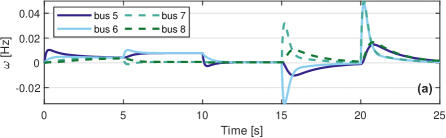
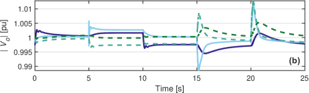
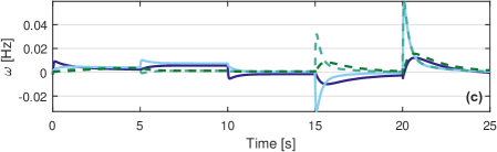
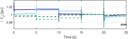
Figure 3: (a)–(b): transient response of the proposed controller in an inductive network under discrete disturbances: from $0.01$ to $10$ s, the conductance and susceptance of the Z load at Bus 9 are reduced by $40\%$ and $50\%$ respectively, the conductance of the Z load at Bus 10 is reduced by $20\%$, and the real power of the CPL at Bus 10 is increased by $40\%$. From $5$ to $15$ s, CB1 is opened. At $20$ s, CB2 to the infinite bus $V_{inf}=0.95\angle 0.6$ pu is closed. (c)–(d): the standard droop control [32] under the same disturbances for comparison

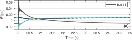
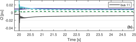
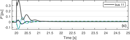
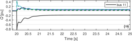
Figure 4: (a)–(b): power sharing of the proposed controller with $20$ ms network time constant when the microgrid is reconnected to a stiff main grid at $20$ s without pre-synchronization. (c)–(d): power sharing of the proposed controller with $1$ ms network time constant under the same disturbance

7 Conclusion

We have presented a stability analysis of the orbit of the microgrid with the proposed control scheme. The analysis has shown that all variables except for the internal frequencies are Lyapunov stable; the internal frequencies are not necessarily Lyapunov stable but do converge to the frequency of the limit cycle. This result makes sense from the observation that frequency by its definition is the derivative of some other state variable. A state variable can remain bounded while its derivative can still vary greatly. Hence the plausible way to prove convergence of the state variables and its derivative is through inspection of the limit sets of the trajectories. Here is where the dissipation plays a role, as a trajectory that continues to dissipate cannot have reached the limit set. Another difficulty we have overcome is that the existence of a limit cycle is often found to be in contradiction with dissipation. The proposed control scheme overcomes this problem by generating the reference voltage only as a result of the speed of the internal reference frame, thus creating an implicit connection between amplitude and frequency.

The practical implications of the proposed control and its stability properties are immense. The smoother voltage transients under step disturbances, as shown in the numerical example, would reduce the chance of overvoltage in smaller-scale microgrids. The global stability guarantee would basically allow AC microgrids to be no less stable than DC microgrids while enjoying other advantages such as more accurate power sharing through the common frequency over the DC microgrid.

Appendix A Proof of the properties of the inner product defined in (27) in Subsection 3.3

We will prove that the inner product defined in (27) satisfies $\langle\mathbf{p},\mathbf{U}\mathbf{q}\rangle=\langle\mathbf{U}^{*}\mathbf{p},\mathbf{q}\rangle$ and $\mathbf{U}>0\Longrightarrow\langle\mathbf{q},\mathbf{U}\mathbf{q}\rangle>0$ for a Hermitian matrix $\mathbf{U}$. First consider a $2$-by-$2$ real matrix $\mathbf{U}=\big{[}a,b;c,d]$ verifying the complex number structure. Let $\mathbf{p}=\big{[}p_{1},p_{2}\big{]}^{\mathsf{T}}$, and $\mathbf{q}=\big{[}q_{1},q_{2}\big{]}^{\mathsf{T}}$. We can write

$$\langle\mathbf{p},\mathbf{U}\mathbf{q}\rangle =\Re\big{\{}\begin{bmatrix}p_{1}^{*}&-jp_{2}^{*}\end{bmatrix}\begin{bmatrix}a&b\\ jc&jd\end{bmatrix}\begin{bmatrix}q_{1}\\ q_{2}\end{bmatrix}\big{\}}$$

$$=\Re\big{\{}ap_{1}^{*}q_{1}+bp_{1}^{*}q_{2}+cp_{2}^{*}q_{1}+dp_{2}^{*}q_{2}\big{\}}.$$

On the other hand,

$$\langle\mathbf{q},\mathbf{U}^{*}\mathbf{p}\rangle =\Re\{\begin{bmatrix}q_{1}^{*}&-jq_{2}^{*}\end{bmatrix}\begin{bmatrix}a^{*}&b^{*}\\ jc^{*}&jd^{*}\end{bmatrix}\begin{bmatrix}p_{1}\\ p_{2}\end{bmatrix}\}$$

$$=\Re\{a^{*}q_{1}^{*}p_{1}+b^{*}q_{1}^{*}p_{2}+c^{*}q_{2}^{*}p_{1}+d^{*}q_{2}^{*}p_{2}\}.$$

Hence $\langle\mathbf{p},\mathbf{U}\mathbf{q}\rangle=\langle\mathbf{U}^{*}\mathbf{p},\mathbf{q}\rangle$. Now assume that $\mathbf{U}$ has a complex number structure, i.e., it has real elements and satisfies $a=d,\,b=-c$. Then we have

$$\langle\mathbf{q},(\mathbf{U}+\mathbf{U}^{*})\mathbf{q}\rangle =\langle\mathbf{q},\mathbf{Q}\mathbf{\Lambda}\mathbf{Q}^{*}\mathbf{q}\rangle$$

$$=\langle\mathbf{Q}^{*}\mathbf{q},\mathbf{\Lambda}\mathbf{Q}^{*}\mathbf{q}\rangle$$

$$=\langle\mathbf{h},\lambda\mathbf{h}\rangle$$

$$=\lambda\Re\{(h_{1}^{*}-jh_{2}^{*})(h_{1}+jh_{2})\}$$

where we used that if $(\mathbf{U}+\mathbf{U}^{*})$ has a complex number structure, its eigenvalue matrix is given by $\mathbf{\Lambda}=\lambda\mathbf{I}$. Hence $\mathbf{U}+\mathbf{U}^{*}>0\Longrightarrow\langle\mathbf{q},\mathbf{U}\mathbf{q}\rangle>0$. The same holds if $\mathbf{U}$ has a block dimension greater than $1$.

References

• [1] Olaoluwapo Ajala, Minghui Lu, Brian Johnson, Sairaj V Dhople, and Alejandro Domínguez-García. Model reduction for inverters with current limiting and dispatchable virtual oscillator control. IEEE Transactions on Energy Conversion, 37(4):2250–2259, 2021.
• [2] Marian Anghel, Federico Milano, and Antonis Papachristodoulou. Algorithmic construction of Lyapunov functions for power system stability analysis. IEEE Transactions on Circuits and Systems I: Regular Papers, 60(9):2533–2546, 2013.
• [3] Nazmi Burak Budanur, Daniel Borrero-Echeverry, and Predrag Cvitanović. Periodic orbit analysis of a system with continuous symmetry—a tutorial. Chaos: An Interdisciplinary Journal of Nonlinear Science, 25(7), 2015.
• [4] Francesco Bullo and Andrew D. Lewis. Geometric Control of Mechanical Systems, volume 49 of Texts in Applied Mathematics. Springer Verlag, New York-Heidelberg-Berlin, 2004.
• [5] Sina Yamac Caliskan and Paulo Tabuada. Compositional transient stability analysis of multimachine power networks. IEEE Transactions on Control of Network systems, 1(1):4–14, 2014.
• [6] Sina Yamac Caliskan and Paulo Tabuada. Correction to “compositional transient stability analysis of multimachine power networks”. IEEE Transactions on Control of Network Systems, 4(3):676–677, 2016.
• [7] H.-D. Chiang and M.E. Baran. On the existence and uniqueness of load flow solution for radial distribution power networks. IEEE Transactions on Circuits and Systems, 37(3):410–416, 1990.
• [8] Hsiao-Dong Chiang. Direct methods for stability analysis of electric power systems: theoretical foundation, BCU methodologies, and applications. John Wiley & Sons, 2011.
• [9] Marcello Colombino, Dominic Groß, Jean-Sébastien Brouillon, and Florian Dörfler. Global phase and magnitude synchronization of coupled oscillators with application to the control of grid-forming power inverters. IEEE Transactions on Automatic Control, 64(11):4496–4511, 2019.
• [10] Stephan De Bievre, François Genoud, and Simona Rota Nodari. Orbital stability: analysis meets geometry. Nonlinear Optical and Atomic Systems: At the Interface of Physics and Mathematics, pages 147–273, 2015.
• [11] Claudio De Persis and Nima Monshizadeh. Bregman storage functions for microgrid control. IEEE Transactions on Automatic Control, 63(1):53–68, 2017.
• [12] Huagui Duan, Yiming Long, and Chaofeng Zhu. Index iteration theories for periodic orbits: old and new. Nonlinear Analysis, 201:111999, 2020.
• [13] Ivar Ekeland. Convexity methods in Hamiltonian mechanics, volume 19. Springer Science & Business Media, 2012.
• [14] S Fiaz, Daniele Zonetti, Roméo Ortega, Jacquelien MA Scherpen, and AJ van der Schaft. On port-Hamiltonian modeling of the synchronous generator and ultimate boundedness of its solutions. IFAC Proceedings Volumes, 45(19):30–35, 2012.
• [15] Shaik Fiaz, Daniele Zonetti, Romeo Ortega, Jacquelien MA Scherpen, and AJ Van der Schaft. A port-Hamiltonian approach to power network modeling and analysis. European Journal of Control, 19(6):477–485, 2013.
• [16] Nikos Hatziargyriou, Jovica Milanovic, Claudia Rahmann, Venkataramana Ajjarapu, Claudio Canizares, Istvan Erlich, David Hill, Ian Hiskens, Innocent Kamwa, Bikash Pal, et al. Definition and classification of power system stability–revisited & extended. IEEE Transactions on Power Systems, 36(4):3271–3281, 2020.
• [17] John Hauser and Chung Choo Chung. Converse Lyapunov functions for exponentially stable periodic orbits. Systems & Control Letters, 23(1):27–34, 1994.
• [18] Xiuqiang He, Verena Häberle, Irina Subotić, and Florian Dörfler. Nonlinear stability of complex droop control in converter-based power systems. IEEE Control Systems Letters, 7:1327–1332, 2023.
• [19] Jorgen K Johnsen, Florian Dorfler, and Frank Allgower. L2-gain of port-Hamiltonian systems and application to a biochemical fermenter model. In 2008 American Control Conference, pages 153–158. IEEE, 2008.
• [20] Taouba Jouini and Zhiyong Sun. Frequency synchronization of a high-order multiconverter system. IEEE Transactions on Control of Network Systems, 9(2):1006–1016, 2021.
• [21] Mahmoud Kabalan, Pritpal Singh, and Dagmar Niebur. Nonlinear Lyapunov stability analysis of seven models of a dc/ac droop controlled inverter connected to an infinite bus. IEEE Transactions on Smart Grid, 10(1):772–781, 2017.
• [22] Hassan K Khalil. Nonlinear Systems; 3rd ed. Prentice-Hall, Upper Saddle River, NJ, 2002.
• [23] James L Kirtley. Electric power principles: sources, conversion, distribution and use. John Wiley & Sons, 2010.
• [24] Ramachandra Rao Kolluri, Iven Mareels, Tansu Alpcan, Marcus Brazil, Julian de Hoog, and Doreen Anne Thomas. Stability and active power sharing in droop controlled inverter interfaced microgrids: Effect of clock mismatches. Automatica, 93:469–475, 2018.
• [25] Ian R Manchester and Jean-Jacques E Slotine. Transverse contraction criteria for existence, stability, and robustness of a limit cycle. Systems & Control Letters, 63:32–38, 2014.
• [26] Nima Monshizadeh, Pooya Monshizadeh, Romeo Ortega, and Arjan van der Schaft. Conditions on shifted passivity of port-Hamiltonian systems. Systems & Control Letters, 123:55–61, 2019.
• [27] Peter J Olver. Applications of Lie groups to differential equations, volume 107. Springer Science & Business Media, 1993.
• [28] Romeo Ortega, Nima Monshizadeh, Pooya Monshizadeh, Dmitry Bazylev, and Anton Pyrkin. Permanent magnet synchronous motors are globally asymptotically stabilizable with PI current control. Automatica, 98:296–301, 2018.
• [29] SangWoo Park, Richard Y Zhang, Javad Lavaei, and Ross Baldick. Uniqueness of power flow solutions using monotonicity and network topology. IEEE Transactions on Control of Network Systems, 8(1):319–330, 2020.
• [30] Lawrence Perko. Differential Equations and Dynamical Systems, volume 7. Springer Science & Business Media, 2013.
• [31] Kaare Brandt Petersen, Michael Syskind Pedersen, et al. The matrix cookbook. Technical University of Denmark, 7(15):510, 2008.
• [32] Nagaraju Pogaku, Milan Prodanovic, and Timothy C Green. Modeling, analysis and testing of autonomous operation of an inverter-based microgrid. IEEE Transactions on Power Electronics, 22(2):613–625, 2007.
• [33] Reinhold Remmert. Theory of complex functions, volume 122. Springer Science & Business Media, 1991.
• [34] Stefano Riverso, Fabio Sarzo, and Giancarlo Ferrari-Trecate. Plug-and-play voltage and frequency control of islanded microgrids with meshed topology. IEEE Transactions on Smart Grid, 6(3):1176–1184, 2014.
• [35] Clarence W Rowley, Ioannis G Kevrekidis, Jerrold E Marsden, and Kurt Lust. Reduction and reconstruction for self-similar dynamical systems. Nonlinearity, 16(4):1257, 2003.
• [36] Giovanni Russo and Jean-Jacques E Slotine. Symmetries, stability, and control in nonlinear systems and networks. Physical Review E, 84(4):041929, 2011.
• [37] Ernest K Ryu and Stephen Boyd. Primer on monotone operator methods. Appl. comput. math, 15(1):3–43, 2016.
• [38] Johannes Schiffer, Denis Efimov, and Romeo Ortega. Global synchronization analysis of droop-controlled microgrids—a multivariable cell structure approach. Automatica, 109:108550, 2019.
• [39] Johannes Schiffer, Romeo Ortega, Alessandro Astolfi, Jörg Raisch, and Tevfik Sezi. Conditions for stability of droop-controlled inverter-based microgrids. Automatica, 50(10):2457–2469, 2014.
• [40] John W Simpson-Porco. Equilibrium-independent dissipativity with quadratic supply rates. IEEE Transactions on Automatic Control, 64(4):1440–1455, 2018.
• [41] Chrysovalantis Spanias and Ioannis Lestas. A system reference frame approach for stability analysis and control of power grids. IEEE Transactions on Power Systems, 34(2):1105–1115, 2018.
• [42] Felix Strehle, Pulkit Nahata, Albertus Johannes Malan, Sören Hohmann, and Giancarlo Ferrari-Trecate. A unified passivity-based framework for control of modular islanded ac microgrids. IEEE Transactions on Control Systems Technology, 30(5):1960–1976, 2021.
• [43] Irina Subotić, Dominic Groß, Marcello Colombino, and Florian Dörfler. A Lyapunov framework for nested dynamical systems on multiple time scales with application to converter-based power systems. IEEE Transactions on Automatic Control, 66(12):5909–5924, 2020.
• [44] Russ Tedrake. Underactuated Robotics. Course Notes for MIT 6.832, 2023.
• [45] Michele Tucci and Giancarlo Ferrari-Trecate. A scalable, line-independent control design algorithm for voltage and frequency stabilization in ac islanded microgrids. Automatica, 111:108577, 2020.
• [46] Arjan Van der Schaft. L2-gain and passivity techniques in nonlinear control. Springer, 2000.
• [47] Arjan Van der Schaft. Characterization and partial synthesis of the behavior of resistive circuits at their terminals. Systems & Control Letters, 59(7):423–428, 2010.
• [48] Vijay Vittal and James D McCalley. Power System Control and Stability. Wiley, Hoboken, NJ, USA, 3 edition, 2019.
• [49] Xiongfei Wang, Yun Wei Li, Frede Blaabjerg, and Poh Chiang Loh. Virtual-impedance-based control for voltage-source and current-source converters. IEEE Transactions on Power Electronics, 30(12):7019–7037, 2014.
• [50] Bowen Yi, Romeo Ortega, Dongjun Wu, and Weidong Zhang. Orbital stabilization of nonlinear systems via mexican sombrero energy shaping and pumping-and-damping injection. Automatica, 112:108661, 2020.