Distance-Preserving Generative Modeling of Spatial Transcriptomics

Abstract.

Spatial transcriptomics data is invaluable for understanding the spatial organization of gene expression in tissues. There have been consistent efforts in studying how to effectively utilize the associated spatial information for refining gene expression modeling. We introduce a class of distance-preserving generative models for spatial transcriptomics, which utilizes the provided spatial information to regularize the learned representation space of gene expressions to have a similar pair-wise distance structure. This helps the latent space to capture meaningful encodings of genes in spatial proximity. We carry out theoretical analysis over a tractable loss function for this purpose and formalize the overall learning objective as a regularized evidence lower bound. Our framework grants compatibility with any variational-inference-based generative models for gene expression modeling. Empirically, we validate our proposed method on the mouse brain tissues Visium dataset and observe improved performance with variational autoencoders and scVI (Lopez et al., 2018) used as backbone models.

1. Introduction

Spatial transcriptomic (ST) technologies enable the measurement of expression levels of multiple genes systematically throughout tissue space, deepening the understanding of cellular organizations and interactions within tissues as well as illuminating biological insights in neuroscience, developmental biology, and a range of diseases, including cancer (Yu et al., 2022). An example of the ST technologies is Visium by 10x Genomics, which enables the capture of whole transcriptomes from tissue slices. However, Visium typically does not have single-cell resolution (Chen et al., 2023). This is also the case with many other existing ST technologies, such as NanoString GeoMx (Dries et al., 2021a). Therefore, it is necessary to develop further approaches when inaccessibility to precise localization of gene expression at the single-cell level becomes a critical bottleneck in the analyzing process. Meanwhile, the data generated is inevitably noisy, potentially complicating the interpretation of spatial gene expression patterns.

Generative modeling provides a solution to these problems by capturing precise representations from spatial transcriptomic data with powerful deep neural networks. The process of learning representations is to extract higher-level latent variables that significantly reduce the data dimension while retaining as much information as possible. The latent variables can be used for downstream analysis, such as clustering or visualization to identify the cell types or subtypes, batch correction, visualization, clustering, and differential expression (Lopez et al., 2018; Du et al., 2020). In the meantime, existing works have depicted a positive correlation between gene expression and their relative spatial locations (Hu et al., 2021; Sun et al., 2020). It remains an open question whether, in practice, we can integrate this idea into other powerful deep generative learning frameworks to improve modeling power.

In this paper, building upon various variational inference models, we develop a novel generative learning method to extract coherent spatial-informative representation from data. Our novelty lies in leveraging the cell-by-coordinate information to directly modify the learned latent representations. Specifically, the idea is to enforce their probabilistic encoders to produce samples that preserve the pair-wise distance measure of the provided original spatial information. While similar notions of representation learning have appeared in existing machine learning literature, none has yet established a formal definition for the distant-preserving property. In our work, we provide a theoretical definition of distance-preserving generative models. Furthermore, we establish a formal connection between the distortion loss and our definition of the distance-preserving generative models, showing that the upper distortion level is directly proportional to the distortion loss. This allows us to treat the distance-preserving generative learning problem as a constrained optimization problem, with the original loss of the generative model as the objective function, and the distortion loss as the constraint. We further propose to relax this constrained optimization problem into a regularized optimization problem, such that the distortion loss can be easily implemented as a wrapper to existing variational-inference-based generative models. Lastly, our proposed method is applied to real-world datasets such as the Visium dataset of fresh frozen mouse brain tissue (Strain C57BL/6) with 10x Genomics obtained from BioIVT Asterand. See Figure 1 for an illustration of the dataset. We adopt Moran’s I and Geary’s C statistics (Li et al., 2007) in our evaluation, which reflects the spatial autocorrelation between the latent representation and the gene locations. The experiment results support that the methods that we have developed can enhance the resolution and quality of spatial transcriptomic data, facilitating more accurate mapping of gene expression patterns at a near-single-cell level, reflected by the decreased reconstruction error of the input testing Visium data.

Contributions

This paper makes several key contributions to the field of spatial transcriptomics analysis and understanding how to incorporate spatial information in gene expression modeling:

1. We provide a rigorous and systematic formal definition of distance-preserving generative models, which, to our knowledge, has not yet been established in existing literature.

2. We derive the distortion loss as an upper bound to the distortion constant. This, to some extent, establishes theoretical guarantees that the distortion loss is a valid loss function for the purpose of enforcing the distance-preserving property.

3. In practice, as our method is directly inspired by single-cell spatial transcriptomics, we tailor the method to be more user-friendly by suggesting the regularized optimization, which also makes it directly compatible with existing variational-inference-based deep generative modeling approaches, and can be easily applied to real-world biological data analysis.

Figure 1. The 2D representations of cells of Mouse Brain Serial Datasets anterior 1 using UMAP(McInnes et al., 2018) and their spatial locations, colored by clustering results on the UMAP coordinates. The usual workflow first performs dimension reduction, ignoring the spatial information, and then analyzes the gene expression patterns on the spatial domain.

2. Related Works

This section summarizes some major works related to methodology and application. We defer some additional related works in Appendix C.

Geometry-grounded machine learning

Geometry-grounded machine learning is a recently emerging topic. Compared to traditional machine learning, aside from considering only the direct relationship between the input and output, these models also consider the data’s geometric structure as part of the learning objective. In particular, distance-preserving is a relatively weaker notion compared to, for example, isometry (Yonghyeon et al., 2021; Lee et al., 2021; Beshkov et al., 2022), which is mainly discussed in our work. (Benaim and Wolf, 2017) introduced distance-preserving mappings in the field of unsupervised domain mapping using GANs. (Port et al., 2020; Kim et al., 2020) show that enforcing the distance-preserving property is a convincing way to learn meaningful mappings from face images to audio domains, highlighting the real-world application potentials. (Chen et al., 2022) enforced distance preserving in learning VAEs by formulating it as the objective of a constraint optimization problem. We also note that distance-preserving is also highly similar to the invariance constraint (Hadsell et al., 2006; Mao et al., 2019) that has been introduced in adversarial learning.

Prior works that use similar designs of distance-preserving loss have largely confined it to a heuristical act without providing further justifications or insights. In our paper, bridging the mathematical definition of the bi-Lipschitz condition, we formally define the notion of locality for generative models. We theoretically show how minimizing the previously proposed loss helps minimize distortion.

Machine Learning in Spatial Transcriptomics

Spatial transcriptomics data modeling has been of broad interest to scholars in the field of machine learning. In particular, we focus on statistical machine learning methods designed for such task (Zeng et al., 2022). To capture spatial correlation exhibited from the data, statistical models such as marked point process (Edsgärd et al., 2018), Gaussian process (Svensson et al., 2018) and generalized linear spatial models (Sun et al., 2020; Zhu et al., 2021). A common theme of these methods is that they all rely on constructing some notion of covariance matrix over the spatial locations with cubic computational complexity, which could be computationally inefficient. Notably, the seminal work of scVI (Lopez et al., 2018) stands closest to our work. They also use variational inference to model data representations and extend to a broad spectrum of downstream analysis such as missing genes imputation (Lopez et al., 2019). However, their work does not naturally extend to account for spatial information present in the data explicitly. Recently, deep learning models such as SpaCGN (Hu et al., 2021) and GLISS (Zhu and Sabatti, 2020) are graph-based methods that have been proposed to aggregate spatial information into data modeling directly.

Our work differs from existing works in that it provides a general variational representation learning perspective towards modeling spatial transcriptomics data, where the spatial information is incorporated into the model via a learned isometric mapping. This makes our method both concise and flexible compared to other existing methods.

3. Background

In this section, we provide a brief review of the relevant variational inference framework.

VAE and CVAE

Variational autoencoder (VAE) (Bengio and LeCun, 2014) is a popular type of generative model. Given data drawn from the data distribution $p(y)$, the goal of a VAE is to learn a latent variable model that approximates the true data distribution by:

(1) $$\addcontentsline{lla}{section}{\numberline{\string\crtrefnumber{eq:lvm}}{e}q:lvm}p_{\phi}(y)=\int p_{\phi}(y|z)p(z)dz,$$

where $z$ is the latent variable, $p_{\theta}(y|z)$ is the parameterized likelihood function of $y$ given $z$, and $p(z)$ is the prior dsitribution over $z$ specified a priori. Training the model specified in (1) is done by maximizing the evidence lower bound (ELBO) of its likelihood function:

$$\log p_{\phi}(y) \geq\mathbb{E}_{z\sim q_{\theta}(z|y)}\log p_{\phi}(y|z)-D_{\rm KL}\left(q_{\theta}(z|y)\|p(z)\right).$$

The derivation can be found in Appendix D. The loss of a VAE is defined as the negative of the ELBO, and it can be estimated by:

(2) $$\addcontentsline{lla}{section}{\numberline{\string\crtrefnumber{eq:vae-loss}}{e}q:vae-loss}\ell_{\mathrm{VAE}}=\sum_{i=1}^{N}-\log p_{\phi}(y_{i}|z_{i})+D_{\rm KL}\left(q_{\theta}(z_{i}|y_{i})\|p(z_{i})\right).$$

The model parameter $\theta$ is learned by minimizing the loss function in (2).

The posterior $q_{\theta}$ and likelihood $p_{\phi}$ can also be viewed as random functions. Therefore, the learning outcome of a VAE can be more compactly written as a probabilistic encoder and decoder pair defined as:

$$f_{\theta}:\mathcal{Y}\to\mathcal{Z},$$

$$g_{\phi}:\mathcal{Z}\to\mathcal{Y},$$

A conditional variational encoder (CVAE) (Sohn et al., 2015; Wu et al., 2023) is an extension of VAE, where it consists of a set of encoder and decoder pairs where their domains also include an additional space of context information, written as:

$$f_{\theta}:\mathcal{Y}\times\mathcal{C}\to\mathcal{Z},$$

$$g_{\phi}:\mathcal{Z}\times\mathcal{C}\to\mathcal{Y}.$$

Other than that, the training procedure is basically identical to VAE.

scVI (single-cell Variational Inference)

scVI (Lopez et al., 2018) is a leading deep generative model for analyzing single-cell RNA sequencing (scRNA-seq) data. It employs a CVAE architecture to model gene expression patterns across individual cells. In scVI, the input consists of gene expression counts for each cell, while the model aims to learn a latent representation that captures biological variability. The model accounts for technical factors such as library size and batch effects, which are treated as observed variables. Specifically, scVI uses the normalized gene expression counts as the target variable, with the library size included as a nuisance variable to be inferred. Batch information, when available, is incorporated as conditional information to help disentangle technical from biological variability. This approach allows scVI to perform various downstream tasks, including normalization, batch correction, imputation, and dimensionality reduction, making it a versatile tool for single-cell transcriptomics analysis.

4. Distance-preserving generative models

In this section, we will introduce a new class of distance-preserving generative models for spatial transcriptomics modeling analysis. The section is organized as follows: We first provide the problem formulation, then we define the distortion constant of generative models (Definition 4.1). Then, we propose a decomposable loss function named distortion loss and prove that it upper bounds the distortion constant. Next, we propose a masking procedure that provides flexibility in modifying the span of the neighborhood considered in the distortion loss. Finally, we briefly summarize the entire model architecture.

4.1. Problem formulation

Let $y\in\mathcal{Y}$ denote the target attributes (gene expressions) that we aim to model with generative models. Let $s\in\mathcal{S}$ denote the spatial information. We are given a set of spatial transcriptomic data of size $N$:

$$\mathcal{D}=\left\{y_{i},s_{i}\right\}_{i=1}^{N},$$

where each entry corresponds to a cell. Our goal is to learn a generative model from the data that extracts the latent representation of the data. Specifically, we require that the generative model consist of a probabilistic encoder-decoder pair of parameterized random functions. Without loss of generality, we assume that they take the following form:

$$f_{\theta}:\mathcal{Y}\to\mathcal{Z},$$

$$g_{\phi}:\mathcal{Z}\to\mathcal{Y},$$

where we denote $z\in\mathcal{Z}$ as the latent variable. To facilitate theoretical analysis, we assume that the data in $\mathcal{D}$ is drawn i.i.d. from some joint distribution over $\mathcal{Y}\times\mathcal{Z}$. We hope to efficiently utilize the spatial information $s_{i}$ that is present in the dataset to refine our learned gene expression. An illustration of the structure of the dataset is provided in Figure 2.

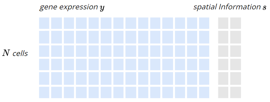
Figure 2. Illustration of the paired dataset $\mathcal{D}$. Each row corresponds to a different cell ($N$ cells in total). The columns on the left (blue squares) represent gene expression data ($y$) for each cell, while the columns on the right (gray squares) represent spatial information ($s$) associated with each cell.

4.2. Distance-preserving and distortion

To illustrate why distance-preserving is a helpful concept to consider in generative modeling for spatial transcriptomics modeling, let’s consider the following example. Cells that are physically close to one another often originate from similar tissue types. Consequently, these neighboring cells are likely to exhibit homogeneity in various attributes of interest, such as biological functions and patterns of highly variable gene expression. When applying representation-based generative models to analyze such data, the goal is to learn latent representations that serve as informative, high-level abstractions of the underlying biological complexity. In spatial transcriptomics, spatial information is inherently valuable and provides crucial context for understanding cellular behavior and tissue organization. A well-designed generative model should effectively incorporate this spatial information to learn more accurate and biologically meaningful representations. By doing so, the model can capture not only the gene expression profiles of individual cells but also the spatial relationships and tissue-level patterns that are essential for a comprehensive understanding of cellular function and organization. This example underscores the potential of integrating spatial data with gene expression information to enhance our ability to uncover biological insights and generate more robust, context-aware models of cellular systems.

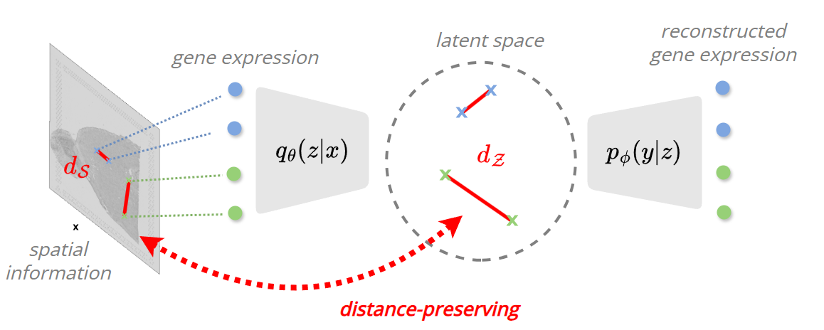
Figure 3. Model architecture with vanilla VAE as its backbone. In the latent space, the distortion loss ($\ell_{\textrm{DIS}}$) enforces distance preservation between the spatial domain ($s$) and the latent space ($z$). The masking procedure encourages the distance-preserving property locally, focusing on neighboring cells rather than all cell pairs.

To incorporate spatial information into learning a generative model, a useful practice is to directly enforce the distance measure of the latent representation space to be similar to the space where spatial information is drawn. In the domain of studying deterministic embedding functions, the distortion measure (Chennuru Vankadara and von Luxburg, 2018) is usually used to characterize this property. Formally, let $d_{\mathcal{X}}$ and $d_{\mathcal{Y}}$ denote the distance metric defined in space $\mathcal{X}$ and $\mathcal{Y}$. An embedding function $f:\mathcal{X}\to\mathcal{Y}$ is an embedding of distortion $L$, if there exists some $\lambda>0$, such that for all $x,x^{\prime}\in\mathcal{X}$, the following condition hold:

(3) $$\lambda d_{\mathcal{X}}(x,x^{\prime})\leq d_{\mathcal{Y}}\left(y^{\prime},y^{\prime}\right)\leq L\cdot\lambda d_{\mathcal{X}}(x,x^{\prime}),$$

where $y=f(x),y^{\prime}=f(x^{\prime})$. Distortion is also known as the bi-Lipshitz condition (Mahabadi et al., 2018; Verine et al., 2023). $L$ is also called the worst case distortion (Chennuru Vankadara and von Luxburg, 2018). Verbally, this property states that the outputs of the embedding function have pairwise distances that are equal to the pairwise distances of its inputs up to some scaling parameter $L$. Therefore, we collectively refer to the functions that exhibit this property as distance-preserving functions.

While the notion of distance-preserving functions has been proposed, there has not yet been a rigorous mathematical definition that generalizes to generative models. This generalization is non-trivial in the sense that (1) the posterior network is a probabilistic function, which means that, unlike deterministic functions, its output can only be accessed via sampling, and (2) If the posterior distribution is supported on an infinite space, then the above definition would be uninformative. For example, in the worst case scenario, we can always sample $y_{1},y_{2}$ from the posterior function such that does not hold true, and (3) The generative model’s output can be distance-preserving with respect to any other contextual information, not only just the inputs. For example, in spatial transcripts modeling, the spatial information is the contextual information that should be modeled for distance-preserving, not the input of gene expression itself.

Based on these analyses, we formally extend the definition of distance-preserving generative models, summarized as follows:

Definition 4.1 (Distance-preserving generative models).

Denote the observation data tuple $x:=(y,s)$, where $s$ is the spatial information of $y$. Denote $\mathcal{Z}$ as the latent space. For a generative model with a probabilistic encoder:

$$f:\mathcal{Y}\to\mathcal{Z},$$

if there exist some $\lambda>0$, such that the following condition holds:

(4) $$\addcontentsline{lla}{section}{\numberline{\string\crtrefnumber{eq:def}}{e}q:def}\mathbb{P}\left(\lambda d_{\mathcal{S}}(s,s^{\prime})\leq d_{\mathcal{Z}}\left(z,z^{\prime}\right)\leq L\cdot\lambda d_{\mathcal{S}}(s,s^{\prime})\right)\geq 1-\varepsilon,$$

where the probability is taken with respect to the randomness of the following generation process:

(5) $$\addcontentsline{lla}{section}{\numberline{\string\crtrefnumber{eq:gen-process}}{e}q:gen-process}x,x^{\prime}\overset{iid}{\sim}p(x),\ z\sim f_{\theta}(y),\ z^{\prime}\sim f_{\theta}(y^{\prime}),$$

then we say that the generative model is a distance-preserving generative model.

We call the smallest $L$ that satisfies (4) as the distortion constant, where we omit its dependency on $\varepsilon$ when clear from the context. Intuitively, $L$ measures the dispersion of the probabilistic decoder. If $L$ is small, then the probabilistic encoder has a high probability of generating samples such that the distance structure of the provided spatial information input is preserved in its outputs. In the context of spatial transcriptomic, this corresponds to the extracted latent gene expression to lie in a low-dimensional geometric space that has a similar structure as their original spatial location.

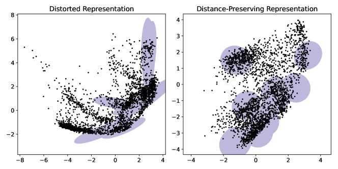
Figure 4. Visualization of latent representation space obtained from scVI (left) and scVI regularized with distortion loss (right). More isotropic and homogeneous ellipses indicate more distance-preserving.

4.3. Tractable learning

In this part, we wish to further derive a tractable learning objective that can enforce the outlined properties in this Definition 4.1. Specifically, define $\lambda$ as in (4), we show that there exists a simple, decomposable loss function that can do so:

(6) $$\addcontentsline{lla}{section}{\numberline{\string\crtrefnumber{eq:iso-pop}}{e}q:iso-pop}\mathcal{L}_{\mathrm{DIS}}=\mathbb{E}[\left|d_{\mathcal{Z}}(z,z^{\prime})-\lambda\cdot d_{\mathcal{S}}(s,s^{\prime})\right|],$$

where the expectation is taken with respect to the generation process outlined in (5). We call (6) the distortion loss.

Mathematically, we show that (6) can provably translate into the upper bound of the distortion constant $L$ defined in Definition 4.1. Before we present this main result, we first define some necessary notations in Lemma 4.2:

Lemma 4.2.

For any given distribution defined on some space $\mathcal{X}\subseteq\mathbb{R}^{n}$, given arbitrary $0<\delta<1$, there exist some $0<M_{1}<M_{2}<+\infty$, such that:

(7) $$\mathbb{P}\left(M_{1}\leq\left|d_{\mathcal{X}}(x,x^{\prime})\right|\leq M_{2}\right)\geq 1-\delta,$$

where $x,x^{\prime}$ are drawn i.i.d. from this distribution.

The proof of Lemma 4.2 is deferred to Appendix A. Lemma 4.2 can be applied to the spatial information variable $s,s^{\prime}$, which we assume are drawn i.i.d. according to the generative process (5). This is used in proving the following main Theorem of this paper:

Theorem 4.3.

Let $\delta,M_{1},M_{2}$ be given from Lemma 4.2 applied to the distribution of spatial information $s$. Let $\mathcal{L}_{DSI}$ be the distortion loss defined in (6). Then the generative model defined in 4.1 has distortion constant:

(8) $$\addcontentsline{lla}{section}{\numberline{\string\crtrefnumber{eq:prop-L}}{e}q:prop-L}L\leq\frac{M_{2}}{M_{1}}+\frac{\mathcal{L}_{\mathrm{DIS}}}{\lambda M_{1}\varepsilon(1-\delta)}.$$

Theorem 4.3 states that the upper bound of the distortion constant of the generative model scales positively with the distortion loss. Therefore, this means that we can expect that minimizing $\mathcal{L}_{DIS}$ will enforce the probabilistic encoder of the generative model to have a high probability of generating samples that have similar distance structure as the spatial information.

As a decomposable loss function, the distortion loss (6) can be estimated in an unbiased fashion using Monte Carlo. Given dataset:

$$(y_{i},s_{i})\overset{iid}{\sim}p(y,s),\ i=\left\{1,\ldots,N\right\},$$

denote the latent representations mapped from each $y_{i}$ as $z_{i}$, we can simply compute the empirical distortion loss as follows:

(9) $$\addcontentsline{lla}{section}{\numberline{\string\crtrefnumber{eq:loss-mc}}{e}q:loss-mc}\ell_{DIS}=\frac{1}{N^{2}}\sum_{i\neq j}|d_{\mathcal{Z}}(z_{i},z_{j})-\lambda\cdot d_{\mathcal{S}}(s_{i},s_{j})|.$$

As $\lambda$ is not known, we set the variable $\lambda$ as a learnable parameter. (9) can then be minimized using gradient descent algorithms.

We further comment on some practical aspects of implementing the loss (6). While we have illustrated that neighboring cells are homogeneous across patterns that may be informative for learning latent representations, it is usually not the case that such patterns are shared across cells of longer spatial distances. Intuitively, it may be helpful to ”mask” the cells that lie too far apart from each other and only keep the isometry property to hold at a local scale for better learning outcomes.

To encourage learning over just local scales, denote the pairwise distance matrix of the latent space and the spatial coordinates:

$$D_{z}=[d_{\mathcal{Z}}(z_{i},z_{j})]_{ij}^{N},\quad D_{s}=[d_{\mathcal{S}}(s_{i},s_{j})]_{ij}^{N},$$

Let $V_{\mathcal{D}}$ denote a prespecified set of edges between pairs of spatial coordinates $(s_{i},s_{j})$ contained in the dataset $\mathcal{D}$. Denote the index matrix:

$$G(s_{i},s_{j}):=\left\{\begin{array}[]{rl}1&{\rm if}~{}(s_{i},s_{j})\in V,\\ 0&{\rm otherwise.}\end{array}\right.$$

using We define the empirical masked isometric loss as:

(10) $$\addcontentsline{lla}{section}{\numberline{\string\crtrefnumber{eq:masked-loss}}{e}q:masked-loss}\overline{\ell}_{\rm DIS}=\frac{1}{N^{2}}\left\|G\odot D_{z}-\lambda\cdot G\odot D_{s}\right\|_{1},$$

where $\|\cdot\|_{1}$ denotes the entry-wise $\ell_{1}$ norm of matrices, and $\odot$ denotes the Hadamard product. The choice of $V$ can be specified with different methods. We recommend the use of classification or clustering algorithms based on the spatial coordinate matrix, such as K-nearest neighbors and K-Means, as long as the $V$ reflects a reasonable neighborhood of cells. It is also hypothetically effective to adopt clustering algorithms designed specifically for spatial transcriptomic analysis such as SpaGCN (Hu et al., 2021) for constructing $V$.

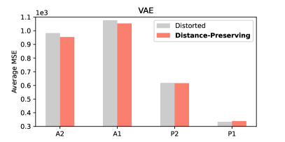
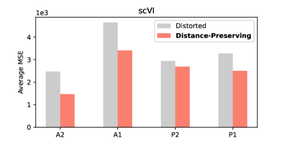
Figure 5. Mean squared error (MSE) of scVi and VAE on 4 test datasets, with and without distance-preserving penalty, averaged over 5 repeated trials. Enforcing distance-preserving property induces smaller reconstruction errors of log-normalized and library-size-adjusted data.

4.4. General model

We aim to learn a generative model of the spatial transcriptomic data that preserves the distance metric in its latent representation space. This is illustrated in Figure 3, and can be formulated as the following constrained optimization problem:

$$\begin{array}[]{ll}\displaystyle\min_{\theta,\phi,\lambda}&\ell_{\mathrm{VAE}}\\ \textrm{s.t.}&\overline{\ell}_{\mathrm{DIS}}\leq c_{1},\lambda>0,\end{array}$$

where $\ell_{\mathrm{VAE}}$ is the loss function of the backbone VAE model. $\overline{\ell}_{\mathrm{ISO}}$ is defined in (10), $c_{1}$ is some arbitrary constant. There are no explicit modeling restrictions of the backbone VAE model to choose from. The constrained optimization problem above is expensive to solve, and we instead propose to relax it into a regularized version:

(11) $$\addcontentsline{lla}{section}{\numberline{\string\crtrefnumber{eq:l}}{e}q:l}\min_{\theta,\phi,\lambda}\ell:=\ell_{\mathrm{VAE}}+\alpha\overline{\ell}_{\mathrm{DIS}},$$

where $\alpha>0$ is the regularization coefficient. The regularized objective function in 11 is easy to implement, and only requires the distortion loss to be implemented as a wrapper function to the original VAE loss. An illustration of the model architecture is illustrated in Figure 3.

5. Experiments

In this section, we conduct experiments on spatial transcriptomic data to validate our proposal. In this section, we first describe our basic experimental setups. Second, we show the main experiment results under our evaluation criterion. Third, we comment on the properties of our proposed method by showing the results of our sensitivity analysis.

Table 1. Moran’s I and Geary’s C of the latent representation extracted by scVi and VAE on 4 test datasets, with and without distance-preserving penalty, averaged over 5 repeated trials. Enforcing distance-preserving property induces stronger spatial autocorrelations.

	Method	Moran’s I				Geary’s C
		A2	A1	P2	P1	A2	A1	P2	P1
Distorted	VAE	0.62(0.07)	0.55(0.05)	0.52(0.05)	0.52(0.03)	0.36(0.06)	0.41(0.03)	0.49(0.05)	0.43(0.03)
	scVI	0.43(0.03)	0.52(0.04)	0.37(0.02)	0.45(0.04)	0.57(0.03)	0.48(0.04)	0.62(0.02)	0.55(0.04)
Distance Preserving	VAE	0.64(0.02)	0.60(0.03)	0.56(0.06)	0.49(0.06)	0.35(0.02)	0.37(0.02)	0.45(0.07)	0.46(0.05)
	scVI	0.45(0.04)	0.52(0.04)	0.43(0.02)	0.47(0.03)	0.55(0.05)	0.48(0.04)	0.57(0.02)	0.53(0.03)

5.1. Experiment setups

Table 2. 10X Genomics Visium Sagittal mouse brain datasets summary.

Dataset	#genes	#spots
P1	31053	3353
P2	31053	3293
A1	31053	2696
A2	31053	2825

Data

We acquire 4 publically available Mouse Brain Serial Datasets, including anterior (A) and posterior (P), section 1 and 2. The data are preprocessed using Seurat v5 (Hao et al., 2023) according to their tutorial. The resulting data contain $\sim 3000$ spatial spots and $p=31053$ genes. We only select $3000$ highly variable genes to ensure model stability.

To construct training and test datasets, we use the gene expression in the same region but from different sections as training and test data (e.g. P1 as a training set and P2 as a test set). The logic behind this is that we hypothesize that gene expressions from the same region are highly correlated and should exhibit minor distribution shifts. Thus, we get four pairs of training-test datasets. For brevity, we refer to them by the name of the test dataset.

Model description

We test out our method using both VAE and scVI as backbones. The VAE is set up with one layer of dimension of $64$ for both the encoder and decoder, and the latent space dimension is set to $4$. The data is preprocessed by log-normalizing, adjusting for the library size of the data, and extracting $256$ principal components from the raw data. The likelihood and prior of the VAE are all set to be Gaussian. We set the weight of the KL term in the loss function of VAE to $10^{-2}$ (See Appendix F). The training process is terminated if no improvement of over $10^{-2}$ has been observed over $10$ epochs. The regularization coefficient is set to $50$. For scVI, we adopt implementation from the developed Python package. The model is set with one hidden layer of $128$ dimension. The latent space is set to be of dimension $10$. We do not transform the data here and we use the negative binomial distribution to model the gene likelihood. The training process is terminated after no improvement of over $30$ has been observed for $30$ epochs. The regularization coefficeint is set to $1$.

For both models, the learning rate is set to $10^{-3}$ All experiments are run on NVIDIA GeForce RTX 4070Ti GPU. More details of the network architecture of VAE are deferred to Appendix F.

Evaluation protocals

We consider three measures to evaluate and compare different models: reconstruction error (MSE), Moran’s I statistics, and Geary’s C statistics, each evaluated on the test dataset. Specifically, the reconstruction error is the mean squared error of the reconstructed gene expression values to the observed values, which quantifies the capacity of the model. To evaluate whether the latent representations exhibit an organized spatial expression pattern, we used Moran’s I and Geary’s C, two commonly used statistics to quantify the degree of spatial autocorrelation (Li et al., 2007). Spatial autocorrelation can be positive or negative. Positive spatial autocorrelation occurs when similar values occur near one another. Negative spatial autocorrelation occurs when dissimilar values occur near one another. A more detailed description of Moran’s I and Geary’s C statistics is included in Appendix F.

5.2. Main experiment results

First, to intuitively illustrate that distortion loss regularization helps enforce the distance-preserving property, we visualize the latent representation space extracted from the training dataset. Following (Yonghyeon et al., 2021), we select random points from the latent representations and plot their equidistance plots, represented by purple ellipses. As can be seen from the figure, the raw scVI model (left) produces highly heterogeneous and non-isotropic ellipses, indicating that its learned representations are distorted. On the other hand, the scVI model, regularized with our proposed distortion loss (right), produces homogenous and isotropic ellipses, indicating that the learned latent space preserves the original distance structure of the gene expressions relatively well. However, it should be noted that the magnitude of distortion in latent space is not directly correlated with the model performance.

Therefore, we further investigate the modeling power differences, by evaluating the MSE of the reconstructed gene expressions on the test dataset. Figure 5 shows the averaged MSE of the vanilla model (gray, distorted) model compared with its regularized counterpart (red, distance-preserving) for both VAE and scVI. The average MSE of the distance-preserving version induces lower MSEs on almost all the test datasets. This indicates that the spatial information embedded in the latent space, by enforcing it to have a similar distance structure, can help the model learn more meaningful embeddings, hence helping the model to better generalize across different datasets.

While spatial autocorrelation has been partially depicted in Figure 4, we would like to further numerically quantify the spatial autocorrelation using Moran’s I and Geary’s C statistics as we have mentioned before. As shown in Table 1, we can see that the distance-preservation augmented VAE and scVI models generally exhibit a higher spatial autocorrelation compared to their vanilla (distorted) version. This aligns with our intuitions and previous observations.

5.3. Regularization coefficient

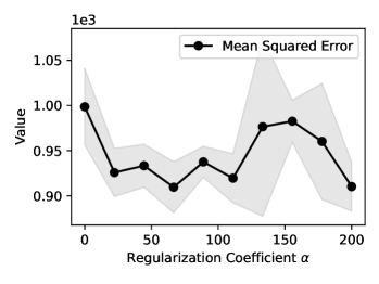
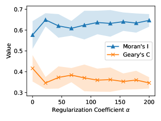
Figure 6. Sensitivity analysis of distance-preserving regularization strength in the performance.

We conduct further sensitivity analysis over our model’s regularization coefficient $\alpha$ to see its effects on the average MSE and the spatial correlation statistics. We use VAE as the backbone model and A2 as the testing dataset, and we evenly sample value from $0$ to $200$ to assign as our regularization coefficient. The other training parameters are set to be similar to the previous section. We plot the mean and standard deviation over five random trials in Figure 6 for each assigned regularization coefficient $\alpha$. We observe that the MSE plot (left) demonstrates a non-convex trend when increasing $\alpha$, but all $\alpha>0$ incurs a lower average MSE on the test dataset than without regularization ($\alpha=0$). The spatial autocorrelation plot (right) of Moran’s I and Geary’s C statistics shows a relatively positive trend with respect to $\alpha$. This indicates that a stronger distortion regularization can help the model effectively incorporate more spatial information into the latent representation.

As illustrated by the MSE plot (left) in Figure 6, incorporating more spatial information is not always helpful, as excessive emphasis on minimizing the distortion loss may hinder the model from placing enough attention towards capturing the internal structure that the gene expression itself exhibits. We suggest choosing the regularization parameter based on techniques such as cross-validation or prior knowledge of the data modeling objective.

6. Discussion

Our work has only limited the scope of study to the variational autoencoders, but there are also other generative models that have been incorporated into spatial transcriptomics modeling. For example, diffusion model (103, 2023; Mukhopadhyay et al., 2023) is another popular state-of-the-art generative model class. Recent works have developed new diffusion model architectures for spatial transcriptomics modeling tasks (Guo et al., 2024), including spatial transcriptomics prediction (Khan et al., 2024) and imputation (Li et al., 2024b). One may be interested in inspecting learning distance-preserving representations from denoising diffusion models (DDMs) (103, 2023; Mukhopadhyay et al., 2023) under the setting of spatial transcriptomics modeling. However, we note that an obstacle is that the representation capability of a DDM is not necessarily the outcome of its generation capability. The work by Chen et al. (2024) suggests that the representation capability of DDM is mainly gained by the denoising-driven process, not a diffusion-driven process.

While our work’s experimental evaluation has been limited in studying the reconstruction ability of the generative model, which is a straightforward way of inspecting the usefulness of latent representations, it is intriguing to know how distance-preserving may benefit many other tasks such as gene imputation or cell clustering.

Additionally, our sensitivity analysis has been confined to studying the regularization coefficient hyperparameters. We have also introduced the masking procedure at the end of Section 4.3. It is left to explore how choosing different scales of masking (e.g. the hyperparameter $k$ in K-NN) or masking procedure (using other clustering algorithms) would affect the learning outcome. Some preliminary analyses have been done on other works that study distance-preserving generative models, see e.g. (Chen et al., 2022).

Appendix A Proof of Lemma 4.2

Proof.

If $\mathcal{X}$ is a finite space or bounded space, then simply take:

$$M_{1}=\inf_{x,x^{\prime}\in\mathcal{X}}d_{\mathcal{X}}(x,x^{\prime}),\ M_{2}=\sup_{x,x^{\prime}\in\mathcal{X}}d_{\mathcal{X}}(x,x^{\prime}).$$

If $\mathcal{X}$ is an infinite space or an unbounded space, such as $\mathcal{X}=\mathbb{R}^{n}$. In this case, since we know that the Euclidean space $\mathbb{R}^{n}$ can be exhausted by a nested sequence of compact balls centered at the origin:

$$\mathcal{X}\subseteq\mathbb{R}^{n}=\bigcup_{r=1}^{+\infty}B(0,r),$$

where $B(0,r):=\left\{x\in\mathbb{R}^{n}:d_{\mathcal{X}}(x,0)\leq r\right\}$. Therefore, by the total probability property, we know that:

(12) $$\mathbb{P}(\mathcal{X})\leq\mathbb{P}\left(\bigcup_{r=1}^{+\infty}B(0,r)\right)=1.$$

By the dominated convergence theorem:

(13) $$\mathbb{P}\left(\lim_{R\to+\infty}\bigcup_{r=1}^{R}B(0,r)\right)=\lim_{R\to+\infty}\mathbb{P}\left(\bigcup_{r=1}^{R}B(0,r)\right).$$

By definition, given any $0<\delta<1$, there exists some $R^{\prime}>0$ such that:

$$\mathbb{P}\left(\bigcup_{r=1}^{R^{\prime}}B(0,r)\right)\geq 1-\delta,$$

which implies:

$$\mathbb{P}\left(-2R^{\prime}\leq|d_{\mathcal{X}}(x,x^{\prime})|\leq 2R^{\prime}\right)\geq 1-\delta.$$

Therefore, we can set $M_{1}=-2R^{\prime}$ and $M_{2}=2R^{\prime}$. This concludes the proof. ∎

Appendix B Proof of Theorem 4.3

Proof.

Denote the following events:

$$\mathcal{A} =\left\{M_{1}\leq\left|d_{\mathcal{X}}(x,x^{\prime})\right|\leq M_{2}\right\},$$

$$\mathcal{B} =\left\{\lambda d_{\mathcal{X}}(x,x^{\prime})-C\leq d_{\mathcal{Y}}\left(y,y^{\prime}\right)\leq\lambda d_{\mathcal{X}}(x,x^{\prime})+C\right\}$$

$$\mathcal{C} =\left\{\lambda d_{\mathcal{X}}(x,x^{\prime})\leq d_{\mathcal{Y}}\left(y,y^{\prime}\right)\leq L\cdot\lambda d_{\mathcal{X}}(x,x^{\prime})\right\},$$

Using Markov’s Inequality, for any $C>0$, we have:

$$\frac{\mathcal{L}_{\textrm{ISO}}}{C} \geq\mathbb{P}(\left|d_{\mathcal{Y}}(y,y^{\prime})-\lambda d_{\mathcal{X}}(x,x^{\prime})\right|\geq C).$$

Rearranging terms on both sides:

$$1-\frac{\mathcal{L}_{\textrm{ISO}}}{C}$$

$$\leq\mathbb{P}(\left|d_{\mathcal{Y}}(y,y^{\prime})-\lambda d_{\mathcal{X}}(x,x^{\prime})\right|\leq C)$$

$$=\mathbb{P}(\left|d_{\mathcal{Y}}(y,y^{\prime})-\lambda d_{\mathcal{X}}(x,x^{\prime})\right|\leq C)$$

$$=\mathbb{P}\left(\lambda d_{\mathcal{X}}(x,x^{\prime})-C\leq d_{\mathcal{Y}}\left(y,y^{\prime}\right)\leq\lambda d_{\mathcal{X}}(x,x^{\prime})+C\right)$$

(14) $$=\mathbb{P}(\mathcal{B})\addcontentsline{lla}{section}{\numberline{\string\crtrefnumber{eq:ineq}}{e}q:ineq}$$

If we set $L$ to satisfy:

(15) $$\addcontentsline{lla}{section}{\numberline{\string\crtrefnumber{eq:prop-3}}{e}q:prop-3}L=\frac{M_{2}}{M_{1}}+\frac{C}{\lambda M_{1}},$$

then it holds:

(16) $$\addcontentsline{lla}{section}{\numberline{\string\crtrefnumber{eq:prop-2}}{e}q:prop-2}\mathbb{P}(\mathcal{B}|\mathcal{A})\leq\mathbb{P}(\mathcal{C}|\mathcal{A}).$$

Using the law of total probability and the results we have derived, we can bound the probability of event $\mathcal{C}$ by:

$$\mathbb{P}(\mathcal{C}) =\mathbb{P}(\mathcal{C}|\mathcal{A})\mathbb{P}(\mathcal{A})+\mathbb{P}(\mathcal{C}|\mathcal{A}^{c})\mathbb{P}(\mathcal{A}^{c})$$

$$\geq\mathbb{P}(\mathcal{B}|\mathcal{A})(1-\delta)$$

$$\geq\mathbb{P}(\mathcal{B})-\delta$$

$$\geq 1-\mathcal{L}_{\textrm{ISO}}/{C}-\delta.$$

The first line uses the law of total probability, the second line uses (16) and Lemma 4.2, and the third line uses the law of total probability and Lemma 4.2:

$$\mathbb{P}(\mathcal{B}) =\mathbb{P}(\mathcal{B}|\mathcal{A})\mathbb{P}(\mathcal{A})+\mathbb{P}(\mathcal{B}|\mathcal{A}^{c})\mathbb{P}(\mathcal{A}^{c}),$$

$$\leq\mathbb{P}(\mathcal{B}|\mathcal{A})(1-\delta)+\delta$$

and the fourth line uses (14). Set $C=\mathcal{L}_{\textrm{ISO}}/(\varepsilon-\delta)$ and plug it into (15), we have:

$$L=\frac{M_{2}}{M_{1}}+\frac{\mathcal{L}_{\textrm{ISO}}}{\lambda M_{1}(\varepsilon-\delta)},$$

and:

$$\mathbb{P}\left(\lambda d_{\mathcal{X}}(x,x^{\prime})\leq d_{\mathcal{Y}}\left(y,y^{\prime}\right)\leq L\cdot\lambda d_{\mathcal{X}}(x,x^{\prime})\right)\geq 1-\varepsilon.$$

This proves $(L,\varepsilon)$-distortion as defined in Definition 4.1. The distortion constant satisfies by definition (8). ∎

Appendix C Additional Related Works

Spatial Data Modeling

Autoencoders have been widely utilized in the analysis of spatial data due to their powerful representation learning capabilities. Traditional autoencoders (AE) have been explored in several studies (Li et al., 2024a; Wan et al., 2023). For instance, SEDR (Xu et al., 2024) employs a deep auto-encoder network to learn gene representations while incorporating a variational graph auto-encoder to embed spatial information simultaneously, highlighting the integration of spatial and genetic data. The combination of autoencoders with graph neural networks (GNNs) has also proven effective, as shown in works by (Long et al., 2023; Zhou et al., 2023; Guo et al., 2023; Liu et al., 2023; Zhang et al., 2022), where such models enhance spatial data representation by leveraging graph structures. Additionally, advanced probabilistic models like the hidden Markov random field have been applied to spatial data, as demonstrated by Giotto (Dries et al., 2021b), which identifies spatial domains using an HMRF model with a spatial neighbor prior. This approach has been extended in studies like (Yang et al., 2022), further showcasing the potential of probabilistic methods in spatial data analysis.

Spatial Variational Autoencoders

Compared to the aforementioned approaches, variational autoencoders (VAEs) are recently attracting more attention in representation learning of single-cell data analysis (Du et al., 2022, 2020). They are preferred over traditional autoencoders because they provide a structured, continuous, and interpretable latent space that facilitates robust generative capabilities and handles uncertainty by explicitly modeling distributions. This results in more meaningful data generation and easier manipulation of latent features compared to traditional autoencoders, which can then be used for data integration (Du et al., 2022), trajectory inference (Du et al., 2020), etc. Furthermore, the study of VAEs lays the groundwork for extending methodologies to other variational inference-based models, such as diffusion models and variational graph autoencoders.

A series of works have been conducted to study the interplay of VAEs with spatial information in the data, and different variants of spatial VAEs have been proposed. (Bepler et al., 2019) enables learning VAE models of images that separate latent variables encoding content from rotation and translation. This can be done by directly constraining them as part of the latent space to be learned. (Wang et al., 2019) proposed to instead directly modify the latent space from the standard multi-variate Gaussian distributions to low-ranked matrix-variate normal distributions to allow for the better capturing ability of the spatial information present in image data. (guo, 2021) considered using VAE to learn disentangled representations of spatial networks via careful designs of the model structure and latent variable factorization. They proposed a tractable optimization algorithm to carry out variational learning. More recently, (Semenova et al., 2022) considered the setting of learning spatial Gaussian priors via variational autoencoder. (Hu et al., 2024) combined graph variational autoencoder with contrastive learning.

However, a critical distinct difference to be noted is that while most existing works studying spatial VAE aim to capture the representation of the spatial information, our work aims to refine the representation learned by incorporating the spatial information given as context. This is a different but equally challenging task with broad applications in fields where spatial information is easily accessible, such as spatial transcriptomics data analysis.

Appendix D Deriving ELBO of VAE

Below, we present the derivation of lower bound for the log probability density function (PDF) of VAE. To begin with, it can be written as:

$$\log f_{\theta}(y)=\log\int p_{\theta}(y,z)dz,$$

where $z$ is a latent random variable. This integral has no closed form and can be usually estimated by Monte Carlo integration with importance sampling, ie,

$$\int p_{\theta}(y,z)dz=\mathbb{E}_{z\sim q(\cdot|y)}\left[\frac{p_{\theta}(y,z)}{q(z|y)}\right].$$

Here $q(z|y)$ is the proposed variational distribution, where we can draw sample $z$ from this distribution given $y$ and $\mathbf{a}$. Therefore, by Jensen’s inequality, we can find evidence lower bound (ELBO) of the conditional PDF:

$$\log f_{\theta}(y) =\log\mathbb{E}_{z\sim q(\cdot|y)}\left[\frac{p_{\theta}(y,z)}{q(z|y)}\right]$$

$$\geq\mathbb{E}_{z\sim q(\cdot|y)}\left[\log\frac{p_{\theta}(y,z)}{q(z|y)}\right].$$

Using Bayes rule, the ELBO can be equivalently expressed as:

$$\mathbb{E}_{z\sim q(\cdot|y)}\left[\log\frac{p_{\theta}(y,z)}{q(z|y)}\right]$$

$$= \mathbb{E}_{z\sim q(\cdot|y)}\left[\log\frac{p_{\theta}(y|z)p_{\theta}(z)}{q(z|y)}\right]$$

$$= \mathbb{E}_{z\sim q(\cdot|y)}\left[\log\frac{p_{\theta}(z)}{q(z|y)}\right]+\mathbb{E}_{z\sim q(\cdot|y)}\left[\log p_{\theta}(y|z)\right]$$

$$= -D_{\text{KL}}(q(z|y)||p_{\theta}(z))+\mathbb{E}_{z\sim q(\cdot|y)}\left[\log p_{\theta}(y|z)\right].$$

This concludes the derivation.

Appendix E KL Divergence

Lemma E.1 (KL divergence of multivariate normals).

Suppose both $p$ and $q$ are the pdfs of multivariate normal distributions $\mathcal{N}_{d}(\bm{\mu}_{1},\bm{\Sigma}_{1})$ and $\mathcal{N}_{d}(\bm{\mu}_{2},\bm{\Sigma}_{2})$, respectively. The Kullback-Leibler distance from $p$ to $q$ is given by

$$D_{\text{KL}}(p||q)=\frac{1}{2}\left[\log\frac{|\bm{\Sigma}_{2}|}{|\bm{\Sigma}_{1}|}-d+\mathop{\mathrm{tr}}\{\bm{\Sigma}_{2}^{-1}\bm{\Sigma}_{1}\}\right.$$

$$\hskip 43.05542pt+\left.(\bm{\mu}_{2}-\bm{\mu}_{1})^{T}\bm{\Sigma}_{2}^{-1}(\bm{\mu}_{2}-\bm{\mu}_{1})\right].$$

When $\bm{\Sigma}_{1}={\rm diag}(\sigma_{1}^{2},\ldots,\sigma_{d}^{2})$ and $\bm{\Sigma}_{2}=\bm{I}_{d}$, it reduces to

$$D_{\text{KL}}(p||q)=-\frac{1}{2}\left[d+\sum_{j=1}^{d}\log\sigma_{j}^{2}-\sum_{j=1}^{d}\sigma_{j}^{2}-\|\bm{\mu}_{2}-\bm{\mu}_{1}\|_{2}^{2}\right].$$

Proof of Lemma E.1.

By definition, we have

$$D_{\text{KL}}(p||q) =\int\left[\log(p(\bm{x}))-\log(q(\bm{x}))\right]\ p(\bm{x}){\,\mathrm{d}}\bm{x}$$

$$=\int\left[\frac{1}{2}\log\frac{|\bm{\Sigma}_{2}|}{|\bm{\Sigma}_{1}|}-\frac{1}{2}(x-\bm{\mu}_{1})^{T}\bm{\Sigma}_{1}^{-1}(x-\bm{\mu}_{1})\right.$$

$$\quad+\left.\frac{1}{2}(x-\bm{\mu}_{2})^{T}\bm{\Sigma}_{2}^{-1}(x-\bm{\mu}_{2})\right]p(x){\,\mathrm{d}}x$$

$$=\frac{1}{2}\log\frac{|\bm{\Sigma}_{2}|}{|\bm{\Sigma}_{1}|}-\frac{1}{2}\mathop{\mathrm{tr}}\ \left\{\mathbb{E}[(x-\bm{\mu}_{1})(x-\bm{\mu}_{1})^{T}]\ \bm{\Sigma}_{1}^{-1}\right\}$$

$$\quad+\frac{1}{2}\mathbb{E}[(x-\bm{\mu}_{2})^{T}\bm{\Sigma}_{2}^{-1}(x-\bm{\mu}_{2})]$$

$$=\frac{1}{2}\log\frac{|\bm{\Sigma}_{2}|}{|\bm{\Sigma}_{1}|}-\frac{1}{2}\mathop{\mathrm{tr}}\ \{I_{d}\}+\frac{1}{2}(\bm{\mu}_{1}-\bm{\mu}_{2})^{T}\bm{\Sigma}_{2}^{-1}(\bm{\mu}_{1}-\bm{\mu}_{2})$$

$$+\frac{1}{2}\mathop{\mathrm{tr}}\{\bm{\Sigma}_{2}^{-1}\bm{\Sigma}_{1}\}$$

The last expression on the right-hand side translates to:

$$\frac{1}{2}\left[\log\frac{|\bm{\Sigma}_{2}|}{|\bm{\Sigma}_{1}|}-d+\mathop{\mathrm{tr}}\{\bm{\Sigma}_{2}^{-1}\bm{\Sigma}_{1}\}+(\bm{\mu}_{2}-\bm{\mu}_{1})^{T}\bm{\Sigma}_{2}^{-1}(\bm{\mu}_{2}-\bm{\mu}_{1})\right],$$

which finishes the proof. ∎

Appendix F Additional Experiment Details

KL Weight

Adjusting for the KL weight makes the model a $\beta$-VAE (Higgins et al., 2017). Specifically, its ELBO loss is defined as:

$$-\beta\cdot D_{\text{KL}}(q(z|y)||p_{\theta}(z))+\mathbb{E}_{z\sim q(\cdot|y)}\left[\log p_{\theta}(y|z)\right],$$

where $\beta$ is a hyperparameter that controls the weight of the KL term in the ELBO loss function. Intuitively, a larger KL weight forces the VAE to confine to the prior distribution more, and a smaller KL weight allows the VAE to focus more on minimizing the reconstruction loss. In our experiments, since Gaussian prior is a prohibitive assumption, we would want to lower its weight to ensure that the extracted latent representation is meaningful.

Network configuration of VAE

The neural network layers of the VAE model that we implemented using PyTorch (Paszke et al., 2019). The hidden layer consists of a fully connected layer and a LeakyReLU activation layer.

Moran’s I and Geary’s C

Moran’s I metric (Li et al., 2007) is a correlation coefficient that measures the overall spatial autocorrelation of a dataset. Intuitively, for a given gene, it measures how one spot is similar to others surrounding it. If the spots are attracted (or repelled) by each other, it implies they are not independent. Thus, the presence of autocorrelation indicates the spatial pattern of gene expression. Moran’s I value ranges from –1 to 1, where a value close to 1 indicates a clear spatial pattern, a value close to 0 indicates random spatial expression, and a value close to –1 indicates a chessboard-like pattern. To evaluate the spatial variability of a given gene, we calculate the Moran’s I using the following formula,

$$I=\frac{N}{W}\frac{\sum_{i}\sum_{j}\left[w_{ij}\left(x_{i}-\bar{x}\right)\left(x_{j}-\bar{x}\right)\right]}{\sum_{i}\left(x_{i}-\bar{x}\right)^{2}},$$

where $x_{i}$ and $x_{j}$ are the gene expression of spots $i$ and $j$, $\bar{x}$ is the mean expression of the feature, $N$ is the total number of spots, $w_{ij}$ is the spatial weight between spots $i$ and $j$ calculated using the 2D spatial coordinates of the spots, and $W$ is the sum of $w_{ij}$. We select the $k$ nearest neighbors for each spot using spatial coordinates. Moran’s I statistic is robust to the choice of $k$ and is set at 5 in our analysis. We assign $w_{ij}=1$ if spot $j$ is in the nearest neighbors of spot $i$, and 0 otherwise.

Geary’s $C$ is another commonly used statistic for measuring spatial autocorrelation. It is calculated as:

$$C=\frac{N-1}{2W}\frac{\sum_{i}\sum_{j}\left[w_{ij}\left(x_{i}-x_{j}\right)^{2}\right]}{\sum_{i}\left(x_{i}-\bar{x}\right)^{2}},$$

The value of Geary’s $C$ ranges from zero to two, where zero indicates perfect positive autocorrelation.

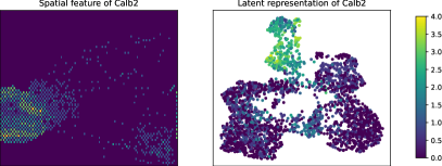
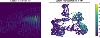
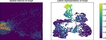
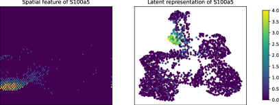
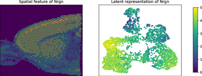
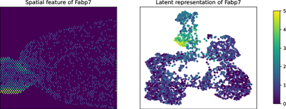
Figure 7. Latent representation extracted from VAE trained on the Mouse Brain Serial Datasets anterior 1. The olfactory bulb region, with genes Calb2, Gng4, S100a5, and Febp7 enriched, is well separated from other regions

Marker gene expression latent representation

Figure 7 shows the gene expression levels of six marker genes extracted by VAE. For each gene in each panel, the left subplot shows the gene expression levels in the spatial coordinates, and the right subplot shows the 2D-UMAP of the latent representation of the corresponding model. As we can see, the cells are dispersed in the latent space. The olfactory bulb region, with genes Calb2, Gng4, S100a5, and Febp7 enriched, is well separated from other regions.

References

- (1)
- guo (2021) 2021. Deep generative models for spatial networks.
- 103 (2023) 2023. Denoising Diffusion Autoencoders are Unified Self-supervised Learners. IEEE Computer Society, Los Alamitos, CA, USA.
- Benaim and Wolf (2017) Sagie Benaim and Lior Wolf. 2017. One-sided unsupervised domain mapping. Advances in neural information processing systems 30 (2017).
- Bengio and LeCun (2014) Yoshua Bengio and Yann LeCun (Eds.). 2014. Auto-Encoding Variational Bayes.
- Bepler et al. (2019) Tristan Bepler, Ellen Zhong, Kotaro Kelley, Edward Brignole, and Bonnie Berger. 2019. Explicitly disentangling image content from translation and rotation with spatial-VAE. Advances in Neural Information Processing Systems 32 (2019).
- Beshkov et al. (2022) Kosio Beshkov, Jonas Verhellen, and Mikkel Elle Lepperød. 2022. Isometric Representations in Neural Networks Improve Robustness. arXiv preprint arXiv:2211.01236 (2022).
- Chen et al. (2022) Nutan Chen, Patrick van der Smagt, and Botond Cseke. 2022. Local distance preserving auto-encoders using continuous knn graphs. In Topological, Algebraic and Geometric Learning Workshops 2022. PMLR, 55–66.
- Chen et al. (2023) Tsai-Ying Chen, Li You, Jose Angelito U Hardillo, and Miao-Ping Chien. 2023. Spatial transcriptomic technologies. Cells 12, 16 (2023), 2042.
- Chen et al. (2024) Xinlei Chen, Zhuang Liu, Saining Xie, and Kaiming He. 2024. Deconstructing Denoising Diffusion Models for Self-Supervised Learning. arXiv preprint arXiv:2401.14404 (2024).
- Chennuru Vankadara and von Luxburg (2018) Leena Chennuru Vankadara and Ulrike von Luxburg. 2018. Measures of distortion for machine learning. Advances in Neural Information Processing Systems 31 (2018).
- Dries et al. (2021a) Ruben Dries, Jiaji Chen, Natalie Del Rossi, Mohammed Muzamil Khan, Adriana Sistig, and Guo-Cheng Yuan. 2021a. Advances in spatial transcriptomic data analysis. Genome research 31, 10 (2021), 1706–1718.
- Dries et al. (2021b) Ruben Dries, Qian Zhu, Rui Dong, Chee-Huat Linus Eng, Huipeng Li, Kan Liu, Yuntian Fu, Tianxiao Zhao, Arpan Sarkar, Feng Bao, et al. 2021b. Giotto: a toolbox for integrative analysis and visualization of spatial expression data. Genome biology 22 (2021), 1–31.
- Du et al. (2022) Jin-Hong Du, Zhanrui Cai, and Kathryn Roeder. 2022. Robust probabilistic modeling for single-cell multimodal mosaic integration and imputation via scVAEIT. Proceedings of the National Academy of Sciences 119, 49 (2022), e2214414119.
- Du et al. (2020) Jin-Hong Du, Tianyu Chen, Ming Gao, and Jingshu Wang. 2020. Joint Trajectory Inference for Single-cell Genomics Using Deep Learning with a Mixture Prior. bioRxiv (2020), 2020–12.
- Edsgärd et al. (2018) Daniel Edsgärd, Per Johnsson, and Rickard Sandberg. 2018. Identification of spatial expression trends in single-cell gene expression data. Nature methods 15, 5 (2018), 339–342.
- Guo et al. (2023) Tiantian Guo, Zhiyuan Yuan, Yan Pan, Jiakang Wang, Fengling Chen, Michael Q Zhang, and Xiangyu Li. 2023. SPIRAL: integrating and aligning spatially resolved transcriptomics data across different experiments, conditions, and technologies. Genome Biology 24, 1 (2023), 241.
- Guo et al. (2024) Zhiye Guo, Jian Liu, Yanli Wang, Mengrui Chen, Duolin Wang, Dong Xu, and Jianlin Cheng. 2024. Diffusion models in bioinformatics and computational biology. Nature reviews bioengineering 2, 2 (2024), 136–154.
- Hadsell et al. (2006) Raia Hadsell, Sumit Chopra, and Yann LeCun. 2006. Dimensionality reduction by learning an invariant mapping. In 2006 IEEE computer society conference on computer vision and pattern recognition (CVPR’06), Vol. 2. IEEE, 1735–1742.
- Hao et al. (2023) Yuhan Hao, Tim Stuart, Madeline H Kowalski, Saket Choudhary, Paul Hoffman, Austin Hartman, Avi Srivastava, Gesmira Molla, Shaista Madad, Carlos Fernandez-Granda, et al. 2023. Dictionary learning for integrative, multimodal and scalable single-cell analysis. Nature Biotechnology (2023), 1–12.
- Higgins et al. (2017) Irina Higgins, Loic Matthey, Arka Pal, Christopher P Burgess, Xavier Glorot, Matthew M Botvinick, Shakir Mohamed, and Alexander Lerchner. 2017. beta-vae: Learning basic visual concepts with a constrained variational framework. ICLR (Poster) 3 (2017).
- Hu et al. (2021) Jian Hu, Xiangjie Li, Kyle Coleman, Amelia Schroeder, Nan Ma, David J Irwin, Edward B Lee, Russell T Shinohara, and Mingyao Li. 2021. SpaGCN: Integrating gene expression, spatial location and histology to identify spatial domains and spatially variable genes by graph convolutional network. Nature methods 18, 11 (2021), 1342–1351.
- Hu et al. (2024) Yaofeng Hu, Kai Xiao, Hengyu Yang, Xiaoping Liu, Chuanchao Zhang, and Qianqian Shi. 2024. Spatially contrastive variational autoencoder for deciphering tissue heterogeneity from spatially resolved transcriptomics. Briefings in Bioinformatics 25, 2 (2024), bbae016.
- Khan et al. (2024) Sumeer Ahmad Khan, Vincenzo Lagani, Robert Lehmann, Narsis A Kiani, David Gomez-Cabrero, and Jesper Tegner. 2024. SpatialDiffusion: Predicting Spatial Transcriptomics with Denoising Diffusion Probabilistic Models. bioRxiv (2024), 2024–05.
- Kim et al. (2020) Chelhwon Kim, Andrew Port, and Mitesh Patel. 2020. Face-to-Music Translation Using a Distance-Preserving Generative Adversarial Network with an Auxiliary Discriminator. arXiv preprint arXiv:2006.13469 (2020).
- Lee et al. (2021) Yonghyeon Lee, Hyeokjun Kwon, and Frank Park. 2021. Neighborhood reconstructing autoencoders. Advances in Neural Information Processing Systems 34 (2021), 536–546.
- Li et al. (2007) Hongfei Li, Catherine A Calder, and Noel Cressie. 2007. Beyond Moran’s I: testing for spatial dependence based on the spatial autoregressive model. Geographical analysis 39, 4 (2007), 357–375.
- Li et al. (2024b) Kongming Li, Jiahao Li, Yuhao Tao, and Fei Wang. 2024b. stDiff: a diffusion model for imputing spatial transcriptomics through single-cell transcriptomics. Briefings in Bioinformatics 25, 3 (2024), bbae171.
- Li et al. (2024a) Shang Li, Kuo Gai, Kangning Dong, Yiyang Zhang, and Shihua Zhang. 2024a. High-density generation of spatial transcriptomics with STAGE. Nucleic Acids Research (2024), gkae294.
- Liu et al. (2023) Teng Liu, Zhao-Yu Fang, Zongbo Zhang, Yongxiang Yu, Min Li, and Ming-Zhu Yin. 2023. A comprehensive overview of graph neural network-based approaches to clustering for spatial transcriptomics T. Liu et al. Overview of Spatial Transcriptomics’ Spatial Clutering. Computational and Structural Biotechnology Journal (2023).
- Long et al. (2023) Yahui Long, Kok Siong Ang, Mengwei Li, Kian Long Kelvin Chong, Raman Sethi, Chengwei Zhong, Hang Xu, Zhiwei Ong, Karishma Sachaphibulkij, Ao Chen, et al. 2023. Spatially informed clustering, integration, and deconvolution of spatial transcriptomics with GraphST. Nature Communications 14, 1 (2023), 1155.
- Lopez et al. (2019) Romain Lopez, Achille Nazaret, Maxime Langevin, Jules Samaran, Jeffrey Regier, Michael I Jordan, and Nir Yosef. 2019. A joint model of unpaired data from scRNA-seq and spatial transcriptomics for imputing missing gene expression measurements. arXiv preprint arXiv:1905.02269 (2019).
- Lopez et al. (2018) Romain Lopez, Jeffrey Regier, Michael B Cole, Michael I Jordan, and Nir Yosef. 2018. Deep generative modeling for single-cell transcriptomics. Nature methods 15, 12 (2018), 1053–1058.
- Mahabadi et al. (2018) Sepideh Mahabadi, Konstantin Makarychev, Yury Makarychev, and Ilya Razenshteyn. 2018. Nonlinear dimension reduction via outer bi-lipschitz extensions. In Proceedings of the 50th Annual ACM SIGACT Symposium on Theory of Computing. 1088–1101.
- Mao et al. (2019) Chengzhi Mao, Ziyuan Zhong, Junfeng Yang, Carl Vondrick, and Baishakhi Ray. 2019. Metric learning for adversarial robustness. Advances in neural information processing systems 32 (2019).
- McInnes et al. (2018) Leland McInnes, John Healy, Nathaniel Saul, and Lukas Großberger. 2018. UMAP: Uniform Manifold Approximation and Projection. Journal of Open Source Software 3, 29 (2018).
- Mukhopadhyay et al. (2023) Soumik Mukhopadhyay, Matthew Gwilliam, Vatsal Agarwal, Namitha Padmanabhan, Archana Swaminathan, Srinidhi Hegde, Tianyi Zhou, and Abhinav Shrivastava. 2023. Diffusion models beat gans on image classification. arXiv preprint arXiv:2307.08702 (2023).
- Paszke et al. (2019) Adam Paszke, Sam Gross, Francisco Massa, Adam Lerer, James Bradbury, Gregory Chanan, Trevor Killeen, Zeming Lin, Natalia Gimelshein, Luca Antiga, et al. 2019. Pytorch: An imperative style, high-performance deep learning library. Advances in neural information processing systems 32 (2019).
- Port et al. (2020) Andrew Port, Chelhwon Kim, and Mitesh Patel. 2020. Earballs: Neural transmodal translation. arXiv preprint arXiv:2005.13291 1 (2020).
- Semenova et al. (2022) Elizaveta Semenova, Yidan Xu, Adam Howes, Theo Rashid, Samir Bhatt, Swapnil Mishra, and Seth Flaxman. 2022. PriorVAE: encoding spatial priors with variational autoencoders for small-area estimation. Journal of the Royal Society Interface 19, 191 (2022), 20220094.
- Sohn et al. (2015) Kihyuk Sohn, Honglak Lee, and Xinchen Yan. 2015. Learning structured output representation using deep conditional generative models. Advances in neural information processing systems 28 (2015).
- Sun et al. (2020) Shiquan Sun, Jiaqiang Zhu, and Xiang Zhou. 2020. Statistical analysis of spatial expression patterns for spatially resolved transcriptomic studies. Nature methods 17, 2 (2020), 193–200.
- Svensson et al. (2018) Valentine Svensson, Sarah A Teichmann, and Oliver Stegle. 2018. SpatialDE: identification of spatially variable genes. Nature methods 15, 5 (2018), 343–346.
- Verine et al. (2023) Alexandre Verine, Benjamin Negrevergne, Yann Chevaleyre, and Fabrice Rossi. 2023. On the expressivity of bi-Lipschitz normalizing flows. In Asian Conference on Machine Learning. PMLR, 1054–1069.
- Wan et al. (2023) Xiaomeng Wan, Jiashun Xiao, Sindy Sing Ting Tam, Mingxuan Cai, Ryohichi Sugimura, Yang Wang, Xiang Wan, Zhixiang Lin, Angela Ruohao Wu, and Can Yang. 2023. Integrating spatial and single-cell transcriptomics data using deep generative models with SpatialScope. Nature Communications 14, 1 (2023), 7848.
- Wang et al. (2019) Zhengyang Wang, Hao Yuan, and Shuiwang Ji. 2019. Spatial Variational Auto-Encoding via Matrix-Variate Normal Distributions. In Proceedings of the 2019 SIAM International Conference on Data Mining. SIAM, 648–656.
- Wu et al. (2023) Shenghao Wu, Wenbin Zhou, Minshuo Chen, and Shixiang Zhu. 2023. Counterfactual Generative Models for Time-Varying Treatments. arXiv preprint arXiv:2305.15742 (2023).
- Xu et al. (2024) Hang Xu, Huazhu Fu, Yahui Long, Kok Siong Ang, Raman Sethi, Kelvin Chong, Mengwei Li, Rom Uddamvathanak, Hong Kai Lee, Jingjing Ling, et al. 2024. Unsupervised spatially embedded deep representation of spatial transcriptomics. Genome Medicine 16, 1 (2024), 12.
- Yang et al. (2022) Yi Yang, Xingjie Shi, Wei Liu, Qiuzhong Zhou, Mai Chan Lau, Jeffrey Chun Tatt Lim, Lei Sun, Cedric Chuan Young Ng, Joe Yeong, and Jin Liu. 2022. SC-MEB: spatial clustering with hidden Markov random field using empirical Bayes. Briefings in bioinformatics 23, 1 (2022), bbab466.
- Yonghyeon et al. (2021) LEE Yonghyeon, Sangwoong Yoon, Minjun Son, and Frank C Park. 2021. Regularized autoencoders for isometric representation learning. In International Conference on Learning Representations.
- Yu et al. (2022) Qichao Yu, Miaomiao Jiang, and Liang Wu. 2022. Spatial transcriptomics technology in cancer research. Frontiers in Oncology 12 (2022), 1019111.
- Zeng et al. (2022) Zexian Zeng, Yawei Li, Yiming Li, and Yuan Luo. 2022. Statistical and machine learning methods for spatially resolved transcriptomics data analysis. Genome biology 23, 1 (2022), 83.
- Zhang et al. (2022) Xinyi Zhang, Xiao Wang, GV Shivashankar, and Caroline Uhler. 2022. Graph-based autoencoder integrates spatial transcriptomics with chromatin images and identifies joint biomarkers for Alzheimer’s disease. Nature Communications 13, 1 (2022), 7480.
- Zhou et al. (2023) Xiang Zhou, Kangning Dong, and Shihua Zhang. 2023. Integrating spatial transcriptomics data across different conditions, technologies and developmental stages. Nature Computational Science 3, 10 (2023), 894–906.
- Zhu and Sabatti (2020) Junjie Zhu and Chiara Sabatti. 2020. Integrative spatial single-cell analysis with graph-based feature learning. Biorxiv (2020), 2020–08.
- Zhu et al. (2021) Jiaqiang Zhu, Shiquan Sun, and Xiang Zhou. 2021. SPARK-X: non-parametric modeling enables scalable and robust detection of spatial expression patterns for large spatial transcriptomic studies. Genome biology 22, 1 (2021), 184.