GRADIENT-FREE OPTIMIZATION VIA INTEGRATION

Abstract. In this paper we propose a novel, general purpose, algorithm to optimize functions $l\colon\mathbb{R}^{d}\rightarrow\mathbb{R}$ not assumed to be convex or differentiable or even continuous. The main idea is to sequentially fit a sequence of parametric probability densities, possessing a concentration property, to $l$ using a Bayesian update followed by a reprojection back onto the chosen parametric sequence. Remarkably, with the sequence chosen to be from the exponential family, reprojection essentially boils down to the computation of expectations. Our algorithm therefore lends itself to Monte Carlo approximation, ranging from plain to Sequential Monte Carlo (SMC) methods. The algorithm is therefore particularly simple to implement and we illustrate performance on a challenging Machine Learning classification problem. Our methodology naturally extends to the scenario where only noisy measurements of $l$ are available and retains ease of implementation and performance. At a theoretical level we establish, in a fairly general scenario, that our framework can be viewed as implicitly implementing a time inhomogeneous gradient descent algorithm on a sequence of smoothed approximations of $l$. This opens the door to establishing convergence of the algorithm and provide theoretical guarantees. Along the way, we establish new results for inhomogeneous gradient descent algorithms of independent interest.

Keywords: Gradient-Free Optimisation, Sequential Monte Carlo, Bayesian Updating, Variational methods, Smoothing.

All notation can be found in Appendix A.

1 Introduction

Let $l\colon\mathsf{X}:=\mathbb{R}^{d}\rightarrow\mathbb{R}$ be a lower-semicontinuous, potentially non-differentiable function such that $\inf_{x\in\mathbb{R}^{d}}l(x)>-\infty$ and hence $\arg\min_{x\in K}l(x)\neq\varnothing$ for any compact set $K\subset\mathsf{X}$. This manuscript is concerned with gradient free algorithms to minimize functions within this class, both in the scenario where $l$ can be evaluated pointwise or only unbiased and independent noisy measurements are available, formalised as $l(x):=\mathbb{E}(\ell(x,U))$ for $U\in\mathsf{U}$ drawn from a distribution independent of $x\in\mathbb{R}^{d}$, where $\ell\colon\mathbb{R}^{d}\times\mathsf{U\rightarrow\mathbb{R}}$ can be evaluated pointwise.

Noiseless scenario

In the scenario where $l(\cdot)$ can be evaluated pointwise, the main idea of the class of algorithms we propose can be easily understood with the following particular example. Let $\phi_{d}$ be the density of the standard normal distribution $\mathcal{N}(0,\mathbf{I}_{d})$ and define $\pi_{\theta,\gamma}(x):=\gamma^{-d/2}\phi_{d}\big{(}\gamma^{-1/2}(x-\theta)\big{)}$ for $\theta\in\Theta=\mathbb{R}^{d}$, $\gamma>0$. Then, for a sequence $\{\gamma_{n}\geq 0,n\in\mathbb{N}\}$ such that $\gamma_{n}\downarrow 0$ define sequentially the families of distributions $\{\pi_{n},n\in\mathbb{N}\}$ and $\{\tilde{\pi}_{n},n\in\mathbb{N}\}$ as in Alg. 1.

Algorithm 1 Deterministic Gradient-Free Ideal Algorithm

$x\mapsto l(x)$ $\triangleright$ objective function

$\theta_{0}$, $\{\gamma_{k},k\geq 0\}$$\triangleright$ initial value and stepsizes

$\pi_{0}(x)=\pi_{\theta_{0},\gamma_{0}}(x)$ $\triangleright$ initial distribution

while $n\geq 0$ do

    $\tilde{\pi}_{n+1}(x)\propto\exp(-l(x))\pi_{n}(x)$ $\triangleright$ generalised bayesian rule

    $\theta_{n+1}\in\operatorname*{argmin}_{\theta\in\Theta}\mathcal{\mathrm{KL}}(\tilde{\pi}_{n+1},\pi_{\theta,\gamma_{n}})$ $\triangleright$ project with Kullback-Leibler divergence

    Set $\pi_{n+1}=\pi_{\theta_{n+1},\gamma_{n+1}}$ $\triangleright$ distribution shrinking

end while

sequence of distributions $\tilde{\pi}_{n}$ and parameters $\theta_{n}$.

An iteration of Alg. 1 therefore consists of the application of Bayes’ rule, where $l(\cdot)$ plays the role of a negative log-likelihood and $\pi_{n}$ that of the prior distribution, followed by a “projection” onto the normal family $\pi_{\theta,\gamma_{n}}$, using the Kullback-Leibler divergence as a criterion. In a standard statistical context, repeated application of Bayes’ rule, in the scenario involving random data, is known to lead to a concentration phenomenon around particular maximum points or the posteriors, under general conditions Kleijn and van der Vaart, (2012); a similar phenomenon occurs in the present setup and is illustrated in Fig. 1.

Remark 1.1.

In practice, one may approximate Alg. 1 by replacing $\tilde{\pi}_{n}$ with a cloud of $N\in\mathbb{N}$ weighted random samples $\{X_{n}^{i},i\in\llbracket N\rrbracket\}$ propagated along the iterations;see Section 2 for details. The rest of the paper (Section 3 onwards) focuses on ideal algorithms, corresponding to the scenario $N\rightarrow\infty$. We see the study of such ideal algorithms as a prerequisite to the study of their implementable versions, seen as perturbations of the ideal algorithms.

Figure 1: Illustration of the algorithm in the Gaussian case. The initial Gaussian density (light red, $n=0$) is multiplied with $\exp(-l(\cdot))$, where $l(x)=x^{2}$ (blue in the background). The product is not shown but fitted with another Gaussian using the KL divergence and assigned a smaller variance. The multiplication operation gives more weight to the points close to the maximum of $\exp(-l(\cdot))$ - that is, close to the minimum of $l(\cdot)$. As a result the Gaussians (red to black) are attracted to regions of low values of $l(\cdot)$. Together with shrinking of the covariance results this in concentration minimum of $l(\cdot)$. Note that differentiability of $l(\cdot)$ is not used here.

The update considered here differs from standard Bayesian updating in that it involves a reprojection step, therefore necessitating a new approach to establishing ability of the algorithm to find minima of $l(\cdot)$. This reprojection step is motivated by practical considerations. Indeed it circumvents the need to propagate the sequence of distributions obtained by repeated use of Bayes’ update and greatly facilitates implementation. It turns out that this reprojection step also facilitates theoretical analysis. Indeed the crucial observation allowing us to prove convergence of Alg. 1, in the sense that $\pi_{n}$ concentrates on local minima of $l(\cdot)$, is that it implicitly implements a steepest descent algorithm tracking the minima of a sequence of differentiable approximations $\{h_{n}\colon\mathbb{R}^{d}\rightarrow\mathbb{R},n\geq 1\}$ of $l(\cdot)$. When such approximations converge to $l(\cdot)$, validity of the procedure should ensue.

More precisely, the reprojection step can be shown to correspond to so-called moment matching, a fact extensively used in variational inference Wainwright and Jordan, (2008). Taking into account that in the present setup $\theta_{n+1}$ is the first order moment of $\pi_{n+1}$, or mean, moment matching takes the form

$$\theta_{n+1}=\int x\tilde{\pi}_{n+1}(x){\mathrm{d}}x=\theta_{n}+\frac{\int(x-\theta_{n})\exp\big{(}-l(x)\big{)}\phi\big{(}\frac{x-\theta_{n}}{\sqrt{\gamma_{n}}}\big{)}{\mathrm{d}}x}{\int\exp\big{(}-l(x)\big{)}\phi\big{(}\frac{x-\theta_{n}}{\sqrt{\gamma_{n}}}\big{)}{\mathrm{d}}x}\,.$$ (1)

It is the evaluation of these expectations which in practice requires a Monte Carlo approximation with weighted samples. For $(\theta,\gamma)\in\Theta\times\mathbb{R}_{+}$ let

$$h_{\gamma}(\theta):=-\log\left(\int\exp\big{(}-l(x)\big{)}\phi\Bigl{(}\frac{x-\theta}{\sqrt{\gamma}}\Bigr{)}{\mathrm{d}}x\right)\,,$$

and for $n\in\mathbb{N}$ and $\theta\in\Theta$ let $h_{n}(\theta):=h_{\gamma_{n}}(\theta).$ Then one can write (1) in the familiar form

$$\theta_{n+1}=\theta_{n}-\gamma_{n}\nabla h_{n}(\theta_{n})\,,$$ (2)

and recognize a time inhomogeneous steepest-descent algorithm tracking the sequence of stationary points of the sequence of functions $\{h_{n},n\in\mathbb{N}\}$, again smoothed versions of $l(\cdot)$. It should be remarkable that while this interpretation provides us with an additional rational for Alg. 1 and a route to establishing its convergence for a large class of non-differentiable functions $l(\cdot)$ (the subject of Section 3), implementation does not require differentiation but instead integration.

The arguments we provide in Sections 3 and 4 lead to the following convergence result on the inhomogeneous gradient descent in (2). We again remark that, due to the equivalence, this in fact represents a convergence result for Alg. 1 where at every iteration one reprojects on the Gaussian family by minimisation of the Kullback-Leibler divergence.

Theorem 1.1.

Let $l:\mathbb{R}^{d}\to\mathbb{R}$ be lower-bounded, strongly lower-semicontinuous and assume there exists $C_{l}\in(0,\infty)$ such that $|l(\theta^{\prime})-l(\theta)|\leq C_{l}+C_{l}\|\theta-\theta^{\prime}\|^{2}$ for all $\theta,\theta^{\prime}\in\mathbb{R}^{d}$. Let $\{\gamma_{n},\,n\in\mathbb{N}\}$ be a sequence with $\gamma_{n}=n^{-\beta}$ for all $n\geq 1$, for some $\beta\in(0,1)$. Let $\left\{\theta_{n},\,n\in\mathbb{N}\right\}$ be the output of recursion (2), corresponding to Alg. 1. Then, there exists a subsequence $\left\{\theta_{n_{k}},\,k\in\mathbb{N}\right\}$ of $\{\theta_{n},\,n\in\mathbb{N}\}$ such that $\lim_{k\rightarrow\infty}\|\nabla h_{n_{k}}(\theta_{n_{k}})\|=0$.

We see that the most stringent assumptions on $l(\cdot)$ is simply that its ‘jumps’ are bounded and that its variations are at most quadratic for large increments of $\theta$. This condition is always satisfied for $l(\cdot)$ bounded. When combined with the characterisation of local minima (Theorem 3.2) in our framework, Theorem 1.1 constitutes a tool to identify local minima candidates. In particular, as will shall see, this theorem implies that if the sequence $\left\{\theta_{n},\,n\in\mathbb{N}\right\}$ defined in Alg. 1 converges to some $\theta$ then $\theta$ is a candidate for a local minima of $l(\cdot)$. Theorem 1.1 therefore provides a convergence result for Alg. 1 under mild assumptions on $l(\cdot)$, but it also leads to a number of consequences and stronger results, when more is known on the objective function. For instance, when $x\mapsto l(x)$ is convex, the functions $\theta\mapsto h_{n}(\theta)$ are also convex for $n\in\mathbb{N}$: in this case, one can easily show that Alg. 1 converges to the minimiser of $l(\cdot)$.

Beyond standard mollifiers

Readers interested in implementation and algorithm performance may jump to Section 3 on a first reading. The notion of mollifiers is precisely defined in Def. 4.1. An important point is that the above examples relying on $\pi_{\theta,\gamma}$ being a normal distribution of known covariance matrix is a particular case of a more general class of algorithms we introduce and study in this manuscript. Consider now the scenario where $\pi_{\theta,\gamma}$ in Alg. 1 belongs to the regular exponential dispersion models (EDM) family of distributions Jorgensen, (1987, 1997); for the reader’s convenience we provide standard background implicitly used below in Appendix B.1. Such models are of the form

$$\pi_{\theta,\gamma}(x)=\eta(\gamma,x)\exp\left\{\gamma^{-1}\big{[}\langle\theta,T(x)\rangle-A(\theta)\big{]}\right\}\,,$$

where $T\colon\mathsf{X}\rightarrow\mathsf{T}$ and $\theta\in\Theta$. The normal distribution used earlier is a particular instance of this family and other examples include the Gamma distribution or the Wishart distribution among others. The motivation behind EDMs in the present context is that, provided $\theta\rightarrow A(\theta)$ is twice differentiable

$$\mu(\theta):=\mathbb{E}_{\pi_{\theta,\gamma}}\big{(}T(X)\big{)}=\nabla_{\theta}A(\theta)$$

$$\mathrm{var}_{\pi_{\theta,\gamma}}\big{(}T(X)\big{)}=\gamma\nabla_{\theta}^{2}A(\theta)\,.$$

This is interesting for the following reason: for any $\theta\in\Theta$, letting $\gamma\downarrow 0$ ensures that the distribution of $T(X)$ under $\pi_{\theta,\gamma}$ concentrates on $\mu(\theta)$. In the most common scenario where $T(x)=x$ (or a component of $T(x)$ is $x$), which is the case of the normal example we started with, this means that whenever $\theta\mapsto\mu(\theta)$ spans $\mathsf{X}$ then we can aim to adjust $\theta$ to ensure $\mu(\theta)\in\arg\min_{x\in\mathsf{X}}l(x)$. In the more general scenario, we may have $l(x)=\check{l}\circ T(x)$ for some $\check{l}\colon\mathsf{T}\rightarrow\mathbb{R}$; this is illustrated in Subsection B.4 in the scenario where one wants $\pi_{\theta,\gamma}$ to be a Beta distribution.

An interesting point is that such a search of a suitable $\theta$ is achieved with Alg. 1, without any modification and the gradient descent justification still holds. Notice first that the Bayes’ update

$$\tilde{\pi}_{\theta,\gamma}(x)=\tilde{\eta}(\gamma,x)\exp\left\{\gamma^{-1}\big{[}\langle\theta,T(x)\rangle-\tilde{A}(\theta)\big{]}\right\}\,,$$

is of a form similar to $\pi_{\theta,\gamma}$ with $\tilde{\eta}(\gamma,x)=\exp\big{(}-l(x)\big{)}\eta(\gamma,x)$ and $\tilde{A}(\theta)=A(\theta)+\gamma\log\pi_{\theta,\gamma}\big{(}\exp(-l(\cdot)\big{)}$. The moment matching condition, which again corresponds to the projection, therefore consists here of finding $\theta_{n+1}\in\Theta$ such that $\mu_{n+1}:=\mu(\theta_{n+1})=\mathbb{E}_{\tilde{\pi}_{n+1}}\big{(}T(X)\big{)}=\nabla_{\theta}\tilde{A}(\theta_{n})$, that is

$$\mu_{n+1} =\nabla_{\theta}A(\theta_{n})+\gamma_{n}\nabla_{\theta}\log\pi_{\theta_{n},\gamma_{n}}\big{(}\exp(-l(\cdot)\big{)}\,,$$

which can be equivalently formulated as a recursion for $\{\mu_{n},n\in\mathbb{N}\}$ or $\{\theta_{n},n\in\mathbb{N}\}$

$$\mu_{n+1}=\mu_{n}+\gamma_{n}\nabla_{\theta}\log\int\exp\big{(}-l(x)\big{)}\pi_{(\nabla A)^{-1}(\mu_{n}),\gamma_{n}}\big{(}{\mathrm{d}}x\big{)}\,,$$

with $(\nabla_{\theta}A)^{-1}(\cdot)$ the inverse mapping of $\nabla_{\theta}A$, or

$$\nabla_{\theta}A(\theta_{n+1})=\nabla_{\theta}A(\theta_{n})+\gamma_{n}\nabla_{\theta}\log\int\exp\big{(}-l(x)\big{)}\pi_{(\nabla A)^{-1}(\mu_{n}),\gamma_{n}}\big{(}{\mathrm{d}}x\big{)}\,,$$

that is

$$\theta_{n+1}=(\nabla_{\theta}A)^{-1}\left(\nabla_{\theta}A(\theta_{n})+\gamma_{n}\nabla_{\theta}\log\int\exp\big{(}-l(x)\big{)}\pi_{\theta_{n},\gamma_{n}}\big{(}{\mathrm{d}}x\big{)}\right)\,.$$

One recognises a mirror descent recursion. In the standardized normal scenario $\nabla_{\theta}A$ is the identity function and one recovers recursion (1). When the normal distribution involves a fixed, invertible, covariance matrix $\Sigma_{0}$ we see that the gradient is preconditioned by $\Sigma_{0}^{-1}$ therefore allowing adaptation to the geometry of the problem and improve performance.

The use of the symbol $\theta$ instead of $x$ earlier should now be clear, since their nature is very different in the general scenario, but confounded in the normal scenario where the mean is the sole parameter used. A natural question is what form condition concentration of the instrumental distribution $\pi_{\theta,\gamma}$ should take, since now $\pi_{\theta,\gamma}$ is not a standard approximation of the unity operator. For our purpose it is sufficient that for any $x^{*}\in\arg\min_{x\in\mathsf{X}}l(x)$ there exists $\theta^{*}\in\Theta$ such that

$$\lim_{\gamma\downarrow 0}\int\exp\big{(}-l(x)\big{)}\pi_{\theta^{*},\gamma}(x){\mathrm{d}}x=\exp\big{(}-l(x^{*})\big{)}\,,$$

which formalizes the intuition behind the algorithm. In the simple scenario where $T(x)=x$, for any $\theta\in\Theta$ the distribution $\pi_{\theta,\gamma}$ concentrates on a specific point $x(\theta)\in\mathsf{X}$ as $\gamma\downarrow 0$. If in addition for any $x^{*}\in\arg\min_{x\in\mathsf{X}}l(x)$ there exists $\theta^{*}\in\Theta$ such that $\pi_{\theta_{*},\gamma}$ concentrates on $x^{*}$ as $\gamma\downarrow 0$, then our algorithm will exploit this property and estimate $\theta^{*}$. The Beta and Wishart examples are discussed in Subsections B.4-B.3.

Note the difference with a simulated annealing algorithm, where concentration on minima of $l(\cdot)$ is achieved in a different way, although it is possible to introduce this as an additional parameter by replacing $\exp\big{(}-l(x)\big{)}$ above with $\exp\big{(}-\lambda l(x)\big{)}$ for $\lambda>0$; see Section 2 where we discuss strategies for learning $\lambda$ and improve performance. Finally we point out that, in the present scenario, $\exp\big{(}-l(x)\big{)}$ appearing in the expression for $h_{\gamma}$ can be replaced with other non-negative decreasing transformations, but we do not pursue this here.

The scenario where noisy measurements are available proceeds similarly.

In the stochastic scenario the algorithm proceeds as in Alg. 1 and the sequence $\{\theta_{n},n\geq 1\}$ is now the output of a time inhomogeneous stochastic gradient algorithm

$$\theta_{n+1}=\theta_{n}-\gamma_{n}\nabla_{\theta}\left\{-\log\int e^{-\ell(x,U_{n+1})}\phi\biggl{(}\frac{x-\theta_{n}}{\sqrt{\gamma_{n}}}\biggr{)}\mathrm{d}x\right\},\ U_{n},\ n\geq 1\overset{{\mathrm{i}id}}{\sim}P\,,$$

here presented in the Gaussian scenario. Full details are provided in Alg. 2.

Algorithm 2 Stochastic gradient free algorithm

$(x,u)\mapsto\ell(x,u)$ $\triangleright$ objective function

$\theta_{0}$, $\{\gamma_{k},k\geq 0\}$$\triangleright$ initial value and stepsizes

$\pi_{0}(x)=\pi_{\theta_{0},\gamma_{0}}(x)$ $\triangleright$ initial distribution

while $n\geq 0$ do

    Sample $U_{n+1}\sim P$ $\triangleright$ generate noise

    $\tilde{\pi}_{n+1}(x)\propto\exp(-\ell(x,U_{n+1}))\pi_{n}(x)$ $\triangleright$ generalised bayesian rule

    $\theta_{n+1}\in\operatorname*{argmin}_{\theta\in\Theta}\mathcal{\mathrm{KL}}(\tilde{\pi}_{n+1},\pi_{\theta,\gamma_{n}})$ $\triangleright$ project with Kullback-Leibler divergence

    Set $\pi_{n+1}=\pi_{\theta_{n+1},\gamma_{n+1}}$ $\triangleright$ distribution shrinking

end while

sequence of distributions $\tilde{\pi}_{n}$ and parameters $\theta_{n}$.

Validity in the noisy scenario hinges on the same ideas as in the deterministic scenario. Using properties of approximations to the identity for any $\theta\in\Theta$

$$\mathbb{E}\left\{-\log\int e^{-\ell(x,U)}\phi\biggl{(}\frac{x-\theta}{\sqrt{\gamma}}\biggr{)}\mathrm{d}x\right\} \overset{\gamma\downarrow 0}{\rightarrow}\mathbb{E}\left\{-\log\int e^{-\ell(x,U)}\delta_{\theta}(\mathrm{d}x)\right\}$$

$$=\mathbb{E}\left\{\ell(\theta,U)\right\}=l(\theta)\,,$$

In the general scenario our algorithm will aim to exploit the property that for $\theta\in\Theta$

$$\mathbb{E}\left\{-\log\int e^{-\ell(x,U)}\pi_{\theta,\gamma}(x){\mathrm{d}}x\right\}\overset{\gamma\downarrow 0}{\rightarrow}\mathbb{E}\left\{-\log\int e^{-\ell(x,U)}\delta_{x(\theta)}(\mathrm{d}x)\right\}=\mathbb{E}\left\{\ell\big{(}x(\theta),U\big{)}\right\}\,,$$

and again a time inhomogeneous stochastic gradient will be used to find $\theta^{*}$ such that $x(\theta^{*})\in\operatorname*{argmin}_{x\in\mathsf{X}}l(x)$. While we have completed theory for the noiseless setup, we are currently working on establishing convergence of the noisy algorithm.

2 Experiments

In this section we provide implementational details and evaluate our methodology on a statistical problem arising in machine learning.

Implementation

Alg. 1 and Alg. 2 rely on theoretical distributions $\pi_{n}$ and $\tilde{\pi}_{n}$ which may be intractable. We approximate $\pi_{n}$ with $N\in\mathbb{N}$ randomised quasi-Monte Carlo (RQMC, see e.g. Lemieux, , 2009) samples $\{X_{n}^{i}\,i\in\llbracket N\rrbracket\}$, while we approximate $\tilde{\pi}_{n}$ with weighted samples $\{(X_{n}^{i},w_{n}^{i})\,i\in\llbracket N\rrbracket\}$ where $w_{n}^{i}=\exp\{-l(X_{n}^{i})\}$, since $\tilde{\pi}_{n}(x)\propto\pi_{n}(x)\exp\left\{-l(x)\right\}$. We observe that these algorithms tend to work well even for quite low values of $N$; we set $N=128$ throughout. We define the output of Alg. 1 at iteration $n$ to be $\arg\min_{i}l(X_{n}^{i})$, i.e. the particle with the smallest observed value for $l(x)$) while we define the output of Alg. 2 to be simply the current mean. In the former scenario Theorem LABEL:thm justifies our strategy. The exponential family we consider is the family of Gaussian distributions $\mathcal{N}(\mu,\gamma I_{d})$.

Since minimising $l$ is equivalent to minimising $l_{\lambda}:=\lambda\times l$ for any scalar $\lambda>0$, one may consider different strategies to scale $l$ automatically to improve speed of convergence. We found the following approaches to work well in practice: set the scale $\lambda$ so that the variance of the log-weights equals one, either for the first $k$ iterations, or for all iterations. The results reported below correspond to the latter strategy, while we report results for the former in Appendix E for completeness. We note that, currently, the theoretical framework developed in Section 3 corresponds to the algorithms used in Appendix E and do not yet cover the algorithms used below.

AUC scoring and classification

We illustrate our methodology on a staple machine learning scoring and classification task. Here, given training data $\{(Z_{i},Y_{i})\in\mathbb{R}^{d}\times\{-1,1\}\colon i=1,\ldots,n_{\mathrm{data}}\}$, assumed to arise from a probability distribution $\mathbb{P}$, one wishes to construct a score function $s\colon\mathbb{R}^{d}\rightarrow\{-1,1\}$, such that for two independent realisations $(Z,Y)$ and $(Z^{\prime},Y^{\prime})$ the theoretical quantity

$$\mathbb{P}\big{(}\left[s(Z)-s(Z^{\prime})\right](Y-Y^{\prime})<0\big{)}$$

is as small as possible. This quantity is often called the area under curve (AUC) risk function; one of the motivations for this criterion is that it is less sensitive to class imbalance than other more standard classification criteria.

Assuming further a particular parametric form for $s(z)$, e.g. $s(z)=s_{x}(z)=x^{\top}z$ for $x\in\mathbb{R}^{d}$, Clémençon et al., (2008) proposed to estimate $x$ through empirical risk minimisation, i.e.

$$\hat{x}=\arg\min_{x\in\mathbb{R}^{d}}l(x)\,,$$

where $l(x)$ is the following U-statistic:

$$l(x)=\frac{1}{n_{\mathrm{data}}(n_{\mathrm{data}}-1)}\sum_{i,j=1}^{n_{\mathrm{data}}}\mathbf{1}\left\{\big{[}s_{x}(Z_{i})-s_{x}(Z_{j})\big{]}(Y_{i}-Y_{j})<0\right\}.$$ (3)

This function is challenging to minimise directly, for three reasons: (a) it is piecewise constant and therefore discontinuous; (b) it is invariant by affine transformations for the linear model, i.e. $l(\lambda x)=l(x)$ for any scalar $\lambda$; and (c) it is expensive to compute when $n_{\mathrm{data}}$ is large, because of its $\mathcal{O}(n_{\mathrm{data}}^{2})$ complexity. As a result, several alternative approaches have been proposed to perform AUC scoring; e.g. one may replace it with a convex approximation (Clémençon et al., , 2008, Sect. 7) or use a PAC-Bayesian approach as in Ridgway et al., (2014).

Regarding point (c), one may replace (3) with the following unbiased estimate, based on the mini-batch approach, popular in machine learning. Assuming without loss of generality that $Y_{i}=1$ for $i=1,\ldots,n_{+}$, $Y_{i}=-1$, for $i=n_{+}+1,\ldots,n_{\mathrm{data}}$, where $n_{+}=\sum_{i}\mathbf{1}\{Y_{i}=1\}$ and $n_{-}$ is defined similarly, take

$$\widehat{l}(x):=\frac{2}{n_{\mathrm{data}}(n_{\mathrm{data}}-1)}\times\frac{n_{+}n_{-}}{n_{\mathrm{batch}}}\sum_{k=1}^{n_{\mathrm{batch}}}\mathbf{1}\left\{s_{x}(Z_{I_{k}})<s_{x}(Z_{J_{k}})\right\}$$ (4)

where $(I_{k},J_{k})$ are $n_{\mathrm{batch}}$ independent draws from the uniform distribution over $\{1,\ldots,n_{+}\}\times\{n_{+}+1,\ldots,n_{\mathrm{data}}\}$. Naturally, this (noisy) criterion is much faster to compute than (3) whenever $n_{\mathrm{batch}}\ll n_{+}n_{-}$.

We showcase how our approach may be used to implement AUC scoring, by using either our deterministic algorithm with objective function (3) (from now on, referred as the “exact” method), or our stochastic algorithm relying on evaluations of the mini-batch objective (4) (the “batch” method). We consider several classical datasets from the UCI machine learning repository and we pre-process the data so that each predictor is normalised, i.e. the empirical mean is set to zero and the variance is set to one. We compare our two algorithms to a strategy often used in practice which relies on the Nelder-Mead, or simplex, algorithm with random start. This approach is considered naive in that Nelder-Mead does not require differentiability for implementation, but is a requirement for correctness. As in the introduction, we set $\pi_{\theta,\gamma}$ to be a $\mathcal{N}(\theta,\gamma\mathrm{I}_{p})$ and choose $\gamma_{n}=1/(1+n)^{0.4}$. We run the three algorithms $10$ times, and we set $n_{\mathrm{batch}}=500$ in the batch algorithm.

In Fig. 2, left panel, we report the running estimates, normalised to take point (b) above into account, for both our exact and batch algorithms, for the Pima Indian dataset. As expected, the batch variant leads to noisier estimates and the estimates arising from the exact algorithm convergence very quickly for this dataset.

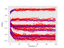
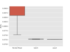
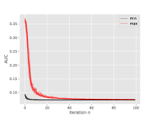
Figure 2: Pima dataset. Left: running mean as a function of iteration $n$ for the exact (blue) and batch (red) algorithms ($10$ runs). Center: box-plot of the estimated minimum AUC for the three algorithms considered. (The plot is zoomed in for better readability.) Right: min/max of $l$ across iterations $n$ (different lines correspond to different runs) for the exact algorithm.

In Fig. 2, centre panel, we compare the variability (over $10$ runs) of the output of the three algorithms considered. One can see that both the exact and batch variants of our algorithm provide much lower empirical risk than the naive approach based on Nelder-Mead. Finally, the right panel reports the smallest and largest values of $l(X_{n}^{i})$ at iteration $n$ for the exact algorithm.

We repeat this experiment for the Sonar dataset, which is more challenging since $p=60$. Results are displayed in Fig. 3. Here we do not report the output of the Nelder-Mead algorithm, as they were found to be off, with a median over 10 runs of 0.25, which is more than an order of magnitude higher than the output of the other two algorithms. We notice that a larger number of iterations is required to achieve convergence in this case, and both algorithms were run for 4000 iterations. Note however that in this case 20 iterations of the batch algorithm requires the same number of data accesses as a single iteration of the exact algorithm (i.e. $n^{+}n^{-}/n_{\mathrm{batch}}\approx 20$), so the batch algorithm remains a cheap and therefore appealing approach for AUC minimisation, in the present scenario.

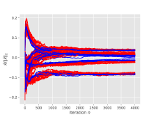
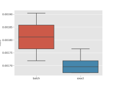
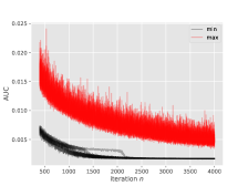
Figure 3: Same plots as Figure 2 for the Sonar dataset. For the left plot, only the last 5 components are shown. For the center plot, Nelder-Mead is excluded because results are far off. For the right plot, the first 300 iterations are not plotted to improve readibility.

Extensions

We finish this section with some remarks concerning more general implementations. The algorithm described in this section is a particular instance of sequential Monte Carlo (SMC) samplers Del Moral et al., (2006), where the aim is to sample from a sequence of probability distributions sequentially in time. Here we took advantage of the fact that sampling from $\pi_{\theta,\gamma}$ is routine and in fact used an SMC adaptive strategy to adapt $\lambda$. In more complex scenarios this may not be possible and instead one may choose to propagate samples with a more general mutation kernel, typically resulting in a perturbation of samples from previous generation, which is then corrected with an importance weight. Another advantage is that good particles can be recycled from one generation to the next and not resampled anew. Further extensions could involve the inclusion of persistency of movement in a particular direction i.e. take advantage of regularity of variations of $l(\cdot)$ e.g. “in the tails”, in the same way gradient information allows fast algorithms.

3 Results on gradient descent with smooth approximations

In this section we review essential notions and tools required to address the minimisation of a function $f:\mathbb{R}^{d}\to\mathbb{R}$, assumed lower-bounded, not necessarily differentiable, but for which there exists a sequence of differentiable approximations $\left\{f_{n}:\mathbb{R}^{d}\to\mathbb{R},\ f_{n}\in C^{1}(\mathbb{R}^{d}),\ n\in\mathbb{N}\right\}$, convergent to $f$ in a sense to be made precise below. In this scenario it is natural to suggest the non-homogeneous gradient descent algorithm

$$\theta_{n+1}=\theta_{n}-\gamma_{n}\nabla f_{n}(\theta_{n})\,,$$ (5)

where $\left\{\gamma_{n}\in\mathbb{R}_{+},\ n\in\mathbb{N}\right\}$ with $\gamma_{n}\downarrow 0$, in the hope that tracking the sequence points in $\left\{\operatorname*{argmin}f_{n},n\in\mathbb{N}\right\}$ will lead us to minima of $f$. This is however a subtle matter. To start with, non-differentiable functions such as in Fig. 4(a) do not have a minimum as it is not lower-semicontinuous, a weak property ensuring the existence of minima. A more substantial issue is that even when perfect minimisation of $f_{n}$ for all $n\in\mathbb{N}$ is possible, the intuitive set-limit (properly defined in Def. C.4) $\lim_{n}\left\{\operatorname*{argmin}f_{n}\right\}=\operatorname*{argmin}f$ may not hold. This is illustrated in Figure 4(b) with a counterexample illustrating that even uniform convergence of $\left\{f_{n},n\in\mathbb{N}\right\}$ to $f$ is not sufficient to ensure $\lim_{n}\left\{\operatorname*{argmin}f_{n}\right\}=\operatorname*{argmin}f$. An important point in the present paper is that using smoothed approximations for minimisation may not work in certain contrived scenarios.

Example 3.1.

With the notation from Section 1, for $d=2$ consider the function $l(x):=\min\{1,|x_{1}|\}\mathbf{1}\{x_{1}=x_{2}\}+\mathbf{1}\{x_{1}\neq x_{2}\}$. This function is such that $\mathrm{Leb}\{x\in\mathbb{R}^{2}\colon l(x)<1\}=0$ and as a consequence for any $\theta\in\Theta$ and $\gamma>0$, $h_{\gamma}(\theta)=1$, that is the smoothed functions $\theta\mapsto h_{\gamma}(\theta)$ “cannot see the minimum” at zero. In general a requirement therefore seems to be that for any $x^{*}\in\arg\min_{x\in\mathsf{X}}l(x)$

$$\lim_{\gamma\downarrow 0}\gamma^{-d/2}\int\exp\big{(}-l(x)\big{)}\phi\Bigl{(}\frac{x-x^{*}}{\sqrt{\gamma}}\Bigr{)}{\mathrm{d}}x=\exp\big{(}-l(x^{*})\big{)}\,.$$ (6)

In the toy countexample the left hand side is equal to $\exp(-1)$ while the right hand side is equal to $1$. The condition precludes the existence of sets $A\ni x^{*}$ such that for some $c>0$ for all $x\in A$ we have $l(x)\geq l(x^{*})+c$ and $\int_{A}\pi_{x^{*},\gamma}(x){\mathrm{d}}x\rightarrow_{\gamma\downarrow 0}1$.

Epi-convergence of $\left\{f_{n}:\mathbb{R}^{d}\to\mathbb{R},\ n\in\mathbb{N}\right\}$ to $f$ is a suitable and flexible form of convergence ensuring that smoothing techniques combined with exact optimisation achieve their goal. Ensuring this property is a natural prerequisite to the justification of the recursion (5) to optimise $f$. However it must be noted that convergence in this framework differs from what is usually understood as convergence; weaker forms of the set limit $\lim_{n}\left\{\operatorname*{argmin}f_{n}\right\}=\operatorname*{argmin}f$ can be obtained, depending on the strength of the assumptions. The following result, due to (Ermoliev et al., , 1995, Theorem 4.7), exemplifies what one may hope to be able to deduce. Assume that $\left\{f_{n}:\mathbb{R}^{d}\to\mathbb{R},\ f_{n}\in C^{1}(\mathbb{R}^{d}),\ n\in\mathbb{N}\right\}$ epi-converges (properly defined in Def. 3.4) to $f$, then

$$\theta_{\infty}\in\mathbb{R}^{d}\ \text{local minimum of }f\ \Rightarrow\ \exists\left\{\theta_{n},\ n\in\mathbb{N}\right\}\ \text{s.t.}\ \theta_{n}\to\theta_{\infty}\ \text{and}\ ||\nabla f_{n}(\theta_{n})||\to 0\,.$$ (7)

The practical implication of this result is that if a sequence $\left\{\theta_{n}\in\mathbb{R}^{d},\ n\in\mathbb{N}\right\}$ admits a subsequence $\left\{\theta_{n_{k}}\in\mathbb{R}^{d},\ k\in\mathbb{N}\right\}$ convergent to some $\theta_{\infty}\in\mathbb{R}^{d}$ and such that $\lim_{k}||\nabla f_{n_{k}}(\theta_{n_{k}})||=0$, then $\theta_{\infty}$ is a valid candidate as a local minimum of $f$, and accumulations points not satisfying the latter condition must be rejected. Theorem 3.2 in this manuscript presents an adaptation to our setting of Ermoliev et al., (1995) result.

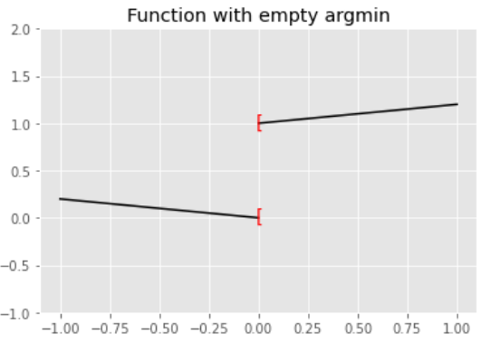
(a)

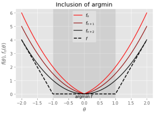
(b)

Figure 4: Left: example of a function with empty $\operatorname*{argmin}$. Right: A sequence of functions $\left\{f_{n},\ n\in\mathbb{N}\right\}$ (red-to-black color palette) that epi-converges to the function $f$. The picture is inspired by (Rockafellar and Wets, , 1998, Figure 7.7). It is clear that here $\operatorname*{argmin}f_{n}\subset\operatorname*{argmin}f$.

3.1 Lower-semi continuity

The notion of $\liminf$ for functions $f:\mathbb{R}^{d}\to\mathbb{R}$, frequently used in the manuscript, is defined as follows.

Definition 3.1.

Let $f:\mathbb{R}^{d}\to\mathbb{R}$. For $\theta_{0}\in\mathbb{R}^{d}$,

$$\liminf_{\theta\to\theta_{0}}f(\theta):=\sup_{\epsilon>0}\left(\inf\left\{f(\theta);\ \theta\in\mathbb{B}(\theta_{0},\epsilon)\right\}\right)$$

where $\mathbb{B}(\theta_{0},\epsilon)$ denotes a closed metric ball with center $\theta_{0}$ and radius $\epsilon>0$.

Definition 3.2 (Lower semicontinuity).

(Rockafellar and Wets, , 1998, Def. 1.5) A function $f:\mathbb{R}^{d}\to\mathbb{R}$ is said to be

1. lower-semicontinous ($\mathrm{lsc}$) at $\theta_{0}\in\mathbb{R}^{d}$ if

   $$\liminf_{\theta\to\theta_{0}}f(\theta)\geq f(\theta_{0})$$ (8)

2. lower-semicontinous if the above holds for any $\theta_{0}\in\mathbb{R}^{d}$.

Remark 3.1.

For $\theta_{0}\in\mathbb{R}^{d}$ and $\epsilon>0$, $\inf\left\{f(\theta);\ \theta\in\mathbb{B}(\theta_{0},\epsilon)\right\}\leq f(\theta_{0})$, therefore, $\liminf_{\theta\to\theta_{0}}f(\theta)\leq f(\theta_{0})$; hence condition (8) is equivalent to $\liminf_{\theta\to\theta_{0}}f(\theta)=f(\theta_{0})$.

By definition, any lower-semicontinuous, lower-bounded function has a minimum on $\mathbb{R}^{d}$.

Definition 3.3 (Strong lower semicontinuity).

A function $f:\mathbb{R}^{d}\to\mathbb{R}$ is said to be

1. strongly lower-semicontinous ($slsc$) at $\theta\in\mathbb{R}^{d}$ if it is lower semicontinous at $\theta\in\mathbb{R}^{d}$ and there exists a sequence $\left\{\theta_{n},\ n\in\mathbb{N}\right\}$, $\theta_{n}\to\theta$ such that $f(\theta_{n})\to f(\theta)$.

2. strongly lower-semicontinuous if the above holds for any $\theta\in\mathbb{R}^{d}$.

In words, strong lower-semicontinuity is lower-semicontinuity excluding discontinuities at isolated points. Remark that we do not make any assumption on smoothness of the function; the class of strongly lower-semicontinuous functions includes indicator functions of closed sets, step functions, ceiling functions; but also not-everywhere differentiable continuous and discontinuous (if there are not isolated discontinuity points) functions.

Example 3.2.

The step function $f:\mathbb{R}\to\mathbb{R}$ defined by

$$f(\theta)=\begin{cases}1,\ \theta>0\\ 0,\ \theta\leq 0\end{cases}\,.$$

is strongly lower-semicontinuous. The following function is lower-semicontinuous everywhere but at $\theta=0$,

$$f(\theta)=\begin{cases}1,\ \theta\geq 0\\ 0,\ \theta<0\end{cases}\,.$$

Intuitively, we can note that the part of the space above the graph of this function, commonly called epigraph of $f$, is not a closed set, which in fact precludes lower-semicontinuity: see Appendix C.1 for more results on lower-semicontinuity and epigraphs.

Example 3.3.

Consider a function $f:\mathbb{R}^{d}\to\mathbb{R}$. The epigraphical closure of $f$, denoted $\mathrm{cl_{e}}$,

$$\mathrm{cl_{e}}\ f(\theta):=\liminf_{\theta^{\prime}\to\theta}f(\theta^{\prime})\,,\ \theta\in\mathbb{R}^{d}$$

is lower-semicontinuous, with $\mathrm{cl_{e}}f(\theta)\leq f(\theta)$. More details can be found in (Rockafellar and Wets, , 1998, Chapter 1, Section D).

Example 3.4 (Probability functions).

Let $P$ be a distribution on $\mathcal{U}$ and let $U\sim P$ random variable, and let $g:\mathbb{R}\times\mathcal{U}\to\mathbb{R}$ be a two-variable function such that the objective

$$f(\theta)=-\int_{\mathcal{U}}\mathbf{1}\left\{g(\theta,u)<0\right\}P(\mathrm{d}u)$$

has a minimum on $\mathbb{R}$. As the function $\mathbf{1}\left\{\cdot\right\}$ is discontinuous, $f$ will in general not be everywhere differentiable (and hence non-smooth). For example, if $g(\theta,u)=\theta+u$ and $P$ is chosen to be the uniform $\mathrm{Unif}\left[0,1\right]$, we have

$$L(\theta)=\begin{cases}|\theta|-1,|\theta|\leq 1\\ 0,\ \ \ \ \ \ \ \ |\theta|>1\end{cases}\,.$$

which is nonsmooth at $\theta\in\left\{0,1,-1\right\}$. This type of objective functions is for instance considered in Norkin, (1993).

3.2 Epi-convergence and convergence in minimisation

As discussed in the introduction of this section, epi-convergence is the right notion of convergence for $\left\{f_{n}:\mathbb{R}^{d}\to\mathbb{R},\ n\in\mathbb{N}\right\}$ to $f$ to formulate and establish convergence of the type of recursion (5). We therefore start with some definitions – a more classical abstract definition in terms of epigraphs convergence is provided in Appendix C.3.

Definition 3.4 (Epi-convergence).

A sequence of functions $\left\{f_{n}:\mathbb{R}^{d}\to\mathbb{R},\ n\in\mathbb{N}\right\}$ epi-converges to a function $f:\mathbb{R}^{d}\to\mathbb{R}$ if for each $\theta\in\mathbb{R}^{d}$

1. $\liminf_{n}f_{n}(\theta_{n})\geq f(\theta)$ for any sequence $\theta_{n}\to\theta$

2. $\lim_{n}f_{n}(\theta_{n})=f(\theta)$ for some sequence $\theta_{n}\to\theta$.

Thus, we say that $f$ is the epi-limit of $\left\{f_{n},\ n\in\mathbb{N}\right\}$.

We can immediately note that if a function $f:\mathbb{R}^{d}\to\mathbb{R}$ is the epi-limit of some sequence $\left\{f_{n},\ n\in\mathbb{N}\right\}$, then $f$ is necessarily lower-semicontinuous.

Example 3.5.

The three examples below aim to illustrate how epi-convergence differs from standard functional limits. Consider $\left\{f_{n}\colon\mathbb{R}\rightarrow\mathbb{R},\ n\in\mathbb{N}\right\}$ where,

1. $f_{n}(\theta):=-e^{-n\theta^{2}}$, then the sequence epi-converges to

   $$f(\theta):=\begin{cases}-1,\ \theta=0\\ 0,\ \ \ \ \theta\neq 0\,.\end{cases}$$

   In fact, it converges pointwise to the same limit. However, epi-convergence generally differs from e.g. pointwise convergence, as the following example shows.

2. $f_{n}(\theta)=e^{-n\theta^{2}}$, then the sequence epi-converges to $f\equiv 0$, as in particular $\lim_{n}f_{n}(n^{-\alpha})=0$ for $\alpha\in(0,1/2)$; we see here how epi-convergence differs from e.g. pointwise convergence since $\lim f_{n}(0)=1$ here,

3. $f_{n}(\theta)=(-1)^{n}e^{-n\theta^{2}}$, then fhe sequence fails to epi-converge as for $\theta=0$ and any sequence $\left\{\theta_{n},\ n\in\mathbb{N}\right\}$ such that $\theta_{n}\to 0$ we have $\lim_{n}(-1)^{n}f_{n}(\theta_{n})=1$, and therefore $\lim_{n}f_{n}(\theta_{n})$ does not exist.

Epi-convergence is concerned with the set convergence of epigraphs, that is, of the part of the space above the graph of the functions; again full details are provided Appendix C for more details, but not required to understand the nature of our convergence results.

The following Theorem highlights two main consequences of epi-convergence, describing what type of results one can expect about convergence of minima and infima. Below, we say that a function $g:\mathbb{R}^{d}\to\mathbb{R}$ is eventually level-bounded if for each $a\in\mathbb{R}^{d}$ the sequence of level-sets $\left\{\mathrm{lev}_{\leq a}f_{n},\ n\in\mathbb{N}\right\}$ is eventually bounded. For instance, a sequence of eventually lower-bounded functions is eventually level-bounded.

Theorem 3.1 (Rockafellar and Wets, (1998), Theorem 7.33).

Let

1. $f:\mathbb{R}^{d}\to\mathbb{R}$ be a lower-bounded, lower-semicontinuous function,

2. $\left\{f_{n}:\mathbb{R}^{d}\to\mathbb{R},\ n\in\mathbb{N}\right\}$ be a sequence of lower-semicontinuous functions such that

   1. $\left\{f_{n},\ n\in\mathbb{N}\right\}$ epi-converges to $f$,

   2. $\left\{f_{n},\ n\in\mathbb{N}\right\}$ is eventually level-bounded.

Then,

1. $\underset{\theta\in\mathbb{R}^{d}}{\inf}f_{n}(\theta)\to\underset{\theta\in\mathbb{R}^{d}}{\inf}f(\theta)$,

2. $\mathrm{Limsup}_{n}\operatorname*{argmin}f_{n}\subset\operatorname*{argmin}f$.

In (Rockafellar and Wets, , 1998, Chapter 5) it is remarked that looking for the inclusion $\mathrm{Limsup}_{n}\ \operatorname*{argmin}f_{n}\subset\operatorname*{argmin}f$ should be preferred over the stronger result $\lim_{n}\left\{\operatorname*{argmin}f_{n}\right\}=\operatorname*{argmin}f$. Figure 4(b) provides an example of a sequence of functions that epi-converge (in fact, they converge uniformly) to a function $f$, and where it is not true that every point of $\operatorname*{argmin}f$ is in the limit of $\operatorname*{argmin}f_{n}$. Note that, however, any $\theta\in\operatorname*{argmin}f$ in the figure can be expressed as a limit of points $\theta_{n}$ that are $\epsilon_{n}$-optimal for $f_{n}$ in the sense of equation (36), for $\epsilon_{n}\downarrow 0$.

We now turn to results characterising local minima $\theta_{*}$ of $f$ as accumulation points of sequences $\left\{\theta_{n}\in\mathbb{R}^{d},n\in\mathbb{N}\right\}$ in the situation where an epi-convergent and differentiable approximating sequence $\left\{f_{n}:\mathbb{R}^{d}\to\mathbb{R},\ n\in\mathbb{N}\right\}$ exists. In particular the existence of $\theta_{n}\rightarrow\theta_{*}$ is established, for which $\lim_{n}\|\nabla f_{n}(\theta_{n})\|=0$. As a consequence for any algorithm producing a sequence $\left\{\theta_{n}\in\mathbb{R}^{d},n\in\mathbb{N}\right\}$ from which a convergent sequence $\theta_{n_{k}}\rightarrow\theta_{*}\in\mathbb{R}^{d}$ can be extracted, then if $\lim_{n_{k}}\|\nabla f_{n_{k}}(\theta_{n_{k}})\|\neq 0$ we reject $\theta_{*}$ as a local minimum.

We begin with two Lemmata that allow us to prove the key result of this section. The following Lemma describes a key differentiability property of the convolution of two functions, one of which is of class $C^{1}(\mathbb{R}^{d})$.

Lemma 3.1 (Rockafellar and Wets, (1998), Theorem 9.67).

Let $f,g:\mathbb{R}^{d}\to\mathbb{R}$ be locally integrable and assume that $g\in C^{1}(\mathbb{R}^{d})$. Then the function $\theta\mapsto\int f(u)g(\theta-u)\mathrm{d}u$ belongs to $C^{1}(\mathbb{R}^{d})$ with

$$\nabla\int f(u)g(\theta-u)\mathrm{d}u=\int f(u)\nabla g(\theta-u)\mathrm{d}u,\ \ \theta\in\mathbb{R}^{d}.$$

The lemma below describes an important property of convergent sequences that attain $\epsilon$-optimal points of epi-convergent functions.

Lemma 3.2 (Attouch, (1984), Theorem 1.10).

Let $D\subseteq\mathbb{R}^{d}$ and

1. $\left\{f_{n}:\mathbb{R}^{d}\to\mathbb{R},\ n\in\mathbb{N}\right\}$ be epi-convergent to $f:\mathbb{R}^{d}\to\mathbb{R}$ for all $\theta\in D$

2. $\left\{\theta_{n}\in\mathbb{R}^{d},\ n\in\mathbb{N}\right\}$ be such that $\theta_{n}\to\theta_{*}\in D$ and for $\left\{\epsilon_{n}\in\mathbb{R}_{+},n\in\mathbb{N}\right\}$ with $\epsilon_{n}\downarrow 0$

   $$f_{n}(\theta_{n})\leq\underset{\theta\in D}{\inf}f_{n}(\theta)+\epsilon_{n},\ n\in\mathbb{N}\,.$$

Then, $\theta_{*}\in\underset{\theta\in D}{\operatorname*{argmin}}\ f$.

Finally, the following justifies an optimisation procedure for finding local minima of $l$ by tracking minimisers of differentiable functions $\left\{h_{n},\ n\in\mathbb{N}\right\}$ that epi-converge to $l$. The proof of the result is a generalisation of the proof of (Ermoliev et al., , 1995, Theorem 4.7). While in the latter paper the result is stated for a strongly lower-semicontinuous $f$ and auxiliary mollifiers with bounded support (implying epi-convergence in their setting), we noted that it is enough for $f$ to be lower-semicontinuous and for the auxiliary mollifiers to be Gaussian if epi-convergence is put as an assumption of the theorem. This extends its validity and widens the class of methods whose convergence can be proven in terms of the Theorem below.

Theorem 3.2.

Let,

1. $f:\mathbb{R}^{d}\to\mathbb{R}$ be locally integrable, lower bounded and lower-semicontinuous,

2. $\left\{f_{n}:\mathbb{R}^{d}\to\mathbb{R},\ n\in\mathbb{N}\right\}$ be a sequence of differentiable functions epi-convergent to $f$.

Then for any $\theta_{*}\in\mathrm{loc-}\operatorname*{argmin}f$ there exists $\left\{\theta_{k}\in\mathbb{R}^{d},\ k\in\mathbb{N}\right\}$ such that $\theta_{k}\to\theta_{*}$ and $\lim_{k}||\nabla f_{k}(\theta_{k})||=0$.

Proof.

Let $\theta_{*}$ be a local minimiser of $f$, define $\phi(\theta):=f(\theta)+||\theta-\theta_{*}||^{2}$ and let $V$ be a sufficiently small compact set such that $\theta_{*}\in V$ and $\operatorname*{argmin}_{\theta\in V}\ \phi(\theta)=\left\{\theta_{*}\right\}$ - that is, $\theta_{*}$ is the unique global minimiser of $\phi$ on $V$. The uniqueness of the minimiser on $V$, ensured by the auxiliary function $\phi$, excludes potential issues arising from working with a locally flat function, and more generally guarantees that a (sub-) sequence converging to $\theta_{*}$ as per Lemma 3.2 exists, as we are going to illustrate. Consider the sequence of mollifiers $\left\{\psi_{n}:\mathbb{R}^{d}\to\mathbb{R}_{+},\ n\in\mathbb{N}\right\}$ with

$$\psi_{n}(z):=(2\pi\gamma_{n})^{-d/2}\exp\left\{-\frac{||z||^{2}}{2\gamma_{n}}\right\}$$

and $\left\{\gamma_{n}\in\mathbb{R}_{+},n\in\mathbb{N}\right\}$ such that $\gamma_{n}\downarrow 0$. From (Ermoliev et al., , 1995, Remark 3.14) we have $\psi_{n}\in C^{1}(\mathbb{R}^{d}),\ \ \int\psi_{n}(z)\mathrm{d}z=1$, $n\in\mathbb{N}$, and for every $\delta>0$,

$$\lim_{n}\int_{\left\{||z||>\delta\right\}}\psi_{n}(z)\mathrm{d}z=0,\ \text{and}\ \lim_{n}\int_{||z||>\delta}||z+\theta-\theta_{*}||^{2}\psi_{n}(z)\mathrm{d}z=0$$

uniformly in $\theta\in\mathbb{R}^{d}$.
Let $\beta_{n}(\theta,\theta_{*}):=\int||z+\theta-\theta_{*}||^{2}\psi_{n}(z)\mathrm{d}z$, $n\in\mathbb{N},\ \theta\in V$, and define the auxiliary functions

$$\phi_{n}(\theta):=f_{n}(\theta)+\beta_{n}(\theta,\theta_{*}),\ n\in\mathbb{N},\ \theta\in V.$$

Note that

• the functions $\left\{\beta_{n},\ n\in\mathbb{N}\right\}$ are of class $C^{1}(\mathbb{R}^{d})$ by Lemma 3.1,

• For the above mollifiers, $\left\{\beta_{n},\ n\in\mathbb{N}\right\}$ epi-converge to $\theta\mapsto||\theta-\theta_{*}||^{2}$ on $V$ due to (Ermoliev et al., , 1995, Theorem 3.7 and Remark 3.14) – in fact, they converge uniformly,

• By assumption, $\left\{f_{n},\ n\in\mathbb{N}\right\}$ is a sequence of differentiable functions that epi-converge to $f$; therefore, $\left\{\phi_{n},\ n\in\mathbb{N}\right\}$ is a sequence of well-defined differentiable (hence continuous) functions on $V$ that epi-converge to $\phi$ on $V$.

Let $\left\{\bar{\theta}_{n}\in V,\ n\in\mathbb{N}\right\}$ be a sequence of minimisers of $\left\{\phi_{n},\ n\in\mathbb{N}\right\}$, which exists since for any $n\in\mathbb{N}$, $\phi_{n}$ is continuous and $V$ a compact set. From the compactness of $V$ there exists a convergent subsequence $\left\{\theta_{n}\in V,\ n\in\mathbb{N}\right\}$ of $\left\{\bar{\theta}_{n}\in V,\ n\in\mathbb{N}\right\}$. By Lemma 3.2, it holds that $\theta_{n}\to\theta_{*}$. We now turn to the second statement. For each $n\in\mathbb{N}$,

$$0=\nabla\phi_{n}(\theta_{n})=\nabla f_{n}(\theta_{n})+\nabla\beta_{n}(\theta_{n},\theta_{*}).$$ (9)

and in the limit,

$$\lim_{n}\nabla f_{n}(\theta_{n})=-\lim_{n}\nabla\beta_{n}(\theta_{n},\theta_{*})=0.$$ (10)

which proves the statement.
In order to show the last equality, by continuity of the function $\theta\mapsto||\theta||^{2}$ one can use Lemma 3.1 and write, for every $k$,

$$\nabla\beta_{k}(\theta_{k},\theta_{*}) =\nabla\int||z+\theta_{k}-\theta_{*}||^{2}\psi_{k}(z)\mathrm{d}z$$

$$\overset{\text{Lemma \ref{lemma: differentiability of averages}}}{=}\int\nabla||z+\theta_{k}-\theta_{*}||^{2}\psi_{k}(z)\mathrm{d}z$$

$$=\int 2(z+\theta_{k}-\theta_{*})\psi_{k}(z)\mathrm{d}z$$

$$=2\left\{\int z\psi_{k}(z)\mathrm{d}z+\theta_{k}-\theta_{*}\right\}.$$

We can now note that, by assumption, $\int z\psi_{k}(z)\mathrm{d}z=0$ for every $k\in\mathbb{N}$; moreover, $\theta_{k}\to\theta_{*}$. Therefore, the last equality in (10) holds. ∎

3.3 Stability and convergence of time-inhomogeneous gradient descent

The following result establishes convergence of time inhomogeneous gradient algorithms to local minima of $l(\cdot)$. This generalizes results such as Gupal and Norkin, (1977), not requiring confinement of the sequence $\{\theta_{n},n\in\mathbb{N}\}$ for example. The result is specialised to exploit the fact that for any $n\in\mathbb{N}$ the map $\theta\mapsto\|\nabla f_{n}(\theta)\|$ is uniformly bounded in $\theta\in\Theta$.

Theorem 3.3.

For differentiable functions $\{f_{n}\colon\mathbb{R}^{d}\rightarrow\mathbb{R},\ n\in\mathbb{N}\}$ and $\{\gamma_{n}\in\mathbb{R}_{+},\ n\in\mathbb{N}\}$ consider the recursion defined for some $\theta_{0}\in\mathbb{R}^{d}$ and for $n\geq 0$

$$\theta_{n+1}=\theta_{n}-\gamma_{n}\nabla f_{n}(\theta_{n})\,.$$ (11)

Let $\alpha\in[0,2]$ and $\{L_{n}\in\mathbb{R}_{+},\ n\in\mathbb{N}\}$ and $\{\delta_{n}\in[0,\infty),\ n\in\mathbb{N}\}$ be such that

$$\limsup_{n\rightarrow\infty}\gamma_{n}L_{n}<1,\quad\lim_{n\rightarrow\infty}(\delta_{n}/\gamma_{n})=\lim_{n\rightarrow\infty}(\delta_{n}/\gamma_{n+1})=0,\quad\sum_{n=1}^{\infty}\gamma_{n}=\infty.$$

Assume that the following conditions hold:

1. $\inf_{(n,\theta)\in\mathbb{N}\times\mathbb{R}^{d}}f_{n}(\theta)>-\infty$.

2. for all $\theta,\theta^{\prime}\in\mathbb{R}^{d}$ and $n\in\mathbb{N}$,

   $$f_{n}(\theta^{\prime})\leq f_{n}(\theta)+\langle\nabla f_{n}(\theta),\theta^{\prime}-\theta\rangle+L_{n}\|\theta^{\prime}-\theta\|^{2}.$$

3. for all $\theta\in\mathbb{R}^{d}$ and $n\in\mathbb{N}$,

   $$f_{n+1}(\theta)-f_{n}(\theta)\leq\delta_{n}\big{[}1+\|\nabla f_{n+1}(\theta)\|^{\alpha}\big{]}.$$

4. either of the following conditions holds (with the convention $0\cdot\infty=0$):

   1. Condition 3 holds with $\alpha=0$.

   2. $$\lim_{n\rightarrow\infty}\frac{\delta_{n}\sup_{\theta\in\mathbb{R}^{d}}\|f_{n+1}(\theta)\|^{\alpha/2}}{\gamma_{n+1}^{\alpha/2}\sum_{m=1}^{n}\gamma_{m}}=0$$

   3. $$\lim_{n\rightarrow\infty}\frac{\delta_{n}\sup_{\theta\in\mathbb{R}^{d}}\|\nabla f_{n+1}(\theta)\|^{\alpha}}{\sum_{m=1}^{n}\gamma_{m}}=0$$

   4. there exists a constant $\beta\in(0,1]$ and a sequence $\{\tilde{L}_{n}\in(0,\infty)\colon n\geq 1\}$ such that, for all $\theta,\theta^{\prime}\in\mathbb{R}^{d}$ and $n\in\mathbb{N}$, $|f_{n}(\theta)-f_{n}(\theta^{\prime})|\leq\tilde{L}_{n}\|\theta-\theta^{\prime}\|^{\beta}$ and such that

      $$\lim_{n\rightarrow\infty}\frac{\delta_{n}\tilde{L}_{n+1}^{\frac{\alpha}{2-\beta}}}{\gamma_{n+1}^{\alpha(1-\beta)/(2-\beta)}\sum_{m=1}^{n}\gamma_{m}}=0.$$

Then, there exists a subsequence $\left\{\theta_{n_{k}},\ k\in\mathbb{N}\right\}$ of $\{\theta_{n},n\geq 1\}$ such that $\lim_{k\rightarrow\infty}\|\nabla f_{n_{k}}(\theta_{n_{k}})\|=0$.

Proof.

Under 2 and using (11), for all $n\geq 1$ we have

$$\begin{split}f_{n}(\theta_{n+1})&\leq f_{n}(\theta_{n})+\langle\nabla f_{n}(\theta_{n}),\theta_{n+1}-\theta_{n}\rangle+L_{n}\|\theta_{n+1}-\theta_{n}\|^{2}\\ &=f_{n}(\theta_{n})-\gamma_{n}\|\nabla f_{n}(\theta_{n})\|^{2}\big{(}1-L_{n}\gamma_{n}\big{)}\end{split}$$ (12)

Let $n_{1}\in\mathbb{N}$ and $\epsilon_{1}\in(0,1)$ be such that $1-\gamma_{n}L_{n}\geq\epsilon_{1}$ for all $n\geq n_{1}$. Then, for all $n\geq n_{1}$ we have, using (12) and under 3,

$$\begin{split}f_{n+1}(\theta_{n+1})&\leq f_{n}(\theta_{n})-\gamma_{n}\|\nabla f_{n}(\theta_{n})\|^{2}\big{(}1-L_{n}\gamma_{n}\big{)}+f_{n+1}(\theta_{n+1})-f_{n}(\theta_{n+1})\\ &\leq f_{n}(\theta_{n})-\gamma_{n}\epsilon_{1}\|\nabla f_{n}(\theta_{n})\|^{2}+\delta_{n}\big{(}1+\|\nabla f_{n+1}(\theta_{n+1})\|^{\alpha}\big{)}.\end{split}$$ (13)

We now prove the result of the theorem by contradiction. To this aim, assume that there exists an $\epsilon_{2}\in(0,1)$ and an $n_{2}\in\mathbb{N}$ such that $\|\nabla f_{n}(\theta_{n})\|\geq\epsilon_{2}$ for all $n\geq n_{2}$.

Then, for all $n\geq n_{3}:=\max\{n_{1},n_{2}\}$ we have, by (13) and letting $\epsilon_{3}=\epsilon_{1}\epsilon_{2}^{2-\alpha}$

$$f_{n+1}(\theta_{n+1}) \leq f_{n}(\theta_{n})-\epsilon_{3}\gamma_{n}\|\nabla f_{n}(\theta_{n})\|^{\alpha}+\delta_{n}\big{(}1+\|\nabla f_{n+1}(\theta_{n+1})\|^{\alpha}\big{)}.$$

and thus, for all $n\geq n_{3}$, we have

$$\begin{split}f_{n+1}(\theta_{n+1})&\leq f_{n_{3}}(\theta_{n_{3}})-\epsilon_{3}\sum_{m=n_{3}}^{n}\gamma_{m}\|\nabla f_{m}(\theta_{m})\|^{\alpha}\\ &\hskip 71.13188pt+\bigg{(}\sum_{m=n_{3}}^{n}\delta_{m}\|\nabla f_{m+1}(\theta_{m+1})\|^{\alpha}\bigg{)}+\sum_{m=n_{3}}^{n}\delta_{m}\\ &\leq f_{n_{3}}(\theta_{n_{3}})-\sum_{m=n_{3}+1}^{n}\|\nabla f_{m}(\theta_{m})\|^{\alpha}\big{(}\epsilon_{3}\gamma_{m}-\delta_{m-1}\big{)}\\ &\hskip 71.13188pt+\delta_{n}\|\nabla f_{n+1}(\theta_{n+1})\|^{\alpha}+\sum_{m=n_{3}}^{n}\delta_{m}\,.\end{split}$$ (14)

To proceed further assume without loss of generality that $n_{3}$ is sufficiently large so that, for some $\epsilon_{4}\in(0,1)$, we have $\epsilon_{3}\gamma_{n}-\delta_{n-1}\geq\epsilon_{4}\gamma_{n}$ for all $n\geq n_{3}$. Then, using (14), for all $n\geq n_{3}$ we have

$$\begin{split}f_{n+1}(\theta_{n+1})&\leq f_{n_{3}}(\theta_{n_{3}})-\epsilon_{4}\epsilon_{2}^{\alpha}\Big{(}\sum_{m=n_{3}+1}^{n}\gamma_{m}\Big{)}+\delta_{n}\|\nabla f_{n+1}(\theta_{n+1})\|^{\alpha}+\sum_{m=n_{3}}^{n}\delta_{m}\\ &=f_{n_{3}}(\theta_{n_{3}})-\sum_{m=n_{3}+1}^{n}\gamma_{m}\bigg{(}\epsilon_{4}\epsilon_{2}^{\alpha}-\frac{\delta_{n}\|\nabla f_{n+1}(\theta_{n+1})\|^{\alpha}}{\sum_{m=n_{3}+1}^{n}\gamma_{m}}-\frac{\sum_{m=n_{3}}^{n}\delta_{m}}{\sum_{m=n_{3}+1}^{n}\gamma_{m}}\bigg{)}\end{split}$$ (15)

where, under the assumptions of the theorem,

$$\lim_{n\rightarrow\infty}\frac{\sum_{m=n_{3}}^{n}\delta_{m}}{\sum_{m=n_{3}+1}^{n}\gamma_{m}}=0,\quad\lim_{n\rightarrow\infty}\sum_{m=n_{3}+1}^{n}\gamma_{m}=\infty.$$

Therefore, if

$$\lim_{n\rightarrow\infty}\frac{\delta_{n}\|\nabla f_{n+1}(\theta_{n+1})\|^{\alpha}}{\sum_{m=n_{3}+1}^{n}\gamma_{m}}=0$$ (16)

then, by (15), we have $\lim_{n\rightarrow\infty}f_{n+1}(\theta_{n+1})=-\infty$ which contradicts 1. Hence, to complete the proof it remains to show that (16) holds under the assumption of the theorem.

Remark first that (16) trivially holds under 4a and under 4c. Next, remark that, by (12), for all $n\geq n_{3}$ we have

$$f_{n}(\theta_{n+1})\leq f_{n}(\theta_{n})-\gamma_{n}\epsilon_{1}\|\nabla f_{n}(\theta_{n})\|^{2}\Leftrightarrow\|\nabla f_{n}(\theta_{n})\|^{\alpha}\leq\bigg{(}\frac{f_{n}(\theta_{n})-f_{n}(\theta_{n+1})}{\gamma_{n}\epsilon_{1}}\bigg{)}^{\frac{\alpha}{2}}$$ (17)

from which we readily obtain that (16) holds under 4b.

Finally, by (17), for all $n\geq n_{3}$ we have, under 4d and using (11),

$$\|\nabla f_{n}(\theta_{n})\|^{\alpha} \leq\bigg{(}\frac{\tilde{L}_{n}\|\theta_{n}-\theta_{n+1}\|^{\beta})}{\gamma_{n}\epsilon_{1}}\bigg{)}^{\frac{\alpha}{2}}=\bigg{(}\frac{\tilde{L}_{n}\gamma_{n}^{\beta}\|\nabla f_{n}(\theta_{n})\|^{\beta}}{\gamma_{n}\epsilon_{1}}\bigg{)}^{\frac{\alpha}{2}}$$

$$\Leftrightarrow$$

$$\|\nabla f_{n}(\theta_{n})\|^{\alpha(1-\beta/2)}\leq\bigg{(}\frac{\tilde{L}_{n}}{\gamma^{1-\beta}_{n}\epsilon_{1}}\bigg{)}^{\frac{\alpha}{2}}\Leftrightarrow\|\nabla f_{n}(\theta_{n})\|^{\alpha}\leq\bigg{(}\frac{\tilde{L}_{n}}{\gamma^{1-\beta}_{n}\epsilon_{1}}\bigg{)}^{\frac{\alpha}{2-\beta}}$$

and thus (16) follows. The proof of the theorem is complete. ∎

4 Convergence of Alg. 1: deterministic scenario

In this section we show that the results of Subsections 3.2 and 3.3 apply to Alg. 1 in the scenario where $\pi_{\theta,\gamma}$ is a Gaussian kernel as first introduced in the introduction, Section 1 – some of the intermediate results apply to approximations of the identity, but extension to the general EDM scenario is left for future work. Given an objective function $l:\mathbb{R}^{d}\to\mathbb{R}$, assumed lower bounded and strongly lower-semi-continuous, we essentially aim to establish epi-convergence to $l(\cdot)$ of the sequence of Laplace functionals $\left\{h_{n}:\mathbb{R}^{d}\to\mathbb{R},\ n\in\mathbb{N}\right\}$, defined, for an approximating sequence of the unity distribution $\left\{\psi_{n}\colon\mathbb{R}^{d}\rightarrow\mathbb{R}\right\},n\in\mathbb{N}$ (see Def. 4.1), by

$$h_{n}(\theta)=-\log\int e^{-l(x)}\psi_{n}(x-\theta)\mathrm{d}x,\quad\theta\in\mathbb{R}^{d}.$$ (18)

From this one can apply Theorem C.4 and Theorem 3.2 to characterise local minima. In addition we establish the conditions required for Theorem 3.3 to apply to this scenario.

4.1 Epi-convergence of Laplace functionals

It is useful for later calculations to note that by a change of variable $z=x-\theta$ we can equivalently write

$$h_{n}(\theta)=-\log\int e^{-l(\theta+z)}\psi_{n}(z)\mathrm{d}z.$$

We begin with the definition of mollifiers.

Definition 4.1 (mollifiers).

Let

$$\left\{\psi_{n}:\mathbb{R}^{d}\to\mathbb{R}_{+},\ \ \psi_{n}\in C^{1}(\mathbb{R}^{d}),\ \ \int\psi_{n}(z)\mathrm{d}z=1,\ n\geq 0\right\}$$

be a class of functions such that for every $\delta>0$,

$$\lim_{n}\int_{||z||>\delta}\psi_{n}(z)\mathrm{d}z=0.$$

We call such $\psi_{n}$ mollifiers.

Example 4.1 (Gaussian mollifiers).

Take $\psi_{n}(z)=\gamma_{n}^{-d/2}\phi\big{(}z\gamma_{n}^{-1/2}\big{)}$ with $\gamma_{n}\downarrow 0$, $n\in\mathbb{N}$, then $\left\{\psi_{n},\ n\in\mathbb{N}\right\}$ satisfy the definition of mollifiers.

The following theorem shows epi-convergence of Laplace functionals with mollifiers. The proof is inspired by ideas of (Ermoliev et al., , 1995, Theorems 3.2, 3.7 and Corollary 3.3) but extend their scope.

Theorem 4.1.

Let $l:\mathbb{R}^{d}\to\mathbb{R}$ be a lower-bounded, strongly lower-semicontinuous function. Let $\left\{\psi_{n}:\mathbb{R}^{d}\to\mathbb{R}_{+},\ n\in\mathbb{N}\right\}$ be mollifiers. Let $h_{n}(\theta)=-\log\int e^{-l(\theta+z)}\psi_{n}(z)\mathrm{d}z$, $\theta\in\mathbb{R}^{d}$, $n=1,2,\ldots$. Then, the sequence $\left\{h_{n}:\mathbb{R}^{d}\to\mathbb{R},\ n\in\mathbb{N}\right\}$ epi-converges to $l$.

Proof.

Fix $\theta\in\mathbb{R}^{d}$. We remark that by Proposition C.1, for a lower-bounded, integrable function $f:\mathbb{R}^{d}\to\mathbb{R}$, the epi-closure $\mathrm{cl_{e}}f$ is a lower-semicontinuous function and the hypo-closure $\mathrm{cl_{h}}f$ is an upper-semicontinuous function. Moreover, it holds $\mathrm{cl_{e}}f\leq f\leq\mathrm{cl_{h}}f$. Note also that if a function $f(\cdot)$ is lower-bounded and strongly lower-semicontinuous, then $e^{-f(\cdot)}$ is upper-bounded and strongly upper-semicontinuous. We break the proof into three steps.

• Define $g:=e^{-l}$ and $g_{n}(\cdot):=\int e^{-l(\cdot+z)}\psi_{n}(z)\mathrm{d}z$. Let $\theta_{n}\to\theta$. As first step, we show that

  $$\mathrm{cl_{e}}g(\theta)\leq\liminf_{n}g_{n}(\theta_{n})\leq\limsup_{n}g_{n}(\theta_{n})\leq\mathrm{cl_{h}}g(\theta)$$ (19)

  by only using that $l$ is lower-bounded and that $\left\{\psi_{n},\ n\in\mathbb{N}\right\}$ is a sequence of mollifiers.
  Fix $\epsilon>0$.

  • By upper-semicontinuity of $\mathrm{cl_{h}}e^{-l}$, there exists $\delta=\delta(\epsilon)>0$ such that

    $$\mathrm{cl_{h}}e^{-l(\theta+z)}\leq\mathrm{cl_{h}}e^{-l(\theta)}+\epsilon$$

    for all $z\in\mathbb{R}^{d}$ such that $||z||\leq\delta$.

  • For the above $\delta$, by definition of the mollifiers $\left\{\psi_{n},\ n\in\mathbb{N}\right\}$, we can choose $n=n(\epsilon,\delta)$ large enough such that, for all $n\geq n(\epsilon,\delta)$,

    $$0\leq\int_{||z||>\frac{\delta}{2}}e^{-l(\theta+z)}\psi_{n}(z)\mathrm{d}z\leq\underset{u\in\mathbb{R}^{d}}{\sup}e^{-l(u)}\int_{||z||\geq\frac{\delta}{2}}\psi_{n}(z)\mathrm{d}z\leq\frac{\epsilon}{2}.$$ (20)

  We first show the last inequality in equation (19). Let $\delta=\delta(\epsilon)$ as above. For all $n\geq n(\epsilon,\delta)$ large enough such that $||\theta_{n}-\theta||\leq\frac{\delta}{2}$, we have $||\theta_{n}-\theta+z||\leq\delta$ for any $z$ such that $||z||\leq\frac{\delta}{2}$. So we can write

  $$g_{n}(\theta_{n}) =\int e^{-l(\theta_{n}+z)}\psi_{n}(z)\mathrm{d}z$$

  $$=\int_{||z||\leq\frac{\delta}{2}}e^{-l(\theta_{n}+z)}\psi_{n}(z)\mathrm{d}z+\int_{||z||>\frac{\delta}{2}}e^{-l(\theta_{n}+z)}\psi_{n}(z)\mathrm{d}z$$

  $$\leq\int_{||z||\leq\frac{\delta}{2}}\mathrm{cl_{h}}e^{-l(\theta_{n}+z)}\psi_{n}(z)\mathrm{d}z+\frac{\epsilon}{2}$$

  $$=\int_{||z||\leq\frac{\delta}{2}}\mathrm{cl_{h}}e^{-l(\theta+\theta_{n}-\theta+z)}\psi_{n}(z)\mathrm{d}z+\frac{\epsilon}{2}$$

  $$\leq(\mathrm{cl_{h}}e^{-l(\theta)}+\epsilon)\int_{||z||\leq\frac{\delta}{2}}\psi_{n}(z)\mathrm{d}z+\frac{\epsilon}{2}$$

  Hence, for $n$ large enough we have

  $$g_{n}(\theta_{n})\leq\mathrm{cl_{h}}e^{-l(\theta)}+\epsilon+\frac{\epsilon}{2}$$

  so for any $\epsilon>0$

  $$\limsup_{n}g_{n}(\theta_{n})\leq\mathrm{cl_{h}}g(\theta)+\frac{3}{2}\epsilon.$$

  Therefore, by taking $\epsilon\to 0$, we obtain

  $$\limsup_{n}g_{n}(\theta_{n})\leq\mathrm{cl_{h}}g(\theta).$$ (21)

  The middle inequality in (19) is obvious, while the first can be proven in a very similar way, using positivity from equation (20) and the fact that, for $n$ large-enough, $\int_{||z||\leq\frac{\delta}{2}}\psi_{n}(z)\mathrm{d}z\geq 1-\frac{\epsilon}{2}$.

• The next step is to show that $g_{n}$ hypo-converges to $g$. Here we use strong lower-semicontinuity of $l$.

  • As $g=e^{-l}$ is upper-semicontinuous, it holds that $g=\mathrm{cl_{h}}g$ by Proposition C.1. Hence, by equation (21), for any $\theta\in\mathbb{R}^{d}$ and any sequence $\left\{\theta_{n},\ n\in\mathbb{N}\right\}$ with $\theta_{n}\to\theta$, we have

    $$\limsup_{n}g_{n}(\theta_{n})\leq g(\theta).$$

  • It remains to show that for any $\theta\in\mathbb{R}^{d}$, $\lim_{n}g_{n}(\theta_{n})=g(\theta)$ for at least one sequence such that $\theta_{n}\to\theta$. Here we use Lemma 4.2.

• We finally show that $\left\{h_{n},\ n\in\mathbb{N}\right\}$ epi-converges to $l$, based on the above results, continuity and monotonicity of $\log$, and on the fact that, by definition, if $\left\{f_{n}:\mathbb{R}^{d}\to\mathbb{R},\ n\in\mathbb{N}\right\}$ is a sequence of functions that hypo-converge to $f:\mathbb{R}^{d}\to\mathbb{R}$, then $\left\{-f_{n},\ n\in\mathbb{N}\right\}$ epi-converge to $-f$. In detail: by continuity and monotonicity of $\log(\cdot)$ and by hypo-convergence of $g_{n}$ to $g$, we can first show that $\left\{\log(g_{n}),\ n\in\mathbb{N}\right\}$ hypo-converges to $\log(g)=-l$. Indeed, the following chain of inequalities holds for any sequence $\left\{\theta_{n},\ n\in\mathbb{N}\right\}$ with $\theta_{n}\to\theta$:

  $$\limsup_{n}\log\left(g_{n}(\theta_{n})\right) =\lim_{n}\left(\sup_{m\geq n}\log(g_{m}(\theta_{m}))\right)\leq\lim_{n}\log\left(\sup_{m\geq n}g_{m}(\theta_{m})\right)$$

  $$=\log\left(\lim_{n}\left(\sup_{m\geq n}g_{m}(\theta_{m})\right)\right)=\log\left(\limsup_{n}g_{n}(\theta_{n})\right)$$

  $$\leq\log(e^{-l(\theta)})=-l(\theta)$$

  Hence the first condition for hypo-convergence of $\left\{\log(g_{n}),\ n\in\mathbb{N}\right\}$ to $\log(g)=-l$ holds. For the second condition, we just use hypo-convergence of $\left\{g_{n},\ n\in\mathbb{N}\right\}$ to $g$ and continuity of $\log$. Note that the above chain of inequalities would hold for any non-decreasing continuous transformation. Finally, as $h_{n}=-\log(g_{n})$, we conclude that $\left\{h_{n},\ n\in\mathbb{N}\right\}$ epi-converge to $l$.

∎

Compared to the results by Ermoliev, we can work with mollifiers with unbounded support with one less assumption: Ermoliev requires that for any $\delta>0$ $\lim_{n}\int_{\left\{||z||>\delta\right\}}|l(\theta+z)|\psi_{n}(z)\mathrm{d}z=0$ uniformly in $\theta\in\mathbb{R}^{d}$, to control the tail behaviour. Here we can avoid an assumption of this kind as the mollifiers weight the function $x\mapsto e^{-l(x)}$, which is upper-bounded when $x\mapsto l(x)$ is lower-bounded.

When the objective is continuous, we obtain stronger convergence results.

Lemma 4.1.

Under the conditions of Theorem 4.1, if $l$ is also continuous, then the sequence $\left\{h_{n},\ n\in\mathbb{N}\right\}$ converges continuously to $l$, that is, $\lim_{n}h_{n}(\theta_{n})=l(\theta)$ for any sequence $\left\{\theta_{n},\ n\in\mathbb{N}\right\}$ such that $\theta_{n}\to\theta$, for any $\theta\in\mathbb{R}^{d}$. This also implies that the sequence converges uniformly to $l$ on compact subsets of $\mathbb{R}^{d}$.

Proof.

For a continuous function $f:\mathbb{R}^{d}\to\mathbb{R}$, $\mathrm{cl_{e}}f=\mathrm{cl_{h}}f=f$ by Proposition C.1. Hence the statement about continuous convergence follows by the same steps that lead to equation (19) in Theorem 4.1, combined with continuity of $\log(\cdot)$. The statement about uniform convergence on compact sets follows by (Rockafellar and Wets, , 1998, Theorem 7.14). ∎

Lemma 4.2.

Let $l:\mathbb{R}^{d}\to\mathbb{R}$ be a lower-bounded, strongly lower-semicontinuous function. Let

$$\left\{\psi_{n}:\mathbb{R}^{d}\to\mathbb{R}_{+},\ \int\psi_{n}(z)\mathrm{d}z=1,\ n\in\mathbb{N}\right\}$$

be a sequence of functions such that, for any $\delta>0$, $\lim_{n}\int_{||z||\geq\delta}\psi_{n}(z)\mathrm{d}z=0.$ Let $g(\theta):=e^{-l(\theta)}$ and $g_{n}(\theta):=\int e^{-l(\theta+z)}\psi_{n}(z)\mathrm{d}z$, $\theta\in\mathbb{R}^{d}$, $n=1,2,\ldots$. Then, for any $\theta\in\mathbb{R}^{d}$, there is at least one sequence $\left\{\theta_{n},\ n\in\mathbb{N}\right\}$ such that

$$\lim_{n}g_{n}(\theta_{n})=g(\theta).$$

Proof.

The proof is given in (Ermoliev et al., , 1995, Theorem 3.7). Let $\bar{g}:=-g$ and $\bar{g}_{n}:=-g_{n}$. We already now that $\bar{g}$ is strongly lower-semicontinuous and that $\liminf_{n}\bar{g}_{n}(\theta_{n})\geq\bar{g}(\theta)$ for all sequences $\left\{\theta_{n},\ n\in\mathbb{N}\right\}$ such that $\theta_{n}\to\theta$.

We show $\lim_{n}\bar{g}_{n}(\theta_{n})=\bar{g}(\theta)$ for at least one sequence $\theta_{n}\to\theta$. Here we use strong lower-semicontinuity and proceed as follows. By strong lower-semicontinuity of $\bar{g}$, there exists a sequence $\theta_{k}\to\theta$ such that $\lim_{k}\bar{g}(\theta_{k})=\bar{g}(\theta)$, with $\bar{g}$ continuous at $\theta_{k}$. Lemma 4.1 states that under (local) continuity we have that, for all $k\geq 0$,

$$\lim_{n}\bar{g}_{n}(\theta_{k})=\bar{g}(\theta_{k})$$ (22)

Now note that set $S:=\left\{\bar{g}(\theta_{k});\ k\in\mathbb{N}\right\}$ is such that $S\in\mathrm{Liminf}_{n}S_{n}$, $S_{n}:=\left\{\bar{g}_{n}(\theta_{k});\ k\in\mathbb{N}\right\}$ where we recall that $S\in\mathrm{Liminf}_{n}S_{n}$ consists of all limit points of sequences $\left\{\alpha_{n},\ n\in\mathbb{N}\right\}$ with $\alpha_{n}\in S_{n}$. By definition, $\mathrm{Liminf}_{n}S_{n}$ is closed and, moreover, $\bar{g}(\theta)\in\text{cl}(S)$, where $\text{cl}(\cdot)$ denotes the closure of a set. This means that there exists a sequence $\left\{\alpha_{n},\ n\in\mathbb{N}\right\}$ s.t. $\lim_{n}\alpha_{n}=\bar{g}(\theta)$ with $\alpha_{n}\in S_{n}$. Then let $\theta_{n}$ be such that $\bar{g}_{n}(\theta_{n})=\alpha_{n}$, $n=1,2,\ldots$ to obtain the result. Since $\bar{g}=-g$ and $\bar{g}_{n}=-g_{n}$, $n=1,2,\ldots$, the result translates to $\left\{g_{n},\ n\in\mathbb{N}\right\}$ and $g$. ∎

4.2 Descent lemma for Laplace functionals

We show that a crucial convexity property from the theory of exponential families allows us to derive a Descent Lemma for Laplace functionals. The Descent Lemma is derived in the general case in terms of the Bregman divergence, along the lines of Bolte et al., (2018). The result for the Gaussian algorithm is then recovered as a simple by-product.

Definition 4.2 (Bregman divergence).

Let $u:\mathbb{R}^{d}\to\mathbb{R}$ be a differentiable function. The Bregman divergence $\mathrm{D}_{u}:\mathbb{R}^{d}\times\mathbb{R}^{d}\to\mathbb{R}$ associated with $u$ is defined as

$$\mathrm{D}_{u}(x,y)=u(x)-u(y)-\langle\nabla u(y),x-y\rangle,\ x,y\in\mathbb{R}^{d}.$$

Properties.

For any $x,y\in\mathbb{R}^{d}$,

1. For any pair of differentiable functions $u_{1},u_{2}:\mathbb{R}^{d}\to\mathbb{R}$,

   $$\mathrm{D}_{\alpha u_{1}+\beta u_{2}}(x,y)=\alpha\mathrm{D}_{u_{1}}(x,y)+\beta\mathrm{D}_{u_{2}}(x,y).$$

2. For any differentiable, convex function $u:\mathbb{R}^{d}\to\mathbb{R}$, we also have that

   $$\mathrm{D}_{u}(x,y)\geq 0$$

   with $\mathrm{D}_{u}(x,y)=0$ iff $x=y$.

We can now state the general Descent Lemma.

Theorem 4.2 (Descent Lemma).

Consider a function $l:\mathbb{R}^{d}\to\mathbb{R}$ and for $\gamma>0$, $\theta\in\mathbb{R}^{d}$ consider an exponential model (see Appendix B.2)

$$\pi_{\theta,\gamma}(x):=\eta(\gamma,x)\exp\left\{\gamma^{-1}\left[\langle\theta,T(x)\rangle-A(\theta)\right]\right\}$$

with sufficient statistic $T:\mathbb{R}^{d}\to\mathbb{R}^{d}$ and log-partition function $A:\mathbb{R}^{d}\to\mathbb{R}$. Let

$$h_{\gamma}(\theta):=-\log\int\exp(-l(x))\pi_{\theta,\gamma}(x)\mathrm{d}x,\ \theta\in\mathbb{R}^{d}$$

and assume $\int\exp(-l(x))\pi_{\theta,\gamma}(x)\mathrm{d}x<\infty$ for any $\theta\in\mathbb{R}^{d}$. Then, for any $\theta,\theta^{\prime}\in\mathbb{R}^{d}$, it holds that

$$h_{\gamma}(\theta^{\prime})\leq h_{\gamma}(\theta)+\langle\nabla h_{\gamma}(\theta),\theta^{\prime}-\theta\rangle+\frac{1}{\gamma}\mathrm{D}_{A}(\theta^{\prime},\theta),$$ (23)

Proof.

Let $x,\theta\in\mathbb{R}^{d}$ and $\gamma>0$. Consider the exponential model from the assumption

$$\pi_{\theta,\gamma}(x)=\eta(\gamma,x)\exp\left\{\frac{1}{\gamma}\left[\langle\theta,T(x)\rangle-A(\theta)\right]\right\}$$

and let

$$\tilde{\pi}_{\theta,\gamma}(x)\propto\exp\big{(}-l(x)\big{)}\pi_{\theta,\gamma}(x).$$

Note that

$$\tilde{\pi}_{\theta,\gamma}(x)=\exp\big{(}-l(x)\big{)}\eta(\gamma,x)\exp\left\{\frac{1}{\gamma}\left[\langle\theta,T(x)\rangle-A(\theta)\right]+h_{\gamma}(\theta)\right\}\ ,$$

that is, the distribution $\tilde{\pi}_{\theta,\gamma}$ still belongs to the regular (in the sense of Definition B.2) exponential family, with log-partition function given by

$$\tilde{A}(\theta)=A(\theta)-\gamma h_{\gamma}(\theta).$$

The Bregman divergence $\mathrm{D}_{\tilde{A}}$ is well-defined as both $\theta\mapsto A(\theta)$ and $\theta\mapsto h_{\gamma}(\theta)$ are differentiable functions. By (Wainwright and Jordan, , 2008, Proposition 3.1), $\tilde{A}(\theta)\ \text{is convex}$. From the properties of the Bregman divergence, we note that the convexity of $\tilde{A}$ implies that for all $\theta,\theta^{\prime}\in\mathbb{R}^{d}$

$$\mathrm{D}_{\tilde{A}}(\theta^{\prime},\theta)\geq 0.$$ (24)

By the linearity property, we have

$$0\leq\mathrm{D}_{\tilde{A}}(\theta^{\prime},\theta)=\mathrm{D}_{A-\gamma h_{\gamma}}(\theta^{\prime},\theta)=\mathrm{D}_{A}(\theta^{\prime},\theta)-\gamma\mathrm{D}_{h_{\gamma}}(\theta^{\prime},\theta)$$

and using the definition of the Bregman Divergence, one obtains

$$\gamma\left\{h_{\gamma}(\theta^{\prime})-h_{\gamma}(\theta)-\langle\nabla h_{\gamma}(\theta),\theta^{\prime}-\theta\rangle\right\}\leq\mathrm{D}_{A}(\theta^{\prime},\theta).$$

That is,

$$h_{\gamma}(\theta^{\prime})\leq h_{\gamma}(\theta)+\langle\nabla h_{\gamma}(\theta),\theta^{\prime}-\theta\rangle+\frac{1}{\gamma}\mathrm{D}_{A}(\theta^{\prime},\theta),$$

which concludes the proof. ∎

In the Gaussian case, as a corollary, we recover a standard Descent Lemma in terms of the Euclidean distance.

Corollary 4.1.

Consider a function $l:\mathbb{R}^{d}\to\mathbb{R}$. For $\gamma>0$, let $h_{\gamma}(\theta):=-\log\int\exp(-l(x))\phi\left(\frac{x-\theta}{\sqrt{\gamma}}\right)\mathrm{d}x$, $\theta\in\mathbb{R}^{d}$ and assume $\int\exp(-l(x))\phi\left(\frac{x-\theta}{\sqrt{\gamma}}\right)\mathrm{d}x<\infty$ for any $\theta\in\mathbb{R}^{d}$. Then, for any $\theta,\theta^{\prime}\in\mathbb{R}^{d}$, it holds that

$$h_{\gamma}(\theta^{\prime})\leq h_{\gamma}(\theta)+\langle\nabla h_{\gamma}(\theta),\theta^{\prime}-\theta\rangle+\frac{1}{2\gamma}||\theta^{\prime}-\theta||^{2}.$$ (25)

Proof.

This follows directly from Theorem 4.2 by noting that, for $\pi_{\theta,\gamma}(\cdot):=\gamma^{-d/2}\phi\left(\frac{\cdot-\theta}{\sqrt{\gamma}}\right)$, one has $A(\theta)=\frac{||\theta||^{2}}{2}$ and $\mathrm{D}_{A}(\theta,\theta^{\prime})=\frac{1}{2}||\theta^{\prime}-\theta||^{2}$, for any $\theta,\theta^{\prime}\in\mathbb{R}^{d}$. ∎

4.3 Proof of Theorem 1.1

We note here that the Laplace functionals satisfy the conditions of Theorem 3.3 when the mollifiers are Gaussian; specifically, assumption 2 follows by Corollary 4.1 and assumption 3 by Lemma 4.3, which we prove below. This, combined with epi-convergence of Laplace functionals (Theorem 4.1) and our characterisation of local minima under epi-convergence (Theorem 3.2), proves Theorem 1.1.

In the proof below we specifically denote the univariate Gaussian density by $\phi(z):=(2\pi)^{-1/2}e^{-z^{2}/2}$, $x\in\mathbb{R}$, hence $\psi(z):=\prod_{i=1}^{d}\gamma^{-1/2}\phi(z_{i}/\sqrt{\gamma})$, $z=(z_{1},\ldots,z_{d})\in\mathbb{R}^{d}$, is a multivariate Gaussian with covariance $\gamma\mathbf{I}_{d}$, $\gamma>0$, and zero mean. This notation is consistent with the mollifiers’ framework presented in subsection 4.1.

Lemma 4.3.

Let $\{\gamma_{n},\,n\in\mathbb{N}\}$ be a sequence on $(0,\infty)$ such that $\lim_{n\rightarrow\infty}\gamma_{n}=0$ and such that $\gamma_{n+1}\leq\gamma_{n}$ for all $n\geq 1$, and for all $n\in\mathbb{N}$ let $\psi_{n}(z)=\prod_{i=1}^{d}\gamma_{n}^{-1/2}\phi(z_{i}/\sqrt{\gamma_{n}})$. Assume that there exists a constant $C_{l}\in(0,\infty)$ such that $|l(\theta^{\prime})-l(\theta)|\leq C_{l}+C_{l}\|\theta-\theta^{\prime}\|^{2}$ for all $\theta,\theta^{\prime}\in\mathbb{R}^{d}$ and let

$$\delta_{n}=\big{(}(\gamma_{n}/\gamma_{n+1})^{d/2}-1\big{)}(\gamma_{n}+1)+(\gamma_{n}-\gamma_{n+1})+\gamma_{n}^{2},\quad\forall n\geq 1.$$

Then, there exists a constant $\bar{C}\in(0,\infty)$ and an $n^{\prime}\in\mathbb{N}$ such that

$$\sup_{\theta\in\mathbb{R}^{d}}\big{(}h_{n+1}(\theta)-h_{n}(\theta)\big{)}\leq\bar{C}\delta_{n},\quad\forall n\geq n^{\prime}.$$

Remark 4.1.

If $\gamma_{n}=n^{-\beta}$ for all $n\geq 1$ and some $\beta\in(0,1)$. Then, $\sum_{n\geq 1}\gamma_{n}=\infty$ and, since we have $(\gamma_{n}/\gamma_{n+1})^{d/2}-1\approx n^{-1}$ and $\gamma_{n}-\gamma_{n+1}=n^{-\beta-1}$, it follows that $\delta_{n}={\scriptscriptstyle\mathcal{O}}(\gamma_{n})$ and thus $\delta_{n}/\gamma_{n}\rightarrow 0$.

Proof.

Let $n\geq 1$ and $\theta\in\mathbb{R}^{d}$. If $g_{n}(\theta)\leq g_{n+1}(\theta)$ we have $h_{n+1}(\theta)-h_{n}(\theta)\leq 0$ and thus below we assume that $g_{n+1}(\theta)\leq g_{n}(\theta)$. Then, using the fact that for any real numbers $0<x<y$ we have $\log(y)-\log(x)\leq(y-x)/x$, it follows that

$$h_{n+1}(\theta)-h_{n}(\theta) \leq\frac{g_{n}(\theta)-g_{n+1}(\theta)}{g_{n+1}(\theta)}.$$ (26)

To proceed further let $c_{n}=(\gamma_{n}/\gamma_{n+1})^{d/2}\geq 1$ and note that

$$0\leq\frac{\psi_{n+1}(x-\theta)}{\psi_{n}(x-\theta)}\leq c_{n},\quad\forall x\in\mathbb{R}^{d}.$$

In addition, let $n^{\prime}\in\mathbb{N}$ be such that $\gamma_{m}\leq 1/(4C_{l})$ for all $m\geq n^{\prime}$, with $C_{l}$ as in the statement of the lemma. Then, assuming that $n\geq n^{\prime}$, we have

$$\begin{split}g_{n}(\theta)-g_{n+1}(\theta)&=\int e^{-l(x)}\big{(}\psi_{n}(x-\theta)-\psi_{n+1}(x-\theta)\big{)}\mathrm{d}x\\ &=e^{-l(\theta)}\int e^{-(l(x)-l(\theta))}\big{(}\psi_{n}(x-\theta)-\psi_{n+1}(x-\theta)\big{)}\mathrm{d}x\\ &=e^{-l(\theta)}\int e^{-(l(x)-l(\theta))}\Big{(}1-\frac{\psi_{n+1}(x-\theta)}{\psi_{n}(x-\theta)}\Big{)}\psi_{n}(x-\theta)\mathrm{d}x\\ &\leq e^{-l(\theta)}\int e^{-(l(x)-l(\theta))}\Big{(}c_{n}-\frac{\psi_{n+1}(x-\theta)}{\psi_{n}(x-\theta)}\Big{)}\psi_{n}(x-\theta)\mathrm{d}x\\ &\leq e^{-l(\theta)+C_{l}}\int e^{C_{l}\|x-\theta\|^{2}}\Big{(}c_{n}-\frac{\psi_{n+1}(x-\theta)}{\psi_{n}(x-\theta)}\Big{)}\psi_{n}(x-\theta)\mathrm{d}x\\ &=e^{-l(\theta)+C_{l}}\Big{(}c_{n}\int e^{C_{l}\|x-\theta\|^{2}}\psi_{n}(x-\theta)\mathrm{d}x-\int e^{C_{l}\|x-\theta\|^{2}}\psi_{n+1}(x-\theta)\mathrm{d}x\Big{)}\\ &=e^{-l(\theta)+C_{l}}\Big{(}c_{n}(1-2C_{l}\gamma_{n})^{-d/2}-(1-2C_{l}\gamma_{n+1})^{-d/2}\Big{)}.\end{split}$$ (27)

Using Taylor’s theorem, there exists a constant $C<\infty$ such that

$$c_{n}(1-2C_{l}\gamma_{n})^{-d/2}-(1-2C_{l}\gamma_{n+1})^{-d/2} \leq c_{n}\big{(}1+dC_{l}\gamma_{n}+C\gamma_{n}^{2}\big{)}-\big{(}1+dC_{l}\gamma_{n+1}-C\gamma_{n+1}^{2}\big{)}$$

$$=(c_{n}-1)\big{(}dC_{l}\gamma_{n}+1\big{)}+dC_{l}(\gamma_{n}-\gamma_{n+1})+C(\gamma_{n}^{2}+\gamma_{n+1}^{2})$$

$$\leq\max\{1,dC_{l},2C\}\Big{(}(c_{n}-1)(\gamma_{n}+1)+(\gamma_{n}-\gamma_{n+1})+\gamma_{n}^{2}\Big{)}$$

$$=\max\{1,dC_{l},2C\}\delta_{n}$$

which, together with (26)-(27) and letting $C^{\prime}=e^{C_{l}}\max\{1,dC_{l},2C\}$, shows that

$$h_{n+1}(\theta)-h_{n}(\theta) \leq\delta_{n}\frac{C^{\prime}e^{-l(\theta)}}{g_{n+1}(\theta)}.$$ (28)

On the other hand,

$$\begin{split}g_{n+1}(\theta)&=\int\exp(-l(\theta+\gamma_{n+1}^{\frac{1}{2}}z))\prod_{i=1}^{d}\phi(z_{i})\mathrm{d}z\\ &=e^{-l(\theta)}\int\exp\Big{(}-\big{(}l(\theta+\gamma_{n+1}^{\frac{1}{2}}z)-l(\theta)\big{)}\Big{)}\prod_{i=1}^{d}\phi(z_{i})\mathrm{d}z\\ &\geq e^{-l(\theta)-C_{l}}\int\exp(-C_{l}\gamma_{n+1}z^{2})\prod_{i=1}^{d}\phi(z_{i})\mathrm{d}z\\ &=e^{-l(\theta)}\Big{(}e^{-C_{l}}(1+2C_{l}\gamma_{n+1})^{-1/2}\Big{)}\\ &\geq e^{-l(\theta)}e^{-C_{l}}(1+2C_{l}\gamma_{1})^{-1/2}\end{split}$$ (29)

where the last inequality uses the fact that the sequence $\{\gamma_{n},\,n\in\mathbb{N}\}$ is assumed to be non-increasing.

By combining (28) and (29), we obtain

$$h_{n+1}(\theta)-h_{n}(\theta) \leq\bar{C}\delta_{n},\quad\bar{C}=C^{\prime}e^{C_{l}}\big{(}e^{-C_{l}}(1+2C_{l}\gamma_{1})^{1/2}\big{)}$$

and the proof of the lemma is complete.

∎

5 Discussion

We briefly discuss links to the literature and possible extensions we are currently exploring or have not explored yet.

Convergence in the noisy case

We are currently developing theory for the noisy version of the algorithm Alg. 2, aiming to obtain almost sure convergence results using stochastic gradient techniques. Epi-convergence of the Laplace functionals follows along similar lines to those of the deterministic while convergence can easily be framed in terms of stable trajectories; establishing stability remains the challenge we are working on.

Links to other optimisation schemes

Algorithm 1 is reminiscent of the cross-entropy (CE) method (Rubinstein and Kroese, , 2004), which also relies on exponential families and Kullback-Leibler minimisation. In the Gaussian case however, CE would require estimating both the mean and the covariance matrix of the current Gaussian approximation; while in our case we impose the covariance matrix to evolve according to a pre-determined schedule. This point seems crucial in our theoretical derivations. On the other hand, to the best of our knowledge, convergence of the CE method for a general class of objective functions has not been established; see e.g. for some numerical evidence it may not converge in some reinforcement learning scenarios Szita and Lörincz, (2006).

In independent recent work, Osher et al., (2023) and Tibshirani et al., (2024), a recursion similar to ours is proposed, albeit with fixed stepsizes. Perspective of their work is however significantly different from ours, which leads to a number of differences. While our algorithm was motivated by Bayes’ rule and the potential use of general SMC sampler schemes, techniques the present authors are very familiar with, the recursion in Osher et al., (2023); Tibshirani et al., (2024) is obtained by considering a Gaussian transformation to a Hamilton Jacobi system of partial differential equations representing the Moreau envelope of a proximal minimisation problem, and therefore relates to infinitesimal convolutions. The statistical filiation of our work naturally leads to considering general EDM kernels, therefore extending the scope of the approach to more general scenarios, which together with known facts on KL divergence for exponential families lead to our crucial interpretation of the algorithm as a time inhomogeneous gradient descent algorithm, both in the deterministic and stochastic scenarios.

For completeness, we discuss here a variation on our algorithm which can be shown to be equivalent to an time inhomogeneous proximal minimisation recursion. A natural modification of our algorithm consists of inverting the order of the distributions in the minimisation step of the $\mathrm{KL}$ divergence; see Alg. 3.

Algorithm 3 Proximal version

$x\mapsto l(x)$ $\triangleright$ objective function

$\theta_{0}$, $\{\gamma_{k},k\geq 0\}$$\triangleright$ initial value and stepsizes

$\pi_{0}(x)=\pi_{\theta_{0},\gamma_{0}}(x)$ $\triangleright$ initial distribution

while $n\geq 0$ do

    $\tilde{\pi}_{n+1}(x)\propto\exp(-l(x))\pi_{n}(x)$ $\triangleright$ generalised bayesian rule

    $\theta_{n+1}\in\operatorname*{argmin}_{\theta\in\Theta}\mathcal{\mathrm{KL}}(\pi_{\theta,\gamma_{n}},\tilde{\pi}_{n+1})$ $\triangleright$ minimisation of Kullback-Leibler divergence

    Set $\pi_{n+1}=\pi_{\theta_{n+1},\gamma_{n+1}}$ $\triangleright$ distribution shrinking

end while

sequence of distributions $\tilde{\pi}_{n}$ and parameters $\theta_{n}$.

Link to proximal minimisation can be obtained by application of Lemma D.1 which establishes that Alg. 3 generates a sequence $\left\{\theta_{n}\in\mathbb{R}^{d},\ n\in\mathbb{N}\right\}$ such that

$$\theta_{n+1}=\operatorname*{argmin}_{\theta}\left\{F_{\gamma_{n}}(\theta)+\mathrm{KL}(\pi_{\theta,\gamma_{n}},\pi_{\theta_{n},\gamma_{n}})\right\},\ n\in\mathbb{N},$$

where $F_{\gamma}(\theta):=\int l(x)\pi_{\theta,\gamma}(x)\mathrm{d}x$, $\theta\in\mathbb{R}^{d}$, $\gamma>0$. We see that the algorithm aims to adjust $\pi_{\theta,\gamma}$ to decrease $\theta\mapsto F_{\gamma}(\theta)$ subject to a proximal penalty, which is reminiscent of proximal Expectation-Maximization (EM) algorithms. When $\pi_{\theta,\gamma}$ is a Gaussian, $\mathrm{KL}(\pi_{\theta,\gamma_{n}},\pi_{\theta_{n},\gamma_{n}})=(2\gamma_{n})^{-1}||\theta-\theta_{n}||^{2}$, and interpretation in terms of an inhomogeneous (vanilla) proximal minimisation algorithm should be clear. Note that, however, in the general case of exponential families we have that for any $n\in\mathbb{N}$, $\mathrm{KL}(\pi_{\theta,\gamma_{n}},\pi_{\theta_{n},\gamma_{n}})$ is the Bregman divergence $\mathrm{D}_{A}(\theta_{n},\theta)$ (see Lemma B.1), convex in the first variable but not necessarily in the second. Hence Alg. 3 above cannot always be interpreted as a proximal algorithm. Despite its theoretical attractiveness we have not pursued this proximal approach here since its implementation seems to require another minimisation procedure, in contrast with our approach.

In the very last stages of preparing this manuscript Sam Power has pointed out the reference Spokoiny, (2023) where an update similar to our update with Gaussian kernel is suggested. However this is where similarities seem to end as the motivation appears slightly different and the analysis of the properties of the algorithm significantly different, in particular requiring differentiability of $l(\cdot)$ and using concentration properties. In contrast we identify an underlying inhomogeneous gradient algorithm, which leads to convergence results in a more general setup. However understanding to what extent the results of the type developed Spokoiny, (2023); Nesterov and Spokoiny, (2017) could be extended to a more general scenario would be of interest.

Choice of transformation in the Bayesian update

Algorithm 4 Deterministic Gradient-Free Ideal Algorithm with general transformation

$x\mapsto l(x)$ $\triangleright$ objective function

$\theta_{0}$, $\{\gamma_{k},k\geq 0\}$$\triangleright$ initial value and stepsizes

$\pi_{0}(x)=\pi_{\theta_{0},\gamma_{0}}(x)$ $\triangleright$ initial distribution

while $n\geq 0$ do

    $\tilde{\pi}_{n+1}(x)\propto g(l(x))\pi_{n}(x)$ $\triangleright$ generalised bayesian rule

    $\theta_{n+1}\in\operatorname*{argmin}_{\theta\in\Theta}\mathcal{\mathrm{KL}}(\tilde{\pi}_{n+1},\pi_{\theta,\gamma_{n}})$ $\triangleright$ project with Kullback-Leibler divergence

    Set $\pi_{n+1}=\pi_{\theta_{n+1},\gamma_{n+1}}$ $\triangleright$ distribution shrinking

end while

sequence of distributions $\tilde{\pi}_{n}$ and parameters $\theta_{n}$.

A natural extension of Alg.1 consists of considering more general transformation of the objective function involved in the Bayesian update other than the exponential. In general a nonnegative, decreasing function $g(\cdot)$ such that $\log\int|(g\circ l)(x)|\pi_{\theta,\gamma}(x)\mathrm{d}x<\infty$ for any $\theta\in\mathbb{R}^{d}$ and $\gamma>0$ could be used. The implementation technique remains unchanged, and so does the interpretation as an inhomogeneous mirror descent on smooth approximations of $l(\cdot)$. More specifically with

$$\pi_{\theta,\gamma}(x)=\eta(\gamma,x)\exp\left\{\frac{1}{\gamma}\left[\langle\theta,T(X)\rangle-A(\theta)\right]\right\}\ ,$$

where $T:\mathbb{R}^{d}\to\mathbb{R}^{d}$, an exponential model with log-partition function $\theta\mapsto A(\theta)$, $\theta\in\mathbb{R}^{d}$ the Bayes update yields

$$\tilde{\pi}_{\theta,\gamma}(x)=g(l(x))\eta(\gamma,x)\exp\left\{\frac{1}{\gamma}\left[\langle\theta,T(X)\rangle-A(\theta)\right]-\log\pi_{\theta,\gamma}(g(l))\right\}$$

which still belongs to the exponential family and has cumulant function

$$\tilde{A}(\theta)=A(\theta)+\gamma\log\pi_{\theta,\gamma}(g(l)),\ \theta\in\mathbb{R}^{d}.$$

By essentially repeating the same reasoning as for Alg. 1 one finds that the algorithm is equivalent to the recursion

$$\mu_{n+1}=\mu_{n}+\gamma_{n}\nabla_{\theta}\log\pi_{\theta_{n},\gamma_{n}}(g(l))$$ (30)

where $\mu_{n}:=\int T(x)\pi_{\theta_{n},\gamma_{n}}(x)\mathrm{d}x$. Equivalently, in terms of natural parameter

$$\nabla A(\theta_{n+1})=\nabla A(\theta_{n})+\gamma_{n}\nabla_{\theta}\log\pi_{\theta_{n},\gamma_{n}}(g(l)).$$ (31)

If the family is also minimal, then $\nabla A$ is invertible with $(\nabla A)^{-1}=\nabla A^{*}$, its dual gradient (Appendix B.1), and

$$\theta_{n+1}=\nabla A^{*}(\nabla A(\theta_{n})+\gamma_{n}\nabla_{\theta}\log\pi_{\theta_{n},\gamma_{n}}(g(l))).$$ (32)

We leave investigation of the choice of $g$ for future work.

Appendix A Notation

List of notation.

• $\mathbb{R}^{d}$, $d\geq 1$ denotes the real coordinate $d$-space, and $\mathcal{B}(\mathbb{R}^{d})$ its Borel sigma-algebra.

• $\mathbb{R}_{+}$ denotes the set of positive real numbers including zero.

• $\mathbb{M}^{1}_{+}(\mathbb{R}^{d})$ is the set of probability measures on the space $\mathbb{R}^{d}$.

• For $\nu,\rho\in\mathbb{M}^{1}_{+}(\mathbb{R}^{d})$, we write $\nu\ll\rho$ if $\nu$ is absolutely continuous with respect to $\rho$.

• For a measure $\pi\in\mathbb{M}^{1}_{+}(\mathbb{R}^{d})$ that is absolutely continuous with respect to the Lebesgue measure, we again denote by $\pi$ its density. In formulae, we write $\pi(\mathrm{d}x)=\pi(x)\mathrm{d}x$.

• We sometimes adopt the linear functional notation for integrals with respect to measures, writing $\pi(f)$ for $\int f(x)\pi(\mathrm{d}x)$, for measurable functions $f$.

• We denote expectation operator by $\mathbb{E}$. When we need to specify the probability measure $\nu$ of integration, we sometimes write $\mathbb{E}_{\nu}f(X)$ for $\nu(f)$.

• For $\mu,\nu\in\mathbb{M}^{1}_{+}(\mathbb{R}^{d})$ with absolutely continuous density (with respect to the Lebesgue measure), we denote the Kullback-Leibler divergence by $\mathrm{KL}\left(\mu,\nu\right):=\int\mu(x)\log\frac{\mu(x)}{\nu(x)}\mathrm{d}x$.

• Given a point $\theta\in\mathbb{R}^{d}$ and a sequence $\left\{\theta_{n}\in\mathbb{R}^{d},n\in\mathbb{N}\right\}$, we say that $\underset{n\to\infty}{\lim}\theta_{n}=\theta$ if for every $\epsilon>0$ there exists number $n_{0}=n_{0}(\epsilon)\in\mathbb{N}$ such that, for every $n\geq n_{0}$, $||\theta_{n}-\theta||<\epsilon.$ We also write, with the same meaning, $\theta_{n}\to_{n}\theta$ or $\theta_{n}\to\theta$ when there is no ambiguity. As a shortcut, we sometimes denote the limit operation $\underset{n\to\infty}{\lim}$ as $\underset{n}{\lim}$.

• Similarly, we write $\underset{n}{\liminf},\ \underset{n}{\limsup}$ for $\underset{n\to\infty}{\liminf},\ \underset{n\to\infty}{\limsup}$, respectively.

• For a sequence $\left\{\alpha_{n}\in\mathbb{R}_{+},\ n\in\mathbb{N}\right\}$ that decreases to zero, we write $\alpha_{n}\downarrow 0$.

• The closure of a set $A\subset\mathbb{R}^{d}$ is denoted by $\mathrm{cl}(A)$ and corresponds to the intersection of all closed subsets of $\mathbb{R}^{d}$ containing $A$.

• For two sets $C_{1},C_{2}$ of $\mathbb{R}^{d}$, we denote their elementwise (Minkowsky) sum by $C_{1}+C_{2}:=\left\{x+y;x\in C_{1},y\in C_{2}\right\}$

• Let $(\mathbb{R}^{d})^{\mathbb{N}}$ denote the space of sequences $\left\{\theta_{n}\in\mathbb{R}^{d},n\in\mathbb{N}\right\}$. Let $\left\{\theta_{n}\right\}\in(\mathbb{R}^{d})^{\mathbb{N}}$. Given $g:(\mathbb{R}^{d})^{\mathbb{N}}\to\mathbb{R}$, we write $\underset{\theta_{n}\to\theta}{\inf}g(\left\{\theta_{n}\right\})$ for $\inf\left\{g(\left\{\theta_{n}\right\});\ \theta_{n}\in\mathbb{R}^{d},\ n\in\mathbb{N},\ \theta_{n}\to\theta\right\}$.

• $C^{1}(\mathbb{R}^{d})$ denotes the class of functions $f:\mathbb{R}^{d}\to\mathbb{R}$ with continuous gradient. Gradient operators are denoted by $\nabla$, or $\nabla_{\theta}$ when we need to specify that the variable of differentiation is $\theta$

• The $d$-dimensional standard normal density is denoted as $\phi(z):=\frac{1}{(2\pi)^{d/2}}e^{-\frac{||z||^{2}}{2}}$, $z\in\mathbb{R}^{d}$.

• Given two functions $f,g:\mathbb{R}^{d}\to\mathbb{R}$, we write $f\geq g$ if $f(\theta)\geq g(\theta)$ $\forall\theta\in\mathbb{R}^{d}$.

• The Dirac Delta measure on zero is denoted as $\delta_{0}(\mathrm{d}x)$.

• For two vectors $\theta,\theta^{\prime}\in\mathbb{R}^{d}$, we denote their Euclidean inner product by $\langle\theta,\theta^{\prime}\rangle$.

• The notation

  $$\operatorname*{argmin}f$$

  stands for $\underset{u\in\mathbb{R}^{d}}{\operatorname*{argmin}}f(u)$ and denotes the set of global minima of a function $f:\mathbb{R}^{d}\to\mathbb{R}$.

• The set of local minima of a function $f$ is denoted by

  $$\mathrm{loc-}\operatorname*{argmin}f.$$

Appendix B Exponential family background

B.1 Natural exponential families

For $x,\theta\in\mathbb{R}^{d}$, $T:\mathbb{R}^{d}\to\mathbb{R}^{d}$ and a baseline measure $\upsilon$ on $\mathbb{R}^{d}$, we consider a (natural) exponential family to be a distribution of the form

$$\pi_{\theta}(\mathrm{d}x)=\exp\left\{\langle x,T(x)\rangle-A(\theta)\right\}\upsilon(\mathrm{d}x)\,,$$

where the cumulant function for $T(X)$ is

$$A(\theta)=\log\int\exp\big{(}\langle\theta,T(x)\rangle\big{)}\upsilon(\mathrm{d}x)\,.$$

Here the canonical parameter $\theta$ of interest belongs to the set

$$\Theta:=\left\{\theta\in\mathbb{R}^{d}\colon\ A(\theta)<\infty\right\}.$$

Definition B.1.

Given an exponential family distribution with sufficient statistic $T:\mathbb{R}^{d}\to\mathbb{R}^{d}$, we say that the model is minimal if the elements of $T$ are linearly independent, that is, if there is no nonzero vector $a\in\mathbb{R}^{d}$ s.t. $\sum_{i=1}^{d}a_{i}T_{i}(x)$ is equal to a constant $\upsilon$-almost everywhere. This implies that there is a unique natural parameter vector $\theta$ associated with each distribution.

Definition B.2.

An exponential family with log-partition function $\theta\mapsto A(\theta)$ is said to be regular when the domain $\Theta$ is an open set.

Examples of minimal and regular exponential families include Bernoulli, Gaussian, Exponential, Poisson, and Beta distributions.

Proposition B.1.

(Wainwright and Jordan, , 2008, Proposition 3.1). The log-partition function

$$A(\theta):=\log\int\exp\langle\theta,T(x)\rangle\upsilon(\mathrm{d}x),\ \theta\in\mathbb{R}^{d}\ ,$$

associated with any regular exponential family with sufficient statistic $T:\mathbb{R}^{d}\to\mathbb{R}^{d}$ has the following properties

1. It has derivatives of all orders on its domain $\Theta$, furthermore,

   $$\nabla A(\theta) =\mathbb{E}_{\pi_{\theta}}T(X)$$

   $$\nabla^{2}A(\theta) =\mathrm{var}_{\pi_{\theta}}(T(X))$$

2. $\theta\mapsto A(\theta)$ is a convex function on $\Theta$, and strictly convex if the representation is minimal.

The convexity argument comes from the fact that the full Hessian $\nabla^{2}A(\theta)$ is the covariance matrix of the random vector $T(X)$, and so is positive semidefinite on the open set $\Theta$, which ensures convexity.

We now report an important dual coupling property of exponential families. Let

$$\mathcal{M}:=\left\{\mu\in\mathbb{R}^{d};\ \exists\ \theta\ \text{s.t.}\ \mathbb{E}_{\pi_{\theta}}T(X)=\mu\right\}.$$

We have

Proposition B.2.

(Wainwright and Jordan, , 2008, Proposition 3.2) The gradient mapping $\nabla A:\Theta\to\mathcal{M}$ is one-to-one if and only if the exponential representation is minimal.

Theorem B.1.

(Wainwright and Jordan, , 2008, Theorem 3.3) In a minimal exponential family, the gradient map $\nabla A$ is onto the interior of $\mathcal{M}$, denoted by $\mathcal{M}^{o}$. Consequently, for each $\mu\in\mathcal{M}^{o}$, there exists some $\theta=\theta(\mu)\in\Theta$ such that $\mathbb{E}_{\pi_{\theta}}T(X)=\mu$.

A result on conjugate duality is also available. Given a function $A$, the conjugate dual function to $A$, which we denote by $A^{*}$, is defined as

$$A^{*}(\mu):=\sup_{\theta\in\Omega}\left\{\langle\mu,\theta\rangle-A(\theta)\right\},\ \mu\in\mathbb{R}^{d}.$$

Proposition B.3.

(Wainwright and Jordan, , 2008, Proposition B.2) The dual function $A^{*}$ of a log-partition function $A$ of an exponential family is always convex and lower-semicontinuous. Moreover, in a minimal and regular exponential family:

1. $A^{*}$ is differentiable on $\mathcal{M}^{o}$, and $\nabla A^{*}(\mu)=(\nabla A)^{-1}(\mu)$

2. $A^{*}$ is strictly convex and essentially smooth.

A convex function $f$ is essentially smooth if it has a nonempty domain $C=\mathrm{dom}(f)$, it is dfferentiable throughout the interior $C^{o}$, and $\lim_{k\to\infty}\nabla f(x_{k})=\infty$ for any sequence $\left\{x_{k},\ k\in\mathbb{N}\right\}$ contained in $C$, and converging to a boundary point of $C$. Note that a convex function with domain $\mathbb{R}^{d}$ is always essentially smooth, since its domain has no boundary.

As a consequence of the above results, one obtains the following relations for the $\mathrm{KL}$ and Bregman divergence in the case of exponential families.

Lemma B.1.

(Nielsen and Nock, , 2010, Section 4) Assume $\pi_{\theta_{1}}$ and $\pi_{\theta_{2}}$ belong the same minimal regular exponential family with log-partition function $A$ and denote its dual function by $A^{*}$. Suppose $\theta_{1}$, $\theta_{2}$ are their natural parameters, dually coupled with their mean parameters $\mu_{1},\mu_{2}$. We have

$$\mathrm{D}_{A}(\theta_{2},\theta_{1})=\mathrm{KL}(\pi_{\theta_{1}},\pi_{\theta_{2}})=\mathrm{D}_{A^{*}}(\mu_{2},\mu_{1}).$$ (33)

B.2 Exponential dispersion models

Given a natural exponential family $\big{(}\upsilon,T\big{)}$ one can introduce an exponential dispersion model (EDM) as follows Jorgensen, (1987). Consider values $\lambda\in\Lambda\subset\mathbb{R}_{+}$ such that $\lambda\cdot A(\theta)$ is the cumulant function of some probability distribution we denote $\upsilon_{\lambda}$. In this situation we define the EDM distribution generated by $(\upsilon,T,\lambda)$ as

$$\pi_{\theta,\lambda}^{*}({\mathrm{d}}x)=\exp\big{(}\langle\theta,T(x)\rangle-\lambda A(\theta)\big{)}\upsilon_{\lambda}({\mathrm{d}}x)\,.$$

When $T(x)=x$ one can use the change of variable $x\leftarrow x/\lambda$, leading to the distribution

$$\pi_{\theta,\lambda}({\mathrm{d}}x)=\exp\big{(}\lambda[\langle\theta,x\rangle-A(\theta)]\big{)}\upsilon_{\lambda}({\mathrm{d}}x)\,.$$

This family is of interest to us because for $\theta\in\Theta$ all moments of this distribution exist and with $\lambda=\gamma^{-1}$

$$\mu(\theta)=\mathbb{E}_{\pi_{\theta,\gamma}}\left(X\right)=\nabla_{\theta}A(\theta)$$

$${\mathrm{v}ar}\big{(}X\big{)}=\gamma\nabla_{\theta}^{2}A(\theta)$$

therefore implying concentration of $\pi_{\theta,\gamma}$ on $\mu(\theta)$ as $\gamma\downarrow 0$.

When $T\neq{\mathrm{I}d}$ one can consider the distribution of $T(X)/\lambda$ and go back to the scenario above i.e.

$$\check{\pi}_{\theta,\lambda}(A;T)=\int\mathbf{1}\{T(x)/\lambda\in A\}\exp\big{(}\langle\theta,T(x)\rangle-\lambda A(\theta)\big{)}\upsilon_{\lambda}^{*}({\mathrm{d}}x)$$

Existence of all moments for any $\theta\in\Theta$ the cumulant generating function $t\mapsto\kappa_{\gamma}(t;\theta)=\log\mathbb{E}_{\check{\pi}_{\theta,}\gamma}\big{(}\exp(\langle t,T(X)\rangle)\big{)}=\big{(}A(\theta+\gamma t)-A(\theta)\big{)}/\gamma$ and one obtains all moments by differentiation

$$\mu(\theta)=\mathbb{E}_{\pi_{\theta,\gamma}}\big{(}T(X)\big{)}=\nabla_{\theta}A(\theta)$$

$$\mathrm{var}\big{(}T(X)\big{)}=\gamma\nabla_{\theta}^{2}A(\theta)\,.$$

Example B.1.

Here $\mathsf{X}=[0,1]$. For a Beta distribution the parameter is $\theta=(\alpha,\beta)$ and $T(x)=\big{(}\log(x),\log(1-x)\big{)}$ therefore the exponential distribution is such that the random variable $T(X)$ concentrates on the point

$$\mu(\theta)=\big{(}\mathbb{E}_{\theta}\log(X),\mathbb{E}_{\theta}\log(1-X)\big{)}\,.$$

Note that we have $l(x)=l\circ\exp(T_{1}(x))$ for this example.

B.3 EDM example: Wishart distribution

We illustrate here the interest of our general framework, where standard kernel approximation of the identity can be replaced with elements of the EDM family. In this scenario the sufficient statistic is $T(Y)=Y\in\mathbb{R}^{p\times p}$, the parameter $\theta$ is a $p\times p$ symmetric positive definite matrix $\Sigma$ and $\mathbb{R}_{+}\ni\nu>p-1$ is the number of degrees of freedom Bishop et al., (2018). The parameter $\nu$ can take a finite number of smaller values $\nu\leq p-1$ in the so-called Jorgensen set, but this is not required here. The reference measure is the Lebesgue measure $\upsilon$ on $\mathbb{R}^{p(p+1)/2}$ which only takes into account the upper triangular part of $Y$, including its diagonal. The corresponding probability density is given by

$$Y\mapsto\frac{\exp\left(-\frac{1}{2}{\mathrm{T}r}\big{(}\Sigma^{-1}Y\big{)}\right)|Y|^{\frac{\nu-p-1}{2}}}{2^{\frac{\nu p}{2}}|\Sigma|^{\nu/2}\Gamma_{p}(\nu/2)}\,,$$

where $|Y|$ and $\Sigma$ are here the determinant and $\Gamma_{p}$ is the Gamma function. The cumulant function is here $A(\theta)=\frac{\nu}{2}\log|\Sigma|$. Performing a change of variable $X=Y/\nu$ then the probability density of $X$ with respect to $\upsilon_{\nu}$ becomes

$$X\mapsto\frac{\exp\left(-\frac{1}{2}\nu{\mathrm{T}r}\big{(}\Sigma^{-1}X\big{)}\right)\nu^{\frac{p(\nu-p-1)}{2}}|X|^{\frac{\nu-p-1}{2}}}{2^{\frac{\nu p}{2}}|\Sigma|^{\nu/2}\Gamma_{p}(\nu/2)}=\frac{\exp\left(-\frac{1}{2}{\mathrm{T}r}\big{(}(\nu^{-1}\Sigma)^{-1}X\big{)}\right)|X|^{\frac{\nu-p-1}{2}}}{2^{\frac{\nu p}{2}}|\nu^{-1}\Sigma|^{\nu/2}\Gamma_{p}(\nu/2)}\nu^{\frac{-p(p+1)}{2}}$$

After rescaling the Lebesgue measure on $\upsilon$ on $\mathbb{R}^{p(p+1)/2}$ gives rise to a Jacobian $\nu^{\frac{p(p+1)}{2}}$ which cancels the last term. Finally since we have $\mathbb{E}(Y)=\nu\Sigma$ and ${\mathrm{v}ar}(Y_{i,j})=\nu(\Sigma_{ij}^{2}-\Sigma_{ii}\Sigma_{jj})$ we deduce $\mathbb{E}(X)=\Sigma$ and ${\mathrm{v}ar}(X_{i,j})=\nu^{-1}(\Sigma_{ij}^{2}-\Sigma_{ii}\Sigma_{jj})$ and concentration on the mean occurs as $\nu\rightarrow\infty$.

B.4 EDM example: Beta distribution

In our context the Beta distribution could be of interest in scenarios where $l(\cdot)$ is to be optimised on a finite interval, without any loss of generality on $[0,1]$. We first show why the Beta distribution requires particular treatment as it is not an EDM and convenient parametrisation leads to intractability. The Beta distribution belongs to the linear exponential family with $\theta=(\alpha,\beta)\in\mathbb{R}_{+}^{2}$, $T(x)=\big{(}\log(x),\log(1-x)\big{)}$ and $\mu(\theta)=\big{(}\mathbb{E}_{\theta}\log(X),\mathbb{E}_{\theta}\log(1-X)\big{)}\,.$ The Beta distribution is not an EDM but one can write, with $\mathbb{E}(X)=\mu$ and $\gamma^{-1}=\alpha+\beta>0$

$${\mathrm{v}ar}(X)=\frac{\mu(1-\mu)}{1+\gamma^{-1}}$$

which for $\mu$ fixed vanishes as $\gamma\downarrow 0$, as desired. However the issue is that moment matching takes the form

$${\displaystyle\mathbb{E}[\log X]} =\psi(\alpha)-\psi(\alpha+\beta)\!,$$

$${\displaystyle\mathbb{E}[\log(1-X)]} =\psi(\beta)-\psi(\alpha+\beta)\!,$$

where $\psi$ is the Digamma function. While the Digamma function is standard in software packages, inverting the equations above to recover $\theta$ would require an additional and specific numerical method.

One can circumvent this problem as follows. We know that if $X_{1}\sim\mathrm{Gamma}(\alpha,1)$ and $X_{2}\sim\mathrm{Gamma}(\beta,1)$ are independent, then $X_{1}/(X_{1}+X_{2})\sim\mathrm{Beta}(\alpha,\beta)$. It is therefore natural to aim to minimise the instrumental function $\tilde{l}(x):=l\big{(}x_{1}/(x_{1}+x_{2})\big{)}$, noting however that to each element of $\operatorname*{argmin}_{\mathsf{X}}l$ corresponds a line, which nevertheless does not invalidate our approach. The Gamma distributions belong to the natural exponential family with $\theta_{1}=(\alpha,1)$, $\theta_{2}=(\beta,1)$ and summary statistics $T_{i}(x_{i})=T_{i}(x)=\big{(}\log(x_{i}),x_{i}\big{)}$. The probability density of $X:=(X_{1},X_{2})$ is therefore

$$\pi_{\theta,\gamma}(x)=\eta(x_{1},\gamma)\exp\left(\gamma^{-1}[\langle\theta_{1},T_{1}(x_{1})\rangle-A(\theta_{1})]\right)\eta(x_{2},\gamma)\exp\left(\gamma^{-1}[\langle\theta_{2},T_{2}(x_{2})\rangle-A(\theta_{2})]\right),$$

with $A(\theta_{1})=\log\Gamma(\alpha)$ an $A(\theta_{2})=\log\Gamma(\beta)$. Moment matching here takes the form

$$\mathbb{E}(\log X_{1}) =\partial\log\Gamma(\alpha)=\psi(\alpha)$$

$$\mathbb{E}(\log X_{2}) =\partial\log\Gamma(\beta)=\psi(\beta)$$

as the second components of $\theta_{i}$ and $T_{i}(\cdot)$ do not play any role. Solving for $(\alpha,\beta)$ requires inverting the Digamma function $\psi$, which again is fairly standard in statistical packages e.g. R. For any fixed $\theta\in\Theta$ the distribution $X\sim\pi_{\theta,\gamma}$ is therefore such that $T(X)=\big{(}T_{1}(X_{1}),T_{2}(X_{2})\big{)}$ concentrates on its mean as $\gamma\downarrow 0$, which together with the fact that $\log(\cdot)$ is invertible means that $x(\theta)$ can be recovered. However $\tilde{l}(x)=\tilde{l}(\lambda x)$ for any $\lambda>0$, implying that $\theta$ may not converge to a point, but to a set of points.

Appendix C More details on lower semi-continuity and epi-convergence

C.1 Lower semi-continuity

The following sets are major ingredients for the formal treatment of lower-semicontinuity and epi-convergence.

Definition C.1.

Let $f:\mathbb{R}^{d}\to\mathbb{R}$ be a function. We denote

1. The epigraph set of $f$ by

   $$\mathrm{epi}(f):=\left\{(\theta,a)\in\mathbb{R}^{d}\times\mathbb{R};\ f(\theta)\leq a\right\}.$$

2. The hypograph set of $f$ by

   $$\mathrm{hypo}(f):=\left\{(\theta,a)\in\mathbb{R}^{d}\times\mathbb{R};\ f(\theta)\geq a\right\}.$$

3. The level sets of $f$ by

   $$\mathrm{lev}_{\leq\alpha}(f):=\left\{\theta\in\mathbb{R}^{d};\ f(\theta)\leq\alpha\right\},\ \ \alpha\in\mathbb{R}.$$

The following theorem characterises lower-semicontinuity in terms of epigraphs and level-sets.

Theorem C.1.

(Rockafellar and Wets, , 1998, Theorem 1.6) For a function $f:\mathbb{R}^{d}\to\mathbb{R}$, the following statements are equivalent

• $f$ is lower-semicontinuous on $\mathbb{R}^{d}$

• Its epigraph set $\mathrm{epi}(f)$ is closed in $\mathbb{R}^{d}\times\mathbb{R}$

• Level sets $\mathrm{lev}_{\leq a}$ are closed in $\mathbb{R}^{d}$, for each $a\in\mathbb{R}$.

Example C.1.

The step function $f:\mathbb{R}\to\mathbb{R}$ defined by

$$f(\theta)=\begin{cases}1,\ \theta>0\\ 0,\ \theta\leq 0\end{cases}\,.$$

is strongly lower-semicontinuous. The following function is lower-semicontinuous everywhere but at $\theta=0$,

$$f(\theta)=\begin{cases}1,\ \theta\geq 0\\ 0,\ \theta<0\end{cases}\,.$$

indeed, its epigraph does not contain all of its boundary points. See Figure 5 for a similar situation.

Example C.2.

The epigraph of the function in Figure 5 does not contain all of its boundary points, and it is therefore not closed. It is clear that the issue is at $\theta=0$: the part of the space $\left\{(0,a);\ 0\leq a\leq 1\right\}$ is not included in the epigraph. In this case, in fact, the function is not lower-semicontinuous at $\theta_{0}$, and note that the set $\operatorname*{argmin}\,f$ is not defined.

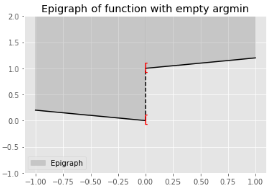
Figure 5: Example of a function that is not lower-semicontinuous at $\theta=0$.

C.2 Epi-graphical closure

The epi- (resp. hypo-) graphical closure defined below can be seen as the lower- (resp. upper-) semicontinuous regularisation of a lower-bounded function $f$. These quantities play a role in the proof of epi-convergence of Laplace functionals - see Theorem 4.1. The following can be found for instance in (Rockafellar and Wets, , 1998, Chapter 1).

Definition C.2.

Consider a function $f:\mathbb{R}^{d}\to\mathbb{R}$. We define the epigraphical closure of $f$ as the function

$$\theta\mapsto\mathrm{cl_{e}}\ f(\theta):=\inf_{\theta_{k}\to\theta}\liminf_{k}f(\theta_{k})$$

and the hypographical closure $f$ as

$$\theta\mapsto\mathrm{cl_{h}}f(\theta):=\sup_{\theta_{k}\to\theta}\limsup_{k}f(\theta_{k}).$$

Proposition C.1.

Consider a function $f:\mathbb{R}^{d}\to\mathbb{R}$. Then,

• $\mathrm{cl_{e}}f$ is lower-semicontinuous with $\mathrm{cl_{e}}f(\theta)\leq f(\theta)$

• $\mathrm{cl_{h}}f$ is upper-semicontinuous and $\mathrm{cl_{h}}f(\theta)\geq f(\theta)$.

Moreover,

• When $f$ is lower-semicontinuous, $f(\theta)=\mathrm{cl_{e}}f(\theta)$

• When $f$ is upper-semicontinuous, $f(\theta)=\mathrm{cl_{h}}f(\theta)$.

Example C.3.

Let

$$f(\theta)=\begin{cases}1,\ \theta\geq 0\\ 0,\ \theta<0\end{cases}\,.$$

Note that the function $f$ is not lower-semicontinuous. We have

$$\mathrm{cl_{e}}f(\theta)=\begin{cases}1,\ \theta>0\\ 0,\ \theta\leq 0\end{cases}\,.$$

C.3 Epi-convergence

We will need the notion of outer and inner limits of a sequence of sets, which should not be confused with the superior or inferior limits of a sequence of sets, as the latter do not assume a topological structure. We note the unfortunate traditional use of the same notation for both ideas in the literature, adopted here. This allows us to define (Painleveé-Kuratowski) convergence and hence epi-convergence and to formulate Theorem C.4, but also Propostion C.5 and Theorem C.3.

Definition C.3.

Let

$$\mathcal{N}_{\infty}^{\sharp}:=\left\{N\subset\mathbb{N};\ N\ \text{infinite}\right\}$$

be the set of all unbounded subsequences of $\mathbb{N}$, and

$$\mathcal{N}_{\infty}:=\left\{N\subset\mathbb{N};\ \mathbb{N}\setminus N\ \text{finite}\right\}$$

be the set of all subsequences of $\mathbb{N}$ containing all $n$ beyond some $\bar{n}\in\mathbb{N}$.

Definition C.4 (Outer and Inner Limits).

Let $\left\{A_{n}\subset\mathbb{R}^{d},n\in\mathbb{N}\right\}$ be a sequence of sets. We define

1. its outer limit as

   $$\mathrm{Limsup}_{n}A_{n}:=\bigcap_{N\in\mathcal{N}_{\infty}}\mathrm{cl}\bigcup_{n\in N}A_{n}$$

2. its inner limit as

   $$\mathrm{Liminf}_{n}A_{n}:=\bigcap_{N\in\mathcal{N}_{\infty}^{\sharp}}\mathrm{cl}\bigcup_{n\in N}A_{n},$$

3. when $\mathrm{Limsup}_{n}A_{n}=\mathrm{Liminf}_{n}A_{n}=:A$ then $\{A_{n},n\in\mathbb{N}\}$ is said to set-converge to $A$, denoted

   $$\mathrm{Lim}_{n}A_{n}=A,\ \ A_{n}\to A.$$

Another definition is given by the following equivalent, more intuitive, representation of inner and outer limits.

Proposition C.2.

(Rockafellar and Wets, , 1998, Section 4.A). Let $\left\{A_{n}\subset\mathbb{R}^{d},n\in\mathbb{N}\right\}$ be a sequence of sets. We have

$$\mathrm{Limsup}_{n}A_{n}=\left\{z\in\mathbb{R}^{d};\ \forall\epsilon>0\ \exists N\in\mathcal{N}_{\infty}^{\sharp},\ \forall n\in N\colon z\in A_{n}+\mathbb{B}(\epsilon)\right\}$$

$$\mathrm{Liminf}_{n}A_{n}=\left\{z\in\mathbb{R}^{d};\ \forall\epsilon>0\ \exists N\in\mathcal{N}_{\infty},\ \forall n\in N\colon z\in A_{n}+\mathbb{B}(\epsilon)\right\}$$

where $\mathbb{B}(\epsilon)$ denotes a closed metric ball of radius $\epsilon$. Moreover, it also holds that

$$\mathrm{Liminf}_{n}A_{n}=\bigcap_{\epsilon\geq 0}\Big{\{}\bigcup_{m\geq 1}\bigcap_{j\geq m}\big{[}A_{n}+\mathbb{B}(\epsilon)\big{]}\Big{\}}.$$

In words, for a sequence of sets $\left\{A_{n},\ n\in\ \mathbb{N}\right\}$ with $A_{n}\neq\varnothing$, the set $\mathrm{Liminf}_{n}A_{n}$ is the set of all possible limit points of sequences $\left\{z_{n},\ n\in\mathbb{N}\right\}$ with $z_{n}\in A_{n}$ for all $n\in\mathbb{N}$ ; the set $\mathrm{Limsup}_{n}A_{n}$ is the set of all possible cluster points of those sequences Rockafellar and Wets, (1998). As $\mathcal{N}_{\infty}\subset\mathcal{N}_{\infty}^{\sharp}$, it is clear that $\mathrm{Liminf}_{n}A_{n}\subset\mathrm{Limsup}_{n}A_{n}$. We note that the two sets are closed, and identified by the closures, in the following sense.

Proposition C.3.

(Rockafellar and Wets, , 1998, Prop. 4.4). For any sequence of sets $\left\{A_{n},\ n\in\mathbb{N}\right\}$, both $\mathrm{Limsup}_{n}A_{n}$ and $\mathrm{Liminf}_{n}A_{n}$ are closed sets. Hence, whenever $\lim_{n}A_{n}$ exists, then it is closed. In fact, if for two sequences of sets $\left\{C_{n},\ n\in\mathbb{N}\right\}$, $\left\{D_{n},\ n\in\mathbb{N}\right\}$ one has $\mathrm{cl}\,C_{n}=\mathrm{cl}\,D_{n}$, $n\in\mathbb{N}$, then $\mathrm{Liminf}_{n}C_{n}=\mathrm{Liminf}_{n}D_{n}$ and $\mathrm{Limsup}_{n}C_{n}=\mathrm{Limsup}_{n}D_{n}$.

Example C.4.

(Rockafellar and Wets, , 1998, Section 4.B)

• Let $C\subset\mathbb{R}^{d}$ with $\mathrm{cl}\,C=\mathbb{R}^{d}$. Then, the constant sequence $A_{n}=C$, $n\in\mathbb{N}$ set-converges to $\mathbb{R}^{d}$ (and not to $C$).

• Let $C_{1}$ and $C_{2}$ be distinct closed sets, and define a sequence $\left\{A_{n},\,n\in\mathbb{N}\right\}$ such that $A_{n}=C_{1}$ for $n$ odd, and $A_{n}=C_{2}$ for $n$ even. This sequence does not converge in the sense of Def. 3.4: the inner limit equals $C_{1}\cap C_{2}$, while the outer limit equals $C_{1}\cup C_{2}$.

Epi-convergence is commonly defined in terms of convergence of epigraphs.

Definition C.5.

Let $\left\{f_{n}:\mathbb{R}^{d}\to\mathbb{R},n\in\mathbb{N}\right\}$. The lower epi-limit $\mathrm{e-liminf}_{n}f_{n}$ is the function having as its epigraph the $\operatorname{Limsup}$ of the sequence of epigraphs of $\left\{f_{n},\ n\in\mathbb{N}\right\}$

$$\mathrm{epi}(\mathrm{e-liminf}_{n}f_{n})=\mathrm{Limsup}_{n}\mathrm{epi}(f_{n})$$

The upper epi-limit $\mathrm{e-limsup}_{n}f_{n}$ of the sequence is defined as the function satisfying

$$\mathrm{epi}(\mathrm{e-limsup}_{n}f_{n})=\mathrm{Liminf}_{n}\mathrm{epi}(f_{n}).$$

When for any $\theta\in\mathbb{R}^{d}$

$$(\mathrm{e-liminf}_{n}f_{n})(\theta)=(\mathrm{e-limsup}_{n}f_{n})(\theta)\,,$$

this function is called the epi-limit of $\left\{f_{n},\ n\in\mathbb{N}\right\}$. Thus,

$$f_{n}\ \text{epi-converge to}\ f\ \iff\ \mathrm{epi}(f_{n})\to\mathrm{epi}(f).$$ (34)

The following provides an intuitive characterisation of epi-convergence.

Theorem C.2 (Characterisation of epi-limits).

(Rockafellar and Wets, , 1998, Prop 7.2) Let $\left\{f_{n}:\mathbb{R}^{d}\to\mathbb{R},\ n\in\mathbb{N}\right\}$ be a sequence of functions and let $\theta\in\mathbb{R}^{d}$. We have

• $(\mathrm{e-liminf}_{n}f_{n})(\theta)=\min\left\{a\in\mathbb{R};\ \exists\theta_{n}\to\theta\ \text{with}\ \liminf_{n}f_{n}(\theta_{n})=a\right\}$

• $(\mathrm{e-limsup}_{n}f_{n})(\theta)=\min\left\{a\in\mathbb{R};\ \exists\theta_{n}\to\theta\ \text{with}\ \limsup_{n}f_{n}(\theta_{n})=a\right\}$

Thus, $\left\{f_{n},\ n\in\mathbb{N}\right\}$ epi-converge to $f$ if and only if for each $\theta\in\mathbb{R}^{d}$

• $\liminf_{n}f_{n}(\theta_{n})\geq f(\theta)$ for any $\theta_{n}\to\theta$

• $\lim_{n}f_{n}(\theta_{n})=f(\theta)$ for some sequence $\theta_{n}\to\theta$.

We can similarly characterise hypo-convergence.

Proposition C.4.

Let $\left\{f_{n}:\mathbb{R}^{d}\to\mathbb{R},\ n\in\mathbb{N}\right\}$ be a sequence of functions and let $\theta\in\mathbb{R}^{d}$. We have

$$f_{n}\ \text{hypo-converge to}\ f\ \iff\ \mathrm{hypo}(f_{n})\to\mathrm{hypo}(f).$$ (35)

We can rephrase Example 3.5 in the main text in terms of convergence of epigraphs and hypographs.

Example C.5.

We illustrate with three examples the definitions of inner and outer limit of a sequence of epigraphs and the fact that this type of convergence differs from traditional functional convergence e.g. pointwise. Consider the following examples of sequences $\left\{f_{n}\colon\mathbb{R}\rightarrow\mathbb{R},n\in\mathbb{N}\right\}$ where

• $f_{n}(\theta)=-e^{-n\theta^{2}}$ and consider the function

  $$f(\theta):=\begin{cases}-1,\ \ \theta=0\\ 0,\ \ \ \ otherwise\end{cases}\,.$$

  of epigraph the closed set

  $$\mathrm{epi}(f)=(\mathbb{R}\times\mathbb{R}_{+})\cup\left\{(0,a);\ a\geq-1\right\}\subset{\mathrm{epi}}(f_{n})\subset\mathbb{R}^{2},\forall n\in\mathbb{N},$$

  Noting that $\mathrm{epi}(f_{n+1})\subset\mathrm{epi}(f_{n})$ for any $n\in\mathbb{N}$ then for any $N\in\mathcal{N}^{\sharp}_{\infty}$ we have

  $$\bigcup_{n\in N}\mathrm{epi}(f_{n})=\mathrm{epi}(f_{\min\{N\}})=\mathrm{cl}\big{(}\mathrm{epi}(f_{\min\{N\}})\big{)}\,.$$

  Now $\mathcal{N}_{\infty}^{\sharp}=\cup_{n\in\mathbb{N}}\big{\{}N\in\mathcal{N}_{\infty}^{\sharp}\colon\min\{N\}=n\big{\}}$ and similarly $\mathcal{N}_{\infty}=\cup_{n\in\mathbb{N}}\big{\{}N\in\mathcal{N}_{\infty}\colon\min\{N\}=n\big{\}}$. Therefore

  $$\mathrm{Liminf}_{n}\mathrm{epi}(f_{n})=\mathrm{Limsup}_{n}\mathrm{epi}(f_{n})=\bigcap_{n\in\mathbb{N}}\mathrm{epi}(f_{n})\,,$$

  and, by contradiction,

  $$(\theta,a)\in{\mathrm{epi}}(f_{n})\subset\mathbb{R}^{2},\forall n\in\mathbb{N}\iff(\theta,a)\in\mathrm{epi}(f)\,,$$

  and we conclude

  $$\bigcap_{n\in\mathbb{N}}{\mathrm{epi}}(f_{n})=\mathrm{epi}(f)\,,$$

  which is closed and independent of $N\in\mathcal{N}^{\sharp}_{\infty}$. Therefore, from Def. C.4 and noting that $\mathcal{N}_{\infty}\subset\mathcal{N}_{\infty}^{\sharp}$, we have $\mathrm{Liminf}_{n}\mathrm{epi}(f_{n})=\mathrm{Limsup}_{n}\mathrm{epi}(f_{n})=\mathrm{epi}(f)$ and $\{f_{n},n\in\mathbb{N}\}$ epi-converges to $f$.

• Let $f_{n}(\theta)=e^{-n\theta^{2}}$ and consider the function $g\equiv 0$, whose epigraph is given by the closed set $\mathrm{epi}(g)=\mathbb{R}\times\mathbb{R}_{+}$. It is clear that, for an arbitrary $N\in\mathcal{N}_{\infty}^{\sharp}$,

  $$\bigcup_{n\in N}\mathrm{epi}(f_{n})=\Big{(}\mathbb{R}\times\mathbb{R}_{+}\Big{)}\setminus\Big{(}\left\{(\theta,a);\,a=0\right\}\cup\left\{(0,a);\,0\leq a<1\right\}\Big{)}\subset\mathrm{epi}(g)$$

  and it should be clear that

  $$\mathrm{cl}\bigcup_{n\in N}\mathrm{epi}(f_{n})=\mathrm{epi}(g)\,,$$

  which is independent of $N$. There, as for the previous example, the intersections involved in Def. C.4 are trivial, establishing that $\mathrm{Liminf}_{n}\mathrm{epi}(f_{n})=\mathrm{Limsup}_{n}\mathrm{epi}(f_{n})=\mathrm{epi}(g)$; hence, $\{f_{n},n\in\mathbb{N}\}$ epi-converges to $g$. The remarkable point here is that $\{f_{n},n\in\mathbb{N}\}$ does not converge pointwise to $g$, since $f_{n}(0)=1$ for all $n\in\mathbb{N}$.

• Let $f_{n}(\theta)=(-1)^{n}e^{-n\theta^{2}}$. This sequence fails to epi-converge as the set-limit does not exist. Adapting the above the inner limit $\mathrm{Liminf}_{n}\mathrm{epi}(f_{n})=\mathrm{epi}(f)$ does not coincide with the outer limit $\mathrm{Limsup}_{n}\mathrm{epi}(f_{n})=\mathrm{epi}(g)$.

We are now in a position to report set-limit results one may obtain under the assumption of epi-convergence.

Definition C.6 ($\epsilon$-optimality set).

The set of points that minimise a function $f\colon\mathbb{R}^{d}\rightarrow\mathbb{R}$ within $\epsilon\geq 0$ is denoted by

$$\epsilon-\operatorname*{argmin}f:=\left\{\theta\in\mathbb{R}^{d};\ f(\theta)\leq\underset{u\in\mathbb{R}^{d}}{\inf}f(u)+\epsilon\right\}.$$ (36)

The following result is central in the theory of convergence for procedures involving sequential minimisation of functions.

Proposition C.5 (epigraphical nesting, Rockafellar and Wets, (1998), Proposition 7.30).

Let $\left\{f_{n}:\mathbb{R}^{d}\to\mathbb{R},\ n\in\mathbb{N}\right\}$ be a sequence of functions and let $f\colon\mathbb{R}^{d}\rightarrow\mathbb{R}$.

1. If $\mathrm{e-limsup}_{n}f_{n}\leq f$, then

   $$\limsup_{n}\underset{\theta}{\inf}f_{n}(\theta)\leq\inf f.$$

2. Let $\left\{\epsilon_{n}\in\mathbb{R}_{+},\ n\in\mathbb{N}\right\}$, $\epsilon_{n}\downarrow 0$, be such that for any $\left\{\theta_{n}\in\epsilon_{n}-\operatorname*{argmin}f_{n},\ n\in\mathbb{N}\right\}$ admitting a subsequence $\left\{\theta_{n_{k}}\in\mathbb{R}^{d},\ k\in\mathbb{N}\right\}$ convergent to $\theta\in\mathbb{R}^{d}$, then it holds that $f_{n_{k}}(\theta_{n_{k}})\to_{k}f(\theta)$ and

   $$\mathrm{Limsup}_{n}\left\{\epsilon_{n}-\operatorname*{argmin}f_{n}\right\}\subset\operatorname*{argmin}f\,.$$

We can in fact obtain a stronger result when epi-convergence holds.

Theorem C.3 (Rockafellar and Wets, (1998), Theorem 7.31).

Let $\left\{f_{n}:\mathbb{R}^{d}\to\mathbb{R}\right\}$ be a sequence of functions that epi-converge to $f$, with $-\infty<\underset{u\in\mathbb{R}^{d}}{\inf}f(u)<\infty$. Then

1. For any $\epsilon>0$

   $$\mathrm{Limsup}_{n}\left\{\epsilon-\operatorname*{argmin}f_{n}\right\}\subset\epsilon-\operatorname*{argmin}f\,,$$

2. For any sequence $\left\{\epsilon_{n}\in\mathbb{R}_{+},\ n\in\mathbb{N}\right\}$, $\epsilon_{n}\downarrow 0$, we have

   $$\mathrm{Limsup}_{n}\left\{\epsilon_{n}-\operatorname*{argmin}f_{n}\right\}\subset\operatorname*{argmin}f\,.$$

An even stronger result holds when the the functions are lower-semicontinuous. Below, we say that a function $g:\mathbb{R}^{d}\to\mathbb{R}$ is eventually level-bounded if for each $a\in\mathbb{R}^{d}$ the sequence of level-sets $\left\{\mathrm{lev}_{\leq a}f_{n},\ n\in\mathbb{N}\right\}$ is eventually bounded. For instance, a sequence of eventually lower-bounded functions is eventually level-bounded. The following result is Theorem C.4 in the main text; we report it here for completeness.

Theorem C.4 (Rockafellar and Wets, (1998), Theorem 7.33).

Let

1. $f:\mathbb{R}^{d}\to\mathbb{R}$ be a lower-bounded, lower-semicontiuous function,

2. $\left\{f_{n}:\mathbb{R}^{d}\to\mathbb{R},\ n\in\mathbb{N}\right\}$ be a sequence of lower-semicontinuous functions such that

   1. $\left\{f_{n},\ n\in\mathbb{N}\right\}$ epi-converges to $f$,

   2. $\left\{f_{n},\ n\in\mathbb{N}\right\}$ is eventually level-bounded.

Then,

1. $\underset{\theta\in\mathbb{R}^{d}}{\inf}f_{n}(\theta)\to\underset{\theta\in\mathbb{R}^{d}}{\inf}f(\theta)$,

2. $\mathrm{Limsup}_{n}\operatorname*{argmin}f_{n}\subset\operatorname*{argmin}f$.

Appendix D Laplace Principle

The Laplace Principle is a known result which provides a variational representation of integrals of the form $-\log\int e^{-l(x)}\pi(x)\mathrm{d}x$, where $\pi$ is a probability density and $l$ is an integrable function.

Lemma D.1 (Laplace Principle).

Let $\nu,\pi$ be two probability measures with $\nu\ll\pi$. Let $l:\mathbb{R}^{d}\to\mathbb{R}$ be a locally integrable function such that $\int e^{-l(x)}\pi(x)\mathrm{d}x<\infty$ and set $\tilde{\pi}\propto e^{-l}\pi$ to be a probability measure. It holds that

$$\mathrm{KL}(\nu,\tilde{\pi})=\int l(x)\nu(x)\mathrm{d}x+\mathrm{KL}(\nu,\pi)+\log\int e^{-l(x)}\pi(x)\mathrm{d}x.$$ (37)

A well-known consequence is

$$\tilde{\pi}=\operatorname*{argmin}_{\nu\in\mathbb{M}^{1}_{+}(\mathbb{R}^{d})}\left\{\int l(x)\nu(x)\mathrm{d}x+\mathrm{KL}(\nu,\pi)\right\}.$$ (38)

Proof.

By direct calculations, we have

$$\mathrm{KL}(\nu,\tilde{\pi}) =\int\nu(x)\log\left(\frac{\nu(x)\pi(e^{-l})}{e^{-l(x)}\pi(x)}\right)\mathrm{d}x=$$

$$=\int\nu(x)\log\left(\frac{\nu(x)}{e^{-l(x)}\pi(x)}\right)\mathrm{d}x+\log\pi(e^{-l})$$

$$=\int\nu(x)\left\{\log(\nu(x))-\log(e^{-l(x)})-\log(\pi(x))\right\}\mathrm{d}x+\log\pi(e^{-l})$$

$$=\int\nu(x)\log\left(\frac{\nu(x)}{\pi(x)}\right)\mathrm{d}x+\int\nu(x)l(x)\mathrm{d}x+\log\pi(e^{-l})$$

which leads to equation (37). This implies

$$\operatorname*{argmin}_{\nu\in\mathbb{M}^{1}_{+}(\mathbb{R}^{d})}\left\{\int l(x)\nu(x)\mathrm{d}x+\mathrm{KL}(\nu,\pi)\right\}=\operatorname*{argmin}_{\nu\in\mathbb{M}^{1}_{+}(\mathbb{R}^{d})}\mathrm{KL}\left(\nu,\tilde{\pi}\right)=\tilde{\pi}$$

as $\mathrm{KL}(\nu,\tilde{\pi})=0$ if and only if $\nu=\tilde{\pi}$. Hence relation (38) holds.

∎

Appendix E Additional results from numerical experiments: impact of rescaling

In this section we provide additional simulations, supplementing those of Section 2. In Figure 6 we report results similar to those of Figure 2 for the Pima Indians dataset, except that, this time, the objective function $l$ is rescaled at the first iteration only. One can see that the both the exact and stochastic algorithms converge in this scenario, albeit at a slower rate (see in particular the left panel and compare with the corresponding panel in Figure 2). On the other hand, the results for the noisy (mini-batch) version look more stable.

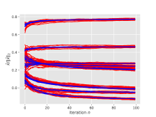
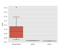
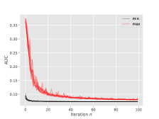
Figure 6: AUC scoring example, Pima Indians dataset, objective function $l$ is rescaled only at the first iteration. Left: Estimates of $\widehat{x}$ across iterations (blue: exact algorithm, red: minibatch algorithm). Center: box-plots (across independent runs) of final output for both algorithms, compared with Nelder-Mead with random initialisation. Right: min/max values of $l(X_{n}^{i})$ at each iteration $n$ (the different lines correspond to the different runs.)

The same strategy of rescaling $l$ at the first iteration only works poorly for the Sonar dataset (results not shown), as the estimate remains far off the solution after $4000$ iterations. We managed to achieve reasonable performance by rescaling the objective function $l$ in the first $k=400$ iterations (10% of the total number of iterations), see Figure 7. Stopping adaptation at some point leads to an algorithm that corresponds more directly to our theoretical analysis, but in practice adapting at every iteration seems to always improve the results to a certain extent.

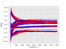
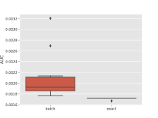
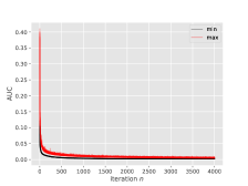
Figure 7: AUC scoring example, Sonar dataset, objective function is rescaled at each of the first $k=400$ iterations. Same plots as in Figure 6.

References

- Attouch, (1984) Attouch, H. (1984). Variational Convergence for Functions and Operators. Applicable mathematics series. Pitman Advanced Pub. Program.
- Bishop et al., (2018) Bishop, A. N., Del Moral, P., Niclas, A., et al. (2018). An introduction to Wishart matrix moments. Foundations and Trends® in Machine Learning, 11(2):97–218.
- Bolte et al., (2018) Bolte, J., Sabach, S., Teboulle, M., and Vaisbourd, Y. (2018). First order methods beyond convexity and Lipschitz gradient continuity with applications to quadratic inverse problems. SIAM Journal on Optimization, 28(3):2131–2151.
- Clémençon et al., (2008) Clémençon, S., Lugosi, G., and Vayatis, N. (2008). Ranking and Empirical Minimization of U-statistics. The Annals of Statistics, 36(2):844 – 874.
- Del Moral et al., (2006) Del Moral, P., Doucet, A., and Jasra, A. (2006). Sequential Monte Carlo samplers. Journal of the Royal Statistical Society. Series B (Statistical Methodology), 68(3):411–436.
- Ermoliev et al., (1995) Ermoliev, Y. M., Norkin, V. I., and Wets, R. J.-B. (1995). The minimization of semicontinuous functions: Mollifier subgradients. SIAM Journal on Control and Optimization, 33(1):149–167.
- Gupal and Norkin, (1977) Gupal, A. and Norkin, V. (1977). Algorithm for the minimization of discontinuous functions. Cybernetics and Systems Analysis - CYBERN SYST ANAL-ENGL TR, 13:220–223.
- Jorgensen, (1987) Jorgensen, B. (1987). Exponential dispersion models. Journal of the Royal Statistical Society. Series B (Methodological), 49(2):127–162.
- Jorgensen, (1997) Jorgensen, B. (1997). The Theory of Dispersion Models. Chapman & Hall/CRC Monographs on Statistics & Applied Probability. Taylor & Francis.
- Kleijn and van der Vaart, (2012) Kleijn, B. and van der Vaart, A. (2012). The Bernstein-Von-Mises theorem under misspecification. Electronic Journal of Statistics, 6(none):354 – 381.
- Lemieux, (2009) Lemieux, C. (2009). Monte Carlo and quasi-Monte Carlo sampling. Springer Series in Statistics. Springer, New York.
- Nesterov and Spokoiny, (2017) Nesterov, Y. and Spokoiny, V. (2017). Random gradient-free minimization of convex functions. Foundations of Computational Mathematics, 17(2):527–566.
- Nielsen and Nock, (2010) Nielsen, F. and Nock, R. (2010). Entropies and cross-entropies of exponential families. pages 3621–3624.
- Norkin, (1993) Norkin, V. I. (1993). The analysis and optimization of probability functions. Iiasa working paper, IIASA, Laxenburg, Austria.
- Osher et al., (2023) Osher, S., Heaton, H., and Fung, S. W. (2023). A Hamilton-Jacobi-based proximal operator.
- Ridgway et al., (2014) Ridgway, J., Alquier, P., Chopin, N., and Liang, F. (2014). Pac-Bayesian AUC classification and scoring. In Ghahramani, Z., Welling, M., Cortes, C., Lawrence, N., and Weinberger, K., editors, Advances in Neural Information Processing Systems, volume 27. Curran Associates, Inc.