Online Detection of Anomalies in Temporal Knowledge Graphs with Interpretability

Abstract.

Temporal knowledge graphs (TKGs) are valuable resources for capturing evolving relationships among entities, yet they are often plagued by noise, necessitating robust anomaly detection mechanisms. Existing dynamic graph anomaly detection approaches struggle to capture the rich semantics introduced by node and edge categories within TKGs, while TKG embedding methods lack interpretability, undermining the credibility of anomaly detection. Moreover, these methods falter in adapting to pattern changes and semantic drifts resulting from knowledge updates. To tackle these challenges, we introduce AnoT, an efficient TKG summarization method tailored for interpretable online anomaly detection in TKGs. AnoT begins by summarizing a TKG into a novel rule graph, enabling flexible inference of complex patterns in TKGs. When new knowledge emerges, AnoT maps it onto a node in the rule graph and traverses the rule graph recursively to derive the anomaly score of the knowledge. The traversal yields reachable nodes that furnish interpretable evidence for the validity or the anomalous of the new knowledge. Overall, AnoT embodies a detector-updater-monitor architecture, encompassing a detector for offline TKG summarization and online scoring, an updater for real-time rule graph updates based on emerging knowledge, and a monitor for estimating the approximation error of the rule graph. Experimental results on four real-world datasets demonstrate that AnoT surpasses existing methods significantly in terms of accuracy and interoperability. All of the raw datasets and the implementation of AnoT are provided in https://github.com/zjs123/ANoT.

1. Introduction

Many human activities, such as political interactions (Fan et al., 2022) and e-commerce (Liu et al., 2023c), can be effectively represented as time-evolving graphs with semantics, which are referred to as temporal knowledge graphs (TKGs). These TKGs are dynamic directed graphs characterized by node and edge categories. In this context, nodes represent entities in the real world (e.g., United States), while labeled edges signify the relations between these entities (e.g., Born In). Each edge in conjunction with its connected nodes can constitute a tuple $(s,r,o,t)$ that encapsulates a piece of real-world knowledge, where $s$ and $o$ denote the subject and object entities, $r$ denotes the relation, and $t$ represents the occurrence timestamp of the knowledge.

While TKGs have demonstrated their value across various applications (Zheng et al., 2018; Gupta et al., 2014), they often contain numerous anomalies that can significantly impede their reliability. As illustrated in Figure 1, TKG construction relies on automatic extraction from unstructured text (Zhu et al., 2023). However, existing extraction techniques often encounter conceptual confusion (Nasar et al., 2022) and inaccurate relation matching (Smirnova and Cudré-Mauroux, 2019), potentially introducing noisy tuples with erroneous entities or relations, termed as conceptual errors. Furthermore, ongoing interactions in the real world lead to the formation of new knowledge or render existing knowledge obsolete. However, knowledge-updating processes are often insufficient and delayed (Tang et al., 2019), resulting in either the omission of new knowledge or the retention of invalid knowledge, termed missing errors and time errors. Specifically, these errors are indicated by their conflicts with preserved knowledge. Conceptual errors conflict with the interaction preference of entities, while time errors conflict with other timely updated knowledge in their time order. The missing errors are valid knowledge not included in TKGs and should have few conflicts. TKG anomaly detection refers to detecting conceptual, time, and missing errors by measuring conflicts. Unfortunately, this field receives little attention.

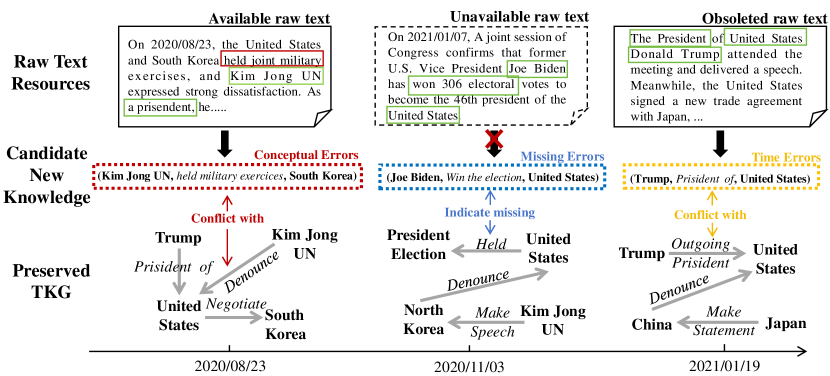
Figure 1. An illustration of different types of anomalies in TKGs and how anomalies relate to preserved knowledge.

One closely related research field is dynamic graph anomaly detection (Salehi and Rashidi, 2018), aimed at identifying abnormal connections in time-evolving graphs. However, existing methods primarily rely on simple structural properties, such as connectivity (Aggarwal et al., 2011) or clusters (Manzoor et al., 2016), thus failing to capture the intricate patterns present in TKGs such as relational closures (Zhang et al., 2022) and temporal paths (Fan et al., 2022). Furthermore, these methods do not consider the semantic attributes of nodes and are thus ineffective in handling the rich semantics introduced by node and edge categories. Another related field is TKG embedding (Wang et al., 2023), which aims to represent entities and relations as low-dimensional vectors for downstream tasks such as link prediction (Rossi et al., 2022). While these vectors can also be utilized for anomaly scoring (Jia et al., 2019), they face limitations due to the requirement of substantial training data (Gao et al., 2019) and the absence of interpretability (Jung et al., 2021), making their anomaly detection less convincing. Moreover, the semantics of entities and graph patterns change as TKGs continue to update. Since these methods learn fixed vectors, they struggle to adapt to online changes. In summary, TKG anomaly detection encounters three primary challenges: CH1. Be interpretable to provide evidence for the detection results; CH2. Capturing complex patterns arising from entity and relation semantics and temporal relevance; CH3. Handling semantic and pattern changes caused by knowledge updates.

In this paper, we propose AnoT, a novel TKG summarization method for online detection of anomalies. It distills TKG into an interpretable rule graph and walks on it to gather evidence of knowledge validity. For CH1, AnoT conceptualizes observed knowledge as atomic rules, distilling interaction patterns within TKGs into concept triples that are both concise and human-readable. By mapping new knowledge as atomic rules, they can interpret how new knowledge complies or conflicts with existing patterns, and thus give evidence of the decision. Moreover, by identifying these discrepancies, AnoT can offer guidelines on correcting anomalous knowledge. For CH2, AnoT advances the utility of atomic rules by associating them through two common occurring relationships: chain and triadic occurrence. We formulate this association results as a rule graph, with nodes representing interaction patterns and directed edges indicating their sequential relationships. This novel structure enables the flexible inference of complex patterns by walking on it. For CH3, given the rule graph, the semantic and pattern changes can be easily reformed as editions on its nodes and edges, which provides a precise and scalable method for uniformly managing online changes. Additionally, we propose an error approximation strategy to determine the refresh time of the rule graph. Conceptually, AnoT is composed of three elements: a detector that constructs the rule graph and evaluates new knowledge, an updater that revises the rule graph based on new knowledge, and a monitor that estimates the rule graph’s availability. Based on the rule graph, we propose static scores (measuring interaction preference conflicts) to detect conceptual errors and temporal scores (measuring occurrence order conflicts) to detect time errors. Consequently, the missing errors can be filtered as knowledge with low static and time scores during walking on the rule graph. Our contributions are as follows:

• To the best of our knowledge, we are the first to study anomaly detection for TKGs. We propose an accurate and interpretable solution AnoT for this problem.

• We are the first to study the method and application of TKG summarization. We propose the rule graph to effectively summarize TKGs, and verify its usage in anomaly detection.

• Extensive experiments on four real-world TKGs justify that ANoT can accurately detect anomalies with efficiency while being interpretable. It outperforms existing methods by an average of 11.5% in AUC and 13.6% in precision.

2. Related Work

Dynamic graph anomaly detection.

Existing methods fall into two categories. One is statistical methods, which leverage the shallow mechanisms to extract the structural information (Eswaran and Faloutsos, 2018; Ranshous et al., 2016; Manzoor et al., 2016; Eswaran et al., 2018). For example, CAD (Sricharan and Das, 2014) detects abnormal edges by tracking changes in structure and weight. DynAnom (Guo et al., 2022) uses the dynamic forward push algorithm to calculate the personalized PageRank vector for each node. AnoGraph (Bhatia et al., 2023) extends the count-min sketch data structure to detect anomalous edges through dense subgraph searches. F-FADE (Chang et al., 2021) models the time-evolving distributions of node interactions using frequency factorization. However, they cannot capture complex patterns brought by entity and relation semantics in TKGs. The other is deep learning-based methods, which detect anomalies by learning vector representations for nodes (Liu et al., 2023a; Fan et al., 2020; Belle et al., 2022; Zheng et al., 2019). AEGIS (Ding et al., 2020) proposes a graph differentiation network to learn node representations. Netwalk (Yu et al., 2018) combines random walk and a dynamic clustering-based model to score anomalies. AER (Fang et al., 2023) uses an anonymous representation strategy to identify edges by their local structures. TADDY (Liu et al., 2023a) uses a dynamic graph transformer model to aggregate spatial and temporal information. However, they lack enough high-quality labels (Gao et al., 2019) and the learned representations are not interpretable, making their detection less convincing.

TKG embedding.

Factorization-based methods (Zhang et al., 2024; Yang et al., 2024; Wang et al., 2023) regard TKGs as 4-order tensors and use tensor factorization for embeddings. TNT (Lacroix et al., 2020) builds on the complex vector model ComplEx (Trouillon et al., 2017) with temporal regularization. Timeplex (Jain et al., 2020) extends TNT by capturing the recurrent nature of relations. TELM (Xu et al., 2021) learns multi-vector representations with canonical decomposition. However, they learn tensors with fixed shapes, limiting their ability to handle new entities and timestamps. Diachronic embedding-based methods (Dasgupta et al., 2018; Xu et al., 2020b) model entity representations as time-related functions. DE-simple (Goel et al., 2020) uses nonlinear operations to model various evolution trends of entity semantics. ATiSE (Xu et al., 2020a) uses multi-dimensional Gaussian distributions to model the uncertainty of entity semantics. TA-DistMult (García-Durán et al., 2018) uses a sequence model for time-specific relation representations. However, they over-simplify the evolution of TKG and ignore the graph structure. GNN-based methods (Park et al., 2022; Ren et al., 2023; Liu et al., 2023b) employ the message-passing mechanism to simulate the entity interactions. TeMP (Wu et al., 2020) uses self-attention to model the spatial and temporal locality. RE-GCN (Li et al., 2021) auto-regressively models historical sequence and imposes attribute constraints on entity representations. However, they lack interpretability and cannot handle online changes.

Graph summarization.

Graph summarization is closely related to anomaly detection since it aims to find general patterns in data, and thus in turn can reveal anomalies (Belth et al., 2020b; Cebiric et al., 2019). Many studies on knowledge graph summarization have focused on query-related summaries (Wu et al., 2013) and personalized summaries (Safavi et al., 2019), while KGist (Belth et al., 2020b) learns inductive summaries by introducing root graphs. However, they ignore the temporality of knowledge. Recent efforts have focused on dynamic graph summarization (Hajiabadi et al., 2022). TimeCrunch (Shah et al., 2015) uses temporal phrases to describe the temporal connectivity. PENminer (Belth et al., 2020a) mines activity snippets’ persistence in evolving networks. However, they only focus on evolving connectivity and fail to handle rich semantics in TKGs. In this paper, we propose AnoT, a scalable and information-theoretic method for inductive TKG summarization.

3. Preliminaries

3.1. Temporal Knowledge Graph

A temporal knowledge graph is denoted as $\mathcal{G}=(\mathcal{E},\mathcal{R},\mathcal{T},\mathcal{F})$. $\mathcal{E}$ and $\mathcal{R}$ are entity set and relation set, respectively. $\mathcal{T}$ is the set of observed timestamps and $\mathcal{F}$ is the set of facts. In real-world scenarios, $\mathcal{E}$, $\mathcal{T}$, and $\mathcal{F}$ will be continuously enriched. Each tuple $(s,r,o,t)\in\mathcal{F}$ connects the subject and object entities $s,o\in\mathcal{E}$ via a relation $r\in\mathcal{R}$ in timestamp $t\in\mathcal{T}$, which means a unit knowledge (i.e., a fact). We represent the connectivity of $\mathcal{G}$ in each timestamp $t$ with a $|\mathcal{E}|\times|\mathcal{E}|\times|\mathcal{R}|$ adjacency tensor $A_{t}$, where 1 represents that the entities are connected by the relation in timestamp $t$. There are two common occurring relationships exist in TKGs. One is chain occurring defined as $\{(s,r_{i},o,t_{i})\rightarrow(s,r_{j},o,t_{j})|t_{j}\geq t_{i}\}$, e.g., $(Obama,WintheSelection,UnitedStates,2008/11/04)\rightarrow(Obama,Presidentof,UnitedStates,2009/01/20)$. The other is triadic occurring defined as $\{((s,r_{i},$ $o,t_{i}),(s,r_{j},p,t_{j}))\rightarrow(o,r_{k},p,t_{k})|t_{k}\geq max(t_{i},t_{j})\}$, e.g., $((China,HostVisit,SaudiArabia,2023/03/$ $06),(China,HostVisit,Iran,2023/03/06)\rightarrow(SaudiArabia,SignAgreement,Iran,2023/03/10)$. The facts on the left of the arrow are called head facts, and those on the right are called tail facts.

3.2. Anomalies in TKGs

Here, we formally define three kinds of typical anomalies in TKGs. Given a TKG $\mathcal{G}$, we first define its corresponding ideal TKG as $\hat{\mathcal{G}}=(\mathcal{E},\mathcal{R},\mathcal{T},\hat{\mathcal{F}})$ which removes all the incorrect facts from $\mathcal{F}$ and complete all the missing facts into $\mathcal{F}$ (i.e., $(s,r,o,t)\in\hat{\mathcal{F}}$ if and only if it holds in reality). We further define the ideal triple set $\hat{\mathcal{L}}=\{(s,r,o)|(s,r,o,t)\in\hat{\mathcal{F}}\}$. Note that, $\hat{\mathcal{G}}$ and $\hat{\mathcal{L}}$ are only conceptual aids that do not exist. We then use it to define anomalies.

3.2.1. Conceptual Errors.

Extraction methods may introduce noised facts with error entities or relations in TKGs. Formally, we define the conceptual errors as $\mathcal{F}_{c}=\{(s_{c},r_{c},o_{c},t_{c})|(s_{c},r_{c},o_{c},t_{c})\in\mathcal{F},(s_{c},r_{c},o_{c})\notin\hat{\mathcal{L}}\}$, e.g., $(JoeBiden,BornIn,Ireland,1942/11/20)$.

3.2.2. Time Errors.

Knowledge updating may make existing facts invalid, but update delays will let these invalid facts not be removed from TKGs. Formally, we define the time errors as $\mathcal{F}_{t}=\{(s_{t},r_{t},o_{t},t_{t})|(s_{t},r_{t},o_{t},t_{t})\in\mathcal{F},(s_{t},r_{t},o_{t})\in\hat{\mathcal{L}},(s_{t},r_{t},o_{t},t_{t})\notin\hat{\mathcal{F}}\}$. For example, $(Obama,President$ $of,UnitedStates,2023/10/21)$.

3.2.3. Missing Errors.

Insufficient updates also prevent some correct facts not being added to TKGs. Formally, we define the missing errors as $\mathcal{F}_{m}=\{(s_{m},r_{m},o_{m},t_{m})|(s_{m},r_{m},o_{m},t_{m})\notin\mathcal{F},(s_{m},r_{m},o_{m},$ $t_{m})\in\hat{\mathcal{F}}\}$. For instance, a TKG might include the knowledge Barack Obama left office but lack his inauguration. Unlike TKG completion that predicts missing entities or relations for given tuples, we aim to find which tuple is missing in TKG. Note that these anomalies will persist as TKGs keep growing in real-world situations.

3.3. Minimum Description Length Principle

In the two-part minimum description length (MDL) principle (Rissanen, 1978), given a set of models $\mathcal{M}$, the best model $M\in\mathcal{M}$ on data $D$ minimizes $L(M)+L(D|M)$, where $L(M)$ is the length (in bits) of the description of $M$, and $L(D|M)$ is the length of the description of the data when encoded using $M$. In this work, we leverage MDL to find the optimal summarization model of a given TKG. Each MDL-based approach must devise its definitions for the description lengths, and here we follow the most commonly used primitives (Galbrun, 2022).

3.4. Summarization of A TKG

The summarization of a graph is a more refined and compact representation of the graph (Blasi et al., 2022), including super-graphs (Chen et al., 2009), sparsified graphs (Maccioni and Abadi, 2016), and independent rules (Shah et al., 2015). However, they fail to handle rich semantics and temporal relevance in TKGs, inspiring us to propose a novel rule graph as the summarization of a TKG.

3.4.1. Atomic Rules.

Given a TKG $\mathcal{G}$, we first construct a function $\mathcal{C}(\cdot)$, which takes each entity as input and outputs its category. Based on this, each knowledge $(s,r,o,t)\in\mathcal{G}$ can be mapped as an atomic rule $(\mathcal{C}(s),r,\mathcal{C}(o))$, which summarizes the interaction pattern of the knowledge (e.g., $(Obama,Win,NobelPeacePrize,2019/10/09)$ can be mapped as $(PERSON,Win,PRIZE)$).

3.4.2. Rule Graph.

A rule graph is a directed graph $\mathrm{G}=\{\mathrm{V},\mathrm{E}\}$, where each $v\in\mathrm{V}$ is a node indicating an atomic rule, and each $e\in\mathrm{E}$ is a rule edge preserving the sequential relevance between atomic rules. There are two kinds of rule edges in $\mathrm{E}$. One is derived from the chain occurring (e.g., $(PERSON,Nominated,PRIZE)\rightarrow(PERSON,Win,PRIZE)$), termed as $(v_{h}\rightarrow v_{t})$ where $v_{h}$ is the head atomic rule and $v_{t}$ is the tail atomic rule. The other is derived from the triadic occurring (e.g., $(PERSON,Write,BOOK),(BOOK$, $Nominated,PRIZE)\rightarrow(PERSON,Win,PRIZE)$), termed as $((v_{h},$ $v_{m})\rightarrow v_{t})$, where $v_{m}$ is the middle atomic rule. By associating atomic rules with rule edges, paths between atomic rules can describe the occurrence relevance between two kinds of interactions.

3.5. Problem Definition

Detecting anomalies for TKGs that have been offline preserved in the database is meaningful. However, it is a more valuable but difficult problem to detect anomalies for TKGs that are online updating, requiring the model to be efficient, adaptive to online changes, and easy to rebuild. We term it inductive anomaly detection in TKGs.

Definition 3.1 (Inductive anomaly detection in TKGs).

Given an online updating TKG $\mathcal{G}$ where the most recently updated timestamp is $t_{e}$, inductive anomaly detection aims to construct a model $M$ based on $\mathcal{G}$ to find anomalies in the future timestamps $t>t_{e}$. It contains classifying whether each newly arrived knowledge $(s,r,o,t)$ is an anomaly (i.e., conceptual or time errors), and determining whether some knowledge is missing in $t$ (i.e., missing error).

We leverage the widely used compression principle MDL to construct $M$, which follows the idea of compression in information theory to find general patterns to describe the valid data, and thus in turn reveal anomalies. The sub-problem is hence defined as:

Definition 3.2 (Inductive TKG summarization with MDL).

Given an online updating TKG $\mathcal{G}$, we seek to find the model $M^{*}$ (i.e., the optimal rule graph) that minimizes the description length of $\mathcal{G}$,

(1) $$M^{*}=\mathop{\arg\min}_{M\in\mathcal{M}}\{L(M)+L(\mathcal{G}|M)\}.$$

With the constant enrichment of $\mathcal{G}$, $M^{*}$ varies across timestamps. However, it is time-consuming to construct $M^{*}$ from scratch in every timestamp, requiring a strategy to update $M^{*}$ incrementally.

4. Method

4.1. Overview

Motivation.

Reflecting on the challenges in TKG anomaly detection, we recognize that a rule-based summarization approach could effectively tackle these issues. First, rules encapsulate the most common patterns within a graph in a human-readable form. If we can map new knowledge as a set of rules, then they can provide interpretable evidence for its validity. Second, the complex patterns observed in TKGs stem from the composition of simpler, independent patterns. If we can appropriately link these simple rules, then the complex patterns can be flexibly deduced based on the individual rules. Last, rules describe the properties of a TKG in a more compact and refined way. Thus ideally, any semantic and pattern shifts can be described as modifications of the rules.

Solution.

In this paper, we propose AnoT, a novel summarization method for TKG anomaly detection. As depicted in Figure 2, AnoT takes an online updating TKG as input, identifies anomalies, and then filters valid knowledge. The process initiates with the detector module, which constructs a rule graph based on the offline preserved part of TKG. Upon the arrival of new knowledge, this module evaluates it against the rule graph to compute an anomaly score. Subsequently, the updater module receives valid knowledge identified by the detector module, and then reforms them as edit operations on the rule graph to handle online semantic and pattern changes. The monitor module estimates the approximate error of the rule graph in representing the TKG. When the approximate error exceeds the threshold, the monitor will inform the detector to refresh the rule graph based on the current TKG. In this way, the reachable nodes during walking will give readable evidence for detection, while the complex patterns can be flexibly described by the walking paths, and the online changes are uniformly handled.

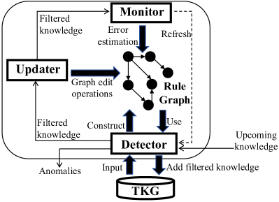
Figure 2. Conceptual illustration of the proposed AnoT framework.

In the following, we first define the description length of $\mathcal{G}$ used to find the optimal rule graph, and then detail each part of AnoT.

4.2. Description Length of The Rule Graph

We employ the minimum description length principle to guide the construction of the optimal rule graph. In other words, we consider it as a classic information-theoretic transmitter/receiver setting (Wang et al., 2020), where the goal is to describe the graph to the receiver using as few bits as possible. As a result, we should first define the number of bits required to describe the TKG (i.e., $L(M)$ and $L(\mathcal{G}|M)$).

4.2.1. $L(M)$.

Based on the primitives of MDL principle (Galbrun, 2022) and the definition of the rule graph, the encoding cost of a rule graph $\mathrm{G}=\{\mathrm{V},\mathrm{E}\}$ consists of the number of atomic rules $\mathrm{V}$, the number of rule edges $\mathrm{E}$ (both upper bounded by the number of possible candidates), and the encoding cost of $V$ and $E$, which is defined as

(2) $$\begin{split}L(M)=log(2*|\mathcal{C}_{\mathcal{E}}|^{2}*|\mathcal{R}|)+log\binom{2*|\mathcal{C}_{\mathcal{E}}|^{2}*|\mathcal{R}|}{3}+\sum_{v\in\mathrm{V}}L(v)+\sum_{e\in\mathrm{E}}L(e),\end{split}$$

where the first term is the upper bound of the number of candidate atomic rules. $|\mathcal{C}_{\mathcal{E}}|$ is the total number of entity categories derived from function $\mathcal{C}(\cdot)$ (see Section 4.3.1). $|\mathcal{R}|$ is the number of relations. Each atomic rule has the form of (CATEGORY, relation, CATEGORY), and thus results in $|\mathcal{C}_{\mathcal{E}}|^{2}*|\mathcal{R}|$. Twice because each relation has two directions. The second term is the upper bound of the number of candidate rule edges, where $log\binom{A}{B}$ means the description length of uniformly choosing $B$ elements from $A$ elements. Each rule edge associates two or three atomic rules (i.e., chain or triadic occurring), and thus results in $B$=3 as the upper bound. $L(v)$ and $L(e)$ are respectively the encoding costs of each atomic rule and each rule edge, defined as

(3) $$\begin{split}L(v)=log|\mathcal{C}_{\mathcal{E}}|+(-log\frac{n^{c_{s}}}{|\mathcal{E}|})+(-log\frac{n^{c_{o}}}{|\mathcal{E}|})+(-log\frac{n^{r}}{|\mathcal{F}|}+1),\end{split}$$

where the first term is the number of the categories of entities. The second to fourth terms are the number of bits used to encode subject categories, object categories, and relations respectively. Note that we use optimal prefix code (Huffman, 1952) to encode actual categories, so $n^{c_{s}}$ is the number of times category $c_{s}\in\mathcal{C}_{\mathcal{E}}$ occurs in $\mathcal{G}$ ($n^{c_{o}}$ is similar), while $n^{r}$ is the number of times relation $r\in\mathcal{R}$ occurs in $\mathcal{G}$ and $1$ represents the direction of the relation. Since the number of relations is constant across different models, we ignore it during model selection. We define the encoding cost of each rule edge as

(4) $$\begin{split}L(e)=log|\mathrm{E}|+(-log\frac{n^{v_{h}}}{|\mathrm{E}|})+(-log\frac{n^{v_{m}}}{|\mathrm{E}|})+(-log\frac{n^{v_{t}}}{|\mathrm{E}|})+1,\end{split}$$

where $|\mathrm{E}|$ is the number of the rule edges and $n^{v_{h}}$ is the number of head atomic rule $v_{h}$ occurs in rule graph $\mathrm{G}$. $1$ represents the direction of the edge. Note that for brevity, we only give $L(e)$ of the triadic occurring and the chain occurring can be easily extended by removing the auxiliary atomic rule part (i.e., the third term).

4.2.2. $L(\mathcal{G}|M)$.

Each atomic rule can describe a set of facts in TKG (e.g., atomic rule $(PERSON,Wins,$ $PRIZE)$ can describe fact $(Obama,Win,NobelPeacePrize,2019/10/09)$), and each rule edge can describe a set of occurring relationships among facts. For example, rule edge $(PERSON,WintheSelection,$ $COUNTRY)\rightarrow(PERSON,Presidentof,COUNTRY)$ can describe the relationship that fact $(Obama,$ $Presidentof,UnitedStates,2009/01/20)$ occurs subsequently after the fact $(Obama,WintheSelection,$ $UnitedStates,2008/11/04)$. These described facts are called correct assertions. They can be encoded by the given rule graph. Moreover, TKGs inevitably contain noise and uncommon facts and thus there may be facts that cannot be encoded by the rule graph, called negative errors. Therefore, the encoding cost of $\mathcal{G}$ by the rule graph $M$ is $L(\mathcal{G}|M)=L(\mathcal{A}^{\mathcal{G}})+L(\mathcal{N}^{\mathcal{G}})$. $L(\mathcal{A}^{\mathcal{G}})$ is the encoding cost of the correct assertions and $L(\mathcal{N}^{\mathcal{G}})$ is the encoding cost of the negative errors. The encoding cost of the correct assertions is defined as

(5) $$\begin{split}L(\mathcal{A}^{\mathcal{G}})=\sum_{v\in V}\sum_{a_{v}\in\mathcal{A}_{v}^{\mathcal{G}}}L(a_{v})+\sum_{e\in E}\sum_{a_{e}\in\mathcal{A}_{e}^{\mathcal{G}}}L(a_{e}),\end{split}$$

where $\mathcal{A}_{v}^{\mathcal{G}}$ and $\mathcal{A}_{e}^{\mathcal{G}}$ are the sets of correct assertions of each atomic rule $v$ and each rule edge $e$ respectively. $L(a_{v})$ and $L(a_{e})$ are respectively the encoding costs of fact $a_{v}$ (i.e., a correct assertion of $v$) and relationship $a_{e}$ (i.e., a correct assertion of $e$), defined as

(6) $$\begin{split}L(a_{v})=(-log\frac{n^{s_{v}}}{|\mathcal{A}_{v}^{\mathcal{G}}|})+(-log\frac{n^{o_{v}}}{|\mathcal{A}_{v}^{\mathcal{G}}|}),\end{split}$$

(7) $$\begin{split}L(a_{e})=(-log\frac{n^{a^{h}_{e}}}{|\mathcal{A}_{e}^{\mathcal{G}}|})+(-log\frac{n^{a^{m}_{e}}}{|\mathcal{A}_{e}^{\mathcal{G}}|})+(-log\frac{n^{a^{t}_{e}}}{|\mathcal{A}_{e}^{\mathcal{G}}|}),\end{split}$$

where $n^{s_{v}}$ and $n^{o_{v}}$ are respectively the numbers of times entity $s$ and $o$ occur in all the correct assertions of atomic rule $v$ (i.e., $\mathcal{A}_{v}^{\mathcal{G}}$). Note that the encoding cost of the relation is ignored since it has been included in $L(v)$. $a^{h}_{e}$, $a^{m}_{e}$, and $a^{t}_{e}$ are respectively the head fact, middle fact, and the tail fact of $a_{e}$, and thus $n^{a^{h}_{e}}$ is the number of times fact $a^{h}_{e}$ occurs in all the correct assertions of rule edge $e$ (i.e., $\mathcal{A}_{e}^{\mathcal{G}}$). $a^{m}_{e}$ and $a^{t}_{e}$ are defined similarly.

The negative errors contain two parts: the facts that cannot be mapped into any atomic rules, and the facts that can be mapped but cannot be associated with any other facts. Given the adjacency tensor $A_{t}$ of each timestamp, the unmodeled facts can be defined as $A_{t}^{-}=A_{t}-A_{t}^{m}$. $A_{t}^{m}$ is a subset of $A_{t}$ where each element is set as 1 if 1) it is 1 in $A_{t}$; 2) the corresponding fact can be mapped into atomic rules; and 3) the corresponding fact can be associated with a previous fact in $t^{\prime}<t$ via the rule edges. Since the number of missing facts can be inferred given the total number of facts and the number of facts that are already explained by the model, we only consider the cost of encoding the positions of 1 in $A_{t}^{-}$. The encoding cost of the negative errors can be then defined as

(8) $$\begin{split}L(\mathcal{N}^{\mathcal{G}})=\sum_{t\in\mathcal{T}}log\binom{|{\mathcal{E}}|^{2}*|\mathcal{R}|-|A_{t}^{m}|}{|A_{t}^{-}|},\end{split}$$

where $|\cdot|$ is set cardinality and the number of 1s in a tensor. As the above definitions give us a reliable way to measure the quality of summarizing a TKG, we then aim to find the best TKG summarization model by minimizing such description length.

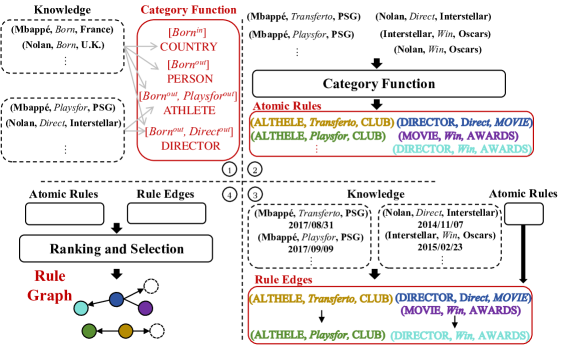
Figure 3. Rule graph construction, which contains: 1. Category function construction, 2. Generating candidate atomic rules, 3. Generating candidate rule edges, 4. Ranking and selecting.

4.3. Detector

The detector module has two functions: 1) Construct the optimal rule graph. As shown in Figure 3, a category function is first constructed based on existing knowledge (Section 4.3.1), and then it will be used to map knowledge as candidate atomic rules and candidate rule edges (Section 4.3.2). Finally, the most expressive candidates will be iteratively selected to construct the rule graph (Section 4.3.3). More details can be found in Algorithm 1. 2) Generate anomaly scores. As shown in the upper part of Figure 4, new knowledge will be first mapped as a set of atomic rules. Atomic rules that exist in the rule graph can give evidence of their conceptual validity, which will derive the static scores (Section 4.3.4). Then, the evidence of time validity is gathered by recursively walking on the rule graph and instantiating the processor nodes, which will derive the temporal scores. More details can be found in Algorithm 2.

Algorithm 1 Construct the rule graph

1:Input: Offline preserved part of TKG $\mathcal{G}$

2:Output: A model $M^{*}$ consisting of atomic rules and rule edges

3:Read $\mathcal{G}$ and construct the category function $\triangleright$ 4.3.1

4:Generate candidate atomic rules $\mathcal{P}(v)$ and candidate rule edges $\mathcal{P}(e)$ based on $\mathcal{G}$ and the category function $\triangleright$ 4.3.2

5:Rank all $v\in\mathcal{P}(v)$ first by $\Delta L(\mathcal{G}|M\cup\{v\})\downarrow$ then by $|\mathcal{A}_{v}^{\mathcal{G}}|\downarrow$ and finally by $ID\downarrow$ $\triangleright$ 4.3.3

6:Rank all $e\in\mathcal{P}(e)$ first by $\Delta L(\mathcal{G}|M\cup\{e\})\downarrow$ then by $|\mathcal{A}_{e}^{\mathcal{G}}|\downarrow$ and finally by $ID\downarrow$ $\triangleright$ 4.3.3

7:$M^{*}\leftarrow\emptyset$

8:while not converged do $\triangleright$ 4.3.3

9:    for $v\in\mathcal{P}(v)$ do

10:        if $L(\mathcal{G}|M^{*}\cup{v})<L(\mathcal{G}|M^{*})$  then

11:           $M^{*}\leftarrow M^{*}\cup{v}$ $\triangleright$ add more $v$ to $M^{*}$             

12:    for $e\in\mathcal{P}(e)$ do

13:        if $L(\mathcal{G}|M^{*}\cup{e})<L(\mathcal{G}|M^{*})$  then

14:           $M^{*}\leftarrow M^{*}\cup{e}$ $\triangleright$ add more $e$ to $M^{*}$             

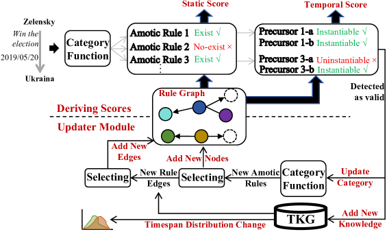
Figure 4. Conceptual illustrations of the scoring process and the updater module.

4.3.1. Construct Category Function.

Entity categories are often missing in real-world TKGs (You et al., 2020). Fortunately, we find that the category of an entity is largely related to the relations it interacts with. For example, an entity that interacts with relations $BornIn$ and $PlaysFor$ should have a category of $ATHLETE$, and an entity that interacts with relations $BornIn$ and $Create$ can be an $ARTIST$. Intuitively, the more relations are considered, the more fine-grained information a category can imply. This inspires us to generate categories for entities by extracting the frequent relation combinations. A relation combination occurs more frequently across entities means it can describe a more general property shared by entities, which is more likely to imply a category.

Formally, we define the interaction relation set of an entity $e\in\mathcal{E}$ as $R(e)=\{r|(e,r,o,t)\in\mathcal{F}\}$. With each entity providing a relation set, we then use the PrefixSpan algorithm (Pei et al., 2001) to find the most frequent subset within $R(e)$ across all entities. Each identified subset is a frequent relation combination that suggests a potential category. Subsets encompassing more relations imply more granular categories. However, finding frequent subsets with large sizes is very time-consuming. To counterbalance efficiency with categories’ quality, we propose to only find small relation combinations (i.e., up to 3 relations) and then iteratively aggregate selected subsets. Let the output of PrefixSpan be $\textbf{R}=\{(R_{1},E_{1}),(R_{2},E_{2}),...\}$, where $R_{i}$ is the ith most frequent relation combination $(r_{i}^{1},r_{i}^{2},r_{i}^{3})$ and $E_{i}=\{e|e\in\mathcal{E},R_{i}\subseteq R(e)\}$ is the entities encompassed by $R_{i}$. We commence with entity-based aggregation: if a significant overlap exists between entities in $E_{i}$ and $E_{j}$ (exceeding 90%), it indicates shared properties that necessitate simultaneous description via both relation combinations. Consequently, we introduce $(R=R_{i}\cup R_{j},E=E_{i}\cap E_{j})$ into R as a more fine-grained category. We then perform relation-based aggregation: if a significant overlap exists between relations in $R_{m}$ and $R_{n}$ (exceeding 90%), it means the categories implied by $R_{m}$ and $R_{n}$ are very similar. Therefore, we add $(R=R_{m}\cap R_{n},E=E_{m}\cup E_{n})$ into R as a more generalizable category. These aggregation steps are circularly executed until no further combinations can be aggregated. Following this phase, each relation combination $R_{i}$ is conceptualized as an implicit category $c_{i}$, with the respective entities in $E_{i}$ being categorized accordingly. To reduce category redundancy, we sort the relation combinations in descending order of the number of their covered entities and select one by one until each entity has at least $k$ categories.

4.3.2. Candidate Generation.

To construct the rule graph, we should first generate all possible rules and rule edges as candidates based on the input TKG. For each fact $(s,r,o,t)$, we generate the corresponding candidate atomic rules as $\{(c_{i},r,c_{j})|c_{i}\in C(s),c_{j}\in C(o)\}$, where $C(s)$ is the category set of $s$. We gather the rules derived from all facts $(s,r,o,t)\in\mathcal{F}$ as the candidate set of atomic rules.

To generate all possible chain-occurring-based rule edges, we first construct the interaction sequence $S(s,o)=\{r_{1},r_{2},...\}$ for each entity pair appeared in $\mathcal{G}$. The interaction sequence preserves all the relations that occurred between $s$ and $o$ and is sorted by the ascending order of their occurrence timestamps. Thus, any adjacent relations in the sequence represent two interactions between $s$ and $o$ that occur successively, which may imply a chain-occurring pattern. Formally, given each entity pair $(s,o)$ and its corresponding interaction sequence, we generate the candidate rule edges as $\{(c_{s},r_{m},c_{o})\rightarrow(c_{s},r_{n},c_{o})|c_{s}\in C(s),c_{o}\in C(o),r_{m},r_{n}\in S(s,o),m<n\}$. We gather the rule edges derived from all entity pairs that appear in $\mathcal{G}$ as the candidate set of chain-occurring-based rule edges. Since the occurrence timespan between different relations may vary, e.g., $MakeStatement$ may occur a few days after $WintheElection$, but $Retirement$ may occur several years later, considering the timespan of occurrence between two relations assists in determining the occurrence of a fact at a particular timestamp. Therefore, we also preserve the occurrence timespans of facts for each rule edge $e$ (e.g., $t_{n}-t_{m}$ for chain-occurring facts $(s,r_{m},o,t_{m})$ and $(s,r_{n},o,t_{n})$) and results in a timespan set $T(e)$.

For triadic-occurring-based rule edges, in each timestamp $t\in\mathcal{T}$, we find facts that occur at $t$ and share one same entity (e.g., $(s,r_{m},o,t)$ and $(h,r_{n},o,t)$). Then, we find the most closely occurred fact in $t_{p}\geq t$ that contains $s$ and $h$ (e.g., $(s,r_{p},h,t+3)$). These three facts describe the formation process of a triadic closure, which may imply a triadic-occurring pattern. Since there is local randomness in the occurrence time of facts (Mondal and Deshpande, 2012), we relax the same time restriction of the former two facts as co-occurring within a short period. Formally, for each timestamp $t$, the triadic-occurring-based candidate rule edges are generated as $\{((c_{s},r_{m},c_{o}),(c_{h},r_{n},c_{o}))\rightarrow(c_{s},r_{p},c_{h})|c_{s}\in C(s),c_{o}\in C(o),c_{h}\in C(h),|\mathcal{T}(e_{s},r_{m},e_{o})-t|\leq L,|\mathcal{T}(e_{h},r_{n},e_{o})-t|\leq L,\mathcal{T}(e_{s},r_{p},e_{h})\geq t+L\}$, where $\mathcal{T}(\cdot)$ is the occurrence timestamp of fact and $L$ is a hyperparameter. We also preserve the occurrence timespans for these facts.

4.3.3. Ranking and Selection.

We propose a greedy approach to select the most representative candidate into the rule graph iteratively. Our objective is to select the candidate that leads to the largest encoding cost reduction in each iteration. Recognizing that varying orders of selection may yield inconsistent models, thus affecting reproducibility, we implement a structured ranking mechanism that ensures a consistent selection order of candidates. Since the more a candidate can reduce negative errors, the more valuable it might be, we first rank candidates based on the descending order of their error reduction $\Delta L(\mathcal{G}|M\cup\{x\})=L(\mathcal{G}|M)-L(\mathcal{G}|M\cup\{x\})$, where $x$ represents candidate atomic rule $v$ or rule edge $e$. The ties in the ranking are broken by selecting candidates with more correct assertions. The final tie-breaker is the ID of each candidate. We separately rank atomic rules and rule edges since they have different magnitudes in the cost reduction. The ranked candidate rules and rule edges are respectively termed as $\mathcal{P}(v)$ and $\mathcal{P}(e)$.

After ranking the candidates, $M$ is initialized as $\emptyset$ and each $v\in\mathcal{P}(v)$ is first selected in ranked order. For each $v$, we compute the description length when $v$ is added into $M$ (i.e., $L(\mathcal{G},M\cup\{v\})$). If it is less than $L(\mathcal{G},M)$, $v$ can enhance the expressive capability of $M$. Thus, we add $v$ into $M$. We perform the selection passes over $\mathcal{P}(v)$ until no new atomic rules can be added. We then perform the same selection process on $\mathcal{P}(e)$ to add rule edges into $M$. Note that some selected rule edges may contain atomic rules that are not selected in the former process. We restrict the usage of these atomic rules only to verify the time errors. The obtained approximately optimized rule graph is termed as $M^{*}=\{\mathrm{V}^{*},\mathrm{E}^{*}\}$.

4.3.4. Deriving Anomaly Scores.

Algorithm 2 Derive the anomaly scores

1:Input: New knowledge $(s,r,o,t)$ and rule graph $M^{*}$

2:Output: Static score $\mathbb{S}(s,r,o,t)$ and temporal score $\mathbb{T}(s,r,o,t)$

3:Generate mapped atomic rule set $\mathrm{V}(s,r,o,t)$

4:$temp_{s}\leftarrow 0$

5:for $v\in\mathrm{V}(s,r,o,t)$ do $\triangleright$ Eq. 9

6:    $tmp_{s}\leftarrow tmp_{s}+|\mathcal{A}_{v}^{\mathcal{G}}|$

7:$\mathbb{S}(s,r,o,t)=\frac{1}{tmp_{s}}$

8:if $tmp_{s}<\lambda$ then $\triangleright$ $\lambda$ is a threshold

9:    return $\mathbb{S}(s,r,o,t)$

10:$V^{\prime}\leftarrow\mathrm{V}(s,r,o,t),tmp_{t}\leftarrow 0,MAX\_STEP\leftarrow 0$

11:$tmpList\leftarrow\emptyset$

12:for $v\in V^{\prime}$ do $\triangleright$ Eq. 10

13:    for $v_{i}\in\mathcal{N}_{in}(v)$ do

14:        if $v_{i}$ is instantiable then

15:           $tmp_{t}\leftarrow tmp_{t}+\frac{|\mathcal{A}_{v}^{\mathcal{G}}|}{\theta+1}$

16:        else

17:           $tmpList\leftarrow tmpList\cup{v_{i}}$             

18:if $MAX\_STEP<K$ then $\triangleright$ $K$ is a hyper-parameter

19:    $MAX\_STEP\leftarrow MAX\_STEP+1$

20:    $V^{\prime}\leftarrow tmpList$

21:    Go to 11

22:$\mathbb{T}(s,r,o,t)=\frac{1}{tmp_{t}}$

Intuitively, nodes and edges in the rule graph explain the common patterns of knowledge occurring in TKG. Thus, new knowledge that cannot be mapped as nodes or cannot be associated with other knowledge via edges is unexplained and likely to be anomalous. We make this intuition more principled by defining static scores and temporal scores for tuples.

Static scores. Nodes in $M^{*}$ represent valid interaction patterns found in the TKG. When new knowledge is mapped to a node in $M^{*}$, it means that the knowledge can be explained by an observed pattern, supporting its conceptual validity. The validity of new knowledge is proportionate to the number of nodes it mapped to. Furthermore, some atomic rules can explain more knowledge and thus give stronger evidence. We define the static scores as

(9) $$\begin{split}\mathbb{S}(s,r,o,t)=\frac{1}{\sum_{v\in\mathrm{V}^{*}(s,r,o,t)}|\mathcal{A}_{v}^{\mathcal{G}}|},\end{split}$$

where $\mathrm{V}^{*}(s,r,o,t)$ is the set of nodes that new knowledge $(s,r,o,t)$ can be mapped to. $|\mathcal{A}_{v}^{\mathcal{G}}|$ is the number of correct assertions of $v$. The higher $\mathbb{S}$ means it is more likely to be a conceptual error.

Temporal scores. Each in-coming edge of a node $v$ in the rule graph provides an inducement for the interaction represented by $v$ to occur, while the timespans preserved in the edge provide the prompt of when it should occur. Therefore, we propose to walk on the rule graph starting from the mapped nodes of new knowledge to find evidence for it to occur. Specifically, given the new knowledge $(s,r,o,t)$, we first map it to nodes in the rule graph by conceptualizing it as a set of atomic rules $\mathrm{V}^{*}(s,r,o,t)$. Then, for each $v\in\mathrm{V}^{*}(s,r,o,t)$, we find all of its in-coming edges (i.e., $(v_{i}\rightarrow v)$ or $((v_{i},v_{k})\rightarrow v)$) and gather all precursor nodes (i.e., $\{v_{i}|(v_{i}\rightarrow v)\in\mathrm{E}^{*}or((v_{i},v_{k})\rightarrow v)\in\mathrm{E}^{*}\}$). We then perform the instantiate on these precursor nodes. For each $v_{i}$, it is instantiable if there is a fact in $v_{i}$’s correct assertions that can form an occurring relationship (i.e., chain or triadic occurring) with new knowledge $(s,r,o,t)$. The instantiable precursor nodes give evidence for the occurrence of new knowledge. Note that TKG inevitably contains noise such as knowledge missing, which can cause node instantiation to fail. We propose a recursive strategy to enhance the robustness of our scoring. If precursor node $v_{i}$ fails to be instantiated, we find all the precursor nodes of $v_{i}$ and use the instantiation of them as alternative evidence from $v_{i}$. Our algorithm will traverse the rule graph depth-first to gather evidence until the maximum number of hops is reached. The temporal score is formally defined as

(10) $$\begin{split}\mathbb{T}(s,r,o,t)=\frac{1}{\sum_{v\in\mathrm{V}^{*}(s,r,o,t)}\sum_{v_{i}\in\mathcal{N}_{in}(v)}x},\end{split}$$

where $x=\frac{|\mathcal{A}_{v}^{\mathcal{G}}|}{\theta+1}$ if $v_{i}$ is instantiable, else $x=\sum_{v_{j}\in\mathcal{N}_{in}(v_{i})}x$ where $\mathcal{N}_{in}(v)$ is the set of in-coming neighbors of $v$. $\theta=|\{\tau_{j}|\tau_{j}\in T((v_{i}\rightarrow v)),|\tau_{j}-|t-t_{i}||\leq L\}|$ which indicates the gap between the timespan of the instantiations and the preserved timespans. $t_{i}$ is the occurrence timestamp of the instantiated previous knowledge. Temporal scores can be further extended by adding the number of instantiable out-coming edges to the numerator of Eq. 10. Specifically, each out-coming edge of node $v$ describes an interaction that should occur after $v$. Therefore, if it can be instantiated by previous knowledge, it means the occurrence of new knowledge violates a common occurrence order. The higher $\mathbb{T}$ means it is the more likely to be a time error. Meanwhile, if knowledge gets both low $\mathbb{S}$ and $\mathbb{T}$ but is not preserved in TKG, it is likely to be a missing error.

Correcting prompts. For conceptual errors, we use the atomic rules that can partially describe the anomaly knowledge $(s,r,o,t)$ as its correcting prompts, e.g., $\{(c_{s},r,c_{e})|c_{e}\in\mathcal{C}(e),e\in\mathcal{E},(c_{s},r,c_{e})\in V^{*}\}$ and $\{(c_{s},r_{i},c_{o})|c_{s}\in\mathcal{C}(s),c_{o}\in\mathcal{C}(o),(c_{s},r_{i},c_{o})\in V^{*}\}$, which tell us how to revise the entity or relation in anomaly knowledge to make it valid. For time errors, the instantiable in-coming edges (evidence of correctness) and instantiable out-coming edges (evidence of anomaly) give prompts of when the new knowledge occurs is appropriate (i.e., maximize the instantiable in-coming edges and minimize the instantiable out-coming edges). During walking, precursor nodes that fail to instantiate may indicate a missing knowledge, and thus give us prompts to extract new knowledge.

Case demonstration. Here we demonstrate how our strategies detect anomalies in Figure 1. $(KimJongUN,HeldMilitaryExercises,SouthKorea,2020/08/23)$ will be assigned with a high $\mathbb{S}$ due to the interaction preference conflict of category $PRESIDENT$, and thus be detected a conceptual error. $(Trump,Presidentof,UnitedStates,2023/01/20)$ will be assigned with a high $\mathbb{T}$ since it has occurrence order conflict with $(Trump,OutgoingPresident,UnitedStates,2021/01/19)$, and thus be a time error. During temporal scoring, ANoT needs to traverse the rule graph to find instantiateable nodes, and $(PERSON,WintheElection,UnitedStates)$ will be found uninstantiateable. By verifying the low $\mathbb{S}$ and $\mathbb{T}$ of instantiating it using $JoeBiden$, this knowledge will be detected as a missing error.

4.4. Updater

Algorithm 3 Update the rule graph

1:Input: New valid knowledge $(s,r,o,t)$ and rule graph $M^{*}$

2:Output: The updated rule graph $M^{*}$

3:$\mathcal{G}\leftarrow\mathcal{G}\cup\{(s,r,o,t)\}$ $\triangleright$ handle graph structure changes

4:for $e\in(s,o)$ do

5:    if $r\notin R(e)$ then $\triangleright$ handle entity semantic changes

6:        $R(e)\leftarrow R(e)\cup\{r\}$

7:        Generate candidate category set $R_{c}(e)=\{R_{i}|r\in R_{i},R(e)\cap R_{i}\neq\emptyset\}$

8:        Find $c_{i}\in R_{c}(e)$ with the maximum $E_{i}$

9:        $\mathcal{C}(e)\leftarrow\mathcal{C}(e)\cup\{c_{i}\}$     

10:for $v\in\{(c_{s},r,c_{o})|c_{s}\in\mathcal{C}(s),c_{o}\in\mathcal{C}(o),(c_{s},r,c_{o})\notin V^{*}\}$ do $\triangleright$ handle new interaction patterns

11:    if $L(\mathcal{G}|M^{*}\cup{v})<L(\mathcal{G}|M^{*})$ then

12:        $M^{*}\leftarrow M^{*}\cup\{v\}$

13:        for $f^{\prime}\in\{(s,r^{\prime},o,t^{\prime})|(s,r^{\prime},o,t^{\prime})\in\mathcal{G},|t-t^{\prime}|\leq L\}$ do

14:           $M^{*}\leftarrow M^{*}\cup\{v\rightarrow v^{\prime}\}$ $\triangleright$ $v^{\prime}$ is the atomic rule that can describe $f^{\prime}$

15:           $T(e)\leftarrow T(e)\cup\{t-t^{\prime}\}$ $\triangleright$ handle timespan distribution changes             

The continuous enrichment of TKG will alter the graph structure, entity semantics, and graph patterns, and introduce new entities, requiring ANoT to adapt online. As shown in the bottom part of Figure 4, we propose an updater module to flexibly handle these changes. Based on Algorithm 3, we detail the updater as follows.

Graph structure changes. $(s,r,o,t)$ will first be added into $\mathcal{G}$. Thus, the next time the detector module needs to instantiate rules and rule edges, it can access the latest version of $\mathcal{G}$, and thus adapts the scoring to graph structure changes brought by new knowledge.

Entity semantic changes. New knowledge can change an entity’s semantics if it includes a relation the entity has not interacted with before (e.g., relation $Presidentof$ will add a new category $PRESIDENT$ for a person). This inspires us to handle entity semantic changes via category editing. When new relation $r$ is introduced for entity $s$, relation combinations $\{R_{i}|r\in R_{i},R(s)\cap R_{i}\neq\emptyset\}$, which may describe the new categories of $s$, will be identified first. Then, the relation combination with the most covered entities will be added to the category function as a new anonymous category for $s$.

Graph pattern changes. New categories may derive atomic rules that do not exist in the current rule graph, indicating an emerging interaction pattern. We model such pattern changes as the enrichment on the node set of $M^{*}$. For each $v\in\{(c_{s},r,c_{o})|c_{s}\in\mathcal{C}(s),c_{o}\in\mathcal{C}(o),(c_{s},r,c_{o})\notin V^{*}\}$ derived from new knowledge, we calculate the encoding cost $L(\mathcal{G},M^{*}\cup\{v\})$ for it and if $L(\mathcal{G},M^{*}\cup\{v\})$ is less than $L(\mathcal{G},M^{*})$, $v$ will be added into $\mathrm{V}^{*}$. We then build new edges for the new node by finding previous knowledge in the form of $(s,r_{i},o,t_{j})$ where $t_{j}\leq t$. Considering the time consumption, we only perform chain-based associations. The other graph pattern change appears in the occurrence timespan distribution. For example, a regular consultation mechanism established between two countries will change the timespans of relation $Consult$ that appears between these two entities. Therefore, for each rule edge $e$ that can describe the new knowledge, we also add the timespans of its newly described facts into $T(e)$, and thus the calculation of the temporal score can adapt to the changes of occurring timespans.

New entities. For new entities brought by new emerging knowledge, we follow the same process as entity semantic changes to generate new categories for them, and thus knowledge that contains new entities can also be mapped into our rule graph and be handled uniformly. With the continuous emergence of new knowledge deriving the update of the rule graph, ANoT can keep on learning new patterns and thus adapt to new emerging knowledge.

Although new knowledge may have conflicts with some existing rules or do not fit them, it can still be considered valid since our counting-based scoring does not require all rules to be met. These conflicts and mismatches may indicate patterns not observed before. Our updater module aims to filter and keep these patterns in the rule graph, so they can help explain future knowledge.

4.5. Monitor

The error of the rule graph may accumulate with the updating. Thus, it is necessary to refresh the model at an appropriate time. There could be some heuristic strategies, such as restarting after a certain time or restarting after a certain number of new knowledge. However, they do not always work since the error accumulation does not change uniformly with time, and there are no shared trends of error accumulation across different TKGs (Xu et al., 2020a). An untimely restart will lead to excessive error and reduce the detection accuracy and too frequent restart will lead to low efficiency. Fortunately, the encoding cost of negative errors defined in Eq. 11 gives us an information-theoretic metric to measure the availability of the rule graph. It has three advantages: 1) It is easy to calculate and thus will not affect the detection efficiency. 2) It is discretely calculated based on each new knowledge, avoiding the negative impacts caused by uneven knowledge distribution. 3) It is a data-driven metric and thus can adapt to different domains. We define the metric as

(11) $$\begin{split}L(\mathcal{N}^{\mathcal{G}^{o}})=\sum_{t_{i}>t_{e}}log\binom{|{\mathcal{E}}|^{2}*|\mathcal{R}|-|A_{t_{i}}^{m}|}{|A_{t_{i}}^{-}|},\end{split}$$

where $t_{e}$ is the latest timestamp of the offline preserved part of $\mathcal{G}$. Our monitor module calculates $L(\mathcal{N}^{\mathcal{G}^{o}})$ at each new timestamp. If $L(\mathcal{N}^{\mathcal{G}^{o}})>L(\mathcal{N}^{\mathcal{G}})$, it means that the current model has performed worse on unseen data than seen data. Thus, the monitor will call the detector to reconstruct the rule graph based on the current TKG.

4.6. Complexity Analysis

Generating candidate atomic rules involves iterating each knowledge and its entities’ categories. The number of candidate atomic rules generated by each edge $(s,r,o,t)$ is $|\mathcal{C}(s)|*|\mathcal{C}(o)|$. Letting $\mathcal{C}_{max}$ be the max number of categories over all entities, the complexity of generating candidate atomic rules is $O(\mathcal{C}_{max}^{2}*|\mathcal{F}|)$. Generating candidate rule edges needs to iterate knowledge within a timespan. Letting $f_{max}$ be the max number of previous knowledge that can be associated, the complexity of generating candidate rule edges is $O(f_{max}^{2}*|\mathcal{F}|)$, where $f_{max}^{2}$ is brought by the triadic closure searching. Since the complexity of computing the error cost $L(\mathcal{G}|M)$ is constant, the complexities of ranking and selecting rules and edges are $O(|\mathcal{P}(v)|log|\mathcal{P}(v)|)$ and $O(|\mathcal{P}(e)|log|\mathcal{P}(e)|)$, where $|\mathcal{P}(v)|$ and $|\mathcal{P}(e)|$ are the numbers of candidate atomic rules and rule edges. The scoring process and the updater module need to traverse the category of an entity and find the associated knowledge, leading to complexities as $O(|C(s)|+|C(o)|+f_{max})$. The monitor only requires computing $L(\mathcal{N}^{\mathcal{G}^{o}})$, which is a small constant.

4.7. Generalize to Time-duration-based TKGs

Different from timestamp-based facts discussed before, each fact $(s,r,o,t_{start},t_{end})$ in time-duration-based TKGs (Dasgupta et al., 2018) is associated with start and end timestamps to indicate its valid duration, e.g., $(BillGates,Marriedwith,Melinda,1994/1/1,2021/5/3)$. Similarly, conceptual, time and missing errors can also exist in such TKGs.

Conceptual errors. Time-duration-based and timestamp-based facts only differ in their time annotations. Since the detection of conceptual errors only relies on finding the conflicts of interaction preference for entities and not related to time information, the proposed static score can be seamlessly used in time-duration-based TKGs.

Time errors. Time-duration-based facts can be invalid due to delays or errors in extracting start and end timestamps, causing conflicts with the timestamps of other valid facts, e.g., the relation $Chairmanof$ should not start after the $Worksat$ relation ends between a person and a company. Therefore, time errors can be detected by finding such conflicts. Since rule edges indicate that the tail atomic rule should follow the head atomic rule, we can create four types of rule graphs for each time-duration-based TKG by generating rule edges using different time annotation combinations:

• ST.-ST. This rule graph is generated by only considering $t_{start}$ of facts. Each edge describes that an atomic rule should start after the other one has started. Facts are first transferred to timestamp-based by only preserving $t_{start}$ and then Algorithm 1 is used for construction.

• ED.-ED. This rule graph is generated by only considering $t_{end}$ during construction. Each edge describes that an atomic rule should end after the other one has ended.

• ST.-ED. Each edge in this rule graph indicates that one atomic rule should end after another has started. During associating atomic rules (Section 4.3.2), $t_{end}$ is used for tail fact and $t_{start}$ is used for head fact.

• ED.-ST. Each edge in this rule graph describes that an atomic rule should start after the other one has ended. Similarly, $t_{start}$ of a fact will be used if it serves as a tail fact, and $t_{end}$ will be used if it is a head fact.

Given these rule graphs, the scoring process (Section 4.3.4) is separately performed on each rule graph, and then we use the average of four derived scores as the final score of a fact.

Missing errors. As the interaction preference and time conflicts are measured, missing errors can be detected by finding uninstantiateable nodes with few conflicts in all four rule graphs. In Section 5.7, we experimentally analyze the effectiveness of this strategy.

5. Experiments

We conduct extensive experiments on five real-world TKGs and our experiments aim to answer the following research questions:

• RQ1. How well is AnoT able to detect anomalies?

• RQ2. How does each component of AnoT contribute to its performance and is AnoT robust to the hyper-parameters?

• RQ3. Is AnoT efficient in detecting anomalies?

• RQ4. Is the detection of AnoT interpretable?

• RQ5. Can AnoT generalize to the time-duration-based TKGs?

5.1. Datasets

Real-world TKGs used in our experiments are shown in Table 1. $N_{c}$, $N_{t}$, and $N_{m}$ are the number of conceptual, time, and missing errors in each dataset. For each TKG, we use knowledge in the former 60% timestamps to construct the model and the latter 40% for evaluation (10% for validation and 30% for testing). We follow previous work (Fang et al., 2023) to inject synthetic anomalies by randomly perturbing valid knowledge. For each kind of anomaly (i.e., conceptual, time, and missing errors), we randomly perturb 15% valid knowledge as the anomalies. For conceptual errors, each sampled valid knowledge $(s,r,o,t)$ is randomly perturbed as $(s,r,o^{\prime},t)\notin\mathcal{F}$ or $(s,r^{\prime},o,t)\notin\mathcal{F}$, where $o^{\prime}\in\mathcal{E}$ and $r^{\prime}\in\mathcal{R}$. For time errors, each sampled valid knowledge $(s,r,o,t)$ is randomly perturbed as $(s,r,o,t^{\prime})$ where $t\in\mathcal{T}$ and $t^{\prime}\notin\mathcal{T}$. We keep a large span between $t$ and $t^{\prime}$ to avoid false anomalies. For missing errors, we directly delete the sampled valid knowledge from TKG to simulate the knowledge missing. More detailed descriptions of these TKGs are in (Li et al., 2021). Note that for the time-duration-based dataset Wikidata, the conceptual errors and missing errors are generated similarly. The time errors are generated by randomly perturbing $t_{start}$ or $t_{end}$. We ensure each invalid knowledge has $t^{\prime}_{start}\leq t^{\prime}_{end}$ to avoid being meaningless.

Table 1. Statistics of datasets.

Dataset	$\mathcal{|E|}$	$\mathcal{|R|}$	$\mathcal{|T|}$	$|\mathcal{F}|$	$N_{c}$	$N_{t}$	$N_{m}$
ICEWS 14	7,128	230	365	90,730	2,198	2,198	2,198
ICEWS 05-15	10,488	251	4,017	461,329	13,682	13,682	13,682
YAGO 11k	9,736	10	2,801	161,540	6,004	6,004	6,004
GDELT	7,691	240	2,975	3,419,607	91,418	91,418	91,418
Wikidata	12,554	24	2,270	669,934	9,096	9,096	9,096

5.2. Experimental Setting

Implementation details. We implement AnoT with Python and all the experiments are performed with Intel Xeon E5-2650 v3 CPU @ 2.30G Hz processor and 128 GB RAM. We use the officially released code of baseline models to perform the experiments and for each baseline model and AnoT, we tune its hyper-parameters using a grid search. During the candidate generation, we set the maximum number of categories of entities $k\in\{1,3,5,10\}$. We also set the maximum number of candidate rule edges as $50000$ to avoid redundant generation. During the temporal score generation, we set the maximum step $K\in\{1,2,3,4\}$, and we set the timespan restriction $L\in\{10,100,1000,2000\}$. For a fair comparison, we do not allow AnoT to refresh the rule graph during evaluation.

Evaluation protocols. We evaluate the model performance by precision ($P$), $F_{\beta}$ score, and area under PR-curve ($AUC$). For each method, we select the best hyper-parameter settings with the best $F_{\beta}$ score on the validation set and use $F_{\beta}$ score to select the best threshold. We set $\beta$ as 0.5 to emphasize the detection precision.

Baselines. We compare AnoT with both temporal knowledge graph representation learning models and dynamic graph anomaly detection models. For TKG representation learning models, typical models in each category are selected, including TNT (Lacroix et al., 2020), TELM (Xu et al., 2021), DE (Goel et al., 2020), TA (García-Durán et al., 2018), Timeplex (Jain et al., 2020), and RE-GCN (Li et al., 2021). For dynamic graph anomaly detection models, since they are inherently unable to handle rich semantics in TKGs, we only select three typical models: DynAnom (Guo et al., 2022), F-FADE (Chang et al., 2021), and TADDY (Liu et al., 2023a).

5.3. RQ1: Overall Evaluation

We report the performance of anomaly detection in Table 2. Across all anomaly types and datasets, ANoT achieves the best performance in almost all the metrics, demonstrating its generality. In particular, ANoT largely outperforms baseline methods in detecting time errors (12.2% on AUC) and missing errors (12.3% on F-score) because the baselines neglect the temporal patterns among facts, whereas ANoT can flexibly infer complex patterns based on rule edges. RE-GCN can outperform other baselines in detecting conceptual errors since it integrates the graph structure of TKG. However, since its performance relies on the richness of the graph structure and it fails to extract the patterns of interactions, RE-GCN has a poor performance on sparse dataset (i.e., ICEWS 05-15).

Table 2. Performance comparison of baseline models and ANoT on inductive anomaly detection. The best results are boldfaced and the second best results are underlined.

	Dataset	ICEWS 14			ICEWS 05-15			YAGO 11k			GDELT
Model	Anomaly	Precision	$F_{\beta}$ score	AUC	Precision	$F_{\beta}$ score	AUC	Precision	$F_{\beta}$ score	AUC	Precision	$F_{\beta}$ score	AUC
	Conceptual errors	0.554	0.575	0.867	0.558	0.593	0.861	0.536	0.581	0.877	0.815	0.827	0.863
DE	Time errors	0.273	0.317	0.595	0.309	0.352	0.612	0.335	0.372	0.564	0.283	0.323	0.604
	Missing errors	0.779	0.579	0.690	0.815	0.695	0.758	0.924	0.831	0.784	0.630	0.575	0.779
	Conceptual errors	0.616	0.642	0.887	0.617	0.653	0.890	0.550	0.601	0.884	0.862	0.843	0.864
TA	Time errors	0.267	0.311	0.579	0.297	0.343	0.512	0.267	0.309	0.589	0.278	0.319	0.562
	Missing errors	0.745	0.537	0.640	0.856	0.671	0.709	0.620	0.596	0.720	0.638	0.569	0.764
	Conceptual errors	0.564	0.588	0.857	0.405	0.445	0.757	0.592	0.636	0.860	0.688	0.615	0.783
Timeplex	Time errors	0.263	0.305	0.513	0.332	0.373	0.547	0.460	0.514	0.678	0.330	0.272	0.533
	Missing errors	0.684	0.549	0.682	0.435	0.450	0.608	0.962	0.905	0.797	0.433	0.512	0.660
	Conceptual errors	0.660	0.687	0.904	0.439	0.471	0.780	0.689	0.723	0.917	0.806	0.829	0.855
TNT	Time errors	0.365	0.409	0.502	0.372	0.407	0.556	0.442	0.490	0.671	0.402	0.430	0.526
	Missing errors	0.610	0.544	0.711	0.632	0.586	0.701	0.955	0.902	0.828	0.635	0.587	0.782
	Conceptual errors	0.692	0.702	0.906	0.509	0.592	0.793	0.659	0.696	0.897	0.866	0.824	0.882
TELM	Time errors	0.372	0.416	0.522	0.391	0.421	0.607	0.439	0.489	0.662	0.389	0.417	0.512
	Missing errors	0.711	0.562	0.723	0.693	0.611	0.749	0.968	0.899	0.815	0.638	0.593	0.785
	Conceptual errors	0.733	0.731	0.901	0.737	0.712	0.920	0.817	0.825	0.934	0.870	0.802	0.876
RE-GCN	Time errors	0.357	0.398	0.617	0.334	0.370	0.667	0.410	0.432	0.687	0.365	0.395	0.628
	Missing errors	0.543	0.584	0.724	0.763	0.674	0.809	0.723	0.724	0.840	0.674	0.629	0.739
	Conceptual errors	0.565	0.597	0.757	0.516	0.559	0.732	0.759	0.798	0.803	0.621	0.670	0.773
DynAnom	Time errors	0.603	0.642	0.751	0.537	0.528	0.723	0.417	0.460	0.682	0.620	0.669	0.771
	Missing errors	0.571	0.515	0.652	0.519	0.571	0.679	0.861	0.886	0.831	0.619	0.625	0.728
	Conceptual errors	0.496	0.544	0.627	0.348	0.378	0.536	0.346	0.397	0.509	0.338	0.342	0.584
F-FADE	Time errors	0.490	0.536	0.615	0.361	0.383	0.514	0.452	0.483	0.502	0.359	0.378	0.551
	Missing errors	0.415	0.465	0.594	0.450	0.479	0.509	0.559	0.613	0.720	0.546	0.557	0.601
	Conceptual errors	0.329	0.316	0.508	0.313	0.336	0.527	0.493	0.511	0.620	0.370	0.385	0.614
TADDY	Time errors	0.517	0.569	0.653	0.344	0.369	0.502	0.479	0.496	0.691	0.386	0.402	0.593
	Missing errors	0.534	0.572	0.609	0.498	0.514	0.547	0.657	0.683	0.769	0.537	0.543	0.595
	Conceptual errors	0.789	0.792	0.921	0.847	0.815	0.933	0.829	0.841	0.952	0.936	0.835	0.887
AnoT (ours)	Time errors	0.639	0.661	0.825	0.601	0.526	0.729	0.524	0.579	0.863	0.710	0.786	0.875
	Missing errors	0.822	0.705	0.730	0.894	0.797	0.834	0.988	0.933	0.867	0.683	0.696	0.841

To analyze the stability of different methods, in Figure 5 we report detection results of ANoT and the most powerful baseline method RE-GCN when they are trained by different proportions of data. ANoT can outperform RE-GCN in different training proportions. Even though only 20% data are used to construct the model, ANoT can still achieve remarkable detection AUC, which shows its stability. This result also gives evidence for the effectiveness of our updater module in adapting the rule graph with new knowledge.

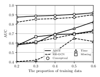
(a) ICEWS 14

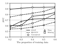
(b) ICEWS 05-15

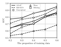
(c) YAGO 11k

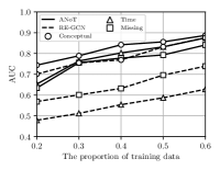
(d) GDELT

Figure 5. Performance of ANoT and RE-GCN when different proportions of offline preserved knowledge are used to construct the optimal rule graph. Concept, time, and missing respectively refer to conceptual errors, time errors, and missing errors.

Table 3. Performance comparison of ANoT and its variants.

	Dataset	ICEWS 14			ICEWS 05-15			YAGO 11k			GDELT
Variants	Anomaly	Precision	$F_{\beta}$ score	AUC	Precision	$F_{\beta}$ score	AUC	Precision	$F_{\beta}$ score	AUC	Precision	$F_{\beta}$ score	AUC
	Conceptual errors	0.657	0.680	0.886	0.714	0.736	0.875	0.798	0.807	0.926	0.873	0.796	0.842
Remove category aggregations	Time errors	0.618	0.602	0.758	0.577	0.489	0.676	0.494	0.541	0.846	0.688	0.741	0.833
	Missing errors	0.784	0.667	0.681	0.856	0.743	0.801	0.965	0.903	0.842	0.656	0.618	0.799
	Conceptual errors	0.784	0.781	0.912	0.844	0.810	0.927	0.805	0.815	0.944	0.901	0.817	0.851
Remove updater module	Time errors	0.551	0.585	0.796	0.530	0.519	0.697	0.438	0.494	0.807	0.670	0.712	0.812
	Missing errors	0.801	0.667	0.689	0.875	0.778	0.807	0.951	0.891	0.840	0.644	0.678	0.809
Remove triadic occurring rule edges	Time errors	0.614	0.646	0.812	0.572	0.498	0.685	0.495	0.552	0.846	0.687	0.752	0.844
	Missing errors	0.789	0.693	0.718	0.876	0.792	0.816	0.965	0.912	0.852	0.665	0.635	0.806
Remove recursive strategy	Time errors	0.618	0.634	0.815	0.581	0.522	0.703	0.494	0.550	0.831	0.698	0.761	0.854
	Missing errors	0.792	0.692	0.714	0.882	0.786	0.814	0.962	0.915	0.850	0.670	0.679	0.818
	Conceptual errors	0.784	0.781	0.912	0.844	0.810	0.927	0.805	0.815	0.944	0.901	0.817	0.851
Ranking rules and rule edges only by $|\mathcal{A}^{\mathcal{G}}|\downarrow$	Time errors	0.551	0.585	0.796	0.530	0.519	0.697	0.438	0.494	0.807	0.670	0.712	0.812
	Missing errors	0.801	0.667	0.689	0.875	0.778	0.807	0.951	0.891	0.840	0.644	0.678	0.809
	Conceptual errors	0.781	0.769	0.901	0.838	0.809	0.931	0.814	0.832	0.941	0.915	0.826	0.877
Replace $|\mathcal{A}_{v}^{\mathcal{G}}|$ as 1 when deriving scores	Time errors	0.493	0.448	0.603	0.332	0.375	0.646	0.478	0.529	0.810	0.584	0.632	0.701
	Missing errors	0.820	0.584	0.693	0.859	0.732	0.798	0.976	0.873	0.857	0.636	0.642	0.788
	Conceptual errors	0.789	0.792	0.921	0.847	0.815	0.933	0.829	0.841	0.952	0.936	0.835	0.887
Original	Time errors	0.639	0.661	0.825	0.601	0.526	0.729	0.524	0.579	0.863	0.710	0.786	0.875
	Missing errors	0.822	0.705	0.730	0.894	0.797	0.834	0.988	0.933	0.867	0.683	0.696	0.841

5.4. RQ2: Effect of Each Component

Ablation study. As shown in Table 3, removing category aggregations will result in a degradation in performance. This is because first, small relation combinations cannot reflect fine-grained categories; furthermore, aggregation strategies can summarize redundant categories and thus help to alleviate the effect of data noises. Removing the updater module will result in the model failing to adapt to the new knowledge, thus degrading the performance, especially in detecting time errors. This is because temporal patterns change more frequently and thus require timely updating. Figure 6 shows the long-time detection performance, particularly for unseen knowledge, with and without the updater module. We can see that the updater can constantly enhance performance across different timestamps, demonstrating its effectiveness in handling new emerging knowledge and patterns. Since triadic rule edges and recursive strategies only affect the temporal scoring, only results of time errors and missing errors are reported. We can see that they both contribute to the detection performance, demonstrating the effectiveness of triadic rule edges in describing knowledge-occurring patterns and recursive strategies in supporting more stable scoring.

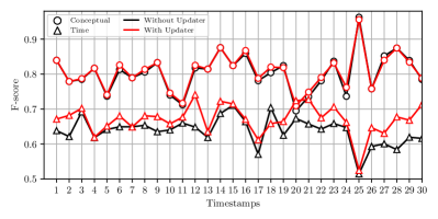
(a) ICEWS 14

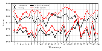
(b) GDELT

Figure 6. Inductive detection performance of ANoT across different timestamps on the ICEWS 14 and GDELT datasets.

Comparison with variants. We further analyze the effectiveness of our ranking strategy. As shown in Table 3, when we rank the atomic rules and rule edges only by the number of correct assertions $|\mathcal{A}^{\mathcal{G}}|$, the performance of all anomaly types degrades. This is because the rules and rule edges with larger $|\mathcal{A}^{\mathcal{G}}|$ are not necessarily helpful in improving the expressiveness of the model and thus may introduce low-expressive rules and edges. When we only use the number of mapped rules and rule edges to derive scores, the performance degrades especially for the time errors. This shows the effectiveness of considering different expression powers.

Effects of the number of recursive steps $K$. As shown in Figure 7, when $K$ increases from 1 to 2, the detection performances on all four datasets improve, which demonstrates the effectiveness of our recursive strategy in achieving more accurate scoring. However, when $K$ continues to increase, the performance will gradually degrade. This is because the more steps required by a reachable node, the more uncertain it can be evidence for new knowledge. Thus, a too large $K$ will bring much noise during scoring.

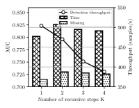
(a) ICEWS 14

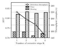
(b) ICEWS 05-15

(c) YAGO 11k

(d) GDELT

Figure 7. Performance and detection throughput of ANoT under the different settings of the number of recursive steps $K$.

Effects of the length of timespan $L$. As shown in Figure 8, different datasets require different $L$ to get the best performance. We notice that the best $L$ is largely related to the size of each dataset (e.g., 200 for ICEWS 14 and 2000 for ICEWS 05-15). This may be because a larger TKG requires a larger $L$ to extract long-range patterns. The YAGO 11k dataset requires a small $L$ since its granularity is a month but other datasets are day or minute.

(a) ICEWS 14

(b) ICEWS 05-15

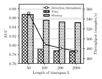
(c) YAGO 11k

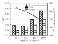
(d) GDELT

Figure 8. Performance and detection throughput of ANoT under the different settings of the timespan length $L$.

Effects of the number of entity categories $k$. As shown in Figure 9, two ICEWS datasets get the nearly best performance when $k$ is 3, and keep stable when $k$ continues to be larger. This demonstrates that our category function can effectively extract the properties shared by different entities. The YAGO 11k dataset has a smaller number of relations which limits the expression power of each relation combination and thus requires more categories.

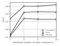
(a) ICEWS 14

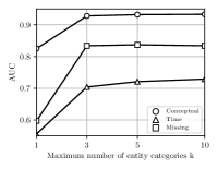
(b) ICEWS 05-15

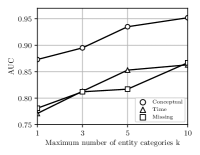
(c) YAGO 11k

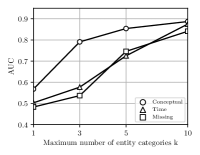
(d) GDELT

Figure 9. Performance of ANoT under the different settings of the number of entity categories $k$.

5.5. RQ3: Efficiency Analysis

Detection efficiency. As shown in Figure 7, we analyze how the recursive steps $K$ affect the detection efficiency. With $K$ increases, the throughput of ANoT gradually decreases, but we can see that the best performance of ANoT does not rely on a large $K$. Therefore, a small $K$ can already achieve remarkable performance and acceptable efficiency. Furthermore, When $K$ increases, the reachable nodes increase exponentially but our throughput only decreases linearly, which also shows the effectiveness of our strategies.

In Figure 8, we analyze how the timespan $L$ affects the detection efficiency. We find that even though $L$ increases largely, the throughput only decreases linearly. This is because our ranking and selection strategies can avoid too many redundant rule edges being added to the rule graph, and thus reduce the searching time.

Table 4. Model building time, the sizes of the obtained optimal rule graph, and the proportions of explained facts under different settings of category number $K$.

	ICEWS 14				ICEWS 05-15				YAGO 11k				GDELT
Maximum number of entity categories $k$	1	3	5	10	1	3	5	10	1	3	5	10	1	3	5	10
Building time	49s	584s	629s	660s	773s	1,239s	1,577s	1,814s	44s	50s	65s	84s	1,160s	1,585s	2,081s	2,314s
Number of rule edges	97	6,349	5,428	5,064	3,751	9,688	11,053	11,384	92	76	66	63	87	20,223	27,847	30,106
Proportion of explained facts	0.132	0.766	0.767	0.767	0.165	0.788	0.853	0.874	0.716	0.909	0.908	0.907	0.170	0.896	0.894	0.894

Time consumption of building model. As shown in Table 4, the time consumption of building the optimal rule graph increases sub-linearly when the number of entity categories $k$ increases, which is acceptable in practice. The consumption of the YAGO 11k dataset is extremely small since it contains only a few relation categories, therefore the option spaces of the candidate rules and rule edges are smaller than other datasets. The size of the GDELT dataset is much larger than other datasets but our ANoT can still handle it within one hour (baselines need over 100 epochs to train while each epoch needs nearly 3 minutes), showing our efficiency.

Size of the optimal rule graph. We further analyze the size of the obtained optimal rule graph in Table 4. As the number of entity categories $k$ continuously increases, the number of rule edges becomes stable or even slightly decreases, meaning that the construction of the optimal rule graph is robust to the entity categories. The decrease may be because a larger number of entity categories can expand the number of candidate rules and rule edges, and thus help ANoT to find more powerful patterns. We further find that as $k$ increases, the proportion of facts that can be explained gradually increases, which means improvements in the expression power of our rule graph. Combined with the results in Figure 9, the case with a high proportion of explained facts also has a high AUC in detection, showing the effectiveness of our selection strategies.

Table 5. Examples of the obtained entity categories and the entities that are assigned as these categories.

Entity category (relation combinations)	Described entities
host a visit — Express intent to provide military aid — Make statement — Express intent to change leadership	1. Xi Jinping, 2. Barack Obama, 3. Kim Jong-Un
Demand economic aid — Threaten with military force — Return or release person(s)	1. Naxalites group, 2. Rebel Group (Abu Sayyaf), 3. Combatant (Djibouti)
Died in — Was born in	1. China, 2. Japan, 3. United States 4. France
Has won prize	1. Nobel Peace Prize, 2. Fields Medal 3. Lasker Award
Reduce or break diplomatic relations — Bring a lawsuit against	1. Rights Activist (Ukraine), 2. Shamsul Islam Khan 3. Center for Reproductive Rights 4. Democratic Labor Party
Was born in — Created — Graduated from	1. Harry Weese, 2. I. M. Pei 3. Whit Stillman 4. Robert Ardrey

5.6. RQ4: Interpretability Analysis

Category interpretability. We select some representative entity categories and report their corresponding relation combinations and the entities that are assigned as these categories in Table 5. We can see that relations contained in one relation combination have related semantics, e.g., ‘Express intent to provide military aid’ and ‘Make statement’ are both political behaviors of leaders. Thus, relation combinations can imply entity categories. For example, ‘Was born in’ and ‘Created’ may imply artists, and ‘Express intent to provide military aid’ and ‘Make statement’ may imply presidents. The described entities of these categories also give evidence, e.g.,, ‘Barack Obama’ and ‘Kim Joung-Un’ are both presidents, and ‘Harry Weese’ and ‘I. M. Pei’ are both architects. These examples show the interpretability of our framework at the atomic rule level.

Table 6. Examples of rule edges in the obtained optimal rule graph.

Entity category (relation combinations)
(PERSON, Was born in, COUNTRY) $\rightarrow$ (PERSON, Died in, COUNTRY)
(PERSON, Created, PRODUCTS) $\rightarrow$ (PERSON, Owns, PRODUCTS)
(COUNTRY, Host a visit, PERSON) $\rightarrow$ (PERSON, Make a visit, COUNTRY)
(ORGANIZATION A, Cooperate, ORGANIZATION B) $\rightarrow$ (ORGANIZATION A, Consult, ORGANIZATION B)
(COUNTRY A, Accuse, PEOPLE), (COUNTRY A, Provide military aid, COUNTRY B) $\rightarrow$ (COUNTRY B, Accuse, PEOPLE)
(PERSON A, Was born in, COUNTRY), (PERSON A, Is married to, PERSON B) $\rightarrow$ (PERSON B, Was died in, COUNTRY)
(COUNTRY A, Investigate, COUNTRY B), (COUNTRY C, Criticize or denounce, COUNTRY B) $\rightarrow$ (COUNTRY A, Express intent to cooperate, COUNTRY C)
(COUNTRY A, Engage in negotiation, COUNTRY B), (COUNTRY C, Halt negotiations, COUNTRY B) $\rightarrow$ (COUNTRY A, Express intent to meet or negotiate, COUNTRY C)

Rule edge interpretability. In Table 6 we further select some representative rule edges to show the interpretability of our framework at the rule edge level. The chain-based rule edges extract some direct relevance between facts, such as ‘Create’ $\rightarrow$ ‘Owns’, while the triadic-based rule edges can extract more complex relevance, such as ‘Accuse’, ‘Provide military aid’ $\rightarrow$ ‘Accuse’ shows that countries with cooperation tend to have the same position. Based on these interpretable rules and rule edges, our ANoT can generate a set of human-readable prompts to describe what patterns a new knowledge comply and what patterns it violates.

5.7. RQ5: Generalization Analysis

Detection accuracy. Here we analyze the generalization ability of ANoT to the time-duration-based TKGs. We employ the most popular time-duration TKG benchmark Wikidata (Li et al., 2021) for evaluation. As shown in Table 7, ANoT can still outperform existing TKG embedding models, especially for the time errors, demonstrating its generalization ability, and the updater module can help our solution to adapt to time-duration-based pattern changes.

Effectiveness of adaption strategy. As illustrated in Figure 10(a), we can see that our strategy outperforms other simple strategies that can transfer time duration to timestamps, showing the effectiveness of our proposed four types of rule graphs in capturing various patterns in time-duration-based TKGs.

Effectiveness of different rule graphs. Figure 10(b) shows how four types of rule graphs contribute to the performance. We can see that all four types of rule graphs can describe a unique part of time-duration knowledge, showing their necessities. As the number of entity categories increases, each type of rule graph can describe more knowledge.

Table 7. $F_{\beta}$ score of ANoT and typical TKG embedding models on the time-duration-based TKG dataset Wikidata.

Model	Conceptual errors	Time errors	Missing errors
DE	0.849	0.560	0.869
TA	0.859	0.530	0.701
Timeplex	0.866	0.668	0.898
TNT	0.806	0.586	0.879
TELM	0.851	0.641	0.885
RE-GCN	0.858	0.697	0.903
ANoT (without updater)	0.961	0.687	0.951
ANoT	0.967	0.806	0.956

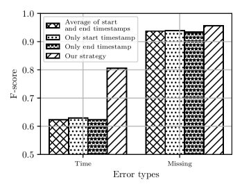
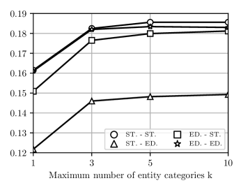
Figure 10. (a) Performance of different adaption strategies. (b) Proportions of facts explained by different rule graphs.

6. Conclusion

In this paper, we make the first attempt at strategies to summarize a temporal knowledge graph and first explore how to inductively detect anomalies in TKG. We propose a novel rule graph to map a TKG as a set of human-readable rules and rule edges. The rule graph allows us to flexibly infer complex patterns. Based on the rule graph, we propose an ANoT framework, which can efficiently detect anomaly knowledge by traversing the rule graph, and effectively adapt the rule graph to new knowledge. Extensive experimental results demonstrate the superiority of ANoT in accuracy, robustness, efficiency, and interpretability. In our future works, integrating our rule graph with graph learning methods is an interesting direction.

- (1)
- Aggarwal et al. (2011) Charu C. Aggarwal, Yuchen Zhao, and Philip S. Yu. 2011. Outlier detection in graph streams. In Proceedings of the 27th International Conference on Data Engineering, ICDE 2011, April 11-16, 2011, Hannover, Germany. 399–409.
- Belle et al. (2022) Rafaël Van Belle, Charles Van Damme, Hendrik Tytgat, and Jochen De Weerdt. 2022. Inductive Graph Representation Learning for fraud detection. Expert Syst. Appl. 193 (2022), 116463.
- Belth et al. (2020a) Caleb Belth, Xinyi Zheng, and Danai Koutra. 2020a. Mining Persistent Activity in Continually Evolving Networks. In KDD ’20: The 26th ACM SIGKDD Conference on Knowledge Discovery and Data Mining, Virtual Event, CA, USA, August 23-27, 2020. 934–944.
- Belth et al. (2020b) Caleb Belth, Xinyi Zheng, Jilles Vreeken, and Danai Koutra. 2020b. What is Normal, What is Strange, and What is Missing in a Knowledge Graph: Unified Characterization via Inductive Summarization. In WWW ’20: The Web Conference 2020, Taipei, Taiwan, April 20-24, 2020. 1115–1126.
- Bhatia et al. (2023) Siddharth Bhatia, Mohit Wadhwa, Kenji Kawaguchi, Neil Shah, Philip S. Yu, and Bryan Hooi. 2023. Sketch-Based Anomaly Detection in Streaming Graphs. In Proceedings of the 29th ACM SIGKDD Conference on Knowledge Discovery and Data Mining, KDD 2023, Long Beach, CA, USA, August 6-10, 2023. 93–104.
- Blasi et al. (2022) Maximilian Blasi, Manuel Freudenreich, Johannes Horvath, David Richerby, and Ansgar Scherp. 2022. Graph Summarization with Graph Neural Networks. CoRR abs/2203.05919 (2022).
- Cebiric et al. (2019) Sejla Cebiric, François Goasdoué, Haridimos Kondylakis, Dimitris Kotzinos, Ioana Manolescu, Georgia Troullinou, and Mussab Zneika. 2019. Summarizing semantic graphs: a survey. VLDB J. 28, 3 (2019), 295–327.
- Chang et al. (2021) Yen-Yu Chang, Pan Li, Rok Sosic, M. H. Afifi, Marco Schweighauser, and Jure Leskovec. 2021. F-FADE: Frequency Factorization for Anomaly Detection in Edge Streams. In WSDM ’21, The Fourteenth ACM International Conference on Web Search and Data Mining, Virtual Event, Israel, March 8-12, 2021. 589–597.
- Chen et al. (2009) Chen Chen, Cindy Xide Lin, Matt Fredrikson, Mihai Christodorescu, Xifeng Yan, and Jiawei Han. 2009. Mining Graph Patterns Efficiently via Randomized Summaries. Proc. VLDB Endow. 2, 1 (2009), 742–753.
- Dasgupta et al. (2018) Shib Sankar Dasgupta, Swayambhu Nath Ray, and Partha P. Talukdar. 2018. HyTE: Hyperplane-based Temporally aware Knowledge Graph Embedding. In Proceedings of the 2018 Conference on Empirical Methods in Natural Language Processing, Brussels, Belgium, October 31 - November 4, 2018. 2001–2011.
- Ding et al. (2020) Kaize Ding, Jundong Li, Nitin Agarwal, and Huan Liu. 2020. Inductive Anomaly Detection on Attributed Networks. In Proceedings of the Twenty-Ninth International Joint Conference on Artificial Intelligence, IJCAI 2020. 1288–1294.
- Eswaran and Faloutsos (2018) Dhivya Eswaran and Christos Faloutsos. 2018. SedanSpot: Detecting Anomalies in Edge Streams. In IEEE International Conference on Data Mining, ICDM 2018, Singapore, November 17-20, 2018. 953–958.
- Eswaran et al. (2018) Dhivya Eswaran, Christos Faloutsos, Sudipto Guha, and Nina Mishra. 2018. SpotLight: Detecting Anomalies in Streaming Graphs. In Proceedings of the 24th ACM SIGKDD International Conference on Knowledge Discovery & Data Mining, KDD 2018, London, UK, August 19-23, 2018. 1378–1386.
- Fan et al. (2022) Wenfei Fan, Ruochun Jin, Ping Lu, Chao Tian, and Ruiqi Xu. 2022. Towards Event Prediction in Temporal Graphs. Proc. VLDB Endow. 15, 9 (2022), 1861–1874.
- Fan et al. (2020) Yujie Fan, Yanfang Ye, Qian Peng, Jianfei Zhang, Yiming Zhang, Xusheng Xiao, Chuan Shi, Qi Xiong, Fudong Shao, and Liang Zhao. 2020. Metagraph Aggregated Heterogeneous Graph Neural Network for Illicit Traded Product Identification in Underground Market. In 20th IEEE International Conference on Data Mining, ICDM 2020, Sorrento, Italy, November 17-20, 2020. 132–141.
- Fang et al. (2023) Lanting Fang, Kaiyu Feng, Jie Gui, Shanshan Feng, and Aiqun Hu. 2023. Anonymous Edge Representation for Inductive Anomaly Detection in Dynamic Bipartite Graphs. Proc. VLDB Endow. 16, 5 (2023), 1154–1167.
- Galbrun (2022) Esther Galbrun. 2022. The minimum description length principle for pattern mining: a survey. Data Min. Knowl. Discov. 36, 5 (2022), 1679–1727.
- Gao et al. (2019) Junyang Gao, Xian Li, Yifan Ethan Xu, Bunyamin Sisman, Xin Luna Dong, and Jun Yang. 2019. Efficient Knowledge Graph Accuracy Evaluation. Proc. VLDB Endow. 12, 11 (2019), 1679–1691.
- García-Durán et al. (2018) Alberto García-Durán, Sebastijan Dumancic, and Mathias Niepert. 2018. Learning Sequence Encoders for Temporal Knowledge Graph Completion. In Proceedings of the 2018 Conference on Empirical Methods in Natural Language Processing, Brussels, Belgium, October 31 - November 4, 2018. 4816–4821.
- Goel et al. (2020) Rishab Goel, Seyed Mehran Kazemi, Marcus A. Brubaker, and Pascal Poupart. 2020. Diachronic Embedding for Temporal Knowledge Graph Completion. In The Thirty-Fourth AAAI Conference on Artificial Intelligence, AAAI 2020, The Thirty-Second Innovative Applications of Artificial Intelligence Conference, IAAI 2020, New York, NY, USA, February 7-12, 2020. 3988–3995.
- Guo et al. (2022) Xingzhi Guo, Baojian Zhou, and Steven Skiena. 2022. Subset Node Anomaly Tracking over Large Dynamic Graphs. In KDD ’22: The 28th ACM SIGKDD Conference on Knowledge Discovery and Data Mining, Washington, DC, USA, August 14 - 18, 2022. 475–485.
- Gupta et al. (2014) Pankaj Gupta, Venu Satuluri, Ajeet Grewal, Siva Gurumurthy, Volodymyr Zhabiuk, Quannan Li, and Jimmy Lin. 2014. Real-Time Twitter Recommendation: Online Motif Detection in Large Dynamic Graphs. Proc. VLDB Endow. 7, 13 (2014), 1379–1380.
- Hajiabadi et al. (2022) Mahdi Hajiabadi, Venkatesh Srinivasan, and Alex Thomo. 2022. Dynamic Graph Summarization: Optimal and Scalable. In IEEE International Conference on Big Data, Big Data 2022, Osaka, Japan, December 17-20, 2022. 545–554.
- Huffman (1952) David A. Huffman. 1952. A Method for the Construction of Minimum-Redundancy Codes. Proceedings of the IRE. 40, 9 (1952), 1098–1101.
- Jain et al. (2020) Prachi Jain, Sushant Rathi, Mausam, and Soumen Chakrabarti. 2020. Temporal Knowledge Base Completion: New Algorithms and Evaluation Protocols. In Proceedings of the 2020 Conference on Empirical Methods in Natural Language Processing, EMNLP 2020, Online, November 16-20, 2020. 3733–3747.
- Jia et al. (2019) Shengbin Jia, Yang Xiang, Xiaojun Chen, Kun Wang, and Shijia E. 2019. Triple Trustworthiness Measurement for Knowledge Graph. In The World Wide Web Conference, WWW 2019, San Francisco, CA, USA, May 13-17, 2019. 2865–2871.
- Jung et al. (2021) Jaehun Jung, Jinhong Jung, and U Kang. 2021. Learning to Walk across Time for Interpretable Temporal Knowledge Graph Completion. In KDD ’21: The 27th ACM SIGKDD Conference on Knowledge Discovery and Data Mining, Virtual Event, Singapore, August 14-18, 2021. 786–795.
- Lacroix et al. (2020) Timothée Lacroix, Guillaume Obozinski, and Nicolas Usunier. 2020. Tensor Decompositions for Temporal Knowledge Base Completion. In 8th International Conference on Learning Representations, ICLR 2020, Addis Ababa, Ethiopia, April 26-30, 2020.
- Li et al. (2021) Zixuan Li, Xiaolong Jin, Wei Li, Saiping Guan, Jiafeng Guo, Huawei Shen, Yuanzhuo Wang, and Xueqi Cheng. 2021. Temporal Knowledge Graph Reasoning Based on Evolutional Representation Learning. In SIGIR ’21: The 44th International ACM SIGIR Conference on Research and Development in Information Retrieval, Virtual Event, Canada, July 11-15, 2021. 408–417.
- Liu et al. (2023c) Huafeng Liu, Mingjie Zhou, Mingyang Song, Deqiang Ouyang, Yawen Li, Liping Jing, Jian Yu, and Michael K. Ng. 2023c. Learning Hierarchical Preferences for Recommendation with Mixture Intention Neural Stochastic Processes. IEEE Trans. Knowl. Data Eng. (2023). https://doi.org/10.1109/TKDE.2023.3348493
- Liu et al. (2023b) Kangzheng Liu, Feng Zhao, Guandong Xu, Xianzhi Wang, and Hai Jin. 2023b. RETIA: Relation-Entity Twin-Interact Aggregation for Temporal Knowledge Graph Extrapolation. In 39th IEEE International Conference on Data Engineering, ICDE 2023, Anaheim, CA, USA, April 3-7, 2023. 1761–1774.
- Liu et al. (2023a) Yixin Liu, Shirui Pan, Yu Guang Wang, Fei Xiong, Liang Wang, Qingfeng Chen, and Vincent Cheng-Siong Lee. 2023a. Anomaly Detection in Dynamic Graphs via Transformer. IEEE Trans. Knowl. Data Eng. 35, 12 (2023), 12081–12094.
- Maccioni and Abadi (2016) Antonio Maccioni and Daniel J. Abadi. 2016. Scalable Pattern Matching over Compressed Graphs via Dedensification. In Proceedings of the 22nd ACM SIGKDD International Conference on Knowledge Discovery and Data Mining, San Francisco, CA, USA, August 13-17, 2016. 1755–1764.
- Manzoor et al. (2016) Emaad A. Manzoor, Sadegh M. Milajerdi, and Leman Akoglu. 2016. Fast Memory-efficient Anomaly Detection in Streaming Heterogeneous Graphs. In Proceedings of the 22nd ACM SIGKDD International Conference on Knowledge Discovery and Data Mining, San Francisco, CA, USA, August 13-17, 2016. 1035–1044.
- Mondal and Deshpande (2012) Jayanta Mondal and Amol Deshpande. 2012. Managing large dynamic graphs efficiently. In Proceedings of the ACM SIGMOD International Conference on Management of Data, SIGMOD 2012, Scottsdale, AZ, USA, May 20-24, 2012. 145–156.
- Nasar et al. (2022) Zara Nasar, Syed Waqar Jaffry, and Muhammad Kamran Malik. 2022. Named Entity Recognition and Relation Extraction: State-of-the-Art. ACM Comput. Surv. 54, 1 (2022), 20:1–20:39.
- Park et al. (2022) Namyong Park, Fuchen Liu, Purvanshi Mehta, Dana Cristofor, Christos Faloutsos, and Yuxiao Dong. 2022. EvoKG: Jointly Modeling Event Time and Network Structure for Reasoning over Temporal Knowledge Graphs. In WSDM ’22: The Fifteenth ACM International Conference on Web Search and Data Mining, Virtual Event / Tempe, AZ, USA, February 21 - 25, 2022. 794–803.
- Pei et al. (2001) Jian Pei, Jiawei Han, Behzad Mortazavi-Asl, Helen Pinto, Qiming Chen, Umeshwar Dayal, and Meichun Hsu. 2001. PrefixSpan: Mining Sequential Patterns by Prefix-Projected Growth. In Proceedings of the 17th International Conference on Data Engineering, April 2-6, 2001, Heidelberg, Germany. 215–224.
- Ranshous et al. (2016) Stephen Ranshous, Steve Harenberg, Kshitij Sharma, and Nagiza F. Samatova. 2016. A Scalable Approach for Outlier Detection in Edge Streams Using Sketch-based Approximations. In Proceedings of the 2016 SIAM International Conference on Data Mining, Miami, Florida, USA, May 5-7, 2016. 189–197.
- Ren et al. (2023) Xin Ren, Luyi Bai, Qianwen Xiao, and Xiangxi Meng. 2023. Hierarchical Self-Attention Embedding for Temporal Knowledge Graph Completion. In Proceedings of the ACM Web Conference 2023, WWW 2023, Austin, TX, USA, 30 April 2023 - 4 May 2023. 2539–2547.
- Rissanen (1978) Jorma Rissanen. 1978. Modeling by shortest data description. Autom. 14, 5 (1978), 465–471.
- Rossi et al. (2022) Andrea Rossi, Donatella Firmani, Paolo Merialdo, and Tommaso Teofili. 2022. Kelpie: an Explainability Framework for Embedding-based Link Prediction Models. Proc. VLDB Endow. 15, 12 (2022), 3566–3569.
- Safavi et al. (2019) Tara Safavi, Caleb Belth, Lukas Faber, Davide Mottin, Emmanuel Müller, and Danai Koutra. 2019. Personalized Knowledge Graph Summarization: From the Cloud to Your Pocket. In 2019 IEEE International Conference on Data Mining, ICDM 2019, Beijing, China, November 8-11, 2019. 528–537.
- Salehi and Rashidi (2018) Mahsa Salehi and Lida Rashidi. 2018. A Survey on Anomaly detection in Evolving Data: [with Application to Forest Fire Risk Prediction]. SIGKDD Explor. 20, 1 (2018), 13–23.
- Shah et al. (2015) Neil Shah, Danai Koutra, Tianmin Zou, Brian Gallagher, and Christos Faloutsos. 2015. TimeCrunch: Interpretable Dynamic Graph Summarization. In Proceedings of the 21th ACM SIGKDD International Conference on Knowledge Discovery and Data Mining, Sydney, NSW, Australia, August 10-13, 2015. 1055–1064.
- Smirnova and Cudré-Mauroux (2019) Alisa Smirnova and Philippe Cudré-Mauroux. 2019. Relation Extraction Using Distant Supervision: A Survey. ACM Comput. Surv. 51, 5 (2019), 106:1–106:35.
- Sricharan and Das (2014) Kumar Sricharan and Kamalika Das. 2014. Localizing anomalous changes in time-evolving graphs. In International Conference on Management of Data, SIGMOD 2014, Snowbird, UT, USA, June 22-27, 2014. 1347–1358.
- Tang et al. (2019) Jizhi Tang, Yansong Feng, and Dongyan Zhao. 2019. Learning to Update Knowledge Graphs by Reading News. In Proceedings of the 2019 Conference on Empirical Methods in Natural Language Processing and the 9th International Joint Conference on Natural Language Processing, EMNLP-IJCNLP 2019, Hong Kong, China, November 3-7, 2019. 2632–2641.
- Trouillon et al. (2017) Théo Trouillon, Christopher R. Dance, Éric Gaussier, Johannes Welbl, Sebastian Riedel, and Guillaume Bouchard. 2017. Knowledge Graph Completion via Complex Tensor Factorization. J. Mach. Learn. Res. 18 (2017), 130:1–130:38.
- Wang et al. (2023) Jiapu Wang, Boyue Wang, Meikang Qiu, Shirui Pan, Bo Xiong, Heng Liu, Linhao Luo, Tengfei Liu, Yongli Hu, Baocai Yin, and Wen Gao. 2023. A Survey on Temporal Knowledge Graph Completion: Taxonomy, Progress, and Prospects. CoRR abs/2308.02457 (2023).
- Wang et al. (2020) Pei Wang, Junqi Wang, Pushpi Paranamana, and Patrick Shafto. 2020. A mathematical theory of cooperative communication. In Advances in Neural Information Processing Systems 33: Annual Conference on Neural Information Processing Systems 2020, NeurIPS 2020, December 6-12, 2020, virtual.
- Wu et al. (2020) Jiapeng Wu, Meng Cao, Jackie Chi Kit Cheung, and William L. Hamilton. 2020. TeMP: Temporal Message Passing for Temporal Knowledge Graph Completion. In Proceedings of the 2020 Conference on Empirical Methods in Natural Language Processing, EMNLP 2020, Online, November 16-20, 2020. 5730–5746.
- Wu et al. (2013) Yinghui Wu, Shengqi Yang, Mudhakar Srivatsa, Arun Iyengar, and Xifeng Yan. 2013. Summarizing Answer Graphs Induced by Keyword Queries. Proc. VLDB Endow. 6, 14 (2013), 1774–1785.
- Xu et al. (2021) Chengjin Xu, Yung-Yu Chen, Mojtaba Nayyeri, and Jens Lehmann. 2021. Temporal Knowledge Graph Completion using a Linear Temporal Regularizer and Multivector Embeddings. In NAACL-HLT. 2569–2578.
- Xu et al. (2020a) Chenjin Xu, Mojtaba Nayyeri, Fouad Alkhoury, Hamed Shariat Yazdi, and Jens Lehmann. 2020a. Temporal Knowledge Graph Completion Based on Time Series Gaussian Embedding. In The Semantic Web - ISWC 2020 - 19th International Semantic Web Conference, Athens, Greece, November 2-6, 2020, Proceedings, Part I. 654–671.
- Xu et al. (2020b) Chengjin Xu, Mojtaba Nayyeri, Fouad Alkhoury, Hamed Shariat Yazdi, and Jens Lehmann. 2020b. TeRo: A Time-aware Knowledge Graph Embedding via Temporal Rotation. In Proceedings of the 28th International Conference on Computational Linguistics, COLING 2020, Barcelona, Spain (Online), December 8-13, 2020. 1583–1593.
- Yang et al. (2024) Jinfa Yang, Xianghua Ying, Yongjie Shi, and Bowei Xing. 2024. Tensor decompositions for temporal knowledge graph completion with time perspective. Expert Syst. Appl. 237, Part A (2024), 121267.
- You et al. (2020) Jiaxuan You, Xiaobai Ma, Daisy Yi Ding, Mykel J. Kochenderfer, and Jure Leskovec. 2020. Handling Missing Data with Graph Representation Learning. In Advances in Neural Information Processing Systems 33: Annual Conference on Neural Information Processing Systems 2020, NeurIPS 2020, December 6-12, 2020, virtual.
- Yu et al. (2018) Wenchao Yu, Wei Cheng, Charu C. Aggarwal, Kai Zhang, Haifeng Chen, and Wei Wang. 2018. NetWalk: A Flexible Deep Embedding Approach for Anomaly Detection in Dynamic Networks. In Proceedings of the 24th ACM SIGKDD International Conference on Knowledge Discovery & Data Mining, KDD 2018, London, UK, August 19-23, 2018. 2672–2681.
- Zhang et al. (2024) Fu Zhang, Hongzhi Chen, Yuzhe Shi, Jingwei Cheng, and Jinghao Lin. 2024. Joint framework for tensor decomposition-based temporal knowledge graph completion. Inf. Sci. 654 (2024), 119853.
- Zhang et al. (2022) Jiasheng Zhang, Shuang Liang, Yongpan Sheng, and Jie Shao. 2022. Temporal knowledge graph representation learning with local and global evolutions. Knowl. Based Syst. 251 (2022), 109234.
- Zheng et al. (2019) Li Zheng, Zhenpeng Li, Jian Li, Zhao Li, and Jun Gao. 2019. AddGraph: Anomaly Detection in Dynamic Graph Using Attention-based Temporal GCN. In Proceedings of the Twenty-Eighth International Joint Conference on Artificial Intelligence, IJCAI 2019, Macao, China, August 10-16, 2019. 4419–4425.
- Zheng et al. (2018) Weiguo Zheng, Jeffrey Xu Yu, Lei Zou, and Hong Cheng. 2018. Question Answering Over Knowledge Graphs: Question Understanding Via Template Decomposition. Proc. VLDB Endow. 11, 11 (2018), 1373–1386.
- Zhu et al. (2023) Xinyi Zhu, Liping Wang, Hao Xin, Xiaohan Wang, Zhifeng Jia, Jiyao Wang, Chunming Ma, and Yuxiang Zengt. 2023. T-FinKB: A Platform of Temporal Financial Knowledge Base Construction. In 39th IEEE International Conference on Data Engineering, ICDE 2023, Anaheim, CA, USA, April 3-7, 2023. 3671–3674.