A Pride of Satellites in the Constellation Leo? Discovery of the Leo VI Milky Way Satellite Ultra-Faint Dwarf Galaxy with DELVE Early Data Release 3

Abstract

We report the discovery and spectroscopic confirmation of an ultra-faint Milky Way (MW) satellite in the constellation of Leo. This system was discovered as a spatial overdensity of resolved stars observed with Dark Energy Camera (DECam) data from an early version of the third data release of the DECam Local Volume Exploration survey (DELVE EDR3). The low luminosity ($M_{V}=-3.56_{-0.37}^{+0.47}$ ; $L_{V}=2300_{-800}^{+1000}L_{\odot}$), large size ($r_{1/2}=90_{-30}^{+30}$ pc), and large heliocentric distance (${D=111_{-4}^{+7}}$  kpc) are all consistent with the population of ultra-faint dwarf galaxies (UFDs). Using Keck/DEIMOS observations of the system, we were able to spectroscopically confirm 11 member stars, while measuring a tentative mass to light ratio of $1000_{-700}^{+1900}M_{\odot}/L_{\odot}$ and a non-zero metallicity dispersion of $\sigma_{[\rm Fe/H]}=0.33_{-0.14}^{+0.19}$, further confirming Leo VI’s identity as an UFD. While the system has a highly elliptical shape, $\epsilon=0.54_{-0.29}^{+0.19}$, we do not find any evidence that it is tidally disrupting. Moreover, despite the apparent on-sky proximity of Leo VI to members of the proposed Crater-Leo infall group, its smaller heliocentric distance and inconsistent position in energy-angular momentum space make it unlikely that Leo VI is part of the proposed infall group.

FERMILAB-PUB-24-0358-LDRD-PPD

1 Introduction

Ultra-faint dwarf galaxies (UFDs) are among the oldest, faintest ($M_{V}\gtrsim-7.7$; $L_{V}\lesssim 10^{5}L_{\odot}$), most metal-poor ($\mbox{[Fe/H]}\lesssim-2$), and most dark-matter-dominated ($M_{\odot}/L_{\odot}>100$) stellar systems known (Simon, 2019). UFDs were first discovered in the Sloan Digital Sky Survey (SDSS; Willman et al., 2005a, b) following the advent of CCD-based digital sky surveys. Subsequently, more recent surveys such as the Pan-STARRS-1 (Chambers et al., 2016), the Dark Energy Survey (DES: Dark Energy Survey Collaboration et al., 2016), and the DECam Local Volume Exploration Survey (DELVE; Drlica-Wagner et al., 2021) have drastically expanded the known population of these faint resolved systems around the MW to more than 60 systems (e.g., Laevens et al., 2015; Koposov et al., 2015; Bechtol et al., 2015; Drlica-Wagner et al., 2015, 2020; Mau et al., 2020; Cerny et al., 2023a).

The high dark matter content of UFDs makes them excellent laboratories for understanding the nature of dark matter. For example, the luminosity function of UFDs and their density profiles depend sensitively on the dark matter particle mass, thermal history, and self-interaction cross section (e.g., Lovell et al., 2014; Rocha et al., 2013; Kaplinghat et al., 2016; Bullock & Boylan-Kolchin, 2017). Their internal dynamics are also sensitive to weak heating effects from the dark matter halo, allowing for potentially measurable effects on their stellar components (Brandt, 2016; Peñarrubia et al., 2016). UFDs are also excellent targets to search for Standard Model products coming from dark matter annihilation or decay due to their proximity, high dark matter content, and lack of high-energy astrophysical backgrounds (e.g., Ackermann et al., 2015; Bonnivard et al., 2015; Geringer-Sameth et al., 2015b; McDaniel et al., 2023; Boddy et al., 2024). Furthermore, the study of individual UFDs can yield insights into the processes of satellite accretion and tidal disruption around MW mass host galaxies. Due to their low luminosities, most of the UFD systems discovered thus far are resolved satellites of the MW and other nearby galaxies in the Local Volume (see Simon 2019 and the reference therein.)

In this paper, we present the discovery and confirmation of the UFD Leo VI, a low-luminosity, metal-poor MW satellite located at a heliocentric distance of $\sim$110 kpc. The paper also acts as an reference for the DELVE EDR3 dataset used to discover the system, which we describe in detail in Section 2. We use Section 3 to describe the matched filter search methods used to discover Leo VI in DELVE EDR3 and Section 4 to present system’s morphological properties obtained from follow-up DECam observations. In Section 5, we describe the line-of-sight velocity and metallicity measurements of the member stars of Leo VI obtained through follow-up Keck/DEIMOS data. We then discuss whether Leo VI could be tidally disrupting as well as its potential associations with other Local Group systems in Section 6 and summarize our results in Section 7.

2 DELVE Early Data Release 3

DELVE is an ongoing observing program that uses DECam (Flaugher et al., 2015) on the 4-m Blanco Telescope at the Cerro Tololo Inter-American Observatory (CTIO) in Chile to contiguously image the high Galactic latitude southern sky in the $g$, $r$, $i$, and $z$ bands (Drlica-Wagner et al., 2021, 2022). To date, DELVE has been allocated more than 150 nights to pursue three observational programs dedicated to studying ultra-faint satellite galaxies around the MW (DELVE–WIDE), the Magellanic Clouds (DELVE–MC), and Magellanic analogs in the Local Volume (DELVE–DEEP). New DECam observations and public archival DECam data are self-consistently processed using the DES Data Management pipeline (DESDM: Morganson et al., 2018).

The forthcoming DELVE third data release combines exposures from DELVE with other public DECam programs such as DES and the DECam Legacy Survey (DECaLS: Dey et al., 2019). Compared to the previous DELVE data release, the exposures were coadded to improve the depth and precision of photometric measurements. In this analysis, we use an object catalog from DELVE EDR3 which is an early internal version of the third DELVE data release containing only exposures in the Northern Galactic cap ($b>10^{\circ}$). While DELVE EDR3 is an internal data release, the full DELVE DR3 follows the same processing procedure and will be made publicly available in the future.

The DELVE EDR3 data were self-consistently processed using the DESDM pipeline in the context of the DECam All Data Everywhere (DECADE) program at the National Center for Supercomputing Applications (NCSA). The configuration of the DESDM image detrending and coaddition pipeline closely follows the pipeline used to produce DES DR2 (Abbott et al., 2021). We briefly summarize key aspects of the DESDM pipeline used to produce DELVE EDR3 here.

Processing of individual DECam exposures was performed following the “Final Cut” pipeline described in Morganson et al. (2018). All exposures go through a preprocessing step, which includes crosstalk and overscan correction as well as bad pixel masking for each DECam CCD. In addition, we correct for the CCD nonlinearity with CCD-dependent lookup tables that convert the observed flux to the fitted model (Bernstein et al., 2017). To account for the “brighter-fatter effect”, we use a CCD-dependent kernel derived from early DECam data by Gruen et al. (2015). We then apply flat field corrections using the raw, bias, dome flats, amplifier-specific conversion, and the non-linear correction to each CCD. For the bias and dome flat images, we used a set of “supercals” assembled for DES by combining bias and flats taken over several nights (see Section 3.2 of Morganson et al., 2018). The bias, dome flat images, and other image calibration data products were used corresponding to the nearest DES observing epoch.

At the time of observations, a world coordinate system (WCS) was added to the image using the optical axis read from the telescope encoders and a fixed distortion map derived from the star flats. The WCS is then updated with an initial single-exposure astrometric solution calculated using SCAMP (Bertin, 2006), with Gaia DR2 (Gaia Collaboration et al., 2018) used as the reference catalog without proper motion corrections. The single-epoch astrometric accuracy is found to have a minimal value of $\approx$ 20 mas for DECam data taken close to the Gaia 2015.5 epoch; however, it is found to increase before and after that date (Abbott et al., 2021).

To remove image artifacts, we mask the saturated pixels caused by bright stars, and the associated charge overflow in both the readout direction (“bleed trails”) and the CCD serial register (“edge bleeds”). We also perform cosmic ray masking using a modified version of the algorithm developed for the Legacy Survey of Space and Time (LSST; Jurić et al., 2017) and a satellite streak mask using an algorithm based on the Hough Transform (Morganson et al., 2018).

To account for the sky background light, we also fit and subtract the sky background from the whole DECam exposure using seasonally averaged PCA components and divide the image by the star flat (Bernstein et al., 2017). The sky background model is produced from the raw bias, dome flat, and nightly star flat images and quantifies the differences between the dome flat and the response to astronomical flux. The point spread function (PSF) for each CCD image is obtained using PSFEx (Bertin, 2011). Finally, the source catalog for each individual CCD image is then produced using SourceExtractor (Bertin & Arnouts, 1996) with a detection threshold of $\sim 3\sigma$ (Abbott et al., 2021).

The DELVE EDR3 coadded images were assembled from a subset of DECam exposures that were publicly available as of 2022 December 5. The coadd input exposures were selected to reside in the northern Galactic cap ($b>10\arcdeg$) and to have an exposure time between 30 and 350 seconds. Furthermore, we require that the images have a PSF full width at half maximum (FWHM) value of between 0” $<$ FWHM $<$ 1.5” and that all exposures have an effective exposure time scale factor $t_{\rm eff}>0.2$, where $t_{\rm eff}$ is calculated based on nominal values of the PSF FWHM, sky brightness, and transparency as described in Neilsen et al. (2016). We also require that the input exposures have a good astrometric solution when matched to Gaia DR2. This is achieved by requiring $>$ 250 astrometric matches, $\chi^{2}_{\rm astrom}<180$, and an average difference of $\Delta_{\rm astrom}<100$ mas. As with Drlica-Wagner et al. (2022), to remove exposures with excess electronic noise or poor sky background estimation resulting in many spurious object detections, we also require that the number of objects detected in each exposure is less than the empirically determined limit of $7.5\times 10^{5}$. To improve the quality of the input exposures going into the coadding process, we further remove exposures that were identified as having suspect sky subtraction and/or astrometric fits based on selection criteria developed for DES (Abbott et al., 2021).

Since the public DECam exposures were taken for a wide variety of science purposes with different exposure times and filter distributions, there are variations in survey depth and filter coverage across the footprint. Therefore, to improve the uniformity of the dataset, we select exposures to homogenize the cumulative effective exposure time across the DELVE footprint. This homogenization is performed by iteratively adding exposures to the coadd input list, starting with the exposure with the highest effective exposure time ($t_{\rm eff}\times t_{\rm exp}$). Exposures are iteratively added to the input list in order of effective exposure time unless $>95\%$ of the exposure area is already covered by 15 or more exposures in the same band. The homogenization process removed 11% of all the exposures and resulted in the standard deviation of the effective exposure time ($t_{\rm eff}\times t_{\rm exp}$) across the survey area in $g$-band to drop from 1773s to 630s. This selection results in the selection of 61,425 exposures in the $g,r,i,z$ bands in the northern Galactic cap ($b>10\arcdeg$).

Individual CCD images are further checked for quality by automated algorithms and visual inspection (e.g., looking for issues similar to those described in Melchior et al., 2016). In particular, we identify images that are strongly affected by optical ghosting (Kent, 2013), electronic noise variations, telescope motion (e.g., bad tracking, earthquakes, etc.), airplanes in the field of view, and other similar issues that lead to poor data quality. These quality checks are performed at both the exposure and individual CCD level, and the individual CCD images that contain artifacts are removed from the coadd input list. In total, 10,796 out of 6,440,109 CCD images were removed by this inspection.

Photometric calibration was performed by matching to the ATLAS RefCat2 reference catalog (Tonry et al., 2018). ATLAS RefCat2 is an all-sky catalog that combines several surveys (i.e., Gaia, PS1, SkyMapper, etc.). For the purposes of DELVE calibration, we utilize the PS1 measurements in the north (${\rm Dec.}>-30\arcdeg$) and SkyMapper measurements in the south (${\rm Dec.}<-30\arcdeg$). The calibration followed the procedure described for DELVE DR2 (Drlica-Wagner et al., 2022), but with an updated transformation procedure that finds the offsets required to convert the magnitudes for sources in different color bins and makes an interpolation for the intermediate color values (Thanjavur et al., 2021). Separate interpolations were derived for the northern (PS1) and southern (SkyMapper) parts of the sky by matching the DES DR2 WAVG_MAG_PSF magnitudes to the corresponding ATLAS RefCat2 magnitudes to remove the $\sim$5 mmag offset detected in DELVE DR2 (Drlica-Wagner et al., 2022). Photometric zeropoints for each DECam CCD were obtained by performing a $1\arcsec$ match between the DECam Final Cut catalogs and ATLAS RefCat2. The ATLAS RefCat2 measurements are transformed into the DECam system using interpolations, and the zeropoint is derived from the median offset required to match the ATLAS RefCat2 values. We repeated the calibration process for each CCD three times, with each iteration removing outlier sources where the magnitude difference between the zeropoint-calibrated sources and ATLAS RefCat2 values is $>3\sigma$ from the mean. The relative photometric uncertainty was validated through comparison to Gaia EDR3 using transformation equations derived for DES DR2 (Abbott et al., 2021) and by measurements of the width of the stellar locus following the procedures described in Drlica-Wagner et al. (2022). Calibrated single-epoch sources were found to agree with Gaia magnitudes with a scatter of $\pm$4.2 mmag (estimated using half the width of the 68% containment).

The image coaddition process follows that described in Section 6 of Morganson et al. (2018). Coadded images are built in distinct rectangular tiles that have dimensions of $0.71\times 0.71$ deg covered by 10,000 pixels with a pixel scale of 0.263 arcsec. Coadd images were constructed for tiles that had at least partial coverage in all four bands ($g$,$r$,$i$,$z$). To minimize the FWHM of the coadded PSF due to astrometric offsets between input exposures, we recompute a global astrometric solution for all CCD images provided as input to each coadd tile. For each tile, we use SCAMP (Bertin, 2006) to perform an astrometric refinement by simultaneously solving for the astrometry using the Final Cut catalogs for each input CCD and Gaia DR2 as an external reference catalog. Using this process, the DES pipeline obtained residuals from the simultaneous astrometric fit with a standard deviation of $\sim$27 mas (Abbott et al., 2021). We then use SWARP (Bertin et al., 2002) to resample the input images and produce the final coadd images for all four bands ($g,r,i,z$). In addition to the individual bands, we also produce a detection image, which is a coadd of the $r+i+z$ images using the COMBINE$\_$TYPE=AVERAGE procedure in SWARP (Abbott et al., 2021).

Object detection is performed on the $r+i+z$ detection coadd image using SourceExtractor following the procedure described for DES DR2 (Abbott et al., 2021). Objects are detected when contiguous groups of 4 or more pixels exceed a threshold of 1.5$\sigma$, which has been found to correspond to a source detection threshold of $\sim 5\sigma$ (Abbott et al., 2021). Initial photometric measurement is performed with SourceExtractor in “dual image mode,” using the detection image and the band of interest. Object astrometry comes from the windowed positions derived by SourceExtractor on the coadd images. The DELVE EDR3 footprint contains 6,895 coadd tiles, which covers 7,737 deg² with a median limiting magnitude of $g\sim 24.1$, $r\sim 23.6$, $i\sim 23.2$, $z\sim 22.5$ (estimated at ${\rm S/N}=10$ in 2$\arcsec$ aperture from survey property maps derived from the single-epoch images that go into the coadds). For comparison, the median limiting magnitude of DES DR2 assessed at the same S/N with the same technique is $g\sim 24.7$, $r\sim 24.4$, $i\sim 23.8$, $z\sim 23.1$ (Abbott et al., 2021). In contrast, the DELVE DR2 limiting PSF magnitude at S/N =10 is $g\sim 23.5$, $r\sim 23.1$, $i\sim 22.7$, $z\sim 22.1$ (Drlica-Wagner et al., 2022).

We perform multi-epoch photometric fitting following the procedures developed for cosmology analyses using the DES Y3 DEEP fields (e.g., Hartley et al., 2022; Everett et al., 2022). We first create multi-epoch data structures (MEDS; Jarvis et al., 2016; Zuntz et al., 2018) consisting of cutouts centered on each object detected in the coadd images. The dimensions of the MEDS range in size from $32\times 32$ to $256\times 256$ pixels, and they are comprised of the individual constituent images that went into the coadd at the location of each detected object. We perform multi-band, multi-epoch fitting using the fitvd tool (Hartley et al., 2022), which is built on top of the core functionality of ngmix (Sheldon, 2014). We perform PSF model fits and bulge + disk model fits (BDF) while masking neighboring sources (i.e., a “single-object fit”, SOF, in the DES nomenclature). The PSF model fits are obtained by fitting the amplitude of the individual-epoch PSF models, while the BDF fits consist of fitting a galaxy model with bulge and disk components that are Sérsic profiles with fixed indices of $n=4$ and $n=1$, respectively. To reduce the degeneracies in the parameters, the relative effective radii of the bulge and disk components in the BDF fits are fixed to unity. The magnitudes referenced in this paper are from the fitvd PSF fit, which has been found to provide the best photometry for point-like sources (Abbott et al., 2021).

We append several “value added” columns to the catalogs. Due to the increased depth of the DELVE EDR3 catalog relative to DELVE DR2 and the rapidly rising number density of faint background galaxies, the effects of star–galaxy misclassification can become more prominent in searches for resolved stellar systems. We perform star–galaxy separation using the sizes and signal-to-noise ratios of the sources measured by the multi-epoch fitvd fit following a classification procedure developed for DES Y6 (Bechtol et al., in prep). The classifier assigns an integer object class (ranging from 0 being likely stars to 4 being likely galaxies) to each source. Using DES data, a relatively pure sample of stars with $0\leq\texttt{EXT\_FITVD}\leq 1$ has been found to have a stellar efficiency (true positive rate) of 90% with galaxy contamination (false discovery rate) of 10% when integrating over a magnitude range $19\leq i\leq 23.5$, while a more complete stellar sample selected with $0\leq\texttt{EXT\_FITVD}\leq{3}$ has a stellar efficiency of 96% with galaxy contamination of 27% over the same magnitude range. The relative stellar efficiency (and galaxy contamination) of the classification procedure starts to drop (increase) strongly with magnitude starting at $i\sim$23.

To calculate the extinction due to interstellar dust, we first obtain the value of $E(B-V)$ by performing a bi-linear interpolation to the Schlegel et al. (1998) maps at the location of each source in the catalog. The reddening correction for each band is then calculated using the fiducial interstellar extinction coefficients from DES DR2 such that $A_{b}=R_{b}\times E(B-V)$ where $R_{g}=3.186$, $R_{r}=2.140$, $R_{i}=1.569$, and $R_{z}=1.196$ (Abbott et al., 2021). As described in Abbott et al. (2021), these coefficients include a renormalization of the $E(B-V)$ extinction values ($N=0.78$) as suggested by Schlafly et al. (2010) and Schlafly & Finkbeiner (2011) so that they can be used directly with the $E(B-V)$ values from the Schlegel et al. (1998) map. In this paper, we denote extinction-corrected magnitudes with the subscript “0”.

3 The Discovery of Leo VI

Figure 1: Diagnostic plots for Leo VI constructed with the deeper follow-up DECam photometric data. Left: Smoothed isochrone-filtered spatial density of stars in the region around the Leo VI. The system appears as a significant overdensity against a relatively constant background. Center Left: Smoothed isochrone-filtered spatial density of galaxies. Center Right: Color–magnitude diagram (CMD) of stars that are within 4′ of the centroid of the system. Right: Color-magnitude Hess diagram of the foreground stars within 4′ of the centroid of Leo VI minus the background stars in a concentric annulus with radius from 12′ to 12.65′. We use the ugali best-fit old ($\tau\sim$13.3 Gyr), metal poor (Z = 0.0001, [Fe/H] $\sim-2.2$) PARSEC isochrone with distance modulus of $(m-M)_{0}=20.2$ for this figure.

We search for resolved stellar systems in the DELVE EDR3 catalog using the simple matched-filter search algorithm (Bechtol et al., 2015; Drlica-Wagner et al., 2020). This algorithm has been successfully used to discover more than twenty MW satellites to date (e.g. Bechtol et al., 2015; Drlica-Wagner et al., 2015; Mau et al., 2020; Cerny et al., 2021a, 2023a). To parallelize the search across the DELVE EDR3 footprint, we first partition the catalog into HEALPix at the scale of NSIDE = 32 ($\approx$ 3.4 deg² per pixel). We then perform the search for each HEALPixelized catalog by combining the central catalog with catalogs from the 8 neighboring HEALPixels.

In our simple satellite search, we select stars as sources with an object class of $0\leq\texttt{EXT\_FITVD}\leq 1$. To reduce the effect of foreground contaminant stars, we only select stars that are consistent with an old ($\tau$ = 12 Gyr), metal poor ($Z$ = 0.0001, [Fe/H] $\sim-2.2$) PARSEC isochrone (Bressan et al., 2012; Chen et al., 2014; Tang et al., 2014; Chen et al., 2015). This is done by selecting stars that satisfy the following conditions $\Delta(g-r)_{0}<\sqrt{0.10^{2}+\sigma^{2}_{g}+\sigma^{2}_{r}}$, where $\sigma_{g}$ and $\sigma_{r}$ are the uncertainties of the $g$ and $r$ magnitudes of the individual stars. We perform the search multiple times as we scan the distance modulus of the isochrone in a range of $16.0\leq m-M\leq 24.0$ mag at intervals of 0.5 mag. After the selection cuts, we smoothed the filtered stellar density field with a $1\arcmin$ Gaussian kernel. We then identify overdensities in the stellar density field by iteratively increasing the density threshold until only ten peaks remain. We computed the Poisson significance of the overdensities relative to the background stellar density (calculated using stars within a distance between 0.3 deg and 0.5 deg from the overdensity). We repeat the same procedure with the $g,i$ band pair and select candidates with detection significance above a significance threshold of $5.5\sigma$ in both $g,r$ bands and $g,i$ bands (similar to in Cerny et al. 2023a). For each dwarf galaxy candidate, we produce a diagnostic plot containing the smoothed stellar density and color-magnitude diagram of the candidate, similar to Figure 1.

From the diagnostic plots, we identified a promising candidate stellar system near $(\alpha_{J2000},\delta_{J2000})=(171.05^{\circ},24.87^{\circ})$ at a simple detection significance of $7.0\sigma$ in the $g,r$ bands and $7.1\sigma$ in the $g,i$ bands. Our analysis using follow-up observations of the system suggest it to be a newly discovered MW satellite UFD (see Section 7). Therefore, following historical convention, we refer to this system as Leo VI.

Due to the lack of spatial coverage around Leo VI and the relatively shallow depth of the DELVE EDR3 data in this region, we obtained additional follow-up DECam imaging of the candidate so that more accurate morphological fits could be obtained. The follow-up observations consist of 3 $\times$ 300-second imaging in g and i band taken on 2023 June 17. To increase the depth of the follow-up imaging, we coadd the new exposures with archival DECam exposures around the candidate using the same pipeline as the DELVE EDR3 catalog. However, we have reduced the $t_{\rm{eff}}$ cut from $t_{\rm eff}>0.3$ to $t_{\rm eff}>0.15$ to include the new follow-up exposures that were taken during less-than-ideal observing conditions. Nevertheless, the looser $t_{\rm{eff}}$ cut still excludes one of the 300-second i band follow-up exposures due to its low effective exposure time scale factor, $t_{\rm eff}\approx 0.07$, caused by cloudy and bright observing conditions.

Compared to the initial DELVE EDR3 data, the new imaging has an increased the depth by 0.3 mag in the g-band and 0.4 mag in the i-band, leading the simple detection significance to increase to $9.8\sigma$ in the $g,r$ bands and $9.7\sigma$ in the $g,i$ bands.

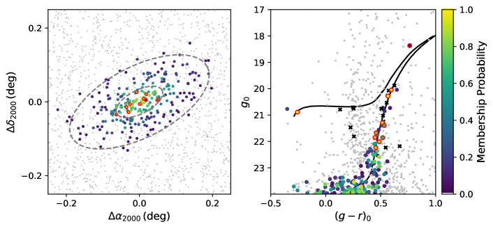
Figure 2: Left: Map of likely member stars in the vicinity of the Leo VI system, with stars colored by their ugali membership probability. Stars with a lower ugali membership probability ($p<0.05$) are shown in grey. Right: Color–magnitude diagram of candidate member stars in the system, again colored by their ugali membership probability. In both plots, we highlight with a red outline stars that are spectroscopically confirmed members of Leo VI (see Section 5) The black crosses denotes sources that have confirmed to be non-members of Leo VI either through their inconsistent spectroscopic radial velocity, high Gaia proper motion or Gaia classification as likely quasar-stellar objects. The black curve represents the ugali best-fit PARSEC isochrone ($\tau\sim$13.3 Gyr, $Z$ = 0.0001, $(m-M)_{0}=20.2$).

Table 1: Measured and derived parameters of Leo VI. Details of each parameter can be found in their corresponding sections.

Parameter	Description	Value	Units
Morphological Fits (Section 4)
$\alpha_{J2000}$	Right Ascension of Centroid	$171.077_{-0.013}^{+0.016}$	deg
$\delta_{J2000}$	Declination of Centroid	$24.874_{-0.011}^{+0.008}$	deg
$a_{h}$	Angular Semi-Major Axis Length	$4.17_{-1.33}^{+1.14}$	arcmin
$a_{1/2}$	Physical Semi-Major Axis Length	$140_{-40}^{+40}$	pc
$r_{h}$	Azimuthally-Averaged Angular Half-Light Radius	$2.84_{-0.9}^{+0.78}$	arcmin
$r_{1/2}$	Azimuthally-Averaged Physical Half-Light Radius	$90_{-30}^{+30}$	pc
$\epsilon$	Ellipticity	$0.54_{-0.29}^{+0.19}$	-
P.A.	Position Angle of Major Axis (East of North)	$63_{-20}^{+13}$	deg
$(m-M)_{0}$	Distance Modulus	$20.23_{-0.07}^{+0.13}$	mag
$D_{\odot}$	Heliocentric Distance	$111_{-4}^{+7}$	kpc
$\tau$	Agea	$>$ 12.37	Gyrs
$M_{V}$	Absolute (Integrated) $V$-band Magnitude	$-3.56_{-0.37}^{+0.47}$	mag
$L_{V}$	$V$-band Luminosity	$2300_{-800}^{+1000}$	$L_{\odot}$
$M_{*}$	Stellar Mass	$2300_{-700}^{+700}$	$M_{\odot}$
Stellar Kinematics and Metallicities (Section 5)
$N_{\rm spec}$	Number of Spectroscopically Confirmed Members	11	-
$v_{\rm hel}$	Heliocentric Radial Velocity	$170.75_{-1.65}^{+1.90}$	km s-1
$\sigma_{v}$	Line-of-Sight Velocity Dispersion	$3.60_{-1.39}^{+1.99}$	km s-1
$M_{1/2}$	Dynamical Mass within half-light radiusb	$1.0_{-0.7}^{+1.6}\times 10^{6}$	$M_{\odot}$
$M_{1/2}/L_{V,1/2}$	Mass to Light Ratio within half-light radiusb	$1000_{-700}^{+1900}$	$M_{\odot}/L_{\odot}$
$[\rm Fe/H]_{\rm spec}$	Mean Spectroscopic Metallicity	$-2.41_{-0.24}^{+0.16}$	dex
$\sigma_{[\rm Fe/H]}$	Metallicity Dispersion	$0.33_{-0.14}^{+0.19}$	dex
Proper Motion, Orbits & J-Factor (Section 6)
$\mu_{\alpha*}$	Proper Motion Right Ascension	$-0.05_{-0.20}^{+0.19}$	mas yr-1
$\mu_{\delta}$	Proper Motion Declination	$-0.22_{-0.17}^{+0.22}$	mas yr-1
$d_{GC}$	Galactocentric Distance	$114_{-6}^{+5}$	kpc
$r_{\rm apo}$	Orbital Apocenter	$210_{-44}^{+190}$	kpc
$r_{\rm peri}$	Orbital Pericenter	$71_{-43}^{+27}$	kpc
$e$	Orbital Eccentricity	$0.65_{-0.07}^{+0.12}$	-
$\log_{10}J(0.5^{\circ})$	J-factor within a solid angle of 0.5∘	$17.1_{-1.2}^{+0.9}$	GeV2cm-5

4 Morphological Fits

To obtain an estimate of the morphological properties of Leo VI and its stellar population, we use the maximum-likelihood-based Ultra–faint GAlaxy LIkelihood toolkit (ugali, Bechtol et al. 2015; Drlica-Wagner et al. 2020) on the followup DECam observations of the system. We model the stellar density profile of the candidate with an elliptical Plummer profile (Plummer, 1911), with the free parameters described by the centroid coordinates ($\alpha_{J2000},\delta_{J2000}$), angular semi-major axis length, $a_{h}$, ellipticity, $\epsilon$, and the position angle (P.A.) of the major axis (defined East of North). We then model the magnitudes and colors of the candidate member stars with PARSEC isochrone model (Bressan et al., 2012; Chen et al., 2014; Tang et al., 2014; Chen et al., 2015) with free parameters being the distance modulus, $(m-M)_{0}$, age, $\tau$, and the metallicity, $Z$, of the candidate system. We also fit another free parameter: stellar richness, $\lambda$, which normalizes the total number of stars in the system (Bechtol et al., 2015; Drlica-Wagner et al., 2020). We use the Markov Chain Monte Carlo sampler emcee (Foreman-Mackey et al., 2013) to simultaneously fit all the stellar density profiles and isochrone parameters in addition to the stellar richness. For star-galaxy separation, we loosen the stellar classification in our ugali analysis by defining stars to be sources with an object class of $0\leq\texttt{EXT\_FITVD}\leq 3$ to include as many Leo VI member candidates as possible in our analysis.

Table 1 shows the values and uncertainties of the stellar density profile and isochrone parameters obtained from ugali. The estimates of parameters are obtained from the median of the marginalized posteriors, while the 1$\sigma$ uncertainties are obtained using the 16th and 84th percentiles. We find that posterior distribution for both the age of the system and the metallicity of the system peaked near the $\tau=13.5$ Gyrs and $Z$ = 0.0001, [Fe/H] $\sim-2.2$ which represents oldest and most metal-poor isochrone in the Bressan et al. (2012) library. We discuss spectroscopic measurements of the metallicity in Section 5.3.

Table 1 also shows Leo VI properties derived from the fitted parameters. For example, we can obtain the azimuthally-averaged angular half-light radius (defined as $r_{h}$ = $a_{h}\sqrt{1-\epsilon}$), the equivalent physical semi-major axis length (in parsec), $a_{1/2}$, and azimuthally-averaged physical half-light radius (in parsec), $r_{1/2}$. Using the prescription defined Martin et al. (2008), we obtain the absolute $V$-band magnitude, $M_{V}$, from the isochrone and use it to derive the $V$-band luminosities ($L_{V}$). We also derive the stellar mass ($M_{*}$) of the system by integrating the best-fit isochrone model assuming an initial mass function from Chabrier (2001).

To investigate the robustness of the fits, we rerun ugali with with different magnitude limit masks ranging from $g<22.5$ to $g<24.5$ mag at intervals 0.5 mag. We find that the fit results for all fitted parameters are consistent within 1$\sigma$ with the uncertainty being generally smaller when using the deeper mask.

For each star, the ugali pipeline assigns a probability that the star is a member of the dwarf galaxy based on its spatial position, photometric properties, and local imaging depth assuming a given model that includes a putative dwarf galaxy and the local stellar field population (Bechtol et al., 2015; Drlica-Wagner et al., 2020). We plot the spatial distribution of stars in a small region around Leo VI, with stars colored by their ugali membership probability in the left plot of Figure 2. While in the right plot of same figure, we show a color-magnitude diagram of the system with its stars colored by their ugali membership probability and also show the best-fit PARSEC isochrone model (Bressan et al., 2012; Chen et al., 2014; Tang et al., 2014; Chen et al., 2015).

Being excellent standard candles (Catelan & Smith, 2015), the presence of RR Lyrae (RRL) stars in Leo VI could be used to obtain an independent and more accurate distance estimate of the system (Martínez-Vázquez et al., 2019). We search the Gaia DR3 (Clementini et al., 2023) and PS1 RRL (Sesar et al., 2018) catalog for RRL stars around Leo VI, but find no RRL stars within 0.2 degrees of the centroid of Leo VI. This is expected as the location of the Horizontal Branch at $g\sim$ 21 is around the magnitude limit of Gaia and thus deeper multi-epoch observations are needed to detect potential RRL stars.

Table 2: Properties of spectroscopically confirmed member stars of Leo VI ordered by decreasing Keck/DEIMOS spectrum S/N. Details of each parameter can be found in Section 5.

Star Name	RA	DEC	$g_{0}$	$r_{0}$	S/N	$v_{\rm hel.}$	$\Sigma$ EW CaT	[Fe/H]	Type
Gaia DR3 3993822846542975360	171.096	24.878	18.36	17.58	66.6	168.9 $\pm$ 1.3	3.53 $\pm$ 0.21	-2.61 $\pm$ 0.11	RGB
Gaia DR3 3993822949622182272	171.048	24.868	20.05	19.44	22.0	164.7 $\pm$ 1.7	2.85 $\pm$ 0.28	-2.51 $\pm$ 0.14	RGB
Gaia DR3 3993823052701408128	171.090	24.882	20.27	19.69	18.9	173.1 $\pm$ 1.8	2.32 $\pm$ 0.37	-2.71 $\pm$ 0.20	RGB
Gaia DR3 3993822502945568128	171.044	24.846	21.29	20.76	7.7	170.2 $\pm$ 3.8	3.07 $\pm$ 0.37	-2.13 $\pm$ 0.19	RGB
Leo VI J112432.23+245250.95	171.134	24.881	21.38	20.83	7.7	172.3 $\pm$ 3.4	3.51 $\pm$ 0.44	-1.91 $\pm$ 0.21	RGB
Leo VI J112431.27+245242.21	171.130	24.878	21.66	21.18	5.8	177.2 $\pm$ 5.3	2.50 $\pm$ 0.52	-2.33 $\pm$ 0.28	RGB
Leo VI J112423.32+245340.09	171.097	24.894	21.83	21.36	4.8	177.9 $\pm$ 6.1	3.07 $\pm$ 0.77	-2.00 $\pm$ 0.38	RGB
Leo VI J112418.58+245204.63	171.077	24.868	20.85	21.08	4.3	177.5 $\pm$ 14.3	-	-	BHB
Leo VI J112401.61+245021.90	171.007	24.839	21.86	21.33	3.9	168.1 $\pm$ 7.6	3.37 $\pm$ 0.64	-1.86 $\pm$ 0.31	RGB
Leo VI J112408.96+245134.74	171.037	24.860	22.01	21.50	3.7	172.3 $\pm$ 7.8	2.05 $\pm$ 0.67	-2.50 $\pm$ 0.39	RGB
Leo VI J112416.48+245400.62	171.069	24.900	22.23	21.75	3.4	179.2 $\pm$ 12.0	1.80 $\pm$ 0.79	-2.60 $\pm$ 0.50	RGB

5 Stellar Kinematics and Metallicities

5.1 Keck Observations

To confirm that Leo VI is a physically bound stellar system and not a chance arrangement of MW stars, we took follow-up spectroscopic observations of the potential member stars with the DEep Imaging Multi-Object Spectrograph (DEIMOS) mounted on the Keck II telescope (Faber et al., 2003).

We obtained 1.0 hour of DEIMOS observations of Leo VI through on the night of 2024 February 14. These observations used a single multi-object mask with slits of width 0.7” and minimum length 4.5”. Targets were selected primarily based on the photometric probabilities provided by a ugali fit to the follow-up DECam imaging, as well as the astrometric information provided by Gaia. We used the DEIMOS 1200G grating and OG550 order blocking filter; this configuration provides $R\approx 6000$ across a wavelength range spanning H$\alpha$, the telluric A-band, and the Calcium Triplet region ($\sim 6500-9000\rm\AA$). All exposures were reduced using the official Keck Data Reduction Pipeline found in the PypeIt software package (Prochaska et al., 2020), with PypeIt’s default flexure correction disabled. Wavelength calibration was performed using XeNeArKr arcs, and flat-fielding used internal quartz flats.

5.2 Line-of-Sight Velocities and Stellar Membership

We obtain the line-of-sight velocities of the potential member stars using the DMOST package (Geha et al., in prep), which is a dedicated measurement pipeline for spectra obtained from DEIMOS 1200G grating. The DMOST package measures line-of-sight velocities by forward modeling the spectrum of a star using both a PHOENIX stellar atmosphere library template (Husser et al., 2013) and a TelFit telluric absorption spectrum template (Gullikson et al., 2014); the latter is used to correct for wavelength shifts induced by the miscentering of stars within their slits. Further details about the velocity measurement procedure implemented within DMOST can be found in (Geha et al., in prep).

Starting from our initial target sample of 42 stars, we were able use the pipeline to obtain line-of-sight velocity measurements for 24 stars. We can see from the left subplot of Figure 3 an excess of 11 stars with a line-of-sight velocity, $v_{\rm hel}$, in the range of 160 kms^-1 $\leq v_{\rm hel}\leq$ 180 kms^-1, which we infer to be the member stars of Leo VI, thus confirming the nature of Leo VI as a gravitationally-bound system. Table 2 shows the basic properties of member stars. Based on their DECam photometry and the best fit ugali isochrone for Leo VI (see Figure 2), we identify these 11 Leo VI member stars as 10 Red Giant Branch (RGB) stars and 1 Blue Horizontal Branch (BHB) star.

We obtain the systemic velocity, $v_{\rm hel}$, and velocity dispersion of the system, $\sigma_{v}$, from the line-of-sight velocity measurements of the 11 member stars using a single two-parameter fit as described in Walker et al. (2006). For the model fit, we apply a uniform prior on the systemic velocity within a range of 164.7 $<v_{\rm hel}<$ 179.2 km s^-1, based on the maximum and minimum range of velocities found in the member stars, and a uniform prior on the velocity dispersion within a range of $\sigma_{v}>0$ km s^-1. Using emcee to obtain the marginalized posterior distribution (shown in Figure 4), we find that the systemic velocity of Leo VI is given by $v_{\rm hel}=170.75_{-1.65}^{+1.90}$ km s^-1, while the velocity dispersion is given by $\sigma_{v}=3.60_{-1.39}^{+1.99}$ km s^-1. The middle subplot of Figure 3 shows the best-fit velocity dispersion model overlaid on the histogram of the measured radial velocity of the Leo VI stars. We find that the velocity dispersion of the system is non-zero (and thus resolved) at a Bayes factor of 7.0 (substantial evidence), and that the 95% Bayesian lower limit of the velocity dispersion is at 1.43 km s^-1. However, there is a small tail in the posterior distribution that is consistent with zero velocity dispersion (see Figure 4).

To test the robustness of the systemic velocity and velocity dispersion measurements from outlier measurements, we performed a jackknife test where we recalculated the parameters for a subsample of stars where one star is removed from the total population at a time. As seen in Figure 5, we found that the values of parameters obtained from the jackknife test are all within the $1\sigma$ of the parameters obtained from the full sample. However, we note that removing the star Gaia DR3 3993822949622182272, does noticeably increase the systemic velocity and decrease the velocity dispersion. If we remove the star from our analysis, the Bayes factor for the non-zero measurement of the velocity dispersion of Leo VI drops to 0.8, and thus disfavoring the resolved velocity dispersion model. As the star Gaia DR3 3993822949622182272 has a relatively low radial velocity of $164.7\pm 1.7$ compared to the rest of the Leo VI member stars, it might be a possible binary or non-member interloper star. Since we only have single-epoch radial velocity measurements, we cannot identify Gaia DR3 3993822949622182272 or the other Leo VI member stars as unresolved binary systems that can inflate the system’s velocity dispersion.

Additionally, if we consider: 1) only using stars with S/N $>$ 5, or 2) using log-uniform priors on the velocity dispersion within a range of $-1<\log_{10}(\sigma_{v})<1$, we find that the systemic velocity and velocity dispersion that are within 1$\sigma$ difference of the original fit.

If we assume that Leo VI is a dispersion-supported system in dynamical equilibrium, we can use the estimator from Wolf et al. (2010) with the non-zero velocity dispersion measurment of Leo VI to calculate its enclosed mass,

$$M_{1/2}=930M_{\odot}\left(\frac{\sigma_{\rm v,los}}{\rm{km\ s}^{-1}}\right)^{2}\left(\frac{r_{1/2}}{\rm{pc}}\right).$$ (1)

We estimate that the dynamical mass of the system within the half-light radius is $1.0_{-0.7}^{+1.6}\times 10^{6}$ $M_{\odot}$. Assuming that the luminosity at half-light radius is given by $L_{1/2}=0.5L_{V}$, we obtain that the mass-to-light-ratio at the half-light radius of Leo VI is given by $1000_{-700}^{+1900}$ $M_{\odot}/L_{\odot}$.

However, the high ellipticity of Leo VI may indicate that the system might be tidally disturbed by the MW, which would make the assumption of dynamical equilibrium invalid. We will further discuss the possibility of Leo VI being a tidally disrupted system in Section 6.2.

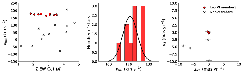
Figure 3: Left: The Equivalent Widths (EWs) of the CaT lines vs. the measured line-of-sight (radial) velocity of the target stars. The plot shows a prominent excess of stars around 160 kms^-1 $\leq v_{\rm hel}\leq$ 180 kms^-1, which we assumed to be members stars of Leo VI. The grey bars show the uncertainties of the line-of-sight (radial) velocity measurement. Middle: Histogram of the measured heliocentric radial velocity of the Leo VI stars overlaid with the best-fit velocity dispersion model (See Section 5.2). The non-Gaussian distribution of the radial velocity of the Leo VI stars is likely caused by small number statistics and the large uncertainties in the velocity measurements. Right: Proper motions of candidate member stars that are bright enough ($g\lesssim 21$) to be measured in Gaia DR3. Three of the spectroscopically confirmed member stars that also contain Gaia proper motion measurements (highlighted in red) are found to be clustered near $\mu_{\delta},\mu_{\alpha}\cos(\delta)\sim(0,0)$  mas/yr.

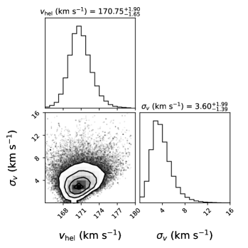
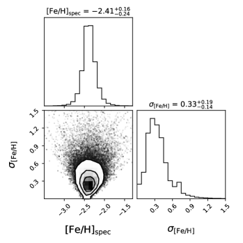
Figure 4: Left: The posterior probability distributions for the systemic heliocentric radial velocity, $v_{hel}$, and velocity dispersion, $\sigma_{v}$, of Leo VI derived using MCMC sampling. Right: The posterior probability distributions for the spectroscopic metallicity, $\mbox{[Fe/H]}_{\rm spec}$, and metallicity dispersion, $\sigma_{\rm[Fe/H]}$, of the system. The posterior distributions favors Leo VI identity as a metal-poor system with non-zero metallicity dispersion and a resolved velocity dispersion measurement.

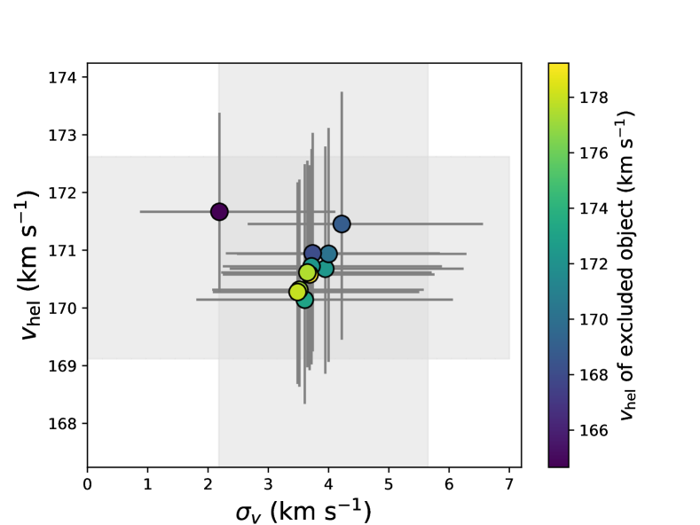
Figure 5: Jackknife test for the radial velocity parameters of Leo VI. The grey regions represent 68% percentile uncertainty of the parameters obtained from the full sample. Each point represents the parameters obtained using a subsample that has excluded one star. All parameters obtained using this test are within 1$\sigma$ of the full sample. The outlier star Gaia DR3 3993822949622182272 ($v_{\rm hel}=164.7\pm 1.7$ km s^-1) might be a possible binary or a non-member interloper.

5.3 Metallicity and Metallicity Dispersion

In addition to the line-of-sight velocities, DMOST also measures the equivalent widths (EWs) of the infrared Ca II triplet (CaT) lines. In this analysis, we model the CaT lines of high S/N stars (${\rm S/N}>15$) with a combination of Gaussian and Lorentzian models, while we model the rest of the stars with a single Gaussian model. We note that our EW measurements are only valid for RGB stars, so we exclude the EW CaT measurement for the BHB star.

We derived [Fe/H] metallicities from the EWs using the calibration relation from Carrera et al. (2013). The calibration relation requires the absolute $V$-band magnitude for each star, which we obtain using their $g$ and $r$ band magnitudes from the follow-up DECam catalog. We then convert the $g$ and $r$ magnitudes into relative $V$-band magnitude using transformation relations from Abbott et al. (2021) and subtract the relative magnitudes with distance modulus from the ugali fit (Table 1) to obtain the absolute $V$-band magnitudes.

We derive the systemic metallicity and metallicity dispersion of Leo VI using emcee with a similar two-parameter fit as described for the systemic velocity. We apply a uniform prior on both the spectroscopic metallicity of the system and the metallicity dispersion within the range of $-4<[\rm Fe/H]_{\rm spec}<$ 0 and $0<\sigma_{[\rm Fe/H]}<$ 3, respectively. Using metallicity measurements for 6 high S/N member stars (S/N $>5$), we find that the systemic spectroscopic metallicity of Leo VI is ${[\rm Fe/H]_{\rm spec}=-2.41_{-0.24}^{+0.16}}$ and a metallicity dispersion at $\sigma_{[\rm Fe/H]}={0.33_{-0.14}^{+0.19}}$ (see Figure 4). We find a non-zero metallicity dispersion for the system with a Bayes factor of 5.5 (substantial evidence) and place a 95% Bayesian lower limit of the metallicity dispersion at 0.10.

As with the velocity dispersion measurement, we repeated the analysis with log-uniform priors on the metallicity dispersion within a range of $-2<\log_{10}{(\sigma_{[\rm Fe/H]})}<0.5$ and find that the metallicity and metallicity dispersion is within 1$\sigma$ difference of the original values, with the dispersion values dropping to $\sigma_{[\rm Fe/H]}={0.22_{-0.12}^{+0.18}}$. As with the velocity dispersion, we see that there is a small tail in the posterior distribution that is consistent with zero metallicity dispersion.

As shown in Figure 6, we find the size-luminosity, luminosity-metallicity, and luminosity-velocity dispersion relation of Leo VI to be consistent with other MW satellite galaxies.

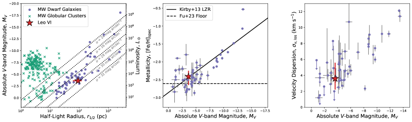
Figure 6: Left: The absolute $V$-band magnitude, $M_{V}$, vs. the azimuthally-averaged physical half-light radius, $r_{1/2}$, of Leo VI and the population of known Local Group globular clusters and dwarf galaxies. Leo VI’s morphological properties are consistent with those of a dwarf galaxy. Middle: The systemic metallicity, [Fe/H], vs.  the absolute $V$-band magnitude of Leo VI and the population of Local Group dwarf galaxies. The overlaid black line represents the $V$-band absolute Luminosity-Metallicity Relation (LZR) found in Kirby et al. (2013), while the dashed black line represents the metallicity floor of [Fe/H] $=-2.61$ proposed for faint systems (Fu et al., 2023) Right: The line-of-sight velocity dispersion, $\sigma_{\rm v,los}$, vs. absolute $V$-band magnitude of the population of Local Group dwarf galaxies.

6 Discussion

There are several unique properties of Leo VI that make its discovery particularly interesting, namely its highly elliptical shape and proximity to other MW satellites. We first discuss the orbital properties of Leo VI derived by combining Keck radial velocity measurements with Gaia proper motion measurements in Section 6.1. We then discuss whether Leo VI’s elliptical shape might indicate that it is undergoing tidal disruption in Section 6.2. In Section 6.3, we consider the possibility of Leo VI being part of a group infall scenario due to its proximity to other satellite galaxies in the constellations of Leo and Crater.

6.1 Proper Motion and Orbit of Leo VI

To obtain three-dimensional velocity information of the system, we cross-match our DECam-based stellar catalog with the Gaia DR3 (Gaia Collaboration et al., 2023). As shown in the right subplot of Figure 3, all 3 spectroscopically confirmed member stars of Leo VI which also have Gaia proper motion measurements have proper motions clustered near $\mu_{\delta},\mu_{\alpha}\cos(\delta)\sim(0,0)$  mas/yr, further confirming that it is a gravitationally-bound system that is located far from the MW. Using emcee to fit a Gaussian mixture model and taking into account for the correlations in $\mu_{\alpha*}$ and $\mu_{\delta}$, we find that the systemic proper motion of Leo VI is $\mu_{\alpha*}=-0.05_{-0.20}^{+0.19}$ mas yr^-1 and $\mu_{\delta}=-0.22_{-0.17}^{+0.22}$ mas yr^-1. However, at a heliocentric distance of ${D=111_{-4}^{+7}}$  kpc proper motion uncertainties of 0.2 mas/yr corresponds to velocities uncertainties of $\sim$100 km s^-1.

To determine the orbit of Leo VI, we integrated 1,000 realizations of its orbit using the gala galactic dynamics package (Price-Whelan, 2017). We obtain a sample of the possible current 6-D positions and velocities ($\alpha_{J2000}$, $\delta_{J2000}$, $D_{\odot}$, $\mu_{\alpha*}$, $\mu_{\delta}$, $v_{\rm hel}$) of the system by sampling from the Gaussian error distribution of the observed position and velocity parameters (see Table 1), and convert it to the astropy v4.0 Galactrocentric Frame (Astropy Collaboration et al., 2013). We then rewind Leo VI’s orbit back in time for 10 Gyrs in the presence of gala’s MilkyWayPotential model (Bovy, 2015) and recorded gala’s estimate of the orbital parameters of Leo VI. We find an orbital apocenter of $210_{-44}^{+190}$ kpc, while the pericenter is $71_{-43}^{+27}$ kpc and the orbital eccentricity is $0.65_{-0.07}^{+0.12}$. Moreover, the z-component of the specific angular momentum, $L_{z}$, and the specific orbital energy of the system, $E$, are given by $L_{z}=-4.09\ \pm$ 4.76 kpc² Myr^-1 and $E=-0.025\ \pm 0.018$ kpc² Myr^-2, respectively. We further find that 86.5% of realizations of Leo VI’s orbit is bounded ($E<0$ kpc² Myr^-2) and 80.7% of realizations yield a prograde orbit.

6.2 Possible Tidal Disruption

Due to the high ellipticity of Leo VI, coupled with the fact that the direction of systemic proper motion aligns with the semi-major axis (see left panel of Figure 8), we discuss the possibility of the system being tidally disturbed by the MW. Common dynamical mass estimators for UFDs (such as Wolf et al. 2010) are based on the assumption that the system is in dynamical equilibrium, which doesn’t apply to disrupting systems. Therefore, determining whether the system is in dynamical equilibrium or has been tidally disturbed has important implications for measurements of its dark matter content.

To assess whether the system is experiencing tidal disruption, we follow the methodology of Pace et al. (2022) and compare the average density of Leo VI within its half-light radius, ${\rho_{1/2}=1.6_{-1.2}^{+5.4}\times 10^{8}M_{\odot}}$ kpc^-3, to twice the average MW density at its orbital pericenter $2\rho_{MW}(r=r_{\rm peri})=7.4\times 10^{5}M_{\odot}$ kpc^-3. If we assume a flat rotation curve for the MW and that Leo VI has an circular orbit, this comparison is equivalent to comparing the half-light radius of the system with its Jacobi (or tidal) radius where beyond it the tidal forces exceed the systems own gravitational force. As illustrated in Figure 7, the average density Leo VI is much higher than twice the average MW density. Therefore, Leo VI’s Jacobi radius is likely larger than its half-light radius even when it is at its orbital pericenter, and that it is unlikely that the system is tidally disrupting. This conclusion also holds even when using 1$\sigma$ lower bound for both the average density of Leo VI and pericenter distance. However, we note that this approximation does not hold for all systems as the FIRE simulation has found the presences of high density satellites galaxies which are still tidally disrupting (Shipp et al., 2023). In addition, Figure 7 shows the measured 3D velocity of Leo VI with other nearby satellites compared to the local escape velocity of gala’s MilkyWayPotential potential. It is likely that Leo VI is a bound system and that it is not on first infall, allowing the possibility of the system to reach its pericenter (at $71_{-43}^{+27}$ kpc) in the past.

Another signature of a tidally disrupting system is the presence of a velocity gradient in its member stars. Figure 8 illustrates the radial velocity of the spectroscopically confirmed member stars of Leo VI as a function of its on-sky position and distance along the semi-major axis. To measure the velocity gradient of the system, we use a linear model to fit the radial velocity of the Leo VI’s members stars as a function of its distance along the semi-major axis while taking account of intrinsic scatter.

Using emcee to sample the posterior of the linear model, we find a very large velocity gradient of $73^{+46}_{-48}$ km s^-1/deg, albeit with large uncertainties. However, the apparent non-zero velocity gradient measurement only has a marginal Bayes factor of 3.1. Moreover, if we remove the possible binary or non-member star Gaia DR3 3993822949622182272 from our sample, the velocity gradient drops to $34^{+52}_{-54}$ km s^-1/deg, with the non-zero velocity gradient model being disfavored at a Bayes factor of of 0.8. Due to the small angular extent of Leo VI on the sky ($r_{h}=2.84_{-0.9}^{+0.78}$ arcmin), we are unable to conclusively determine the existance or absence of a velocity gradient, and thus more measurements of the Leo VI’s members stars is needed to conclusively determine if Leo VI is tidally disrupting or not.

Moreover, both observations of MW satellites (Pace et al., 2022) and N-body simulations (Muñoz et al., 2008) has found no strong correlation between the ellipticity of the system and whether it is tidal disrupting. Pace et al. (2022) also observed that the proper motion vector of highly elliptical UFDs often aligns with its semi-major axis even for non-disrupting systems with large pericenters.

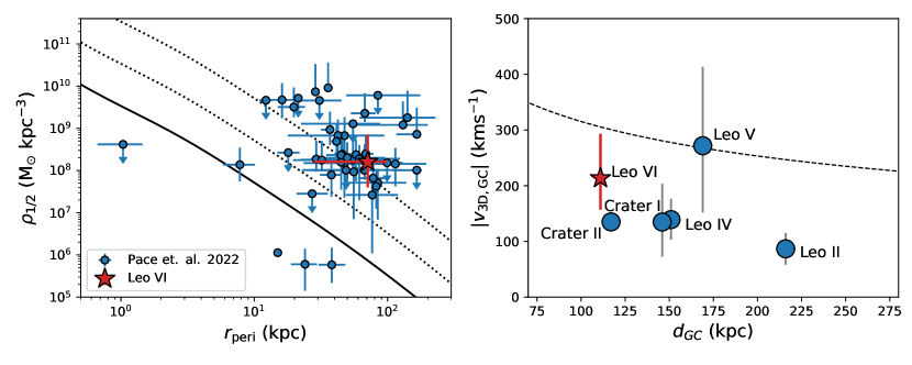
Figure 7: Left: The average density within a half-light radius, $\rho_{1/2}$, vs. distance of pericenter, $r_{\rm peri}$, of Leo VI and other MW satellites (Pace et al., 2022). The solid black line represent twice the enclosed MW density as a function of radius, while the dashed lines represent 20 and 200 times the enclosed MW density. If a satellite is located below the solid line, its half-light radius is estimated to be bigger than its Jacobi (tidal) radius and it is likely to be tidally disrupting (Pace et al., 2022). Right: The magnitude of the 3D Galactocentric velocity, $|V_{\rm 3D,GC}|$, vs. the Galactocentric distance, $d_{\rm GC}$, of Leo VI and other nearby satellite galaxies. The dashed lines represented the escape velocity of the potentials from the gala’s MilkyWayPotential potential. Leo VI is likely a bound system, and thus it is likely to have reached its orbital pericenter at least once in the past.

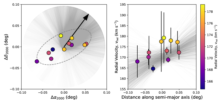
Figure 8: Left: Spatial distribution of the spectroscopically confirmed Leo VI member stars with points colored by the measured line-of-sight (radial) velocity. The dashed ellipse shows the half-light radius of Leo VI. The direction of the median systemic proper motion (after correcting for solar reflex motion), computed from the three spectroscopically confirmed members with Gaia proper motion measurements, are shown with the black arrow, while the faint gray lines represent the 1,000 Monte Carlo samplings from the proper motion uncertainties. The direction of proper motion aligns with the semi-major axis of Leo VI. Right: The line-of-sight (radial) velocity of Leo VI member stars as a function of distance along its semi-major axis. The gray lines represent the Monte Carlo samplings used to measure the radial velocity gradient of the system along the semi-major axis. Due to the low number statistics and high uncertainty of the radial velocity measurements, we are unable to conclusively determine the presence/absence of a velocity gradient.

6.3 Group Infall scenario

The on-sky location of Leo VI is close to several other known distant MW satellite galaxies that are already found in the constellations Leo and Leo Minor. Due to their similar on-sky positions and radial velocity, it has been suggested that the MW satellite galaxies in Leo (Leo II, Leo IV, Leo V), the star cluster Crater/Laevens 1, and the dwarf galaxy Crater II might have been accreted into the MW through a group infall scenario (Torrealba et al., 2016; Pawlowski, 2021; Júlio et al., 2024). Moreover, simulations from Li & Helmi (2008) have shown that about one-third of subhaloes are accreated into the MW through infall groups. In this section, we discuss the possibility of Leo VI and other close-by systems such Leo Minor I (Cerny et al., 2023a), Hydra II (Martin et al., 2015) and Centaurus I (Mau et al., 2020) being members of the proposed Leo-Crater infall group.

Torrealba et al. (2016) found that the member systems of the Leo-Crater infall group are all located close to the great circle with the pole at ($\alpha,\delta$) = (83.2^∘, $-$11.8^∘) and forms a consistent heliocentric distance gradient as a function of their declination. Figure 9 shows the heliocentric distance of Leo VI and the other members of the infall group as a function of their spatial distribution. From the figure, we can see that both Leo VI and especially Leo Minor I are too close to follow the heliocentric distance gradient exhibited by the other members of the infall group. While the distances of Hydra II and Centaurus I are more consistent with the other members of the group, their distances are not consistent with the distance trend from Torrealba et al. (2016).

We expect that satellites that are accreted into the MW via an infall group to share similar values of total energy and angular momentum (Lynden-Bell & Lynden-Bell, 1995). Using gala’s MilkyWayPotential model and the velocity measurements of the Leo-Crater group collected from Júlio et al. (2024), we calculated the specific angular momentum and specific energy distribution of the member satellites of the Leo-Crater group. For Hydra II and Centaurus I, we use proper motion and radial velocity measurements from Kirby et al. (2015); Pace et al. (2022) and Heiger et al. (2024), respectively. We exclude Leo Minor I from the following analysis due to the lack of radial velocity measurements. As shown in Figure 10, the distribution of specific energy, $E$, and the square of the specific angular momentum squared, $L^{2}$, of 4 satellites (Leo II, Leo IV, Leo V and Crater) all intersect each other at $(L^{2},E)\sim$ (780 kpc⁴ Myr^-2 , -0.023 kpc² Myr^-2) suggesting a common origin (Pawlowski, 2021). We find that the $E-L^{2}$ distribution of Crater II, Leo VI, Hydra II and Centaurus I is inconsistent with the other satellites of the group. However, as shown in Figure 10, the specific energy, $E$, and z-component of specific angular momentum $E-L_{z}$ distribution of Leo VI is consistent with all the other members of the proposed group (including Crater II). Although this is mostly due to the large uncertainties in the proper motion measurement of Leo VI as Crater II has a inconsistent $E-L_{z}$ distribution with some of the other members of the infall group such as Leo II and Leo IV.

Systems that are part of an infall group are also expected to have similar orbital poles or direction of angular momentum. Júlio et al. (2024) found that 4 systems in the proposed Leo-Crater Group (Leo II, Leo IV, Leo V and Crater) have orbital poles that all intersect with each other, while position of the orbital poles of Crater II doesn’t not match the other members of the system. As shown in Figure 11, the position of the orbital pole of Leo VI is consistent with the group orbital pole of the Leo-Crater infall group at $(\alpha_{J2000},\delta_{J2000})\sim(210^{\circ},-24^{\circ})$ while Hydra II also has orbital pole that is somewhat close by ($\sim 6\deg$ away). As with the energy-angular momentum distributions, we find that position orbital pole of Centuarus I is inconsistent with the other members of the proposed group.

While Leo VI shares a similar on-sky position, orbital pole location and $E-L_{z}$ distribution with the members of the Leo-Crater infall group, due to its relatively close distance and inconsistent $E-L^{2}$ distribution with the other members of the group, we determine that it is unlikely for Leo VI being a part of the the proposed infall group. However, more precise measurements of the proper motion of Leo VI are needed to more definitely determine the its membership in the Leo-Crater group. Similarly, we also did not find convincing evidence that Leo Minor I, Hydrus II and Centuarus I are part Leo-Crater infall group due to their inconsistent heliocentric distance, $E-L^{2}$ distribution and orbital pole location with the infall group.

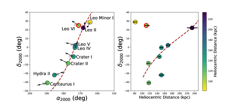
Figure 9: Left: Spatial distribution of Leo VI and other potential members of the Crater-Leo infall group. The markers are colored based on the heliocentric distance of the system. The black arrows represent the direction of the median systemic proper motion of the system (after correcting for solar reflex motion), while the faint grey lines represent the 1,000 Monte Carlo samplings from the proper motion uncertainties. The proper motion for the members of the Crater-Leo infall group were obtained from Júlio et al. (2024), where we have use their Hubble Space Telescope measurements for Leo IV and Leo V. The brown line represents a great circle with a pole centered at (83.2^∘, -11.8^∘) that passes close to the members of the infall group (Torrealba et al., 2016). Right: The Heliocentric distance of Leo VI and the nearby satellites as a function of the declination, $\delta_{2000}$. The brown line shows the orbit of the proposed Leo-Crater group from Torrealba et al. (2016). The plots indicate that the heliocentric distances of Leo VI and Leo Minor I are inconsistent with the distance gradient followed by the members of the Crater-Leo group.

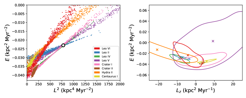
Figure 10: Left: The specific energy, $E$, vs. the square of the specific angular momentum, $L^{2}$, of Leo VI and the members of the Crater-Leo infall group. We find that the $E-L^{2}$ distribution of Leo II, Leo IV, Leo V, and Crater all intersect at $(L^{2},E)\sim$ (780 kpc⁴ Myr^-2 , $-0.023$ kpc² Myr^-2), suggesting a common origin (Pawlowski, 2021). The $E-L^{2}$ distribution of Leo VI is inconsistent with the other infall group members, suggesting that it may not be part of the group. Right: The specific energy, $E$, vs. the z-component of the specific angular momentum, $L_{z}$, of Leo VI and the other satellites. The cross markers represent the median $E-L_{z}$ values of the satellites, while the contour lines represent the 1$\sigma$ uncertainty. $E-L_{z}$ distribution of Leo VI is consistent with all the other members of the Crater-Leo infall group, albeit with large uncertainties.

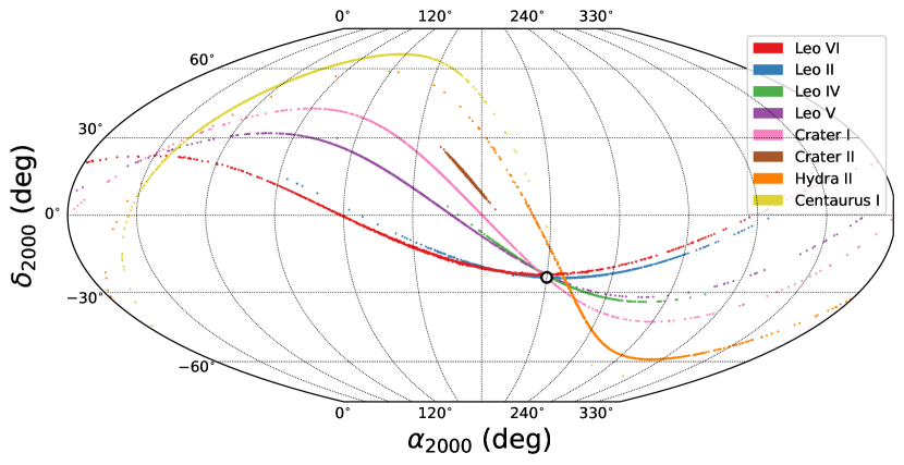
Figure 11: Distribution of the possible orbital poles of Leo VI and the other possible members of the Crater-Leo infall group. The position of the orbital pole of Leo VI is consistent with the possible group orbital pole of the Crater-Leo group (Leo II, Leo IV, Leo V and Crater) at $(\alpha_{J2000},\delta_{J2000})\sim(210^{\circ},-24^{\circ})$, while the position of the orbital pole of Crater II is inconsistent with the group orbital pole.

6.4 Astrophysical J-factor

As mentioned in Section 1, MW satellite UFDs are also useful targets for searches for dark matter annihilation or decay products (Ackermann et al., 2015; Geringer-Sameth et al., 2015b; McDaniel et al., 2023; Boddy et al., 2024). The astrophysical component that governs the dark matter annihilation and decay fluxes are referred to as the J-factor and D-factor, respectively. Both factors depend on the dark matter density of the system along the line of sight such that $J(\theta)=\iint_{\rm los}\rho_{\rm DM}^{2}\rm{d}l\rm{d}\Omega$ and $D(\theta)=\iint_{\rm los}\rho_{\rm DM}\rm{d}l\rm{d}\Omega$, where $\rho_{\rm DM}$ is the dark matter density, $\rm{d}l$ is the line-of-sight direction and $\rm{d}\Omega$ is the solid angle with radius $\theta$.

We use the framework developed by Bonnivard et al. (2015); Geringer-Sameth et al. (2015a); Pace & Strigari (2019) to calculate the J-factor and D-factor of Leo VI. We model the system with a stellar component parameterized by a Plummer distribution (Plummer, 1911) and dark matter component with a Navarro–Frenk–White profile (Navarro et al., 1997) while assuming a constant stellar anisotropy with radius. We then fit the dark matter profile by modelling the velocity dispersion of the member stars using the spherical Jeans equations and compared them with the measured velocity dispersion from the spectroscopic observations.

For the J-factor of Leo VI, we find $\log_{10}{J(\theta)}=16.9_{-1.1}^{+0.9}$, $17.0_{-1.1}^{+0.9}$, $17.1_{-1.2}^{+0.9}$, and $17.1_{-1.2}^{+0.9}$ for solid angles of $\theta=0.1^{\circ},0.2^{\circ},0.5^{\circ},1^{\circ}$ in logarithmic units of ${\rm GeV^{2}~{}cm^{-5}}$. These J-factor measurements are consistent with estimates of $\log_{10}(J(0.5^{\circ}))=17.3_{-1.2}^{+0.7}$, obtained from the empirical scaling relation derived in Pace & Strigari (2019),

$$\frac{J(0.5^{\circ})}{\rm GeV^{2}~{}cm^{-5}}=10^{17.87}\left(\frac{\sigma_{\rm v,los}}{\rm{5~{}kms}^{-1}}\right)^{4}\left(\frac{D_{\odot}}{\rm{100~{}kpc}}\right)^{-2}\left(\frac{r_{1/2}}{\rm{100~{}pc}}\right)^{-1}.$$ (2)

For the D-factor of Leo VI, we find $\log_{10}{D(\theta)}=16.5_{-0.6}^{+0.5}$, $16.9\pm 0.6$, and $17.3\pm 0.7$, for solid angles of $\theta=0.1^{\circ},0.2^{\circ},0.5^{\circ}$ in logarithmic units of ${\rm GeV~{}cm^{-2}}$. As the velocity dispersion has a tail to zero velocity dispersion (see Figure 4), the J-factor and D-factor also have similar tails. We have applied a $V_{\rm max}>1~{}{\rm km~{}s^{-1}}$ cut to remove the tail and note that without this change the J-factor and D-factor decrease by roughly 0.05 dex.

While Leo VI does not have a large J-factor compared to other MW UFDs, for example Wilman 1 and Ursa Major II have J-factors of $\log_{10}J(0.5^{\circ})=19.53_{-0.50}^{+0.50}$ and $19.44_{-0.39}^{+0.41}$ GeV²cm^-5, respectively (Pace & Strigari, 2019), it could be included in a stacked analysis with other UFDs.

7 Summary

We have presented the DELVE EDR3 data set and used it to discover the MW satellite Leo VI. Using the ugali maximum likelihood-fit of the systems morphology and color-magnitude diagram, we find that Leo VI is an old ($\tau>$12.37 Gyrs), metal-poor ($\mbox{[Fe/H]}_{\rm spec}=-2.41_{-0.24}^{+0.16}$), stellar system with low luminosity ($M_{V}=-3.56_{-0.37}^{+0.47}$ mag), large size ($r_{1/2}=90_{-30}^{+30}$ pc), elliptical shape ($\epsilon=0.54_{-0.29}^{+0.19}$) and a large heliocentric distance ($D=111^{+9}_{-4}$  kpc). By obtaining Keck/DEIMOS spectroscopy of the possible member stars of Leo VI, we are able to find 11 member stars for the system (with line-of-sight velocities of 160 kms^-1 $\leq v_{\rm hel}\leq$ 180 kms^-1), and find a non-zero velocity dispersion of $3.60_{-1.39}^{+1.99}$ km s^-1. We are also able to obtain orbital properties of Leo VI by combining proper motion measurements from Gaia DR3 ($\mu_{\alpha*}=-0.05_{-0.20}^{+0.19}$ mas yr^-1, $\mu_{\delta}=-0.22_{-0.17}^{+0.22}$ mas yr^-1) with the system’s measured radial velocity of $v_{\rm hel}=170.75_{-1.65}^{+1.90}$ km s^-1.

Since their discovery in SDSS, there has been considerable uncertainty in the classification of some ultra-faint MW satellites as either UFDs or globular clusters (Simon, 2019). As illustrated in Figure 6, the half-light radius of Leo VI ($r_{1/2}=90_{-30}^{+30}$ pc) is bigger than all known Milky Way globular clusters, likely indicating its identity as an UFD. Compared to globular clusters, UFDs also have much higher amounts of dark matter (Simon, 2019). Thus, Leo VI’s identity as an UFD is further supported by its high mass to light ratio of $1000_{-700}^{+1900}M_{\odot}/L_{\odot}$ and its non-zero metallicity dispersion measurement of $\sigma_{[\rm Fe/H]}=0.33_{-0.14}^{+0.19}$, which suggest the presence of a dark matter halo massive enough to retain the supernove ejecta needed for multiple generations of star formation (Simon, 2019).

Despite the system’s highly elliptical shape and the alignment of its proper motion vector with the semi-major axis, we have found that Leo VI’s average density within its half-light radius is much larger than average MW density at its orbital pericenter, disfavoring the idea that the system is undergoing disruption. Moreover, we could not conclusively determine the presence or absence of a velocity gradient within the system due to the large uncertainties and low number of radial velocity measurements of Leo VI’s member stars. The system also has an on-sky location that is close to other members of the proposed Crater-Leo infall group. However, it is improbable that Leo VI is a part of this group as its heliocentric distance and energy-angular momentum ($E-L^{2}$) distribution do not match the distribution found in other members.

Leo VI is the fourteenth ultra-faint MW satellite found in DELVE data (Mau et al. 2020; Cerny et al. 2021a, b, 2023a, 2023b, 2023c; Cerny et al., in prep). However, unlike the other DELVE satellites, it was found in the preliminary data from the DELVE EDR3 catalog, which features deeper and more accurate photometric measurements than previous DELVE releases (Drlica-Wagner et al., 2022). Therefore, it is expected that a more comprehensive dwarf galaxy search of the upcoming full DELVE Data Release 3 catalogue will yield many more new MW satellite discoveries. Manwadkar & Kravtsov (2022) forecasted that the final DELVE-WIDE survey is expected to find $64_{-13}^{+17}$ MW satellites with $M_{V}<0$ and $r_{1/2}>$ 10 pc at $\delta_{J2000}<0$ deg, while only 35 systems have been discovered in this region so far. Furthermore, it is expected that the upcoming Vera C. Rubin Observatory’s Legacy Survey of Space and Time (Ivezić et al., 2019) will discover hundreds of UFDs in the local volume (Hargis et al., 2014; Mutlu-Pakdil et al., 2021; Manwadkar & Kravtsov, 2022). Space-based telescopes such as Roman (Spergel et al., 2015) and Euclid (Euclid Collaboration et al., 2022) are also expected to have the potential of finding more ultra-faint dwarf galaxies (Nadler et al., 2024). This growing population of known UFDs in the Local Group will allow us to probe the matter power spectrum to even smaller scales and provide insight into the process of galaxy formation for the smallest galaxies.

References

- Abbott et al. (2021) Abbott, T. M. C., Adamów, M., Aguena, M., et al. 2021, ApJS, 255, 20, doi: 10.3847/1538-4365/ac00b3
- Ackermann et al. (2015) Ackermann, M., Albert, A., Anderson, B., et al. 2015, Physical Review Letters, 115, 231301, doi: 10.1103/PhysRevLett.115.231301
- Astropy Collaboration et al. (2013) Astropy Collaboration, Robitaille, T. P., Tollerud, E. J., et al. 2013, A&A, 558, A33, doi: 10.1051/0004-6361/201322068
- Astropy Collaboration et al. (2018) Astropy Collaboration, Price-Whelan, A. M., Sipőcz, B. M., et al. 2018, AJ, 156, 123, doi: 10.3847/1538-3881/aabc4f
- Bechtol et al. (2015) Bechtol, K., Drlica-Wagner, A., Balbinot, E., & Pieres. 2015, ApJ, 807, 50
- Belokurov et al. (2007) Belokurov, V., Zucker, D. B., Evans, N. W., et al. 2007, ApJ, 654, 897, doi: 10.1086/509718
- Belokurov et al. (2008) Belokurov, V., Walker, M. G., Evans, N. W., et al. 2008, ApJ, 686, L83, doi: 10.1086/592962
- Bernstein et al. (2017) Bernstein, G. M., Abbott, T. M. C., Desai, S., et al. 2017, PASP, 129, 114502, doi: 10.1088/1538-3873/aa858e
- Bertin (2006) Bertin, E. 2006, in Astronomical Society of the Pacific Conference Series, Vol. 351, Astronomical Data Analysis Software and Systems XV, ed. C. Gabriel, C. Arviset, D. Ponz, & S. Enrique, 112
- Bertin (2011) Bertin, E. 2011, in Astronomical Society of the Pacific Conference Series, Vol. 442, Astronomical Data Analysis Software and Systems XX, ed. I. N. Evans, A. Accomazzi, D. J. Mink, & A. H. Rots, 435
- Bertin & Arnouts (1996) Bertin, E., & Arnouts, S. 1996, A&AS, 117, 393, doi: 10.1051/aas:1996164
- Bertin et al. (2002) Bertin, E., Mellier, Y., Radovich, M., et al. 2002, in Astronomical Society of the Pacific Conference Series, Vol. 281, Astronomical Data Analysis Software and Systems XI, ed. D. A. Bohlender, D. Durand, & T. H. Handley, 228
- Boddy et al. (2024) Boddy, K. K., Carter, Z. J., Kumar, J., et al. 2024, Phys. Rev. D, 109, 103007, doi: 10.1103/PhysRevD.109.103007
- Bonnivard et al. (2015) Bonnivard, V., Combet, C., Daniel, M., et al. 2015, MNRAS, 453, 849, doi: 10.1093/mnras/stv1601
- Bovy (2015) Bovy, J. 2015, ApJS, 216, 29, doi: 10.1088/0067-0049/216/2/29
- Brandt (2016) Brandt, T. D. 2016, ApJ, 824, L31, doi: 10.3847/2041-8205/824/2/L31
- Bressan et al. (2012) Bressan, A., Marigo, P., Girardi, L., et al. 2012, MNRAS, 427, 127, doi: 10.1111/j.1365-2966.2012.21948.x
- Bullock & Boylan-Kolchin (2017) Bullock, J. S., & Boylan-Kolchin, M. 2017, ARA&A, 55, 343, doi: 10.1146/annurev-astro-091916-055313
- Carrera et al. (2013) Carrera, R., Pancino, E., Gallart, C., & del Pino, A. 2013, MNRAS, 434, 1681, doi: 10.1093/mnras/stt1126
- Catelan & Smith (2015) Catelan, M., & Smith, H. A. 2015, Pulsating Stars
- Cerny et al. (2021a) Cerny, W., Pace, A. B., Drlica-Wagner, A., et al. 2021a, ApJ, 920, L44, doi: 10.3847/2041-8213/ac2d9a
- Cerny et al. (2021b) —. 2021b, ApJ, 910, 18, doi: 10.3847/1538-4357/abe1af
- Cerny et al. (2023a) Cerny, W., Martínez-Vázquez, C. E., Drlica-Wagner, A., et al. 2023a, ApJ, 953, 1, doi: 10.3847/1538-4357/acdd78
- Cerny et al. (2023b) Cerny, W., Simon, J. D., Li, T. S., et al. 2023b, ApJ, 942, 111, doi: 10.3847/1538-4357/aca1c3
- Cerny et al. (2023c) Cerny, W., Drlica-Wagner, A., Li, T. S., et al. 2023c, ApJ, 953, L21, doi: 10.3847/2041-8213/aced84
- Chabrier (2001) Chabrier, G. 2001, ApJ, 554, 1274, doi: 10.1086/321401
- Chambers et al. (2016) Chambers, K. C., Magnier, E. A., Metcalfe, N., et al. 2016, arXiv e-prints, arXiv:1612.05560, doi: 10.48550/arXiv.1612.05560
- Chen et al. (2015) Chen, Y., Bressan, A., Girardi, L., et al. 2015, MNRAS, 452, 1068, doi: 10.1093/mnras/stv1281
- Chen et al. (2014) Chen, Y., Girardi, L., Bressan, A., et al. 2014, MNRAS, 444, 2525, doi: 10.1093/mnras/stu1605
- Clementini et al. (2023) Clementini, G., Ripepi, V., Garofalo, A., et al. 2023, A&A, 674, A18, doi: 10.1051/0004-6361/202243964
- Dark Energy Survey Collaboration et al. (2016) Dark Energy Survey Collaboration, Abbott, T., Abdalla, F. B., et al. 2016, MNRAS, 460, 1270, doi: 10.1093/mnras/stw641
- Dey et al. (2019) Dey, A., Schlegel, D. J., Lang, D., et al. 2019, AJ, 157, 168, doi: 10.3847/1538-3881/ab089d
- Drlica-Wagner et al. (2015) Drlica-Wagner, A., Bechtol, K., Rykoff, E. S., et al. 2015, ApJ, 813, 109, doi: 10.1088/0004-637X/813/2/109
- Drlica-Wagner et al. (2020) Drlica-Wagner, A., Bechtol, K., Mau, S., et al. 2020, ApJ, 893, 47, doi: 10.3847/1538-4357/ab7eb9
- Drlica-Wagner et al. (2021) Drlica-Wagner, A., Carlin, J. L., Nidever, D. L., et al. 2021, ApJS, 256, 2, doi: 10.3847/1538-4365/ac079d
- Drlica-Wagner et al. (2022) Drlica-Wagner, A., Ferguson, P. S., Adamów, M., et al. 2022, ApJS, 261, 38, doi: 10.3847/1538-4365/ac78eb
- Euclid Collaboration et al. (2022) Euclid Collaboration, Scaramella, R., Amiaux, J., et al. 2022, A&A, 662, A112, doi: 10.1051/0004-6361/202141938
- Everett et al. (2022) Everett, S., Yanny, B., Kuropatkin, N., et al. 2022, ApJS, 258, 15, doi: 10.3847/1538-4365/ac26c1
- Faber et al. (2003) Faber, S. M., Phillips, A. C., Kibrick, R. I., et al. 2003, in Society of Photo-Optical Instrumentation Engineers (SPIE) Conference Series, Vol. 4841, Instrument Design and Performance for Optical/Infrared Ground-based Telescopes, ed. M. Iye & A. F. M. Moorwood, 1657–1669, doi: 10.1117/12.460346
- Flaugher et al. (2015) Flaugher, B., Diehl, H. T., Honscheid, K., et al. 2015, submitted to AJ. https://arxiv.org/abs/1504.02900
- Foreman-Mackey (2016) Foreman-Mackey, D. 2016, The Journal of Open Source Software, 1, 24, doi: 10.21105/joss.00024
- Foreman-Mackey et al. (2013) Foreman-Mackey, D., Hogg, D. W., Lang, D., & Goodman, J. 2013, PASP, 125, 306, doi: 10.1086/670067
- Fu et al. (2023) Fu, S. W., Weisz, D. R., Starkenburg, E., et al. 2023, ApJ, 958, 167, doi: 10.3847/1538-4357/ad0030
- Gaia Collaboration et al. (2018) Gaia Collaboration, Brown, A. G. A., Vallenari, A., et al. 2018, A&A, 616, A1, doi: 10.1051/0004-6361/201833051
- Gaia Collaboration et al. (2023) Gaia Collaboration, Vallenari, A., Brown, A. G. A., et al. 2023, A&A, 674, A1, doi: 10.1051/0004-6361/202243940
- Geringer-Sameth et al. (2015a) Geringer-Sameth, A., Koushiappas, S. M., & Walker, M. 2015a, ApJ, 801, 74, doi: 10.1088/0004-637X/801/2/74
- Geringer-Sameth et al. (2015b) Geringer-Sameth, A., Koushiappas, S. M., & Walker, M. G. 2015b, Phys. Rev. D, 91, 083535, doi: 10.1103/PhysRevD.91.083535
- Górski et al. (2005) Górski, K. M., Hivon, E., Banday, A. J., et al. 2005, ApJ, 622, 759, doi: 10.1086/427976
- Gruen et al. (2015) Gruen, D., Bernstein, G. M., Jarvis, M., et al. 2015, Journal of Instrumentation, 10, C05032, doi: 10.1088/1748-0221/10/05/C05032
- Gullikson et al. (2014) Gullikson, K., Dodson-Robinson, S., & Kraus, A. 2014, AJ, 148, 53, doi: 10.1088/0004-6256/148/3/53
- Hargis et al. (2014) Hargis, J. R., Willman, B., & Peter, A. H. G. 2014, ApJ, 795, L13, doi: 10.1088/2041-8205/795/1/L13
- Harrington & Wilson (1950) Harrington, R. G., & Wilson, A. G. 1950, PASP, 62, 118, doi: 10.1086/126249
- Hartley et al. (2022) Hartley, W. G., Choi, A., Amon, A., et al. 2022, MNRAS, 509, 3547, doi: 10.1093/mnras/stab3055
- Heiger et al. (2024) Heiger, M. E., Li, T. S., Pace, A. B., et al. 2024, ApJ, 961, 234, doi: 10.3847/1538-4357/ad0cf7
- Hunter (2007) Hunter, J. D. 2007, Computing in Science and Engineering, 9, 90, doi: 10.1109/MCSE.2007.55
- Husser et al. (2013) Husser, T. O., Wende-von Berg, S., Dreizler, S., et al. 2013, A&A, 553, A6, doi: 10.1051/0004-6361/201219058
- Ivezić et al. (2019) Ivezić, Ž., Kahn, S. M., Tyson, J. A., et al. 2019, ApJ, 873, 111, doi: 10.3847/1538-4357/ab042c
- Jarvis et al. (2016) Jarvis, M., Sheldon, E., Zuntz, J., et al. 2016, MNRAS, 460, 2245, doi: 10.1093/mnras/stw990
- Jones et al. (2001) Jones, E., Oliphant, T., Peterson, P., & Others. 2001, SciPy: Open source scientific tools for Python. http://www.scipy.org/
- Júlio et al. (2024) Júlio, M. P., Pawlowski, M. S., Sohn, S. T., et al. 2024, arXiv e-prints, arXiv:2404.16110, doi: 10.48550/arXiv.2404.16110
- Jurić et al. (2017) Jurić, M., Kantor, J., Lim, K. T., et al. 2017, in Astronomical Society of the Pacific Conference Series, Vol. 512, Astronomical Data Analysis Software and Systems XXV, ed. N. P. F. Lorente, K. Shortridge, & R. Wayth, 279, doi: 10.48550/arXiv.1512.07914
- Kaplinghat et al. (2016) Kaplinghat, M., Tulin, S., & Yu, H.-B. 2016, Phys. Rev. Lett., 116, 041302, doi: 10.1103/PhysRevLett.116.041302
- Kent (2013) Kent, S. M. 2013, doi: 10.2172/1690257
- Kirby et al. (2013) Kirby, E. N., Cohen, J. G., Guhathakurta, P., et al. 2013, ApJ, 779, 102, doi: 10.1088/0004-637X/779/2/102
- Kirby et al. (2015) Kirby, E. N., Simon, J. D., & Cohen, J. G. 2015, ApJ, 810, 56, doi: 10.1088/0004-637X/810/1/56
- Kluyver et al. (2016) Kluyver, T., Ragan-Kelley, B., Pérez, F., et al. 2016, in Positioning and Power in Academic Publishing: Players, Agents and Agendas, ed. F. Loizides & B. Schmidt (IOS Press BV, Amsterdam, Netherlands), 87 – 90, doi: 10.3233/978-1-61499-649-1-87
- Koposov et al. (2015) Koposov, S. E., Belokurov, V., Torrealba, G., & Evans, N. W. 2015, ApJ, 805, 130, doi: 10.1088/0004-637X/805/2/130
- Laevens et al. (2015) Laevens, B. P. M., Martin, N. F., Bernard, E. J., et al. 2015, ApJ, 813, 44, doi: 10.1088/0004-637X/813/1/44
- Li & Helmi (2008) Li, Y.-S., & Helmi, A. 2008, MNRAS, 385, 1365, doi: 10.1111/j.1365-2966.2008.12854.x
- Lovell et al. (2014) Lovell, M. R., Frenk, C. S., Eke, V. R., et al. 2014, MNRAS, 439, 300, doi: 10.1093/mnras/stt2431
- Lynden-Bell & Lynden-Bell (1995) Lynden-Bell, D., & Lynden-Bell, R. M. 1995, MNRAS, 275, 429, doi: 10.1093/mnras/275.2.429
- Manwadkar & Kravtsov (2022) Manwadkar, V., & Kravtsov, A. V. 2022, MNRAS, 516, 3944, doi: 10.1093/mnras/stac2452
- Martin et al. (2008) Martin, N. F., de Jong, J. T. A., & Rix, H.-W. 2008, ApJ, 684, 1075, doi: 10.1086/590336
- Martin et al. (2015) Martin, N. F., Nidever, D. L., Besla, G., et al. 2015, ApJ, 804, L5, doi: 10.1088/2041-8205/804/1/L5
- Martínez-Vázquez et al. (2019) Martínez-Vázquez, C. E., Vivas, A. K., Gurevich, M., et al. 2019, MNRAS, 490, 2183, doi: 10.1093/mnras/stz2609
- Mau et al. (2020) Mau, S., Cerny, W., Pace, A. B., et al. 2020, ApJ, 890, 136, doi: 10.3847/1538-4357/ab6c67
- McDaniel et al. (2023) McDaniel, A., Ajello, M., Karwin, C. M., et al. 2023, arXiv e-prints, arXiv:2311.04982, doi: 10.48550/arXiv.2311.04982
- Melchior et al. (2016) Melchior, P., Sheldon, E., Drlica-Wagner, A., et al. 2016, Astronomy and Computing, 16, 99, doi: 10.1016/j.ascom.2016.04.003
- Morganson et al. (2018) Morganson, E., Gruendl, R. A., Menanteau, F., et al. 2018, PASP, 130, 074501, doi: 10.1088/1538-3873/aab4ef
- Muñoz et al. (2008) Muñoz, R. R., Majewski, S. R., & Johnston, K. V. 2008, ApJ, 679, 346, doi: 10.1086/587125
- Mutlu-Pakdil et al. (2021) Mutlu-Pakdil, B., Sand, D. J., Crnojević, D., et al. 2021, ApJ, 918, 88, doi: 10.3847/1538-4357/ac0db8
- Nadler et al. (2024) Nadler, E. O., Gluscevic, V., Driskell, T., et al. 2024, ApJ, 967, 61, doi: 10.3847/1538-4357/ad3bb1
- Navarro et al. (1997) Navarro, J. F., Frenk, C. S., & White, S. D. M. 1997, ApJ, 490, 493, doi: 10.1086/304888
- Neilsen et al. (2016) Neilsen, E., Bernstein, G., Gruendl, R., & Kent, S. 2016, “Limiting magnitude, , , and image quality in DES Year 1”, Tech. Rep. FERMILAB-TM-2610-AE-CD, Fermi National Accelerator Laboratory, doi: 10.2172/1250877
- Oliphant (2015) Oliphant, T. E. 2015, Guide to NumPy, 2nd edn. (USA: CreateSpace Independent Publishing Platform)
- Pace et al. (2022) Pace, A. B., Erkal, D., & Li, T. S. 2022, ApJ, 940, 136, doi: 10.3847/1538-4357/ac997b
- Pace & Strigari (2019) Pace, A. B., & Strigari, L. E. 2019, MNRAS, 482, 3480, doi: 10.1093/mnras/sty2839
- Pawlowski (2021) Pawlowski, M. S. 2021, Galaxies, 9, 66, doi: 10.3390/galaxies9030066
- Peñarrubia et al. (2016) Peñarrubia, J., Ludlow, A. D., Chanamé, J., & Walker, M. G. 2016, MNRAS, 461, L72, doi: 10.1093/mnrasl/slw090
- Plummer (1911) Plummer, H. C. 1911, MNRAS, 71, 460
- Price-Whelan (2017) Price-Whelan, A. M. 2017, The Journal of Open Source Software, 2, 388, doi: 10.21105/joss.00388
- Prochaska et al. (2020) Prochaska, J., Hennawi, J., Westfall, K., et al. 2020, The Journal of Open Source Software, 5, 2308, doi: 10.21105/joss.02308
- Rocha et al. (2013) Rocha, M., Peter, A. H. G., Bullock, J. S., et al. 2013, MNRAS, 430, 81, doi: 10.1093/mnras/sts514
- Schlafly & Finkbeiner (2011) Schlafly, E. F., & Finkbeiner, D. P. 2011, ApJ, 737, 103, doi: 10.1088/0004-637X/737/2/103
- Schlafly et al. (2010) Schlafly, E. F., Finkbeiner, D. P., Schlegel, D. J., et al. 2010, ApJ, 725, 1175, doi: 10.1088/0004-637X/725/1/1175
- Schlegel et al. (1998) Schlegel, D. J., Finkbeiner, D. P., & Davis, M. 1998, ApJ, 500, 525, doi: 10.1086/305772
- Sesar et al. (2018) Sesar, B., Hernitschek, N., Mitrovic, S., et al. 2018, VizieR Online Data Catalog: RR Lyrae stars from the PS1 3 survey (Sesar+, 2017), VizieR On-line Data Catalog: J/AJ/153/204. Originally published in: 2017AJ….153..204S, doi: 10.26093/cds/vizier.51530204
- Sheldon (2014) Sheldon, E. S. 2014, MNRAS, 444, L25, doi: 10.1093/mnrasl/slu104
- Shipp et al. (2023) Shipp, N., Panithanpaisal, N., Necib, L., et al. 2023, ApJ, 949, 44, doi: 10.3847/1538-4357/acc582
- Simon (2019) Simon, J. D. 2019, ARA&A, 57, 375, doi: 10.1146/annurev-astro-091918-104453
- Spergel et al. (2015) Spergel, D., Gehrels, N., Baltay, C., et al. 2015, arXiv e-prints, arXiv:1503.03757, doi: 10.48550/arXiv.1503.03757
- Tang et al. (2014) Tang, J., Bressan, A., Rosenfield, P., et al. 2014, MNRAS, 445, 4287, doi: 10.1093/mnras/stu2029
- Thanjavur et al. (2021) Thanjavur, K., Ivezić, Ž., Allam, S. S., et al. 2021, MNRAS, 505, 5941, doi: 10.1093/mnras/stab1452
- Tonry et al. (2018) Tonry, J. L., Denneau, L., Flewelling, H., et al. 2018, ApJ, 867, 105, doi: 10.3847/1538-4357/aae386
- Torrealba et al. (2016) Torrealba, G., Koposov, S. E., Belokurov, V., & Irwin, M. 2016, MNRAS, 459, 2370, doi: 10.1093/mnras/stw733
- Walker et al. (2006) Walker, M. G., Mateo, M., Olszewski, E. W., et al. 2006, AJ, 131, 2114, doi: 10.1086/500193
- Wes McKinney (2010) Wes McKinney. 2010, in Proceedings of the 9th Python in Science Conference, ed. Stéfan van der Walt & Jarrod Millman, 56 – 61, doi: 10.25080/Majora-92bf1922-00a
- Willman et al. (2005a) Willman, B., Blanton, M. R., West, A. A., et al. 2005a, AJ, 129, 2692, doi: 10.1086/430214
- Willman et al. (2005b) Willman, B., Dalcanton, J. J., Martinez-Delgado, D., et al. 2005b, ApJ, 626, L85, doi: 10.1086/431760
- Wolf et al. (2010) Wolf, J., Martinez, G. D., Bullock, J. S., et al. 2010, MNRAS, 406, 1220, doi: 10.1111/j.1365-2966.2010.16753.x
- Zuntz et al. (2018) Zuntz, J., Sheldon, E., Samuroff, S., et al. 2018, MNRAS, 481, 1149, doi: 10.1093/mnras/sty2219
- Zwicky (1942) Zwicky, F. 1942, Phys. Rev., 61, 489, doi: 10.1103/PhysRev.61.489