Analog Unruh effect of inhomogeneous one-dimensional Dirac fermions

Abstract

We study one-dimensional Dirac fermions in the presence of a spatially-varying Dirac velocity $v(x)$, that can form an approximate lab-based Rindler Hamiltonian describing an observer accelerating in Minkowski spacetime. A sudden switch from a spatially homogeneous velocity ($v(x)$ constant) to a spatially-verying velocity ($v(x)$ inhomogeneous) leads to the phenomenon of particle creation, i.e., an analog Unruh effect. We study the dependence of the analog Unruh effect on the precise form of the velocity profile, finding that while the ideal Unruh effect occurs for $v(x)\propto|x|$, a modified Unruh effect still occurs for more realistic velocity profiles that are linear for $|x|$ smaller than a length scale $\lambda$ and constant for $|x|\gg\lambda$ (such as $v(x)\propto\tanh\big{(}|x|/\lambda\big{)}$). We show that the associated particle creation is localized to $|x|\ll\lambda$.

I Introduction

The field of analog gravity began with the proposal, by Unruh, that sound waves traveling in moving fluids could mimic the phenomenon of black hole evaporation Unruh:1980cg . The idea of analog gravity (reviewed in Refs. Barcelo:2005fc ; Nation:2011dka ; Jacquet2020 ) is that by studying lab-based systems obeying similar equations to those of astrophysical or relativistic systems of interest, we can better understand the latter in a controlled experimental setting. This field can also stimulate novel understanding by bringing ideas from curved spacetime quantum field theory into condensed-matter and cold-atom settings. Some of the analog gravity platforms that have been studied include proposals to simulate black holes and Hawking Radiation Philbin:2007ji ; Belgiorno:2010wn ; Weinfurtner:2010nu ; Steinhauer:2015saa , the properties of the expanding universe such as inflation Fischer:2004bf ; Prain:2010zq ; Eckel:2017uqx ; Wittemer2019 ; Banik:2021xjn ; Llorente:2019rbs ; Bhardwaj:2020ndh ; Bhardwaj2024 and curvature Viermann:2022wgw ; Tolosa-Simeon:2022umw ; SK2022 , and other phenomena such as the dynamical Casimir effect Jaskula2012 , Sakharov oscillations Hung:2012nc , and rotational superradiance Delhom .

Here, we analyze a system of Dirac fermions in one spatial dimension, that can exhibit an analog Unruh effect Fulling:1972md ; Davies:1974th ; Unruh:1976db . Indeed, there have been numerous studies of analog systems for the Unruh effect, including in in cold atomic gases Retzker:2008 ; Boada:2010sh ; Rodriguez-Laguna:2016kri ; Kosior:2018vgx ; Hu:2018psq ; Gooding:2020scc , graphene Iorio:2011yz ; Iorio:2013ifa ; Cvetic:2012vg ; Bhardwaj2023 , Weyl semimetals Volovik:2016kid , and quantum hall systems Hegde:2018xub ; Subramanyan:2020fmx . In the astrophysical context, the Unruh effect describes how an accelerating observer will measure a thermal distribution of particles even if a stationary observer measures the vacuum state Fulling:1972md ; Davies:1974th ; Unruh:1976db . The corresponding temperature of such particles, $T_{\text{U}}=\frac{\hbar a}{2\pi k_{\text{B}}c}$, is proportional to the acceleration $a$ of the observer, with $k_{\text{B}}$ the Boltzmann constant, $\hbar$ Planck’s constant and $c$ the speed of light.

The origin of the Unruh effect (reviewed in Ref. Crispino:2007eb ) can be traced to the fact that the spacetime for accelerating observers, the Rindler spacetime Rindler:1966zz , effectively splits the universe into two mutually inaccessible regions. From a quantum field theory perspective, these two regions each have their own mode operators describing particle excitations that are non-trivially related to mode operators of the static Minkowski vacuum. The pure Minkowski vacuum appears mixed to the Rindler observers, leading to thermal expectation values for observables.

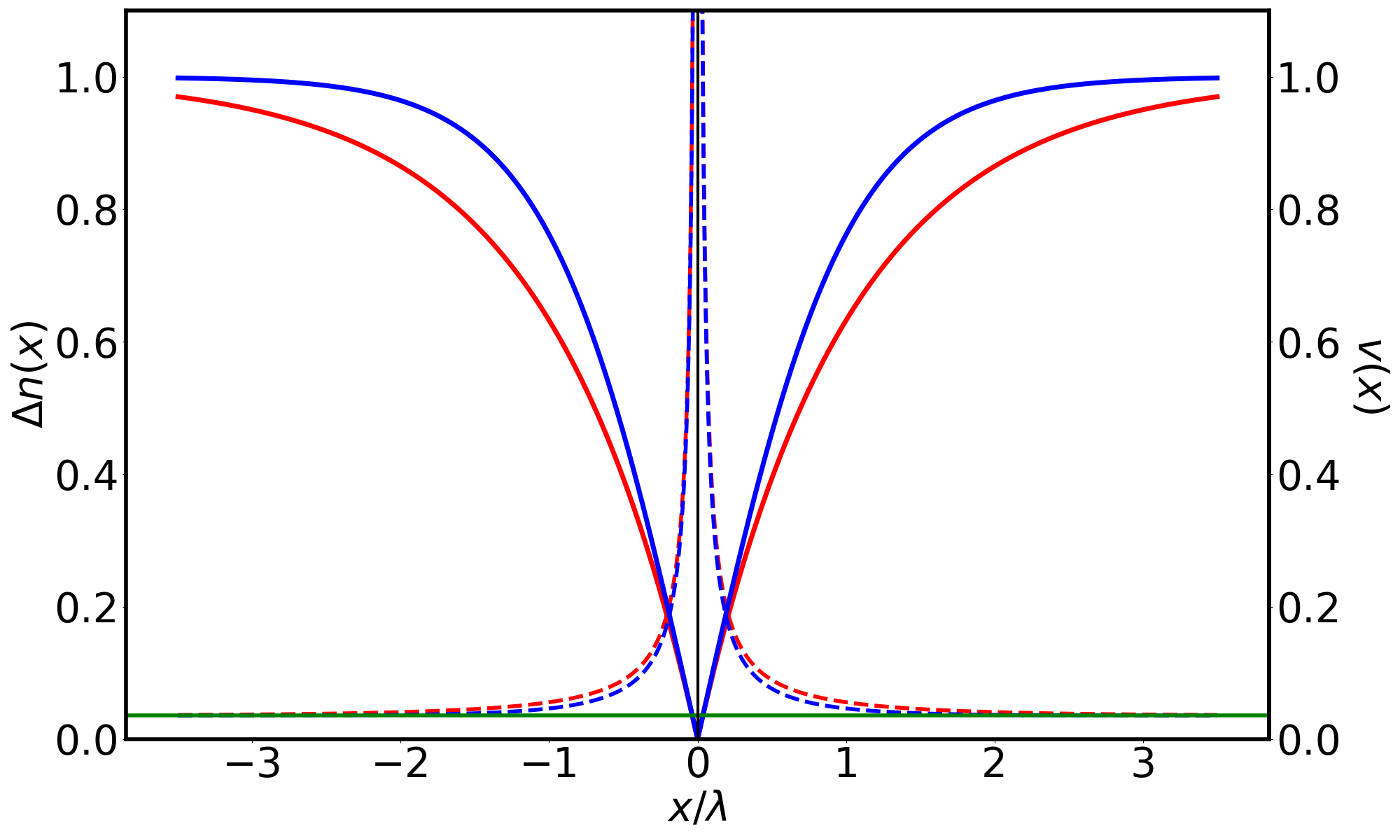
Figure 1: The solid curves show the normalized inhomogeneous velocity profiles for a 1D Dirac system, $v(x)\propto\tanh|x|/\lambda$ (tanh case, upper blue curve), and $v(x)\propto(1-{\rm e}^{-|x|/\lambda})$ (sigmoid case, lower red curve) and characterized by a length scale $\lambda$. The dashed curves show the predicted local densities of positive-energy fermions induced after a sudden quench from the homogeneous velocity case to the inhomogeneous profile, representing an analog Unruh effect. Here the upper red dashed curve (lower blue dashed curve) corresponds to the sigmoid (tanh) cases, with the green curve being the asymptotic value at large $|x|$.

To achieve an analog Unruh effect in a lab setting, it is not necessary to engineer an accelerating Rindler observer. Rather, a simpler strategy is exploit the fact that a coordinate change transforms the Rindler metric to that of a spacetime with a spatially-varying speed of light, of the form $v(x)\propto|x|$, which plays the role of the Rindler observer in the analog setup (as we show below). However, this leads to additional difficulties, since it is challenging to realize a lab-based system described by a Dirac equation with $v(x)\propto|x|$ for all $x$. For example, it is well-known that graphene-like systems with spatially-varying nearest-neighbor tunneling (realizable with a spatially-varying imposed strain deJuan:2012hxm or with an appropriately engineered light field Jimenez-Galan:2020 ) can yield a spatially varying velocity. However, it is difficult to see how such approaches can lead to $v(x)\propto|x|$ for all $x$ (a highly nonperturbative change in the local Dirac velocity).

A natural next question, to be addressed here, is to what extent an approximate analog Unruh effect can be realized in a Dirac-type fermion system with a more realistic localized velocity profile, such as $v(x)=v\tanh(|x|/\lambda)$. Such a velocity profile, illustrated as the solid (upper) blue line in Fig. 1, exhibits $v(x)\propto|x|$ for $|x|\ll\lambda$, with $\lambda$ a length scale characterizing the size of the distortion. For $|x|\gg\lambda$, we have $v(x)=v$, the background velocity in the absence of the applied strain. Although easier to realize in an experiment, such a velocity profile can only yield an approximate Unruh effect, since the mapping to a uniformly accelerating observer no longer holds. Despite this, we find the approximate Unruh effect to still be characterized by the same Unruh temperature as the strictly linear case $v(x)\propto|x|$. We find that the positive-energy fermions associated with this approximate emergent Unruh effect are spatially localized near $x=0$, as seen in the dashed lines of Fig. 1.

This paper is organized as follows. In Sec. II we describe our model Hamiltonian for a 1D Dirac system with an inhomogeneous local Dirac velocity and review the system ground state for the well-known case of a uniform velocity. In Sec. III we review how a quench from an initial uniform-velocity case to the linear velocity case $v(x)\propto|x|$ yields the Unruh effect: an emergent Fermi distribution of particles despite the physical system being at zero temperature. In Sec. IV, we generalize these calculations to the case of the nonlinear velocity profiles shown in Fig. 1, finding an approximate Unruh effect still emerges in this case. In Sec. V, we study the spatial distribution of positive-energy fermions associated with this Unruh effect, showing the spatial distributions given by the dashed cuves in Fig. 1. In Sec. VI we provide brief concluding remarks and discuss future directions for study.

II Model Hamiltonian

Following the approach of Ref. Bhardwaj2023 , which analyzed the Unruh effect for 2D Dirac systems with a spatially-varying velocity, here we analyze a 1D version with Hamiltonian

$$H=\sqrt{v(x)}\sigma_{x}p_{x}\sqrt{v(x)},$$ (1)

where $p_{x}=-i\hbar\partial_{x}$ is the usual $x$-momentum operator and $\sigma_{x}=\big{(}\begin{smallmatrix}0&1\\ 1&0\end{smallmatrix}\big{)}$ is the Pauli matrix. We note that, as written, the Hamiltonian in Eq. (1) is Hermitian, and that below Planck’s constant $\hbar$ will generally be set to unity. Before proceeding, we remark that inhomogeneous Dirac systems like Eq. (1) have been studied in other contexts, for example Refs. Ghorashi:2020 ; Davis:2022 that studied analog gravitational lensing and Ref. Morice2022 that studied quantum dynamics in lattice models that realize Hamiltonians like Eq. (1).

Our first task is to recall the case of a spatially-uniform velocity, $v(x)=v$. In this case, Eq. (1) is a model for 1D Dirac Fermions with eigenfunctions $\hat{\psi}_{p\alpha}(x)=\hat{\chi}_{\alpha}{\rm e}^{ipx}$ and energies $E_{\alpha}(p)=\alpha vp$ where $\alpha=\pm$. Here and below hatted quantities denote two-component spinors with components labeled by $i,j$. The spinors $\hat{\chi}_{\alpha}$ are just the eigenspinors of $\sigma_{x}$, explicitly given by $\hat{\chi}_{+}=\frac{1}{\sqrt{2}}\big{(}\begin{smallmatrix}1\\ 1\end{smallmatrix}\big{)}$ and $\hat{\chi}_{-}=\frac{1}{\sqrt{2}}\big{(}\begin{smallmatrix}1\\ -1\end{smallmatrix}\big{)}$.

Turning to the many-body case with spinless fermions, we define two-component real-space field operators $\hat{\Psi}(x)$ obeying the anticommutator relation

$$\{\Psi_{i}(x),\Psi_{j}^{\dagger}(x^{\prime})\}=\delta_{ij}\delta(x-x^{\prime}).$$ (2)

To describe the system ground state and excitations, we define mode operators $c_{p\alpha}$ ($c_{p\alpha}^{\dagger}$) that annihilate (create) particles in the single-particle state $\hat{\psi}_{p\alpha}$. These operators obey the anticommutator relation

$$\{c_{p\alpha}^{\phantom{\dagger}},c_{p^{\prime}\beta}^{\dagger}\}=2\pi\delta_{\alpha\beta}\delta(p-p^{\prime}).$$ (3)

The field and mode operators are connected by the relations

$$\hat{\Psi}(x) = \sum_{\alpha=\pm}\int_{-\infty}^{\infty}\frac{dp}{2\pi}\,\hat{\psi}_{p\alpha}(x)c_{p\alpha},$$ (4)

$$c_{p\alpha} = \int_{-\infty}^{\infty}dx\,\hat{\psi}^{\dagger}_{p\alpha}(x)\hat{\Psi}(x),$$ (5)

Having defined the relevant quantum field and mode operators, next we define the system ground state (the analog Minkowski vacuum), in which all negative (positive) energy states have unit (vanishing) occupation. This is captured by the expectation value (EV):

$$\langle c_{p\alpha}^{\dagger}c_{p^{\prime}\beta}^{\phantom{\dagger}}\rangle=2\pi\delta_{\alpha\beta}\Theta(-\alpha p)\delta(p-p^{\prime}).$$ (6)

The Unruh effect emerges when the Minkowski state is “observed” by the Rindler system, which consist of Dirac fermions in the presence of an engineered velocity profile $v(x)$.

The proposed experimental procedure to realize this is as follows Bhardwaj2023 : A system of Dirac fermions obeying Eq. (1) is prepared in the Minkowski vacuum Eq. (6). Subsequently, a rapid quench to the engineered profile $v(x)$ is induced, for example by imposing a strain deJuan:2012hxm or an external light field Jimenez-Galan:2020 , which can modify the hopping matrix elements of an underlying tight-binding model and hence the local velocity. Within the sudden approximation of quantum mechanics, observables in the final system are computed by taking the EV of the corresponding operators with respect to the initial (pre-quench) state, i.e., the Minkowksi vacuum. The emergent Unruh effect reflects the fact that this final EV describes spontaneous particle creation, as we shall see.

Having defined the initial Minkowski state in this section, our next task is to analyze possible final states, described by a Dirac equation with a spatially-inhomogeneous velocity profile.

III Linear Velocity Profile: Ideal Unruh effect

As we have discussed, our aim is to investigate the emergence of the Unruh effect in a simple 1D Dirac model with a spatially-varying velocity $v(x)$. In particular, we are interested in how the associated particle creation depends on the details of $v(x)$. In this section, we study the case of a linear velocity profile, $v(x)=v|x|/\lambda$. We emphasize that such a linear profile corresponds, in the analogy to the conventional Unruh effect, to a uniformly accelerating Rindler observer. Thus, we expect (and indeed find) an exact Unruh effect in this case. This case will serve as a basis for what to expect for the subsequent velocity profiles, discussed below.

To demonstrate the Unruh effect in this system, we first compute the eigenfunctions of $H$, Eq. (1), for the present velocity profile. The corresponding Hamiltonian is:

$$H=\frac{v}{\lambda}\sqrt{|x|}\sigma_{x}(-i\hbar\partial_{x})\sqrt{|x|},$$ (7)

with $\lambda$ a length scale associated with the spatial variation of the velocity profile. At this point we set $\lambda=1$, $v=1$ and $\hbar=1$ for simplicity, restoring them at the end of the section.

A key property of this particular Hamiltonian is the disjunction at $x=0$, thus rendering a spatially inhomogenous differential equation. This means we can treat the solutions as referring to their own half-space, separately considering $x>0$ and $x<0$. Focusing on $x>0$ (indicated with a subscript $>$), we find the eigenfunctions (with eigenvalue $E$)

$$\hat{\psi}_{>E\alpha}(x)=\frac{1}{\sqrt{2\pi x}}{\rm e}^{\alpha iE\ln x}\hat{\chi}_{\alpha},$$ (8)

which satisfy orthonormality and completeness relations:

$$\int_{0}^{\infty}dx\,\hat{\psi}_{>E\alpha}^{\dagger}(x)\hat{\psi}_{>E^{\prime}\beta}(x)=\delta_{\alpha\beta}\delta(E-E^{\prime}),$$ (9)

$$\sum_{\alpha=\pm}\int_{-\infty}^{\infty}dE\,\hat{\psi}_{>E\alpha}(x)\hat{\psi}_{>E\alpha}^{\dagger}(x^{\prime})=\delta(x-x^{\prime})\mathbb{1},$$ (10)

where $\mathbb{1}$ is the unit matrix in the two component space of eigenfunctions of $H$.

As in the uniform $v$ case, to study a many-body system of fermions described by the Hamiltonian Eq. 7 we introduce “final” mode operators $d_{>E\alpha}^{\phantom{\dagger}}$ ($d_{>E\alpha}^{\dagger}$) that annihilate (create) fermions in the state with energy $E$ and band index $\alpha$ in the $x>0$ region. Then, operators corresponding to observables in the final system can be built from these mode operators. To apply the sudden approximation as described above, in which any EVs should be computed with respect to the initial ground state, we must find a relation between the final ($d_{>E\alpha}^{\phantom{\dagger}}$) and initial ($c_{p\alpha}^{\phantom{\dagger}}$) mode operators. To achieve this, we first express the real-space field operator (for $x>0$) in terms of the final mode operators:

$$\hat{\Psi}(x)=\sum_{\alpha=\pm}\int_{-\infty}^{\infty}dE\hat{\psi}_{>E\alpha}(x)d_{>E\alpha}.$$ (11)

With this definition, the anti-commutation relation $\{d_{>E_{1}\alpha},d_{>E_{2}\beta}^{\dagger}\}=\delta(E_{1}-E_{2})\delta_{\alpha\beta}$ is consistent with the real-space anti-commutator relation for the field operators in Eq. (2). The inverse relation to Eq. (11) is

$$d_{>E\alpha}=\int_{0}^{\infty}dx\,\hat{\psi}_{>E\alpha}^{\dagger}\hat{\Psi}(x).$$ (12)

Now, to achieve the desired expression of the $d_{>E\alpha}$ in terms of the $c_{p\alpha}$ we just need to insert Eq. (4) into the right side of Eq. (12) and evalute the resulting $x$ integral. We get:

$$d^{{\phantom{\dagger}}}_{>E\alpha}\!\! = \!\!\sum_{\beta=\pm}\int_{-\infty}^{\infty}\frac{dp}{2\pi}\int^{\infty}_{0}dx\,\psi^{\dagger}_{>E\alpha}(x)\psi^{{\phantom{\dagger}}}_{p\beta}(x)c^{{\phantom{\dagger}}}_{p\beta},$$ (13)

$$= \int_{-\infty}^{\infty}\frac{dp}{2\pi}X^{{\phantom{\dagger}}}_{\alpha}(p,E)c^{{\phantom{\dagger}}}_{p\alpha},$$ (14)

where the function $X_{\alpha}^{{\phantom{\dagger}}}$ comes from the inner product of the strained and unstrained eigenfunctions and is given by:

$$X^{{\phantom{\dagger}}}_{\alpha}(p,E)=\int_{0}^{\infty}dx\frac{1}{\sqrt{2\pi x}}{\rm e}^{-i\alpha E\ln x}{\rm e}^{ipx},$$ (15)

$$=\frac{1}{\sqrt{2\pi|p|}}{\rm e}^{i\alpha E\ln|p|}{\rm e}^{i\frac{\pi}{4}{\rm sgn}(p)}{\rm e}^{{\rm sgn}(p)\alpha E\pi/2}\Gamma\Big{[}\frac{1}{2}-i\alpha E\Big{]},$$

with $\Gamma(z)$ the gamma function. Then, given an initial state in terms of the $c_{p\alpha}$ (e.g., a vacuum or thermal state), Eq. (14) allows us to evaluate EVs of the final system in terms of the initial EV. For example, consider the $+$ band average

$$\langle d_{>E_{1}+}^{\dagger}d_{>E_{2}+}^{{\phantom{\dagger}}}\rangle$$ (16)

$$=\int_{-\infty}^{\infty}\frac{dp}{2\pi}X^{*}_{+}(p,E_{1})\int_{-\infty}^{\infty}\frac{dp^{\prime}}{2\pi}X^{{\phantom{\dagger}}}_{+}(p^{\prime},E_{2})\langle c^{\dagger}_{p+},c^{{\phantom{\dagger}}}_{p^{\prime}+}\rangle.$$

If we assume the Minkowski vacuum initial state, then the EV on the right is given by Eq. (6) above. Since we’re studying the $\alpha=+$ case, with the $p<0$ states occupied and $p>0$ states empty, we get:

$$\langle d_{>E_{1}+}^{\dagger}d_{>E_{2}+}^{{\phantom{\dagger}}}\rangle = \int_{-\infty}^{0}\frac{dp}{2\pi}X_{+}^{*}(p,E_{1})X_{+}(p,E_{2})$$ (17)

$$= \delta(E_{1}-E_{2})\frac{1}{{\rm e}^{2\pi E_{1}}+1},$$ (18)

i.e., a Fermi distribution at “temperature” $1/(2\pi)$. Following the same steps for the $-$ band we get:

$$\langle d^{\dagger}_{>E_{1}-}d_{>E_{2}-}\rangle = \int_{0}^{\infty}\frac{dp}{2\pi}X_{-}^{*}(p,E_{1})X_{-}(p,E_{2}),$$ (19)

$$= \delta(E_{1}-E_{2})\frac{1}{{\rm e}^{2\pi E_{1}}+1},$$ (20)

the same final result again reflecting a Fermi distribution. Taking these results together, and reintroducing dimensionful parameters, we obtain (defining the Fermi distribution $n_{\rm F}(E,T)=\frac{1}{{\rm e}^{E/(k_{\rm B}T)}+1}$):

$$\langle d_{>E_{1}\alpha}^{\dagger}d^{{\phantom{\dagger}}}_{>E_{2}\beta}\rangle=\delta_{\alpha\beta}n_{\rm F}(E_{1},T_{\rm U})\delta(E_{1}-E_{2}),$$ (21)

thereby recovering the well-known Unruh effect (also known as the Fulling-Davies-Unruh effect Fulling:1972md ; Davies:1974th ; Unruh:1976db ), with the final Unruh temperature (restoring $v$, $\lambda$ and $\hbar$ that were previously set to unity):

$$T_{\rm U}=\frac{v\hbar}{2\pi\lambda k_{\rm B}}.$$ (22)

Within this analog Unruh effect, the role of “acceleration” is determined by the ratio $a=c^{2}/\lambda$, as can be seen by comparing to the conventional Unruh temperature $T_{\text{U}}=\frac{\hbar a}{2\pi k_{\text{B}}c}$ and identifying $v=c$.

Here we make a technical remark that the final integrals in Eqs. (17) and (19) can be most easily evaluated by using the integral representation of the function $X_{\alpha}(p,E)$ in the first line of Eq. (15) and evaluating the $p$ integrals first. In the next section, in which we study alternate velocity profiles $v(x)$, we will follow this strategy.

The results of this section confirm that an analog Unruh effect can emerge in a 1D Dirac model under the condition of a sudden quench of the velocity profile from a uniform homogeneous velocity $v(x)=v$ to a highly inhomogeneous velocity profile $v(x)=v|x|/\lambda$. Our next task is to study alternate velocity profiles in which the modification of the velocity is spatially localized.

IV Nonlinear velocity profile

As we have seen, the linear case gave the expected perfect Unruh effect, with the occupation of states of the final system being given by a Fermi distribution. However, it may be difficult in a real experiment to realize the required perfect linear velocity profile for all $x$. To investigate this, in this section we consider nonlinear velocity profiles after the quench, starting with a “sigmoid” velocity profile followed by a “tanh” velocity profile, which will yield qualitatively similar results.

IV.1 Sigmoid velocity profile

The sigmoid velocity profile we study takes the form:

$$v(x)=v\big{(}1-{\rm e}^{-|x|/\lambda}\big{)}.$$ (23)

going as $|x|$ for $x\to 0$ but constant at large $|x|\gg\lambda$, with $\lambda$ a length scale characterizing the size of the deformation. Once again, we take $v,\lambda\to 1$ for simplicity, only reintroducing them in final results. Since $v(x)$ is only significantly modified near $x=0$, achieving this case in an experiment is expected to be easier than in the $v(x)\propto|x|$ case.

As in the preceding section, we need the eigenfunctions of the single-particle Hamiltonian corresponding to $v(x)$ in Eq. (23):

$$H=\sqrt{1-e^{-|x|}}{(-i\partial_{x})}\sqrt{1-e^{-|x|}}.$$ (24)

It is sufficient to focus on $x>0$. We find the eigenfunctions

$$\hat{\psi}_{>E\alpha}(x)=\frac{1}{\sqrt{2\pi}}{\rm e}^{\frac{1}{2}x}\big{(}{\rm e}^{x}-1\big{)}^{i\alpha E-\frac{1}{2}}\hat{\chi}_{\alpha},$$ (25)

that are orthonormal and complete in the region $x>0$. As previously, to investigate the Unruh effect we express the real-space field operators in terms of mode operators (again called $d_{>E\alpha}^{\phantom{\dagger}}$ and $d_{>E\alpha}^{\dagger}$). These operators can again be connected to the initial mode operators via an expression of the form of Eq. (14) but with a different function $X_{\alpha}(p,E)$. Although we can find an explicit expression for the corresponding function, it is easier to work with an integral representation when evaluating the number operator in the present case.

We focus on the $\alpha=+$ band with similar results holding for the $-$ case. Following similar steps to the previous section (assuming the initial system EV given by Eq. (6)), we find:

$$\langle d_{>E_{1}+}^{\dagger}d_{>E_{2}+}\rangle=\int_{-\infty}^{0}\frac{dp}{(2\pi)^{2}}\int_{0}^{\infty}dx_{1}{\rm e}^{\frac{1}{2}x_{1}}\big{(}{\rm e}^{x_{1}}-1\big{)}^{iE_{1}-\frac{1}{2}}$$

$$\qquad\times\int_{0}^{\infty}dx_{2}{\rm e}^{\frac{1}{2}x_{2}}\big{(}{\rm e}^{x_{2}}-1\big{)}^{-iE_{2}-\frac{1}{2}}{\rm e}^{-ip(x_{1}-x_{2})},$$ (26)

for the expectaton value of the final system mode operators.

As mentioned above, we find it advantageous to first evaluate the $p$ integral, which we interpret in the sense of a distribution using:

$$\int_{-\infty}^{0}\frac{dp}{2\pi}{\rm e}^{-ip(x_{1}-x_{2})}={\rm Lim.}_{\eta\to 0+}\int_{-\infty}^{0}\frac{dp}{2\pi}{\rm e}^{-ip(x_{1}-x_{2})}{\rm e}^{\eta p}$$

$$\qquad\qquad={\rm Lim.}_{\eta\to 0+}\frac{1}{2\pi}\frac{1}{\eta-i(x_{1}-x_{2})}$$ (27)

$$\qquad\qquad=\frac{i}{2\pi}\Big{(}{\cal P}\frac{1}{x_{1}-x_{2}}-i\pi\delta(x_{1}-x_{2})\Big{)},$$ (28)

with ${\cal P}$ indicating principal value and where we have used the Sokhotski-Plemelj formula. Upon plugging this in to Eq. (26), the contribution from the delta function will pin $x_{2}=x_{1}$. Dropping the subscript, the resulting $x$ integral gives an energy delta function:

$$\frac{1}{2\pi}\int_{0}^{\infty}dx\,{\rm e}^{x}\Big{(}{\rm e}^{x}-1\Big{)}^{i(E_{1}-E_{2})-1}=\delta(E_{1}-E_{2}),$$ (29)

which is easiest to check by changing variables to $y=\ln\big{[}{\rm e}^{x}-1\big{]}$, leading to the well-known delta-function representation

$$\int_{-\infty}^{\infty}\frac{dy}{2\pi}{\rm e}^{iy(E_{1}-E_{2})}=\delta(E_{1}-E_{2}).$$ (30)

The formula Eq. (29) that simplified the delta-function contribution to Eq. (26) is in fact a re-statement of the orthonormality of the system eigenfunctions Eq. (25). Including the contribution from the principal value term in Eq. (28), we have

$$\langle d^{\dagger}_{>E_{1}+}d_{>E_{2}+}^{{\phantom{\dagger}}}\rangle=\frac{1}{2\pi}\big{(}\frac{1}{2}\delta(E^{{\phantom{\dagger}}}_{1}-E^{{\phantom{\dagger}}}_{2})+\mathfrak{R}(E^{{\phantom{\dagger}}}_{1},E^{{\phantom{\dagger}}}_{2})\big{)},$$ (31)

where the second term in parentheses is:

$$\mathfrak{R}(E_{1},E_{2})=\frac{i}{4\pi^{2}}\int_{0}^{\infty}dx_{1}\,{\rm e}^{\frac{1}{2}x_{1}}\big{(}{\rm e}^{x_{1}}-1\big{)}^{iE_{1}-\frac{1}{2}}$$

$$\times\int_{0}^{\infty}dx_{2}\,{\rm e}^{\frac{1}{2}x_{2}}\big{(}{\rm e}^{x_{2}}-1\big{)}^{-iE_{2}-\frac{1}{2}}{\cal P}\frac{1}{x_{1}-x_{2}}.$$ (32)

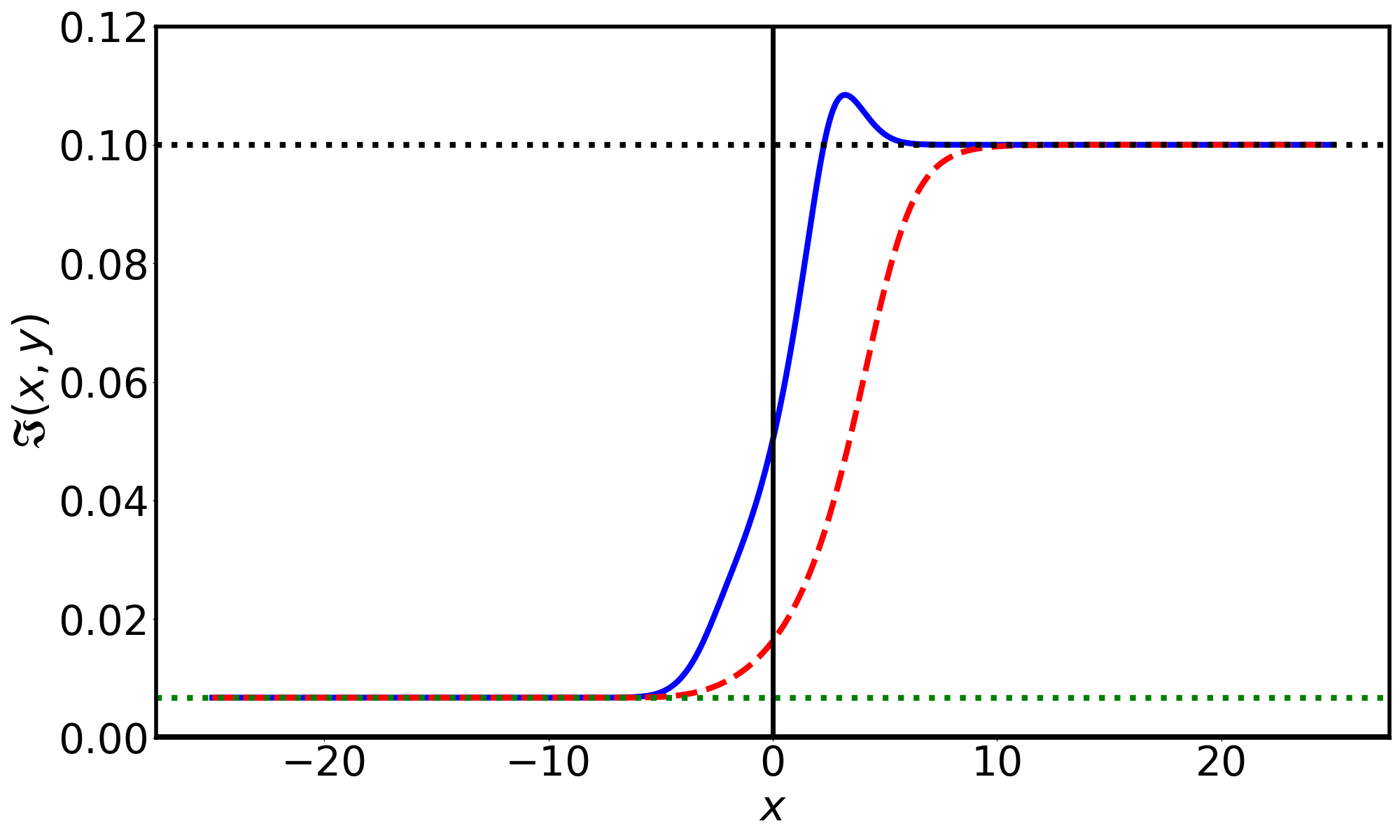
Figure 2: Plots of the integrand $\mathfrak{I}(x,y)$ in the sigmoid case Eq. (35) (red dashed) and in the hyperbolic tangent case Eq. (45) (solid blue) for the case $y=10$, showing that this function rapidly reaches the asymptotic behavior given by Eq. (36). To illustrate these limits, the top black dotted line is at $1/y=0.1$ and the bottom green dotted line is at $1/(2\sinh(y/2))\simeq 0.0067$.

To study the contribution due to $\mathfrak{R}(E_{1},E_{2})$, we make a variable change:

$$x^{{\phantom{\dagger}}}_{1}=\ln(e^{{x}+y/2}+1),x^{{\phantom{\dagger}}}_{2}=\ln(e^{{x}-y/2}+1).$$ (33)

The resulting Eq. (32) becomes:

$$\mathfrak{R}(E_{1},E_{2})$$ (34)

$$=\frac{i}{4\pi^{2}}\int_{-\infty}^{\infty}dx\int_{-\infty}^{\infty}dy\,\mathfrak{I}(x,y)e^{i(E_{1}-E_{2})x}e^{\frac{i}{2}(E_{1}+E_{2})y}.$$

where the integrand $\mathfrak{I}(x,y)$ is given by:

$$\mathfrak{I}(x,y)\!=\!\sqrt{\frac{e^{x}}{2(\cosh x\!+\!\cosh(y/2))}}{\cal P}\frac{1}{\ln\left(\frac{e^{x+y/2}+1}{e^{x-y/2}+1}\right)}.$$ (35)

Although the remaining integrals are too difficult to evaluate directly, we can make a simple approximation by noting that, as a function of $x$, $\mathfrak{I}(x,y)$ rapidly reaches an asymptotic $y$-dependent value for $x\to\pm\infty$. Indeed, we find the limiting behavior

$$\mathfrak{I}(x,y)=\begin{cases}\frac{1}{y},&\text{for $x\to+\infty$,}\cr\frac{1}{2\sinh(y/2)}&\text{for $x\to-\infty$.}\end{cases}$$ (36)

This limiting behavior is easily verified by plotting this function, as we do in Fig. 2, for the present case and also for the case of the hyperbolic tangent velocity profile discussed below. This figure shows that these limits are reached very rapidly as a function of $x$, approximately justifying our replacement of $\mathfrak{I}(x,y)$ by its limiting values for $x>0$ and $x<0$. Defining the average energy $\bar{E}=(E_{1}+E_{2})/2$, this approximation leads to:

$$\mathfrak{R}(E_{1},E_{2})\simeq-\frac{1}{4\pi^{2}}\int^{0}_{-\infty}dx{\rm e}^{i(E_{1}-E_{2})x}\int^{\infty}_{-\infty}\frac{dy}{y}\sin(y\bar{E})$$

$$-\frac{1}{4\pi^{2}}\int^{\infty}_{0}dx{\rm e}^{i(E_{1}-E_{2})x}\int^{\infty}_{-\infty}dy\frac{\sin(y\bar{E})}{2\sinh(y/2)}.$$ (37)

In this expression we also took into account the fact that $\mathfrak{I}(x,y)$ is odd in $y$.

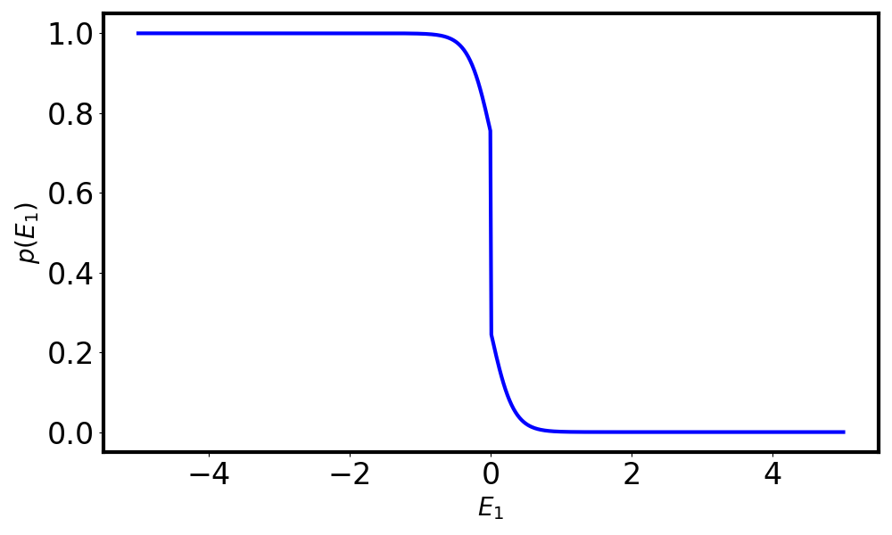
Figure 3: Plot of the occupation of levels near the Fermi surface, $p(E_{1})$, showing the approximate Unruh effect, with a depletion of negative energy states and an increase of positive energy states. Here, $E_{1}$ is the energy normalized to $k_{\rm B}T_{\rm U}$ with the Unruh temperature given above in Eq. (22).

After evaluating the remaining integrals, we arrive at

$$\mathfrak{R}(E_{1},E_{2})\simeq-\frac{1}{4}\Big{[}{\rm sgn}(\bar{E})+\tanh(\pi\bar{E})\Big{]}\delta(E_{1}-E_{2})$$

$$\qquad\qquad+\frac{i}{4\pi}\Big{[}{\rm sgn}(\bar{E})-\tanh(\pi\bar{E})\Big{]}{\cal P}\frac{1}{E_{1}-E_{2}}.$$ (38)

Upon combining this with Eq. (31) we get

$$\langle d_{>E_{1}+}^{\dagger}d_{>E_{2}+}\rangle=\delta(E_{1}-E_{2})p(E_{1})$$

$$+\frac{i}{4\pi}\Big{[}{\rm sgn}(\bar{E})-\tanh(\pi\bar{E})\Big{]}{\cal P}\frac{1}{E_{1}-E_{2}},$$ (39)

where the prefactor in the first term is equal to

$$p(E_{1}) = \frac{1}{2}-\frac{1}{4}{\rm sgn}(E_{1})-\frac{1}{4}\tanh(\pi E_{1})$$ (40)

$$= \begin{cases}\frac{1}{2}n_{\rm F}(E_{1},T_{\rm U}),&\text{for $E_{1}>0$,}\cr 1-\frac{1}{2}n_{\rm F}(-E_{1},T_{\rm U}),&\text{for $E_{1}<0$,}\end{cases}$$

where in the second line we reintroduced dimensionful quantities that were previously set to unity, to show that the function $p(E_{1})$ (that is approximately the fermion occupation at energy $E_{1}$) after the quench is indeed characterized by the Unruh temperature $T_{\rm U}$ defined in Eq. (22).

We see that, while the sigmoid velocity profile does not lead to an exact Unruh effect, we do see a modified Unruh effect if we can regard the first term of Eq. (39) as being dominant (this is reasonable since it is proportional to an energy delta function) and if the approximations leading to this result are valid. The function $p(E_{1})$, plotted in Fig. 3, shows a creation of particles for $E_{1}>0$ and depletion of particles (or creation of holes) for $E_{1}<0$. This is qualitatively consistent with the exact Unruh effect (although reduced in magnitude). We emphasize that this is not a true thermal state, since the system is still in the zero temperature Minkoswki vacuum.

IV.2 Hyperbolic Tangent Profile

In this section we repeat the preceding calculations for a velocity profile that is qualitatively similar to the sigmoid case, which is the hyperbolic tangent (tanh) velocity function:

$$v(x)=v\tanh\left(\frac{|x|}{\lambda}\right).$$ (41)

The corresponding single-particle Hamiltonian is (taking $v=\lambda=\hbar=1$ as previously):

$$H=\sqrt{\tanh|x|}{(-i\partial_{x})}\sqrt{\tanh|x|}.$$ (42)

Focusing on $x>0$, we find the eigenfunctions at energy $E$ to be:

$$\psi^{{\phantom{\dagger}}}_{>E\alpha}(x)=\sqrt{\frac{\coth(x)}{2\pi}}e^{\alpha iE\ln(\sinh(x))}\hat{\chi}^{{\phantom{\dagger}}}_{\alpha}$$ (43)

For this profile, we also found the approach of evaluating the momentum integral first to assist in simplifying the analysis. Indeed, it turns out the steps are almost identical to the sigmoid case, also leading to Eq. (31) with the function $\mathfrak{R}(E_{1},E_{2})$ still given by Eq. (34) but with a different integrand $\mathfrak{I}(x,y)$ arising after the variable change

$$x^{{\phantom{\dagger}}}_{1}=\sinh^{-1}(e^{x+y/2}),x^{{\phantom{\dagger}}}_{2}=\sinh^{-1}(e^{x-y/2}).$$ (44)

The explicit form for $\mathfrak{I}(x,y)$ in the tanh case is:

$$\mathfrak{I}(x,y)=\frac{e^{x/2}}{(2[\cosh(2x)+\cosh(y/2)])^{1/4}}$$

$$\qquad\qquad\times{\cal P}\frac{1}{\ln\left(\frac{\sqrt{e^{y}+e^{-2x}}+e^{y/2}}{\sqrt{e^{-y}+e^{-2x}}+e^{-y/2}}\right)}.$$ (45)

Although this function is different from the sigmoid case, the limiting behavior as a function of $x$ (at fixed $y$) is identical, again given by Eq. (36) as illustrated by the solid blue curve of Fig. 2. Thus, a sudden quench to the tanh profile gives (within the same approximation) the same result Eq. (39), with the approximate occupation $p(E_{1})$ again given by Eq. (40).

Having established an approximate Unruh effect within two similar models of the post-quench velocity profile, in the next section we study the real-space spatial extent of the emergent Unruh particles.

V Spatial extent of the Unruh effect

We have seen that a quench to an inhomogeneous velocity profile that is linear at small $|x|\ll\lambda$ and constant at large $|x|\gg\lambda$ leads to an approximate Unruh effect characterized by the creation of positive energy electrons and of negative energy holes that looks approximately like a thermal state. To gain additional insight into this state, in this section we study the spatial extent (or local density) of the induced positive energy fermions.

We define the local density of positive energy fermions:

$$\Delta n(x)=\sum_{\alpha,\beta}\int_{0}^{\infty}dE_{1}\int_{0}^{\infty}dE_{2}\hat{\psi}^{\dagger}_{>E_{1}\alpha}(x)\hat{\psi}^{{\phantom{\dagger}}}_{>E_{2}\beta}(x)$$

$$\qquad\qquad\qquad\qquad\times\langle d^{\dagger}_{>E_{1}\alpha}d_{>E_{2}\beta}^{{\phantom{\dagger}}}\rangle.$$ (46)

Plugging in our result for the final occupation Eq. (39) that applies to both cases, we find the contribution due to the second line vanishes, leaving

$$\Delta n(x)=\sum_{\alpha=\pm}\int_{0}^{\infty}dE\hat{\psi}^{\dagger}_{>E\alpha}(x)\hat{\psi}^{{\phantom{\dagger}}}_{>E\alpha}(x)\frac{1}{2}n_{\rm F}(E,T_{U}).$$ (47)

Interestingly, the product of wavefunctions in the integrand of this expression is, generally, simply proportional to $1/v(x)$. To see this, we note that eigenfunctions for Eq. (1) take the form (with $\hbar=1$):

$$\hat{\psi}_{>E\alpha}(x)=\hat{\chi}_{\alpha}\frac{c}{\sqrt{v(x)}}{\rm e}^{i\alpha E\int_{x_{0}}^{x}dx^{\prime}\frac{1}{v(x^{\prime})}},$$ (48)

with $x_{0}$ an arbitrary initial position and $c$ a normalization factor (equal to $1/\sqrt{2\pi}$ in both cases), immediately implying

$$\Delta n(x)=\frac{|c|^{2}}{v(x)}\int_{0}^{\infty}dEn_{\rm F}(E,T_{U})=\frac{|c|^{2}}{v(x)}k_{\rm B}T_{U}\ln 2.$$ (49)

This result (plotted as dashed curves in Fig. 1, with dimensionful quantities set to unity) shows that the positive-energy fermions (i.e., the $E_{1}>0$ regime of Fig. 3) emerging from the approximate Unruh effect induced by a spatially-varying velocity $v(x)$ are localized, spatially, near $x=0$ where $v(x)\to 0$. The $E_{1}<0$ regime of Fig. 3) shows a similar depletion of fermions for negative energies; these will give a local density change that is exactly the opposite of Eq. (49). Although the total local charge density is therefore unchanged, the energy dependence can likely be probed by energy-sensitive probes like scanning tunneling microscopy. We leave the investigation of further experimental probes of this state for future work.

VI Concluding Remarks

We have studied the Unruh effect in a model of one-dimensional Dirac fermions with a controllable local Dirac velocity $v(x)$ that (by assumption) can be spatially uniform or spatially nonuniform. The uniform case $v$ case corresponds to a conventional theory of 1D Dirac fermions, with a “Minkowski” vacuum ground state.

The Unruh effect occurs after a sudden quench to an inhomogeneous velocity profile, with the system occupation characterized by an Fermi distribution with an emergent temperature $T_{\rm U}$. After first studying the ideal case with $v(x)\propto|x|$ (in which the final system is connected to Dirac fermions in Rindler spacetime), we turned to the case of more experimentally-realizable velocity profiles that are linear at small $|x|$ and homogeneous for large $|x|$ (beyond a length scale $\lambda$). The latter cases led to an approximate Unruh effect, with a distribution of fermions also characterized by a Fermi distribution. As a signature of this approximate Unruh effect, we studied the spatial profile, as a function of position, of the number of positive-energy excitations, finding it to be localized near $x=0$ with a profile proportional to the reciprocal of the final velocity profile.

Our work shows that the physics of the Unruh effect can emerge in condensed matter systems that only approximately realize the conditions of an ideal Unruh effect. Future possible directions for study include computing other observables (including transport and thermodynamic properties as well as probes like tunneling and photoemission), generalizing to the case of a finite temperature initial state, and studying the predicted statistics inversion of the Unruh effect Takagi ; Ooguri that is connected to Huygens’ principle for wave motion.

VII Acknowledgments

DES acknowledges support from the National Science Foundation under Grant PHY-2208036. DES performed part of this work at the Aspen Center for Physics, which is supported by National Science Foundation grant PHY-2210452.

References

- (1) W. G. Unruh, Experimental black hole evaporation, Phys. Rev. Lett. 46, 1351 (1981).
- (2) C. Barcelo, S. Liberati and M. Visser, Analogue gravity, Living Rev. Rel. 14, 3 (2011).
- (3) P. D. Nation, J. R. Johansson, M. P. Blencowe and F. Nori, Stimulating Uncertainty: Amplifying the Quantum Vacuum with Superconducting Circuits, Rev. Mod. Phys. 84, 1 (2012).
- (4) M.J. Jacquet, S. Weinfurtner, and F. König, The next generation of analog gravity experiments, Phil. Trans. R. Soc. A. 378, 20190239 (2020).
- (5) T. G. Philbin, C. Kuklewicz, S. Robertson, S. Hill, F. Konig and U. Leonhardt, Fiber-optical analogue of the event horizon, Science 319, 1367 (2008).
- (6) F. Belgiorno et al., Hawking radiation from ultrashort laser pulse filaments, Phys. Rev. Lett. 105, 203901 (2010).
- (7) S. Weinfurtner, E. W. Tedford, M. C. J. Penrice, W. G. Unruh and G. A. Lawrence, Measurement of stimulated Hawking emission in an analogue system, Phys. Rev. Lett. 106, 021302 (2011).
- (8) J. Steinhauer, Observation of quantum Hawking radiation and its entanglement in an analogue black hole, Nature Phys. 12, 959 (2016).
- (9) U. R. Fischer and R. Schützhold, Quantum simulation of cosmic inflation in two-component Bose-Einstein condensates, Phys. Rev. A 70, 063615 (2004).
- (10) A. Prain, S. Fagnocchi and S. Liberati, Analogue Cosmological Particle Creation: Quantum Correlations in Expanding Bose Einstein Condensates, Phys. Rev. D 82, 105018 (2010).
- (11) S. Eckel, A. Kumar, T. Jacobson, I. B. Spielman and G. K. Campbell, A rapidly expanding Bose-Einstein condensate: an expanding universe in the lab, Phys. Rev. X 8, 021021 (2018).
- (12) M. Wittemer, F. Hakelberg, P. Kiefer, J.-P. Schrd̈er, C. Fey, R. Schützhold, U. Warring, and T. Schaetz, Phonon Pair Creation by Inflating Quantum Fluctuations in an Ion Trap, Phys. Rev. Lett. 123, 180502 (2019).
- (13) S. Banik, M. Gutierrez Galan, H. Sosa-Martinez, M. Anderson, S. Eckel, I. B. Spielman and G. K. Campbell, Accurate Determination of Hubble Attenuation and Amplification in Expanding and Contracting Cold-Atom Universes, Phys. Rev. Lett. 128, 090401 (2022).
- (14) J. M. Gomez Llorente and J. Plata, Expanding ring-shaped Bose-Einstein condensates as analogs of cosmological models: Analytical characterization of the inflationary dynamics, Phys. Rev. A 100, no. 4, 043613 (2019).
- (15) A. Bhardwaj, D. Vaido and D. E. Sheehy, Inflationary Dynamics and Particle Production in a Toroidal Bose-Einstein Condensate, Phys. Rev. A 103, 023322 (2021).
- (16) A. Bhardwaj, I. Agullo, D. Kranas, J.H. Wilson, and D.E. Sheehy, Entanglement in an expanding toroidal Bose-Einstein condensate, Phys. Rev. A 109, 013305 (2024).
- (17) C. Viermann, M. Sparn, N. Liebster, M. Hans, E. Kath, Á. Parra-López, M. Tolosa-Simeón, N. Sánchez-Kuntz, T. Haas and H. Strobel, et al. Quantum field simulator for dynamics in curved spacetime, Nature 611, 260 (2022).
- (18) M. Tolosa-Simeón, Á. Parra-López, N. Sánchez-Kuntz, T. Haas, C. Viermann, M. Sparn, N. Liebster, M. Hans, E. Kath and H. Strobel, et al. Curved and expanding spacetime geometries in Bose-Einstein condensates, Phys. Rev. A 106, 033313 (2022).
- (19) N. Sánchez-Kuntz, Á. Parra-López, M. Tolosa-Simeón, T. Haas, and S. Floerchinger, Scalar quantum fields in cosmologies with 2 + 1 spacetime dimensions, Phys. Rev. D. 105, 105020 (2022).
- (20) J.-C. Jaskula, G. B. Partridge, M. Bonneau, R. Lopes, J. Ruaudel, D. Boiron, and C. I. Westbrook, Acoustic Analog to the Dynamical Casimir Effect in a Bose-Einstein Condensate, Phys. Rev. Lett. 109, 220401 (2012).
- (21) C. L. Hung, V. Gurarie and C. Chin, From Cosmology to Cold Atoms: Observation of Sakharov Oscillations in Quenched Atomic Superfluids, Science 341, 1213 (2013).
- (22) A. Delhom, K. Guerrero, P.C. Calizaya, K. Falque, A. Bramati, A.J. Brady, M.J. Jacquet, and I. Agullo, Entanglement from superradiance and rotating quantum fluids of light, Phys. Rev. D 109, 105024 (2024).
- (23) S. A. Fulling, Nonuniqueness of canonical field quantization in Riemannian space-time, Phys. Rev. D 7, 2850 (1973).
- (24) P. C. W. Davies, Scalar particle production in Schwarzschild and Rindler metrics, J. Phys. A 8, 609 (1975).
- (25) W. G. Unruh, Notes on black hole evaporation, Phys. Rev. D 14, 870 (1976).
- (26) A. Retzker, J. I. Cirac, M. B. Plenio, and B. Reznik, Methods for Detecting Acceleration Radiation in a Bose-Einstein Condensate, Phys. Rev. Lett. 101, 110402 (2008).
- (27) O. Boada, A. Celi, J. I. Latorre and M. Lewenstein, Dirac Equation For Cold Atoms In Artificial Curved Spacetimes, New J. Phys. 13, 035002 (2011).
- (28) J. Rodríguez-Laguna, L. Tarruell, M. Lewenstein and A. Celi, Synthetic Unruh effect in cold atoms, Phys. Rev. A 95, 013627 (2017).
- (29) A. Kosior, M. Lewenstein and A. Celi, Unruh effect for interacting particles with ultracold atoms, SciPost Phys. 5, 061 (2018).
- (30) J. Hu, L. Feng, Z. Zhang and C. Chin, Quantum simulation of Unruh radiation, Nature Phys. 15, 785 (2019).
- (31) C. Gooding, S. Biermann, S. Erne, J. Louko, W. G. Unruh, J. Schmiedmayer and S. Weinfurtner, Interferometric Unruh detectors for Bose-Einstein condensates, Phys. Rev. Lett. 125, 213603 (2020).
- (32) A. Iorio and G. Lambiase, The Hawking-Unruh phenomenon on graphene, Phys. Lett. B 716, 334 (2012).
- (33) M. Cvetic and G. W. Gibbons, Graphene and the Zermelo Optical Metric of the BTZ Black Hole, Annals of Phys. 327, 2617 (2012).
- (34) A. Iorio and G. Lambiase, Quantum field theory in curved graphene spacetimes, Lobachevsky geometry, Weyl symmetry, Hawking effect, and all that, Phys. Rev. D 90, 025006 (2014).
- (35) A. Bhardwaj and D.E. Sheehy, Unruh effect and Takagi’s statistics inversion in strained graphene, Phys. Rev. B 107, 224310 (2023).
- (36) G. E. Volovik, Black hole and Hawking radiation by type-II Weyl fermions, JETP Lett. 104, (2016).
- (37) S. S. Hegde, V. Subramanyan, B. Bradlyn and S. Vishveshwara, Quasinormal Modes and the Hawking-Unruh Effect in Quantum Hall Systems: Lessons from Black Hole Phenomena, Phys. Rev. Lett. 123, 156802 (2019).
- (38) V. Subramanyan, S. S. Hegde, S. Vishveshwara and B. Bradlyn, Physics of the Inverted Harmonic Oscillator: From the lowest Landau level to event horizons, Annals of Phys. 435, 168470 (2021).
- (39) L. C. B. Crispino, A. Higuchi and G. E. A. Matsas, The Unruh effect and its applications, Rev. Mod. Phys. 80, 787 (2008).
- (40) W. Rindler, Kruskal Space and the Uniformly Accelerated Frame, Am. J. Phys. 34, 1174 (1966).
- (41) F. de Juan, M. Sturla and M. A. H. Vozmediano, Space dependent Fermi velocity in strained graphene, Phys. Rev. Lett. 108, 227205 (2012).
- (42) Á. Jiménez-Galán, R. E. F. Silva, O. Smirnova and M. Ivanov, Lightwave control of topological properties in 2D materials for sub-cycle and non-resonant valley manipulation, Nat. Photonics 14, 728–732 (2020).
- (43) S. A. A. Ghorashi, J. F. Karcher, S. M. Davis, and M. S. Foster, Criticality across the energy spectrum from random artificial gravitational lensing in two-dimensional Dirac superconductors, Phys. Rev. B 101, 214521 (2020).
- (44) S. M. Davis and M. S. Foster, Geodesic geometry of 2+1-D Dirac materials subject to artificial, quenched gravitational singularities, SciPost Phys. 12, 204 (2022).
- (45) C. Morice, D. Chernyavsky, J. van Wezel, J. van den Brink, and A. G. Moghaddam Quantum dynamics in 1D lattice models with synthetic horizons SciPost Phys. Core 5, 042 (2022).
- (46) S. Takagi, Vacuum Noise and Stress Induced by Uniform Acceleration: Hawking-Unruh Effect in Rindler Manifold of Arbitrary Dimension, Prog. Theor. Phys. Suppl. 88, 1 (1986).
- (47) H. Ooguri, Spectrum of Hawking Radiation and Huygens’ Principle, Phys. Rev. D 33, 3573 (1986).