Deep Learning Approach for Changepoint Detection: Penalty Parameter Optimization

Abstract

Changepoint detection, a technique for identifying significant shifts within data sequences, is crucial in various fields such as finance, genomics, medicine, etc. Dynamic programming changepoint detection algorithms are employed to identify the locations of changepoints within a sequence, which rely on a penalty parameter to regulate the number of changepoints. To estimate this penalty parameter, previous work uses simple models such as linear models or decision trees. This study introduces a novel deep learning method for predicting penalty parameters, leading to demonstrably improved changepoint detection accuracy on large benchmark supervised labeled datasets compared to previous methods.

1 Introduction

Changepoint detection serves as a vital tool in numerous real-life applications by pinpointing significant transitions or sudden changes in data patterns, ranging from detecting market trends in finance (Lattanzi and Leonelli, 2021), monitoring disease outbreaks in healthcare (Muggeo and Adelfio, 2010), enhancing network security (Tartakovsky et al., 2013), monitoring environmental changes (Reeves et al., 2007) and more.

Several dynamic programming algorithms have been successfully applied to changepoint detection, including Optimal Partitioning (OPART) (Jackson et al., 2005), Functional Pruning Optimal Partitioning (FPOP) (Hocking et al., 2014), and Labeled Optimal Partitioning (LOPART) (Hocking and Srivastava, 2023). FPOP offers a faster implementation of OPART while producing the same results. LOPART extends OPART’s capabilities by leveraging predefined changepoint labels, indicating the expected number of changepoints within specific location ranges. When no such labels are defined, LOPART behaves identically to OPART. A critical aspect of these algorithms (be it OPART, FPOP, or LOPART) is the penalty parameter which is defined as $\lambda$ in the optimization problem below:

Find $\mathbf{m}\in\mathbb{R}^{N}$ that minimizes the following function for a given sequence $\mathbf{d}\in\mathbb{R}^{N}$

$$\sum_{i=1}^{N}l(m_{i},d_{i})+\lambda\sum_{i\in P}I[m_{i}\neq m_{i+1}]$$

Where $P$ is the possible changepoint locations set (locations in this set vary depending on whether the algorithm used is OPART/FPOP or LOPART). $l(m_{i},d_{i})$ is typically the negative log likelihood of the parameter $m_{i}$ given the value $d_{i}$; smaller values indicate a better fit. $I[m_{i}\neq m_{i+1}]$ is the indicator function, equaling 1 if there’s a changepoint (i.e., $m_{i}\neq m_{i+1}$ ) and 0 otherwise, $\lambda>0$ represents the penalty parameter.

These algorithms produce a mean vector m. From vector m, position $i\in\{1,2,\dots,N-1\}$ is a changepoint in the sequence $\mathbf{d}$ if $m_{i}\neq m_{i+1}$. Each sequence is associated with labels indicating the expected number of changepoints between two locations, and the optimal set of changepoints minimizes label errors (an error occurs when the detected number of changepoints does not match the expected number of changepoints in the label). Within the algorithm, the penalty parameter $\lambda$ holds significant importance in partitioning, yet its value remains fixed. Moreover, a higher $\lambda$ imposes a more substantial penalty for changepoints’ presence, consequently yielding smaller sets of changepoints (see Figure 1). A too high value of $\lambda$ is undesirable because it results in fewer detected changepoints, potentially missing significant ones. Conversely, a too low value of $\lambda$ results in an excessive number of detected changepoints, more than necessary. While the existing changepoint detection algorithms has demonstrated effectiveness, the fixed nature of $\lambda$ prompts inquiry into methods for dynamically adapting this critical parameter. This study focuses on predicting the value of this penalty parameter $\lambda$ to enhance changepoint detection algorithms accuracy.

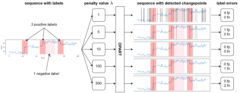
Figure 1: Example of different penalty parameter values result in different sets of changepoints. In this example sequence, there are four labels: three positive labels (regions with only one changepoint each) and one negative label (a region with no changepoint). Different penalty parameter values are experimented with using the OPART algorithm to detect changepoints within this sequence. From the set of changepoints and the predefined labels, there are two types of errors: false positives (fp) – more than one changepoint is detected in a positive label or when at least one changepoint is detected in a negative label, and false negatives (fn) – no changepoint is detected in a positive label. The main question of the study is: To detect changepoint positions from a given the sequence, how can we predict the best penalty parameter value for the changepoint detection algorithms?

Previous methods, such as those employing Bayesian Information Criterion (BIC) (Schwarz, 1978), linear models (Hocking and Srivastava, 2023; Rigaill et al., 2013), ALPIN (Truong et al., 2017) and Maximum Margin Interval Trees (MMIT) (Drouin et al., 2017) have made good attempts to ascertain the optimal $\lambda$ value. However, these methods rely on using linear models or decision trees as learning models may constrain the ability to capture complex patterns.

Given these considerations, this study pursues a unique objective: using deep learning with chosen useful features for penalty parameter prediction. By harnessing the capabilities of deep learning, we aim to uncover complex patterns and relationships within the data, providing a more comprehensive approach to penalty parameter prediction. Our study on three large benchmark supervised labeled datasets shows that the new method consistently outperforms previous ones, demonstrating superior accuracy.

Paper structure

This study is structured into five main sections. Section 1 is the general introduction about the problem of penalty parameter prediction. In Section 2, problem setting and previous methods on penalty parameter prediction is reviewed. Section 3 elaborates on our proposed method, delving into innovative approaches that extend beyond previous methods’ limitations. Section 4 shows the results obtained from applying our proposed method are presented and analyzed comprehensively. Section 5 comprises the discussion and conclusion of the study.

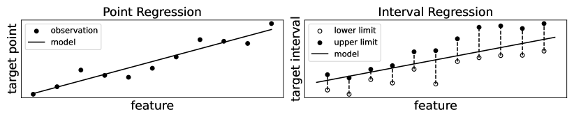
Figure 2: Example of point regression versus interval regression. In the plot on the left, which shows point regression, the model line tries to pass close to all the target points. In the plot on the right, which illustrates censored interval regression, the model line aims to intersect all the intervals.

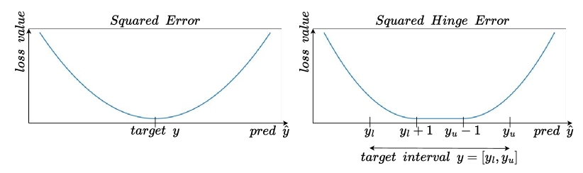
Figure 3: The loss value of two loss functions is determined by comparing the prediction to the target. In the left plot, the squared error loss function yields a value of 0 when the prediction $\hat{y}$ reaches the target point $y$. The right plot illustrates the squared hinge error (this loss function is utilized to predict values falling within a target interval rather than a single target point), where the loss value reaches 0 when the prediction $\hat{y}$ falls within the interval $[y_{l}+1,y_{u}-1]$.

2 Literature Review

2.1 Problem setting

Changepoint detection algorithms take into the sequence $\mathbf{d}$ along with the penalty parameter $\lambda$ as input and then generate the set of detected changepoints. From each sequence $\mathbf{d}$, $M$ distinct labels $\{(s_{i},e_{i},c_{i})\}_{i=1}^{M}$ emerge within the sequence, where $c_{i}$ denotes the expected number of changepoints between points at locations $s_{i}$ and $e_{i}$. Since ALPIN (Truong et al., 2017) requires a predefined expert sequence partition (or equivalently, each positive label having a size of 1, which is a specific special case), it is not suitable for this problem setting. There are two types of label errors: in each label, if the number of detected changepoints greater than $c_{i}$, it’s a false positive; if smaller, it’s a false negative. Finding the optimal set of detected changepoints require considering a range of values for the penalty parameter $\lambda$ (rather than just one specific value) that minimizes the total number of label errors. Consequently, the value of penalty parameter $\lambda$ to be predicted should also fall within an optimal interval, see Figure 2.

This type of problem, where the objective is to find values falling within an interval, is referred to as the interval regression problem. In the interval regression problem, there are four types of intervals: uncensored $(-\infty<y_{l}=y_{u}<\infty)$, censored $(-\infty<y_{l}<y_{u}<\infty)$, left-censored $(-\infty=y_{l}<y_{u}<\infty)$ and right-censored $(-\infty<y_{l}<y_{u}=\infty)$. According to the survey conducted by Wang et al. (2019), the majority of classic statistical parametric models (Tobin, 1958; Kalbfleisch and Prentice, 2002) are learned by assuming the data follow a particular theoretical distribution (commonly used distributions in parametric censored regression models are normal, exponential) and use maximum likelihood to estimate the parameters for these models. This model learning approach differs from the one that will be presented in this section, which involves learning the model by minimizing a specific loss function. While both model learning approaches yield very similar results, minimizing a specific loss function is an simpler approach and being easier to implement.

As a result, squared error, which is commonly used as a loss function in point estimate regression, cannot be employed for this problem. This type of problem requires a different loss function. This loss function, known as squared hinge loss, is defined by Rigaill et al. (2013). The loss function resembles the squared error loss function, except it achieves a loss value of 0 within a target interval, as depicted in Figure 3, unlike the squared error loss function which only achieves 0 loss at a single target point.

Using the ReLU function, the loss value is expressed as follows:

$$l(\hat{y},y)=l(\hat{y},[y_{l},y_{u}])=\big{(}\text{ReLU}(y_{l}-\hat{y}+1)\big{)}^{2}+\big{(}\text{ReLU}(\hat{y}-y_{u}+1)\big{)}^{2}$$

where $\hat{y}$ is the predicted value of penalty parameter $\lambda$ and $y=[y_{l},y_{u}]$, as $y_{l}<y_{u}$ is the optimal interval (lower, upper).

In summary, for each sequence, a vector of sequence features (e.g., length, variance, value range, $\dots$) and the optimal interval of penalty parameter $\lambda$ are obtained. During model training, the vector of sequence features is utilized as input to predict the value of penalty parameter $\lambda$, aiming for it to fall within the optimal interval by minimizing the squared hinge loss function.

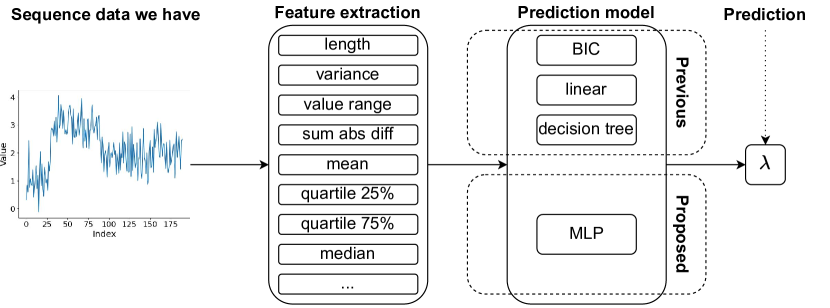
Figure 4: Comparative Model Diagram: Previous Methods versus Our Proposal. From the raw sequence data, various sequence features are extracted such as length, mean, variance, standard deviation, minimum value, maximum value, quartiles, sum of absolute differences, $\dots$ and various transformation functions are applied such as log, absolute, square root, square, or combinations of these. This process yields a large vector of sequence features. However, only the features without missing data or non-infinity values are utilized for learning the penalty parameter value. While previous methods rely on BIC, linear models, or decision trees for penalty parameter prediction, our proposed approach adopts MLPs for enhanced performance.

Notation

Throughout the remainder of this paper, the input of all learning models is referred to as features (extracted from sequence data), while the output is the value of the penalty parameter $\lambda$ to be predicted. So from now, the symbol $\lambda$ refers to the penalty parameter used in the changepoint detection algorithms. The desired predicted value of $\lambda$ falls within an optimal interval, referred to as the target interval. In this paper, labels do not represent the output of the model or the value to be predicted (although in machine learning, labels are sometimes used to denote the value to be predicted). Instead, they denote regions within the sequence characterized by an expected number of changepoints.

2.2 Previous works

Following is a list of previous studies that have worked on predicting the value of $\lambda$, including the Bayes Information Criterion (BIC), linear models and decision trees. Define length as $N_{i}$ and variance as $\sigma_{i}$ for the $i^{th}$ sequence. To maintain consistency with the presentation of the $\lambda$ prediction problem in Rigaill et al. (2013) and Hocking and Srivastava (2023), the following sections will present the prediction problem as predicting $\log\lambda$ instead of $\lambda$.

BIC model

The Bayesian Information Criterion (BIC) proposed by Schwarz (1978) predicts $\log\lambda_{i}=\log\log N_{i}$ for each $i^{th}$ sequence. Notably, this model is unsupervised, it does not involve learning any parameters.

Linear model

This method constructs feature vectors $\mathbf{x}_{i}$ from $i^{th}$ sequence’s features. Prediction of $\log\lambda_{i}=\mathbf{x}_{i}^{T}w+b$ is performed, where parameters $w$ and $b$ are learned using convex optimization with a squared hinge loss. Hocking and Srivastava (2023) utilizes a single feature $\mathbf{x}_{i}=\log\log N_{i}$, while Rigaill et al. (2013) employs a feature vector $\mathbf{x}_{i}=[\log\log N_{i},\log\sigma_{i}]^{T}$. Moreover, Rigaill (2013) employs various statistical features and transformations (square, square root, absolute, log, loglog, $\dots$) to create a large feature vector $\mathbf{x}=[x_{1},x_{2},\dots]$, followed by the application of L1 regularization to address any redundant features.

MMIT

This method, introduced by Drouin et al. (2017), shares a similar concept with regression trees in Breiman et al. (1984). Instead of splitting based on minimizing squared error within regions like in Breiman et al. (1984), MMIT minimizes the hinge loss within each region. The optimal tree architecture, determined by hyperparameters such as maximum depth, minimum sample split and loss margin, is selected through cross-validation on the train set.

They are baseline algorithms will be used as a comparison for the new method. Their limitations and how they are addressed will be discussed in the following section.

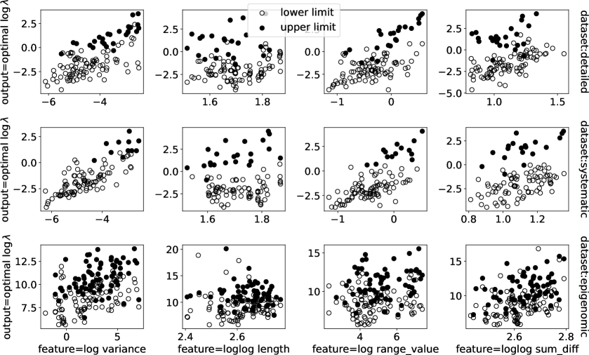
Figure 5: Graphs illustrating the relationship between four features and target intervals. Variance and length are selected because previous studies have incorporated them into the model. Upon examination, we observe that the logarithms of range value, and sum of absolute differences exhibit a discernible increasing monotonic linear relationship with the target interval, indicating their potential as good features.

3 Novelty and contribution

Previous methods are constrained by a limitation: they rely on relatively simple models, such as linear models or decision trees. These models may not fully capture the complexity inherent in the underlying data, potentially leading to suboptimal outcomes.

Our method employs Multi-Layer Perceptrons (MLPs) to predict the value of $\lambda$. Leveraging MLPs for $\lambda$ prediction offers a distinct advantage, as they can extract pertinent hidden features from raw data, mitigating the need for manual feature engineering. Figure 4 provides a comparison summary between our proposed method and previous approaches. In MLPs, employing an excessive number of features is discouraged as the inclusion of irrelevant features can deteriorate the performance. To leverage MLPs effectively, we focus on selecting a subset of key features. In addition to the sequence length and variance utilized in previous methods, we incorporate two additional sequence features: the value range and the sum of absolute differences

• Value range: The value range is defined as the difference between the maximum and minimum values in the sequence. Denoted as $r_{i}$ for $i^{th}$ sequence in Table 1.

• Sum of absolute differences: The sum of absolute differences is calculated as the sum of the absolute differences between two consecutive points in the sequence, denoted as $\sum_{i=1}^{N-1}|d_{i+1}-d_{i}|$, where $\textbf{d}=[d_{1},d_{2},\dots,d_{N}]$ represents the sequence. Denoted as $s_{i}$ for $i^{th}$ sequence in Table 1.

These two features are chosen because intuitively, as the value range or the sum of absolute differences increases, the sequence tends to exhibit more fluctuations and vice versa, suggesting a need to adjust the value of $\lambda$ accordingly.

Furthermore, upon visualizing the relationship between either of these features and the target intervals (representing the range of $\log\lambda$ to minimize training label errors), slightly increasing monotonic relationships are observed. This observation emerged after employing certain feature engineering techniques, see figure 5.

Table 1: List of employed models

(length $N_{i}$ — variance $\sigma_{i}$ — value range $r_{i}$ — sum of absolute difference $s_{i}$) Model Features Model Regularization Citation BIC.1 $\log\log N_{i}$ unsupervised None Schwarz (1978) linear.1 $\log\log N_{i}$ linear None Hocking and Srivastava (2023) Rigaill et al. (2013) Lavielle (2005) linear.2 $\log\log N_{i},\log\sigma_{i}$ linear.4 $\log\log N_{i},\log\sigma_{i},\log r_{i},\log\log s_{i}$, linear.117 117 features linear L1 Rigaill et al. (2013) mmit.1 $N_{i}$ tree max depth min split sample loss margin Drouin et al. (2017) mmit.2 $N_{i},\sigma_{i}$ mmit.4 $N_{i},\sigma_{i},r_{i},s_{i}$, mmit.117 117 features mlp.1 $\log\log N_{i}$ MLP hidden layers number neurons per layer early stopping proposed mlp.2 $\log\log N_{i},\log\sigma_{i}$ mlp.4 $\log\log N_{i},\log\sigma_{i},\log r_{i},\log\log s_{i}$ mlp.117 117 features

4 Experiments

In this section, we will delve into the detailed implementation of our proposed approach aimed at enhancing reproducibility. We begin by processing raw sequence data, with given labels for each sequence, and extracting a set of features along with the target interval using the algorithm outlined by (Rigaill et al., 2013). Subsequently, we implement all baseline methods as well as our proposed method to generate predicted values for $\log\lambda$ (the summary of all employed models is provided in Table 1) Following this, we employ OPART with the predicted values of $\log\lambda$ to obtain the set of changepoints. Finally, leveraging both the set of changepoints and the set of labels, we compute the accuracy rate.

Raw sequence dataset

This study employs three large datasets: two DNA copy number profiles sourced from neuroblastoma tumors (Rigaill et al., 2013) (available at https://github.com/tdhock/neuroblastoma-data), known for their detailed (3730 sequences) and systematic (3418 sequences) data collection. And the last one is a large epigenomic dataset comprising 17 sub-datasets (4913 sequences total) (Hocking et al., 2016) (accessible at https://archive.ics.uci.edu/ml/machine-learning-databases/00439/peak-detection-data.tar.xz).

Evaluation Metrics

The primary evaluation metric utilized is the accuracy rate (percentage) of the test set, which depends on the total number of labels and the total number of label errors. These errors are calculated as the sum of false positives and false negatives across all labels $j$ in the test sets. A false positive occurs when label $j$ exhibits more predicted changepoints than expected for either a positive or negative label. A false negative occurs when the number of predicted changepoints is less than expected in positive labels.

Cross-validation setup

For each dataset, every sequence is assigned a unique identifier, referred to as sequenceID. The dataset is then divided into six folds based on sequenceID. During each iteration, one fold is designated as the test set, while the remaining five folds form the train set. This process is iterated six times, yielding six test accuracy rates. Figure 6 illustrates the median accuracy rate across all six test folds, along with the corresponding 25th and 75th percentile intervals.

Training models

Below are presented the features, target interval, MLP configurations, as well as the loss function and optimizer

Features: Four sets of features are explored:

• 1 feature: sequence length, same as Schwarz (1978) and Hocking and Srivastava (2023)

• 2 features: sequence length and variance, same as Rigaill et al. (2013)

• 117 features: same as Rigaill et al. (2013) and Drouin et al. (2017). There are 117 features selected from a large vector of 365 features, as only those without missing data (values too small for the computer to store) or infinity values are retained.

• 4 features: sequence length, variance, value range, sum of absolute difference (a subset of 117 features to utilize MLPs)

Each feature can be transformed using either the $\log(\cdot)$ or $\log\log(\cdot)$ function (see Table 1) to ensure compatibility and enable straightforward comparisons with previous methods (BIC and linear models).

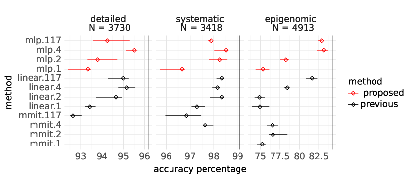
Figure 6: Median test accuracy and interquartile range (25% to 75%) across 6 folds for each method. To enhance clarity in the comparison visualization, method BIC and some small accuracies have been omitted (in the dataset detailed, methods mmit.1, mmit.2, and mmit.4 are excluded. In the dataset systematic, methods mmit.1 and mmit.2 are omitted. In the dataset epigenomic, method mmit.117 is not included). Across all three datasets, mlp.4 exhibits superior accuracy compared to all baseline methods, boasting higher median accuracy as well as improved accuracy interquartile.

Target intervals: Every sequence within each dataset comes with its own set of labels, indicating the expected number of changepoints within specific regions. For each sequence, the target interval is the range of $\lambda$ value that minimizes the number of label errors (for each sequence with its set of detected changepoints, the minimum number of label errors is 0, and the maximum number of label errors is equal to the number of labels assigned to the sequence), which can be achieved by employing the algorithm described by Rigaill et al. (2013).

Model Configurations Implementation: All baseline models (BIC, linear and decision tree) and MLPs with four different sets of features were employed (13 of them). To implement each MLP model, a two-fold cross-validation was employed on the train set to determine the optimal number of hidden layers and the number of neurons per hidden layer. This selection was based on achieving the highest accuracy rate on the corresponding validation set. Different MLP configurations were validated, including models with 1 to 4 hidden layers and all hidden layer of one model can have sizes of 2, 4, 8, 16, 32, 64, 128, 256 or 512 neurons.

Number of iterations with Early Stopping: The early stopping technique, recommended by Prechelt (2012), controls the number of iterations. It uses the "patience" parameter to decide when to stop learning. During neural network training, setting a large maximum number of iterations and specifying the value for patience parameter allows for monitoring the training process. If the loss value from the train set does not decrease after the specified number of patience iterations, the training process is halted. This technique helps prevent overfitting. In our study, we set the maximum number of iterations to 12000 and patience parameter value to 20 iterations.

Random seed setting: Due to the use of random seeds, each time we initialize the parameters in an MLP model, we obtain a different set of initial values. Consequently, this leads to variability in the trained models. However, after testing with numerous random seeds, we observed that the outcomes closely resemble those depicted in Figure 6.

Loss function and optimizer: The Adam optimizer is employed to minimize the squared hinge loss function (linear models and MLPs).

Table 2: Chosen MLP configuration count across 6 folds for each dataset

layers	neurons	detailed				systematic				epigenomic				total
		1	2	4	117	1	2	4	117	1	2	4	117
1	$\leq 64$		1		1	1	1	2	1		2		2	11
	$>64$					2		1	1					4
2	$\leq 64$	1	2	4	1				2	2	1	5	4	22
	$>64$				2			1						3
3	$\leq 64$	5	2			1	1	1		4	3			17
	$>64$						2							2
4	$\leq 64$		1	1	2	2	1		1			1		9
	$>64$			1			1	1	1					4

For each model MLP from each dataset, 6 folds are tested, resulting in the selection of 6 MLP configurations. Dataset detailed has 3,730 sequences, systematic has 3,418, and epigenomic has 4,913. Observing the trend in the table, it’s evident that the preference leans towards MLPs with 2 or 3 hidden layers and the number of neurons is less than 64. Specifically, out of the 72 chosen architectures, 15 have 1 hidden layer, 25 have 2 hidden layers, 19 have 3 hidden layers, and 13 have 4 hidden layers.

5 Discussion and conclusion

Discussion:

Effect of Feature Selection: The experiments reveal that accuracy improves when a larger set of features (except in the case of 117 features) is integrated, compared to using fewer features, across linear, decision tree, or MLP models. Perhaps the reason lies in the better quality of the larger feature set. If we closely examine the feature sequence length in Figure 5, the relationship between sequence length and the target interval of $\lambda$ is not entirely clear. This lack of clarity could explain why models relying solely on this feature exhibit lower accuracy compared to others. Remarkably, nonlinear models such as decision trees or MLPs exhibit lower accuracy when employing 117 features compared to when using only 4 features. So selecting only 4 features proves highly beneficial, enhancing model accuracy (both linear models and MLPs) while also potentially reducing training time for the models. This divergence can be attributed to the inherent challenge faced by MLPs in effectively eliminating unnecessary features.

Using MLPs effect: employing MLPs with appropriate configuration (see Figure 7 and Table 2) yields a enhancement in accuracy when contrasted with linear models. In the case of the same feature set, it’s not guaranteed that MLPs will consistently outperform linear models. For instance, in the dataset detailed, the linear model with two features perform better than the MLP. Similarly, in the dataset systematic, the linear model with one feature has the better performance than the MLP.

Comparison of MMIT and Linear Model Accuracy: In many cases where the number of features remains constant, MMIT does not outperform linear models. This is often due to observable linear relationships between features and target intervals (see Figure 5). Intuitively, linear models are perceived as superior to decision trees under such circumstances.

Conclusion: MLP models with chosen four features generally achieve higher accuracy in changepoint detection compared to linear models and decision trees. However, it’s important to note that the training process for MLPs is significantly more time-consuming than that for linear models.

Limitations of this study: There are several considerable limitations from this study below

May not be applicable to other sequence datasets: Intuitively, features such as variance, value range, and sum of absolute difference play a role in predicting this penalty problem for these particular benchmark datasets. However, these features may not be relevant in other types of sequence datasets.

May overlook some other useful features: By focusing on a limited number of features and their relationship with target intervals, we may overlook additional useful features and potential interactions between features.

Challenges in Selecting the Optimal MLP Configuration The process of identifying the most suitable MLP configuration is inherently time-consuming. It entails evaluating a plethora of configurations, each comprising different combinations of hidden layers and neurons. Our task entails validating 36 distinct MLP models for each pair of train and test sets (we considered variations in the number of hidden layers, ranging from 1 to 4, and the number of neurons per layer, which can be 2, 4, 8, 16, 32, 64, 128, 256, or 512). This exhaustive exploration represents a significant computational challenge. Furthermore, we did not delve into exploring architectures with varying neuron counts across layers within a single model.

Future Work: Various neural network architectures can be explored. Beyond MLPs, one might investigate the performance of other architectures tailored to the specific characteristics of the data. In some cases, these alternative network structures may yield superior results compared to MLPs or linear models. About feature selection, instead of manual feature extraction, it could be worthwhile to explore Recurrent Neural Networks (RNNs) (Hopfield, 1982) for directly extracting features from raw sequences. Variants like Gated Recurrent Units (GRUs) (Cho et al., 2014) or Long Short-Term Memory networks (LSTMs) (Hochreiter and Schmidhuber, 1997) could be examined for this task. Moreover, as feature transformations like logarithmic scaling were employed, it’s worth exploring alternative approaches to feature engineering.

Reproducible Research Material: For those interested in replicating our study, all the code and associated materials are available at this link:
github.com/lamtung16/ML_ChangepointDetection. This commitment to reproducibility ensures transparency and allows others to validate and build upon our findings.

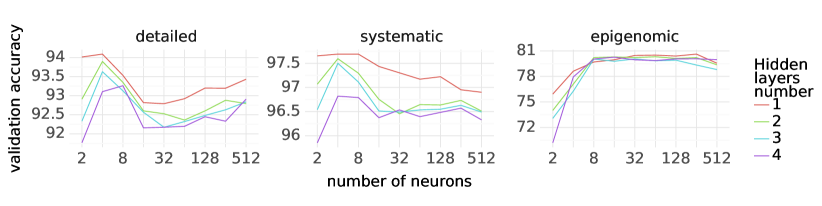
Figure 7: MLP configurations’ average validation accuracies, regardless of number of features. For datasets detailed and systematic, it’s generally preferable to have fewer hidden layers, typically around 4 to 8 neurons per layer suffice. In dataset epigenomics, where accuracy remains relatively consistent across various numbers of hidden layers, optimal accuracy tends to be achieved with a neuron count ranging from 8 to 256.

References

- Breiman et al. [1984] L. Breiman, J. H. Friedman, R. A. Olshen, and C. Stone. Classification and regression trees (cart). Biometrics, 40(3):358, 1984.
- Cho et al. [2014] K. Cho, B. van Merriënboer, C. Gulcehre, D. Bahdanau, F. Bougares, H. Schwenk, and Y. Bengio. Learning phrase representations using RNN encoder–decoder for statistical machine translation. In A. Moschitti, B. Pang, and W. Daelemans, editors, Proceedings of the 2014 Conference on Empirical Methods in Natural Language Processing (EMNLP), pages 1724–1734, Doha, Qatar, Oct. 2014. Association for Computational Linguistics. doi: 10.3115/v1/D14-1179. URL https://aclanthology.org/D14-1179.
- Drouin et al. [2017] A. Drouin, T. D. Hocking, and F. Laviolette. Maximum margin interval trees. In Proceedings of the 31st International Conference on Neural Information Processing Systems, NIPS’17, page 4954–4963, Red Hook, NY, USA, 2017. Curran Associates Inc. ISBN 9781510860964.
- Hochreiter and Schmidhuber [1997] S. Hochreiter and J. Schmidhuber. Long short-term memory. Neural Comput., 9(8):1735–1780, nov 1997. ISSN 0899-7667. doi: 10.1162/neco.1997.9.8.1735. URL https://doi.org/10.1162/neco.1997.9.8.1735.
- Hocking and Srivastava [2023] T. D. Hocking and A. Srivastava. Labeled optimal partitioning. Computational Statistics, 38(1):461–480, 2023. ISSN 0943-4062. doi: 10.1007/s00180-022-01238-z.
- Hocking et al. [2014] T. D. Hocking, V. Boeva, G. Rigaill, G. Schleiermacher, I. Janoueix-Lerosey, O. Delattre, W. Richer, F. Bourdeaut, M. Suguro, M. Seto, et al. Seganndb: interactive web-based genomic segmentation. Bioinformatics, 30(11):1539–1546, 2014.
- Hocking et al. [2016] T. D. Hocking, P. Goerner-Potvin, A. Morin, X. Shao, T. Pastinen, and G. Bourque. Optimizing ChIP-seq peak detectors using visual labels and supervised machine learning. Bioinformatics, 33(4):491–499, 11 2016. ISSN 1367-4803. doi: 10.1093/bioinformatics/btw672. URL https://doi.org/10.1093/bioinformatics/btw672.
- Hopfield [1982] J. J. Hopfield. Neural networks and physical systems with emergent collective computational abilities. Proceedings of the National Academy of Sciences, 79(8):2554–2558, 1982. doi: 10.1073/pnas.79.8.2554. URL https://www.pnas.org/doi/abs/10.1073/pnas.79.8.2554.
- Jackson et al. [2005] B. Jackson, J. D. Scargle, D. Barnes, S. Arabhi, A. Alt, P. Gioumousis, E. Gwin, P. Sangtrakulcharoen, L. Tan, and T. T. Tsai. An algorithm for optimal partitioning of data on an interval. IEEE Signal Processing Letters, 12(2):105–108, 2005.
- Kalbfleisch and Prentice [2002] J. D. Kalbfleisch and R. L. Prentice. The Statistical Analysis of Failure Time Data. Wiley, Aug. 2002. ISBN 9781118032985. doi: 10.1002/9781118032985. URL http://dx.doi.org/10.1002/9781118032985.
- Lattanzi and Leonelli [2021] C. Lattanzi and M. Leonelli. A change-point approach for the identification of financial extreme regimes. Brazilian Journal of Probability and Statistics, 35(4), Nov. 2021. ISSN 0103-0752. doi: 10.1214/21-bjps509. URL http://dx.doi.org/10.1214/21-BJPS509.
- Lavielle [2005] M. Lavielle. Using penalized contrasts for the change-point problem. Signal Processing, 85(8):1501–1510, 2005. ISSN 0165-1684. doi: https://doi.org/10.1016/j.sigpro.2005.01.012. URL https://www.sciencedirect.com/science/article/pii/S0165168405000381.
- Muggeo and Adelfio [2010] V. M. R. Muggeo and G. Adelfio. Efficient change point detection for genomic sequences of continuous measurements. Bioinformatics, 27(2):161–166, 11 2010. ISSN 1367-4803. doi: 10.1093/bioinformatics/btq647. URL https://doi.org/10.1093/bioinformatics/btq647.
- Prechelt [2012] L. Prechelt. Early Stopping — But When?, page 53–67. Springer Berlin Heidelberg, 2012. ISBN 9783642352898. doi: 10.1007/978-3-642-35289-8_5. URL http://dx.doi.org/10.1007/978-3-642-35289-8_5.
- Reeves et al. [2007] J. Reeves, J. Chen, X. L. Wang, R. Lund, and Q. Q. Lu. A review and comparison of changepoint detection techniques for climate data. Journal of Applied Meteorology and Climatology, 46(6):900–915, June 2007. ISSN 1558-8424. doi: 10.1175/jam2493.1. URL http://dx.doi.org/10.1175/JAM2493.1.
- Rigaill et al. [2013] G. Rigaill, T. D. Hocking, F. Bach, and J.-P. Vert. Learning Sparse Penalties for Change-Point Detection using Max Margin Interval Regression, June 2013. URL https://inria.hal.science/hal-00824075.
- Schwarz [1978] G. Schwarz. Estimating the Dimension of a Model. The Annals of Statistics, 6(2):461 – 464, 1978. doi: 10.1214/aos/1176344136. URL https://doi.org/10.1214/aos/1176344136.
- Tartakovsky et al. [2013] A. G. Tartakovsky, A. S. Polunchenko, and G. Sokolov. Efficient computer network anomaly detection by changepoint detection methods. IEEE Journal of Selected Topics in Signal Processing, 7(1):4–11, 2013. doi: 10.1109/JSTSP.2012.2233713.
- Tobin [1958] J. Tobin. Estimation of relationships for limited dependent variables. Econometrica, 26(1):24, Jan. 1958. ISSN 0012-9682. doi: 10.2307/1907382. URL http://dx.doi.org/10.2307/1907382.
- Truong et al. [2017] C. Truong, L. Gudre, and N. Vayatis. Penalty learning for changepoint detection. In 2017 25th European Signal Processing Conference (EUSIPCO), pages 1569–1573, 2017. doi: 10.23919/EUSIPCO.2017.8081473.
- Wang et al. [2019] P. Wang, Y. Li, and C. K. Reddy. Machine learning for survival analysis: A survey. ACM Comput. Surv., 51(6), feb 2019. ISSN 0360-0300. doi: 10.1145/3214306. URL https://doi.org/10.1145/3214306.