arrow/.style=thick, shorten >=5pt,shorten <=5pt,->, photon/.style=decorate, decoration=snake, style=thick, electron/.style = decoration= markings, mark=at position 0.5 with \arrow[xshift=1mm]Stealth[width=1mm,length=2mm], postaction=decorate, style=thick, electronNoMu/.style = decoration= markings, mark=at position 0.5 with \arrow[xshift=1mm]Stealth[width=1mm,length=2mm], postaction=decorate, style = thick, dashed
Exceptional Luttinger Liquids from sublattice dependent interaction
Abstract
We demonstrate how Exceptional Points (EPs) naturally occur in the Luttinger Liquid (LL) theory describing the low-energy excitations of a microscopic lattice model with sublattice dependent electron-electron interaction. Upon bosonization, this sublattice dependence directly translates to a non-standard sine-Gordon-type term responsible for the non-Hermitian matrix structure of the single-particle Green Function (GF). As the structure in the lifetime of excitations does not commute with the underlying free Bloch Hamiltonian, non-Hermitian topological properties of the single-particle GF emerge – despite our Hermitian model Hamiltonian. Both finite temperature and a non-trivial Luttinger parameter are required for the formation of EPs, and their topological stability in one spatial dimension is guaranteed by the chiral symmetry of our model. In the presence of the aforementioned sine-Gordon-term, we resort to leading order Perturbation Theory (PT) to compute the single-particle GF. All qualitative findings derived within LL theory are corroborated by comparison to both numerical simulations within the conserving second Born approximation, and, for weak interactions and high temperatures, by fermionic plain PT. In certain parameter regimes, quantitative agreement can be reached by a suitable parameter choice in the effective bosonized model.
I Introduction
Luttinger Liquid (LL) 111Tomonaga-Luttinger Liquids [6, 27, 30, 63, 64, 38] (or even Landau-Luttinger Liquids [4]), originate from the Tomonaga-Luttinger model [84, 85, 5, 23, 69, 86, 9, 10, 13, 29] and are often simply referred to as Luttinger Liquids [2, 69, 8, 9, 13, 29] in analogy to Landau’s Fermi Liquid [87, 14, 88, 4, 5, 89, 23, 69, 8, 16]. theory provides an important toolbox for describing the low energy properties of one-dimensional (1D) correlated electrons as an effective bosonic field theory [2, 3, 4, 5, 6, 7, 8, 9, 10, 11, 12, 13]. In higher spatial dimensions, Landau’s Fermi Liquid theory tells us that the lifetime of quasi-particle excitations generically diverges with temperature as at the Fermi surface [14, 15, 16], thus justifying an independent particle approximation. By contrast, in 1D the lifetime [17, 18] of single-particle type electronic excitations defies a free effective description, which may be remedied by bosonization in the framework of LL theory in a wide range of settings [19, 20, 21, 22, 23, 24, 25, 26, 27, 28, 29, 30, 31, 32, 33, 34, 35, 36, 37, 38].
Realistic experimental circumstances to some extent deviate from the ideal zero temperature fixed point, hence putting finite lifetime effects back on the table in any of the aforementioned scenarios. When scattering rates acquire a non-trivial matrix structure in some orbital or spin degree of freedom, imaginary parts of excitation spectra may be promoted to intriguing non-Hermitian (NH) topological properties [39, 40, 41, 42, 43, 44, 45, 46, 47, 48, 49] such as exceptional degeneracies [50, 51, 52, 53, 54, 55, 56, 57, 58].
In the context of LLs, despite the peculiar role of lifetime effects in 1D, NH physics has thus far only been considered for -symmetric Hamiltonians [59, 60, 61], or by phenomenologically adding external dissipation terms [62, 63, 64]. Both of these cases have in common that the initial model is already explicitly NH.
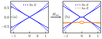
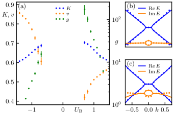
Here, we demonstrate how EPs naturally emerge in LL Theory by bosonizing and studying a Hermitian microscopic one-dimensional lattice model of fermions with sublattice-dependent interactions. Upon linearizing the dispersion relation of an extended critical Su–Schrieffer–Heeger (SSH) model [65, 66] (see Fig. 1a), bosonization leads to a novel sine-Gordon-type interaction term of the form , where is the lattice spacing. We compute the single-particle Green Function (GF) at finite temperature by treating this term in Matsubara Perturbation Theory (PT) to leading order. Note that in our construction it is necessary to keep the lattice spacing finite to obtain rigorous results. This gives rise to an intricate residue structure, and we handle the relating technical challenges by breaking the problem down into manageable parts.
Analytic continuation to real frequencies and inference of an effective NH Hamiltonian from the GF then yields quasi-particle spectra that feature EPs (see Fig. 1b) in an extended parameter range. We demonstrate these properties by numerically implementing our perturbative solution along with an analytical continuity argument exploiting the chiral symmetry (CS) of the model. We quantitatively analyze how the four important parameters, inverse temperature , Luttinger parameter , renormalized Fermi velocity and effective coupling , continuously impact the EPs. To corroborate our findings, we also provide comparisons to complementary methods based on plain fermionic PT, as well as a fully numerical approach via Conserving Second Born Approximation (CSBA).
Outline.
In Section II, we introduce and bosonize our model. The single-particle GF is perturbatively computed in Section III. The NH topology of the corresponding effective Hamiltonian is subsequently discussed in Section IV, where we also provide quantitative comparisons to results from fermionic PT and microscopic numerics via CSBA. In Section V, we conclude our results and provide an outlook.
II Model and Low-Energy Theory
In Section II.1, we introduce the microscopic lattice model which we subsequently bosonize in Section II.2.
II.1 Fermionic lattice model
We consider an extended SSH model given by [56]
| ((1)) |
where is the number of sites and are real-valued hopping parameters, and we focus on the gapless regime . The two-component annihilation operators act on site , and the indices refer to the respective sublattice. Note that , i.e. we assume periodic boundary conditions. We introduce Fourier modes via , where is the lattice spacing and the sum runs over momenta with for even . Linearizing the dispersion around the Fermi energy yields
where is the Fermi velocity. To model interactions between the particles, we include a sublattice-dependent density-density term given by [56, 45, 49]
| ((2)) |
Here, is the density operator, denotes nearest neighbors and . We assume half-filling, thus due to translational invariance (one particle per unit cell). The free Hamiltonian also admits sublattice symmetry, , and therefore as in Ref. [56].
Note that the interaction strengths and on the sublattices are allowed to be different, which is a key requirement for EPs, as it introduces sublattice staggering in the scattering rates. Furthermore, one requirement for EPs is a non-trivial matrix structure of the self-energy , i.e. [56, 51, 49]. For this should be satisfied, because the interaction term facilitates a -contribution, while corresponds to .
Fig. 1 illustrates the dispersion relation with and without interactions. In concrete examples, such as the above, we always use the parameter values and .
II.2 Bosonization
Before applying bosonization, we first diagonalize by introducing left- and right-movers with , which gives 222This is essentially the kinetic part of the Tomonaga-Luttinger model [90, 10]. (we identify and , as well as and )
With and the interaction can be split into
Using the replacement [68], we write in the spirit of a continuum limit. The bosonization identity reads
| ((3)) |
where denotes normal-ordering with respect to the bosonic operators [6, sec. 10.A]. The bosonic fields are given by with
and . Ideally, the UV regulator should be taken to zero, but one may argue that it can also mimic a finite bandwidth [6, sec. 5]. However, this leads to a subtle issue with fundamental properties of the GFs that we discuss in Section III.
For the dispersion is decreasing – thus we have to count the momenta in the opposite way – which amounts to the replacement [6, sec. 10.A]. It is more convenient to adjust the relations impacted by undoing this change via , which leads to additional factors of (e.g. the exponent of ).
In the thermodynamic limit, the Klein factors become Hermitian [69, p. 25] and we may neglect the additional phase factor in Eq. (3). The density operator and standard commutation relations are then given by
Our model takes the form , where (see Appendix A for details)
corresponds to an interacting LL with Luttinger parameter , renormalized Fermi velocity and the fields . The remaining perturbations read
and we refer to as the Exceptional Luttinger Liquid (ELL). Note that itself is still Hermitian and that it is not straightforward to take either limit , as this would give a trivial and eliminate due to its integrand becoming a total derivative.
III Perturbative Approach
In this section, we are interested in the single-particle Matsubara Green Function that in fermionic and bosonic language is given by (imaginary time )
Due to the complex (non-bilinear) nature of the model, an exact evaluation of the expectation value is infeasible, and we instead resort to a perturbative approach. We start by computing the free GF in Section III.1, before discussing the first order corrections in Section III.2.
III.1 Zeroth order
We intentionally write in a form that is not normal-ordered, because one can evaluate the expectation value of an arbitrary product of vertex operators,
Here, we introduce with the dimensionless variables for each space-time point . Furthermore, we write and assume the neutrality conditions and ; otherwise the right hand side is zero [70, sec. 3; 12, app. C]. The function is given by (see Appendix B)
where . Interestingly, although the condition for the asymptotic equality is not always satisfied, the approximation of appears to be the physically correct result. To see why, consider the single-particle Matsubara GF for ,
| ((4)) |
where . This result is consistent with the generic anti-periodicity of fermionic Matsubara GFs, but only within the asymptotic limit , i.e. for the approximate form of . Nevertheless, this matches the result stated in literature, e.g. [9, sec. IV.C; 17, sec. III.A; 18; 71, sec. 6.8.4].
The Fourier Transform (FT) of (see Appendix B.2 for details) leads to
where for are the fermionic Matsubara frequencies and the functions are defined in Appendix B. As a side note, the FT of to via a straightforward application of the residue theorem yields the lifetime in accordance with [18].
III.2 Leading corrections
For now, we ignore and focus on the perturbation . Then the first order correction is
where , corresponds to but with shifted spatial coordinate , and is implied. The neutrality violating factor drops out due to , and the neutrality condition requires and . The time-ordering splits the integration over , but one can show that it is possible to recombine the two parts by carefully treating sign factors. Thus we find
with and . The FT can be performed via the Convolution Theorem (CT) and leads to , where
with defined in Appendix B. Performing the analytic continuation is now straightforward and yields the retarded GF to first order in . Note that we identify the ratio
| ((5)) |
as the “small quantity” of the perturbation series, and coincides with several breakdowns of the theory, e.g. positive imaginary energies and unphysical divergences.
We can justify disregarding the perturbation for the calculation of the GF via a Renormalization Group (RG) argument. For this purpose, we use a standard perturbative momentum-shell RG [3, 72, 73, 71]. Consistent with power counting, the tree-level flow equations are
where at RG-time we have and . Thus, is indeed irrelevant for (which is typically satisfied, see Section IV.3). In Appendix C, we also derive the one-loop corrections for an arbitrary cut-off function.
IV Exceptional Points
Using the single-particle GF, the effective Hamiltonian can be defined as , or, in terms of the self-energy, as [52, 55, 74]. In Section IV.1, we discuss our results by analysing the quasi-particle spectrum of with a focus on the occurrence and stability of EPs. We discuss the quantitative dependence of the characteristic parameters of the EPs in Section IV.2 and compare to CSBA as well as fermionic plain PT in Section IV.3.
IV.1 Symmetries of the effective Hamiltonian
In the following, quantities are always assumed to be in the AB-basis, i.e. indices correspond to a sublattice. Whenever an object is instead in the basis of left- and right-movers, we denote it with a subscript.
Our result for the single-particle GF takes the form
where and . Writing , we have . Here, is the vector of Pauli matrices, , and by construction () is symmetric (anti-symmetric) in .
Our model admits chiral symmetry with the transformation matrix in the AB-basis. The important consequence of this symmetry is the relation [56] (see Appendix E.3 for a derivation)
for the effective Hamiltonian defined via the single-particle GF . Due to the -matrix structure we can write (arguments and are omitted), where and with . The conditions for an EP then become [54]
| ((6)) |
and in one dimension stable EPs generically require an additional symmetry to reduce the codimension of these equations: In our case, the chiral symmetry trivializes at the Fermi energy [43].
Let us now explicitly compute the coefficients and demonstrate the occurrence of EP. With from Section II.2,
where . Omitting the frequency argument, the functions and d are then given by 333Note that we have the general result for non-singular matrices.
Since , this means that and are symmetric in , while is anti-symmetric. Due to , we have . Similarly , and lead to , and thus the remaining condition for an EP simplifies to . By construction , so must be increasing on some interval . Fixing such a , we then have for sufficiently small , and consequently an EP must exist by virtue of the intermediate value theorem (note that because the imaginary part of the -integrand is symmetric).
IV.2 EPs and parameter dependence
The complicated structure of the formal solution makes quantitative comparison to fermionic PT and CSBA difficult. We therefore proceed to numerically explicate our formal solution for the GF.
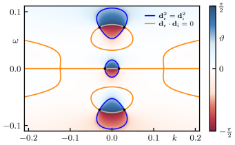
The energies are and is the phase of the energy gap; Fig. 2 illustrates our ELL result for a specific choice of parameters. Note that qualitatively this is remarkably similar to the brute force numerical results in Ref. [56]: Our result shares all the symmetries and features, such as the three arcs protruding from the horizontal line, and the additional pair of EPs at finite . The main visual difference is that, in the CSBA result, the three lobes of are connected into one contour. However, this is merely a quantitative problem, and one should keep in mind that the temperatures are very different.
Fig. 3 illustrates the dependence of the EP on the four parameters , , and .
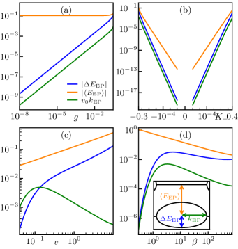
Fermi liquid theory breaks down in one dimension, because the lifetime asymptotically scales as [18], and thus does not diverge fast enough for well-defined quasi-particles. Yet, it is still natural to expect any imaginary parts at to vanish in the zero temperature limit. Panel (d) demonstrates this, as the EPs shrink as , albeit slowly ( for , slightly modified for finite ).
IV.3 Comparison to other methods
In this section, we compare our first order ELL PT to fermionic second order plain PT (see Appendix D), as well as to the numerics on the full lattice model within CSBA along the lines of Ref. [56]. This comparison is challenging, because the regions in which the three methods are valid are almost disjoint: The ELL PT is limited to comparatively low temperatures , while the range of validity is for the fermionic PT. CSBA requires interactions strengths to make interaction effects visible at the feasible system sizes, which is roughly the upper bound for the fermionic PT.
Using the explicit formulas for , and from Section II.2 does not yield quantitative agreement, and we instead use them as fit parameters to demonstrate that the ELL PT can in principle reproduce the results from the other methods. The hope is that it might then be possible to predict these values via a Renormalization Group analysis; we briefly discuss this in Appendix C. The results of this fit to the fermionic PT for and CSBA for are shown in Fig. 4 and Fig. 5 respectively. We once again fix , but smaller merely lead to a constant shift of the values for (since , smaller give smaller ). This is because the EPs only depend on the ratio between and , and a change in can thus always be compensated by a change in .
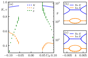
Note that qualitatively, the figures are almost identical. Let us start the discussion starting from the right of panel (a), i.e. . Here, both the fermionic PT and CSBA predicts a small real-valued gap, which is not contained in the ELL result (this is a consequence of the linearization eliminating the -part). Since there are no EPs, and is determined by the imaginary part of the energy, while roughly corresponds to the slope of the linear section (this is also the case for ).
As is decreased, the coupling increases – but contrary to the microscopic prediction, the increase is exponential rather than linear. Furthermore, while at least qualitatively a decrease in is to be expected, the value of is much further from the simple . Unsurprisingly, the exponential growth of rapidly increases , and at around ( or ) we can no longer obtain a reasonable fit using our first order ELL PT. Intuitively, approaching is infeasible even if truncating the perturbation series at a higher order. This is because the “bubble” constituting the imaginary energy gap has to touch the origin at . But, in the language of the ELL this scenario is highly unstable, as an arbitrarily small increase in would then immediately lead to a positive imaginary energy. Another hint that this barrier may be insurmountable is the qualitative change in the behavior for : Evidently, the dependence of is once again exponential, but despite the increase in the coupling actually goes down. Similarly, the decrease in would naively lead to an increase of towards unity, while we observe the opposite. Finally, is much larger than for (which also compensates for the significantly smaller coupling, see Fig. 3c).
At least partially, the quantitative problems are presumably due to the comparatively high temperature of . Using the linearized instead of the exact dispersion in the fermionic PT also leads to strong deviations, which suggests the excitation of degrees of freedom beyond the momenta where the linearization provides a good approximation. Consequently, there is every reason to assume that the LL approach suffers from this as well, and that the accuracy significantly improves for larger (e.g. as chosen for Fig. 2).
V Concluding discussion
By bosonizing and perturbatively solving a microscopic lattice model with sublattice dependent interaction in the low energy limit, we have demonstrated how exceptional points naturally emerge in Luttinger liquid theory. The essential new component is the sine-Gordon-type perturbation , which at finite temperature and for a non-trivial Luttinger parameter leads to the formation of Exceptional Points. Qualitatively, our analytic results match predictions from numerical CSBA data for the microscopic model along the lines of [56] as well as plain fermionic Perturbation Theory. The structural similarity of our Fig. 2 to Fig. 2 in [56] is particularly striking. Quantitative agreement in our present analysis requires fitting parameters of the effective bosonized model to the numerical data. It might be possible to even predict these parameter values via RG, where non-perturbative schemes might be necessary since we work quite far from the zero temperature fixed point.
While this issue is not specific to our model, we find it unsatisfactory that, for , there is a residual dependence on the UV cut-off in the final result. Although a finite value of can be argued via RG (or for a nearest-neighbor interaction [12, sec. 2.2.2]), the analytic inconsistency with the fundamental periodicity of Matsubara GFs remains. On a similar note, we cannot quite take a proper continuum limit for the bosonized Hamiltonian, because setting eliminates the all-important perturbation . Interestingly, this problem cannot easily be solved by an expansion in the lattice spacing, as intermediate results are non-perturbative in due to the residue structure in certain integrals. Thus, removing the mild non-locality induced by while retaining the EPs requires additional insight.
Beyond our present study showing that Luttinger Liquid theory is capable of describing EPs, it will be interesting to see which other NH phenomena, such as the NH Skin Effect or the anomalous spectral sensitivity of NH systems can be investigated using the Luttinger Liquid framework.
Acknowledgements.
We acknowledge financial support from the German Research Foundation (DFG) through the Collaborative Research Centre (SFB 1143, project ID 247310070) and the Cluster of Excellence ct.qmat (EXC 2147, project ID 390858490). Our numerical calculations were performed on resources at the TU Dresden Center for Information Services and High Performance Computing (ZIH).Appendix A ELL bosonization details
In this section, we give some additional details of the bosonization procedure for the ELL left out in Section II.2.
Recall that , where
Since , we may also drop the regularization for the corresponding terms. Eq. (3) then leads to
Normal-ordering the bilinear only amounts to an irrelevant additive constant, and introducing new fields via yields
Here, as well as in the following, the asymptotic limit is always implied. By using the commutation relation
we can normal-order the product of vertex operators, , by rewriting it as
To normal-order , first note that for leads to This commutator can then be used to rewrite as
The similar expression for is already normal-ordered and, since we sum on , this leads to
Interestingly, the product in therefore already is normal-ordered and thus far the full Hamiltonian is , where
At first glance taking the continuum limit seems to be an easy task: keep fixed while . There are, however, several issues with this procedure. The asymptotic expansion of boils down to
Summing on gives , which would exactly cancel the term from the continuum limit of if not for the modified denominator .
Even subtleties involving aside, the continuum limit for is much more troublesome. The integrand turns into the total derivative and therefore the contribution vanishes. The result would then no longer depend on the difference between the interaction strengths, but we already know this to be a crucial ingredient from the numerical analysis in [56]. For now, we tentatively accept that this limit is not straight-forward and simply keep the exact expression.
Absorbing the density-density terms from and into by modifying the coefficients then leads to the ELL presented in Section II.2.
Appendix B Green Function of the ELL
In Section B.1, we give a brief overview of the technical results that were skipped during the evaluation of the GF of the ELL in Section III. In Section B.2, we then derive these results in more detail.
B.1 Overview of the results
Computing correlators can then be done directly on the operator level and we define . Dropping the label for notational convenience, this evaluates to
where . Expanding the hyperbolic cosine and the Bose function yields 444 for
In the thermodynamic limit, this result is plagued by an infrared (IR) divergence, so we instead consider the regularized expression , which gives
where ( in Section III). Utilizing the product representation of the Gamma function one can readily verify that , which yields the expression stated in Section III.
For the calculation of the single-particle GF of the ELL, we define the set of special functions
| ((7)) |
where . One can show that at (for even) and at (for odd), these functions admit the integral representation (see Appendix B.2)
where and . Thus, corresponds to the FT of the free GF. At first order Perturbation Theory, we encounter the integral
with . The solution is given by (see Appendix B.2)
where, with and ,
B.2 Detailed derivations
Derivation of .
In the following, one should think of the function as being defined by the integral representation; the goal is to show that this reduces to Eq. (7). It is sufficient to solve the integral for a single , because one can then recursively obtain the general result. To illustrate the idea behind this recursion, consider to be odd and note that equals
Of course a similar relation holds for even, as well as different frequency arguments. In the spirit of an inductive argument, we assume that Eq. (7) holds for and insert it to get
where . Using the recursive property of the Gamma function, , these can be rewritten as
Plugging this into our previous result yields
which corresponds to Eq. (7). Similarly, one can verify that the relation also holds for , and of course the case of even is analogous too.
Now all that is left to do is to solve the integral for some . While a direct calculation for might be doable due to the additional symmetry of the integral, there exists a more elegant approach for the case of . Since this is equivalent to the FT of Eq. (4), it must correspond to the retarded GF of an interacting LL (whose FT turns out to be much easier to compute). Similar to the calculation for the Matsubara GF, we define and find that yields
The retarded GF also contains a similar term from the anti-commutator, which we can obtain from the above by substituting . This replacement has a rather subtle consequence that originates from the fractional exponentiation of real numbers: In our case, this leads to the phase factors
and hence a global minus sign if . Combining the two terms is thus equivalent to multiplication by an additional factor of the form
for . The latter is a valid assumption, because the retarded GF contains a factor of , and thus evaluates to (only is non-zero)
where . The two-dimensional FT can also be rewritten in terms of the light-cone variables , i.e. becomes
This is valid, because the Heaviside function limits the integration region to , which corresponds to . With , inserting our expression for the retarded GF and using finally yields
The idea at this point is to realize that, if the analytic continuation is possible for the result of the FT of Eq. (4), it must be identical to the above. More explicitly, rescaling the integration variables gives
This is consistent with our result for the retarded GF if, and only if,
which is clearly equivalent to Eq. (7) for .
Derivation of .
The integral representation only holds , where . Since we already know the FT without the extra cotangent, it would be natural to split off this factor via the CT. We choose to split off an additional cosecant factor as well, because this later makes the convolution in momentum space more symmetric. This is made possible by the remarkable identity
We only consider the case here. Reading the complex substitution backwards, the -integration turns into a contour integral around the unit disk,
The contribution from the first pole at vanishes upon summation over , since
For the second pole at , we instead obtain
Combined with the FT of the remaining cosecant-product and , the CT now gives
The integrand only contains simple poles, albeit infinitely many. Thus a cumbersome, but conceptually straight-forward solution via the residue theorem is possible. Alternatively, one could perform the Matsubara sum first, but the result seems to perform quite a bit worse with respect to the rate of convergence.
For the oscillatory factor , the contour has to be closed in the upper half of the complex plane to ensure that the integral along the arc vanishes as the radius tends to infinity. Similarly, for we have to close it in the lower half and include an extra minus sign due to the changed orientation. As before, we consider the poles separately, starting with the simple one at . Its residue is
for , and for it is
Combining both contributions then yields the first part of our result,
In order to deal with the other poles, we start by writing
where , and . The poles correspond to the zeros of the argument of the Gamma functions in the numerator, and are thus located at , or equivalently,
where . Using , the residue of at these poles, i.e. , becomes
In our case, , and due to the argument being rather than , the poles are at with . The contribution from these poles is thus given by
Performing the analytic continuation finally yields the result stated in Appendix B.1.
As a final remark, the complexity of the integrand makes a closed solution unlikely, so some series representation is probably unavoidable (although there may exist various different forms). The main difficulty lies in the shift of the cotangent argument, hence the integral is not analytic at , and it is to be expected that small values of are harder to resolve.
Appendix C RG Flow Equations
Here, we provide additional details for our momentum-shell RG and also consider one-loop corrections. To do so, we use the prescription for an arbitrary momentum cut-off for the special case of [77, p. 690]: Every integral in momentum space is replaced by
where is the UV regulator [78] and describes the arbitrary cut-off, admitting the boundary conditions and . In the RG step, the integral over fast modes then becomes
The flow equations read 555Note that, if the integrals converge, is the result from with . A sharp cut-off instead leads to and the indeterminate limit .
where at RG-time , we have and . The functions are given by
where is a Bessel function. This exemplifies that one-loop corrections depend on the choice of the cut-off function; for from [77], we get . Meanwhile, our result reproduces [12, eqn. E.23] for a sharp cut-off (). Aside from using an arbitrary cut-off, the calculation essentially follows [12, app. E], so we do not reproduce it here.
While the dependence of the coefficients on the cut-off makes quantitative predictions difficult, the qualitative behavior of the parameters in Fig. 4 and Fig. 5 can at least be partially understood. The observed increase in with decreasing is consistent with the RG flow, and so is the decrease of with increasing . However, the exponential dependence of the effective coupling on is harder to reconcile, and going beyond seems to be fundamentally out of reach of a perturbative approach.
Appendix D Fermionic Perturbation Theory
Here, we derive the GF of the model via fermionic plain PT to second order in the interaction. All quantities are assumed to be in the -basis, and we set the lattice spacing to .
D.1 Symmetries of the Model Hamiltonian
The original microscopic model from the main text is . In momentum space, the free part is , where and
and the interaction reads
The terms and both exhibit time-reversal symmetry (TRS) in the form of
| i | |||||||
| i |
The mapping in the last column means complex conjugation. Here, invariance under TRS is tantamount to the Hamiltonian being expressible as a sum over strings of real space operators with real coefficients. The second line is the action of TRS on the -space operators .
Both and also possess the particle-hole symmetry (PHS) described by
The combination of TRS and PHS implies the CS,
| i | |||||||
| i |
The consequences of these symmetries for the GF at general complex are (see Appendix E for a derivation)
| TRS | |||||
| PHS | |||||
| CS |
The symmetries for the GF directly carry over to the effective Hamiltonian by elementary algebraic manipulation.
We note that a perturbative symmetry-respecting expansion of the the self-energy in powers of ,
must obey these symmetries order by order, i.e. already on the level of the individual -matrices .
D.2 Perturbation Theory for Pair Interactions
To apply standard fermionic PT for a density-density interaction (see e.g. [80]), we shift the chemical potential terms arising on each sublattice from the PH-symmetric interaction into the quadratic part. This yields , where
and the remaining density-density term takes the form
| ((8)) |
where . The resulting self-energy correction to , i.e. , can be schematically represented as the sum over all topologically inequivalent Feynman diagrams,
| ((9)) |
where all labels are suppressed, but summation over internal indices, Matsubara frequencies and momenta is implied. The free propagator is given by
and the interaction vertex is the FT of the interaction potential (cf. Eq. (8)),
To obtain the expansion from Eq. (9), we divided the system into and which do not obey PHS on their own, so this symmetry is also not conserved at each order of the perturbative expansion. To remedy this, we symmetrize the resulting effective Hamiltonian with its CS-conjugate (since TRS is still conserved order by order, this is equivalent to symmetrizing w.r.t. PHS). Using the relation , this amounts to setting
| ((10)) |
Note that the analytical continuation of the second term to the real axis should be to obtain the symmetrized retarded GF at real .
The effect of the symmetrization on Eq. (10) is to cancel the matrix from to turn it into , and to cancel some diagrams from Eq. (9). In particular, this affects the diagrams that are diagonal in and do not depend on the external frequency , which means all diagrams with an uninterrupted interaction line connecting the external vertices. To second order, this only leaves us with contributions of the two diagrams
to the symmetrized self-energy .
To arrange the result in powers of , we must account for the -dependence of the free propagator in form of the matrix . To obtain an expression in powers of , we consider the propagator associated with the original free Hamiltonian and note that obeys the Dyson equation
The second equality follows from self insertion of the Dyson equation. Crucially, since , this geometric series expansion can only be expected to hold for general if , which limits the perturbative approach to high temperatures.
Let us introduce the symbol for the free propagator associated to ,
To collect terms up to order , we can simply use in the two diagrams contributing to the symmetrized self-energy; any higher powers in the expansion of should be combined with the contributions from higher order diagrams to correctly capture higher orders of . Thus, we need to evaluate
This boils down to , where denotes the -independent part of the expression,
(the minus sign comes from the fermionic loop in the second diagram) with the Matsubara summations
The free propagator can be written as
where , denote the coefficients appearing in . With the dispersion , the components become
where .
After inserting the GF components into , the elementary Matsubara summation appearing in all perturbative expressions is , which we can rewrite as
where for . The above result follows from the Matsubara summation identity
and the relations ()
for hyperbolic functions. The diagonal components of can be expressed through as
and the off-diagonals as
Finally, the retarded self-energy correction at frequency is found by adding the CS conjugate as indicated by Eq. (10) and performing the analytic continuation , yielding
| ((11)) |
Here, the symmetrized components of the “skeleton” of the self-energy are , which is given by
and , given by
where and . The above results follow immediately from the previous definitions and the identities
D.3 Comparison to Data from Conserving Second Born Approximation
Here, we compare the results of the analytical approach as per Eq. (11) to the numerical data from CSBA.
Note that the CSBA result is obtained by calculating the retarded self-energy on the real time domain and Fourier transforming the result as . Since CSBA captures Feynman diagrams beyond plain second order PT, including higher order decay processes, we expect an excitation to equilibrate faster in CSBA. Further, there is the well-known artificial, -dependent damping [81] within the CSBA real-time formalism. This essentially corresponds to the finite that is used to regularize the analytic result.
Fig. 6 shows data for the self-energy components and ( and follow from symmetry) obtained from CSBA and fermionic plain PT at for and . In panels (a) and (b), the regularization parameter for fermionic plain PT is set to . The quantitative discrepancies in the vicinity of are presumably an artefact from the regularization: As illustrated in panels (c) and (d), evaluating the CSBA result at and using a larger value of for both methods significantly improves the agreement. The rationale behind this is that any discrepancies resulting from faulty damping of the CSBA result at large should be overridden by the comparatively large value of .
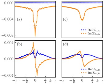
As long as , are kept small and , the sample data shown here is representative of the agreement between Eq. (11) and the CSBA result, meaning that there is always some deviation around that can be mitigated by a finite .
Appendix E Symmetries of GFs at general complex argument
The Källén–Lehmann representation of the GF can be written in terms of eigenvectors of the full Hamiltonian ,
| ((12)) |
where the weights have the symmetry . In general, complex conjugation leads to
which in matrix notation reads , or
| ((13)) |
E.1 Time-Reversal Symmetry
Under TRS, fermionic operators transform as
where repeated indices are implicitly summed over [82]. If the Hamiltonian is invariant under time-reversal, i.e. , the application of to an eigenstate yields a (possibly different) eigenstate with the same energy: . Since is anti-unitary, we have where denotes the unitary part. Anti-unitarity by definition implies and thus . For any two eigenstates of a TRS-invariant Hamiltonian, it follows that for any operator . If the Hamiltonian is invariant under time-reversal, we can then rewrite Eq. (12) as
which in matrix notation reads , or equivalently .
E.2 Particle-Hole Symmetry
PHS is a unitary symmetry under which fermionic operators transform as [82]
Assuming invariance of the Hamiltonian under PHS implies that is an eigenstate with the same energy, and the GF becomes
which can be written as .
E.3 Chiral Symmetry
Under CS, the combination of TRS and PHS, fermionic operators transform as [82]
Since is also anti-unitary, we once again have with some unitary part . The unitary transformation matrix is related to the ones representing TRS and PHS via . The GF thus satisfies
which is equivalent to or, via Eq. (13), .
E.4 Summary
To summarize, assuming the respective symmetry, the GF for general complex satisfies
| TRS | ((14)) | |||||
| PHS | ((15)) | |||||
| CS | ((16)) |
or any equivalent forms obtained by inserting the symmetry-independent result from Eq. (13) (i.e. ). At zero temperature, the same symmetry constraints have already been derived by [83]. The translation to the Matsubara GF is trivial by replacing . For the real time GF, Eq. (13) yields . Then, CS for the retarded GF can be obtained by , which gives .
References
- Note [1] Tomonaga-Luttinger Liquids [6, 27, 30, 63, 64, 38] (or even Landau-Luttinger Liquids [4]), originate from the Tomonaga-Luttinger model [84, 85, 5, 23, 69, 86, 9, 10, 13, 29] and are often simply referred to as Luttinger Liquids [2, 69, 8, 9, 13, 29] in analogy to Landau’s Fermi Liquid [87, 14, 88, 4, 5, 89, 23, 69, 8, 16].
- Haldane [1981] F. D. M. Haldane, Effective harmonic-fluid approach to low-energy properties of one-dimensional quantum fluids, Phys. Rev. Lett. 47, 1840 (1981).
- Shankar [1994] R. Shankar, Renormalization-group approach to interacting fermions, Reviews of Modern Physics 66, 129–192 (1994).
- Voit [1995] J. Voit, One-dimensional fermi liquids, Reports on Progress in Physics 58, 977 (1995).
- Schulz [1995] H. J. Schulz, Fermi liquids and non-fermi liquids, in Mesoscopic Quantum Physics, edited by E. A. et al. (Elsevier, Amsterdam, 1995) pp. 533–592.
- von Delft and Schoeller [1998] J. von Delft and H. Schoeller, Bosonization for beginners — refermionization for experts, Annalen der Physik 510, 225 (1998).
- Gogolin et al. [1999a] A. O. Gogolin, A. A. Nersesyan, and A. M. Tsvelik, Bosonization and strongly correlated systems (1999a), arXiv:cond-mat/9909069 [cond-mat.str-el] .
- Rao and Sen [2001] S. Rao and D. Sen, An introduction to bosonization and some of its applications, in Field Theories in Condensed Matter Physics (Hindustan Book Agency, Gurgaon, 2001) pp. 239–333.
- Bowen and Gulácsi [2001] G. Bowen and M. Gulácsi, Finite-temperature bosonization, Philosophical Magazine B 81, 1409 (2001).
- Schonhammer [2003] K. Schonhammer, Luttinger liquids: The basic concepts (2003), arXiv:cond-mat/0305035 [cond-mat.str-el] .
- Miranda [2003] E. Miranda, Introduction to bosonization, Brazilian Journal of Physics 33, 3 (2003).
- Giamarchi [2004] T. Giamarchi, Quantum physics in one dimension, International series of monographs on physics (Clarendon Press, Oxford, 2004).
- Sénéchal [2004] D. Sénéchal, An introduction to bosonization, in Theoretical Methods for Strongly Correlated Electrons, edited by D. Sénéchal, A.-M. Tremblay, and C. Bourbonnais (Springer New York, New York, NY, 2004) pp. 139–186.
- Landau [1957a] L. D. Landau, Oscillations in a fermi liquid, JETP 5, 101 (1957a).
- Qian and Vignale [2005] Z. Qian and G. Vignale, Lifetime of a quasiparticle in an electron liquid, Phys. Rev. B 71, 075112 (2005).
- Vignale [2022] G. Vignale, Fermi liquids, in Dynamical mean-field theory of correlated electrons lecture notes of the Autumn School on Correlated Electrons 2022, edited by A. L. E. Pavarini, E. Koch and D. Vollhardt (Forschungszentrum Jülich GmbH, Institute for Advanced Simulation, Jülich, 2022) pp. 53–92.
- Gornyi et al. [2005] I. V. Gornyi, A. D. Mirlin, and D. G. Polyakov, Dephasing and weak localization in disordered luttinger liquid, Phys. Rev. Lett. 95, 046404 (2005).
- Le Hur [2006] K. Le Hur, Electron lifetime in luttinger liquids, Phys. Rev. B 74, 165104 (2006).
- Giamarchi and Schulz [1988] T. Giamarchi and H. J. Schulz, Anderson localization and interactions in one-dimensional metals, Phys. Rev. B 37, 325 (1988).
- Wen [1990] X. G. Wen, Chiral luttinger liquid and the edge excitations in the fractional quantum hall states, Phys. Rev. B 41, 12838 (1990).
- Nersesyan et al. [1993] A. Nersesyan, A. Luther, and F. Kusmartsev, Scaling properties of the two-chain model, Physics Letters A 176, 363 (1993).
- Schulz [1996] H. J. Schulz, Phases of two coupled luttinger liquids, Phys. Rev. B 53, R2959 (1996).
- Mattsson et al. [1997] A. E. Mattsson, S. Eggert, and H. Johannesson, Properties of a Luttinger liquid with boundaries at finite temperature and size, Physical Review B 56, 15615 (1997).
- Capponi et al. [2000] S. Capponi, D. Poilblanc, and T. Giamarchi, Effects of long-range electronic interactions on a one-dimensional electron system, Phys. Rev. B 61, 13410 (2000).
- Wu et al. [2003] C. Wu, W. Vincent Liu, and E. Fradkin, Competing orders in coupled luttinger liquids, Phys. Rev. B 68, 115104 (2003).
- Dolcini et al. [2005] F. Dolcini, B. Trauzettel, I. Safi, and H. Grabert, Transport properties of single-channel quantum wires with an impurity: Influence of finite length and temperature on average current and noise, Phys. Rev. B 71, 165309 (2005).
- Furusaki [2005] A. Furusaki, Kondo problems in tomonaga-luttinger liquids, Journal of the Physical Society of Japan 74, 73 (2005).
- Imambekov et al. [2008] A. Imambekov, V. Gritsev, and E. Demler, Mapping of coulomb gases and sine-gordon models to statistics of random surfaces, Phys. Rev. A 77, 063606 (2008).
- Grap and Meden [2009] S. Grap and V. Meden, Renormalization-group study of luttinger liquids with boundaries, Phys. Rev. B 80, 193106 (2009).
- Furukawa and Kim [2010] S. Furukawa and Y. Kim, Entanglement entropy between two coupled tomonaga-luttinger liquids, Physical Review B 83 (2010).
- Ström et al. [2010] A. Ström, H. Johannesson, and G. I. Japaridze, Edge dynamics in a quantum spin hall state: Effects from rashba spin-orbit interaction, Phys. Rev. Lett. 104, 256804 (2010).
- Budich et al. [2012] J. C. Budich, F. Dolcini, P. Recher, and B. Trauzettel, Phonon-induced backscattering in helical edge states, Phys. Rev. Lett. 108, 086602 (2012).
- Crépin et al. [2012] F. Crépin, J. C. Budich, F. Dolcini, P. Recher, and B. Trauzettel, Renormalization group approach for the scattering off a single rashba impurity in a helical liquid, Phys. Rev. B 86, 121106 (2012).
- Japaridze et al. [2013] G. Japaridze, H. Johannesson, and M. Malard, Synthetic helical liquid in a quantum wire, Physical Review B 89 (2013).
- Schmidt and Pedder [2016] T. L. Schmidt and C. J. Pedder, Helical gaps in interacting rashba wires at low electron densities, Phys. Rev. B 94, 125420 (2016).
- Rylands and Andrei [2016] C. Rylands and N. Andrei, Quantum impurity in a luttinger liquid: Exact solution of the kane-fisher model, Phys. Rev. B 94, 115142 (2016).
- Jin et al. [2023] T. Jin, P. Ruggiero, and T. Giamarchi, Bosonization of the interacting su-schrieffer-heeger model, Phys. Rev. B 107, L201111 (2023).
- Gohlke et al. [2024] M. Gohlke, J. C. Pelayo, and T. Suzuki, Proximate tomonaga-luttinger liquid in an anisotropic kitaev-gamma model, Phys. Rev. B 109, L220410 (2024).
- Rudner and Levitov [2009] M. S. Rudner and L. S. Levitov, Topological transition in a non-hermitian quantum walk, Phys. Rev. Lett. 102, 065703 (2009).
- Lee [2016] T. E. Lee, Anomalous edge state in a non-hermitian lattice, Phys. Rev. Lett. 116, 133903 (2016).
- Lieu [2018] S. Lieu, Topological phases in the non-hermitian su-schrieffer-heeger model, Phys. Rev. B 97, 045106 (2018).
- Gong et al. [2018] Z. Gong, Y. Ashida, K. Kawabata, K. Takasan, S. Higashikawa, and M. Ueda, Topological phases of non-hermitian systems, Phys. Rev. X 8, 031079 (2018).
- Budich et al. [2019] J. C. Budich, J. Carlström, F. K. Kunst, and E. J. Bergholtz, Symmetry-protected nodal phases in non-hermitian systems, Phys. Rev. B 99, 041406 (2019).
- Luitz and Piazza [2019] D. J. Luitz and F. Piazza, Exceptional points and the topology of quantum many-body spectra, Phys. Rev. Res. 1, 033051 (2019).
- Yoshida et al. [2019] T. Yoshida, R. Peters, N. Kawakami, and Y. Hatsugai, Symmetry-protected exceptional rings in two-dimensional correlated systems with chiral symmetry, Phys. Rev. B 99, 121101 (2019).
- Budich and Bergholtz [2020] J. C. Budich and E. J. Bergholtz, Non-hermitian topological sensors, Phys. Rev. Lett. 125, 180403 (2020).
- Okuma et al. [2020] N. Okuma, K. Kawabata, K. Shiozaki, and M. Sato, Topological origin of non-hermitian skin effects, Phys. Rev. Lett. 124, 086801 (2020).
- Lin et al. [2023] R. Lin, T. Tai, L. Li, and C. H. Lee, Topological non-hermitian skin effect, Frontiers of Physics 18, 53605 (2023).
- Micallo et al. [2023] T. Micallo, C. Lehmann, and J. C. Budich, Correlation-induced sensitivity and non-hermitian skin effect of quasiparticles, Phys. Rev. Res. 5, 043105 (2023).
- Berry [2004] M. V. Berry, Physics of nonhermitian degeneracies, Czechoslovak Journal of Physics 54, 1039 (2004).
- Heiss [2012] W. D. Heiss, The physics of exceptional points, Journal of Physics A: Mathematical and Theoretical 45, 444016 (2012).
- Kozii and Fu [2024] V. Kozii and L. Fu, Non-hermitian topological theory of finite-lifetime quasiparticles: Prediction of bulk fermi arc due to exceptional point, Phys. Rev. B 109, 235139 (2024).
- Yuto Ashida and Ueda [2020] Z. G. Yuto Ashida and M. Ueda, Non-hermitian physics, Advances in Physics 69, 249 (2020), https://doi.org/10.1080/00018732.2021.1876991 .
- Bergholtz et al. [2021] E. J. Bergholtz, J. C. Budich, and F. K. Kunst, Exceptional topology of non-hermitian systems, Rev. Mod. Phys. 93, 015005 (2021).
- Rausch et al. [2021] R. Rausch, R. Peters, and T. Yoshida, Exceptional points in the one-dimensional hubbard model, New Journal of Physics 23, 013011 (2021).
- Lehmann et al. [2021] C. Lehmann, M. Schüler, and J. C. Budich, Dynamically induced exceptional phases in quenched interacting semimetals, Phys. Rev. Lett. 127, 106601 (2021).
- Michen et al. [2021] B. Michen, T. Micallo, and J. C. Budich, Exceptional non-hermitian phases in disordered quantum wires, Phys. Rev. B 104, 035413 (2021).
- Eek et al. [2024] L. Eek, A. Moustaj, M. Röntgen, V. Pagneux, V. Achilleos, and C. M. Smith, Emergent non-hermitian models, Phys. Rev. B 109, 045122 (2024).
- Ashida et al. [2017] Y. Ashida, S. Furukawa, and M. Ueda, Parity-time-symmetric quantum critical phenomena, Nature Communications 8, 15791 (2017).
- Dóra and Moca [2020] B. Dóra and C. P. Moca, Quantum quench in -symmetric luttinger liquid, Phys. Rev. Lett. 124, 136802 (2020).
- Dubey et al. [2023] A. Dubey, S. Biswas, and A. Kundu, Operator correlations in a quenched non-hermitian luttinger liquid, Phys. Rev. B 108, 085433 (2023).
- Nakagawa et al. [2021] M. Nakagawa, N. Kawakami, and M. Ueda, Exact liouvillian spectrum of a one-dimensional dissipative hubbard model, Phys. Rev. Lett. 126, 110404 (2021).
- Yamamoto et al. [2022] K. Yamamoto, M. Nakagawa, M. Tezuka, M. Ueda, and N. Kawakami, Universal properties of dissipative tomonaga-luttinger liquids: Case study of a non-hermitian xxz spin chain, Phys. Rev. B 105, 205125 (2022).
- Yamamoto and Kawakami [2023] K. Yamamoto and N. Kawakami, Universal description of dissipative tomonaga-luttinger liquids with spin symmetry: Exact spectrum and critical exponents, Phys. Rev. B 107, 045110 (2023).
- Su et al. [1979] W. P. Su, J. R. Schrieffer, and A. J. Heeger, Solitons in polyacetylene, Phys. Rev. Lett. 42, 1698 (1979).
- Heeger et al. [1988] A. J. Heeger, S. Kivelson, J. R. Schrieffer, and W. P. Su, Solitons in conducting polymers, Rev. Mod. Phys. 60, 781 (1988).
- Note [2] This is essentially the kinetic part of the Tomonaga-Luttinger model [90, 10].
- Malard et al. [2015] M. Malard, G. Japaridze, and H. Johannesson, Synthesizing majorana zero-energy modes in a periodically gated quantum wire, Physical Review B 94, 115128 (2015).
- Schulz et al. [1998] H. J. Schulz, G. Cuniberti, and P. Pieri, Fermi liquids and luttinger liquids, in Field Theories for Low-Dimensional Condensed Matter Systems: Spin Systems and Strongly Correlated Electrons, edited by G. Morandi, P. Sodano, A. Tagliacozzo, and V. Tognetti (Springer Berlin Heidelberg, Berlin, Heidelberg, 1998) pp. 9–81.
- Gogolin et al. [1999b] A. O. Gogolin, A. A. Nersesyan, and A. M. Tsvelik, Bosonization and Strongly Correlated Systems (1999) arXiv:cond-mat/9909069 [cond-mat.str-el] .
- Fradkin [2013] E. Fradkin, Field Theories of Condensed Matter Physics, 2nd ed. (Cambridge University Press, 2013).
- Altland and Simons [2010] A. Altland and B. D. Simons, Condensed matter field theory (Cambridge University Press, 2010).
- Delamotte [2012] B. Delamotte, An introduction to the nonperturbative renormalization group, in Renormalization Group and Effective Field Theory Approaches to Many-Body Systems, edited by A. Schwenk and J. Polonyi (Springer Berlin Heidelberg, Berlin, Heidelberg, 2012) pp. 49–132.
- Eder [2021] R. Eder, Green functions and self-energy functionals, in Simulating correlations with computers Lecture notes of the autumn school on correlated electrons 2021, edited by E. Pavarini and E. Koch (Forschungszentrum Jülich GmbH, Institute for Advanced Simulation, Jülich, 2021) pp. 175–199.
- Note [3] Note that we have the general result for non-singular matrices.
- Note [4] for .
- [77] N. Dupuis, Field Theory Of Condensed Matter And Ultracold Gases – Volume 2 (to be published in 2025, see https://www.lptmc.jussieu.fr/users/dupuis).
- Collins [1984] J. C. Collins, Renormalization: An Introduction to Renormalization, the Renormalization Group and the Operator-Product Expansion, 1st ed. (Cambridge University Press, 1984).
- Note [5] Note that, if the integrals converge, is the result from with . A sharp cut-off instead leads to and the indeterminate limit .
- Bruus and Flensberg [2004] H. Bruus and K. Flensberg, Many-Body Quantum Theory in Condensed Matter Physics: An Introduction (Oxford University Press, 2004).
- Puig von Friesen et al. [2010] M. Puig von Friesen, C. Verdozzi, and C.-O. Almbladh, Kadanoff-baym dynamics of hubbard clusters: Performance of many-body schemes, correlation-induced damping and multiple steady and quasi-steady states, Phys. Rev. B 82, 155108 (2010).
- Chiu et al. [2016] C.-K. Chiu, J. C. Teo, A. P. Schnyder, and S. Ryu, Classification of topological quantum matter with symmetries, Reviews of Modern Physics 88, 035005 (2016).
- Gurarie [2011] V. Gurarie, Single-particle green’s functions and interacting topological insulators, Phys. Rev. B 83, 085426 (2011).
- Tomonaga [1950] S.-i. Tomonaga, Remarks on bloch’s method of sound waves applied to many-fermion problems, Progress of Theoretical Physics 5, 544 (1950).
- Luttinger [1963] J. M. Luttinger, An exactly soluble model of a many-fermion system, Journal of Mathematical Physics 4, 1154 (1963).
- Castellani and Di Castro [1999] C. Castellani and C. Di Castro, Breakdown of fermi liquid in correlated electron systems, Physica A: Statistical Mechanics and its Applications 263, 197 (1999), proceedings of the 20th IUPAP International Conference on Statistical Physics.
- Landau [1957b] L. D. Landau, The theory of a fermi liquid, JETP 3, 920 (1957b).
- Luttinger and Nozières [1962] J. M. Luttinger and P. Nozières, Derivation of the landau theory of fermi liquids. ii. equilibrium properties and transport equation, Phys. Rev. 127, 1431 (1962).
- Neilson [1996] D. Neilson, Landau fermi liquid theory, Australian journal of physics 49, 79 (1996).
- Mattis and Lieb [1965] D. C. Mattis and E. H. Lieb, Exact solution of a many-fermion system and its associated boson field, Journal of Mathematical Physics 6, 304 (1965).