Krylov complexity of purification

Abstract

Purification maps a mixed state to a pure state and a non-unitary evolution into a unitary one by enlarging the Hilbert space. We link the operator complexity of the density matrix to the state/operator complexity of purified states using three purification schemes: time-independent, time-dependent, and instantaneous purification. We propose inequalities among the operator and state complexities of mixed states and their purifications, demonstrated with a single qubit, two-qubit Werner states, and infinite-dimensional diagonal mixed states. We find that the complexity of a vacuum evolving into a thermal state equals the average number of Rindler particles created between left and right Rindler wedges. Finally, for the thermofield double state evolving from zero to finite temperature, we show that 1) the state complexity follows the Lloyd bound, reminiscent of the quantum speed limit, and 2) the Krylov state/operator complexities are subadditive in contrast to the holographic volume complexity.

Introduction.—

The study of information-theoretic quantities in physics has led to fascinating discoveries in various contexts ranging from quantum many-body systems to quantum gravity [1, 2, 3, 4, 5, 6, 7, 8, 9]. In recent years, there has been significant interest in open quantum systems, where a pure system entangles with the environment. From the system’s point of view, a pure state turns into a mixed state due to the coupling. This non-unitary nature poses significant challenges and impacts various fields including quantum phases of mixed states [10, 11, 9], noisy quantum computation [12, 13, 14], the Unruh effect [15, 16], the black hole information paradox [17, 18, 19, 20], and inflating universes [21, 22, 23, 24, 25, 26, 27]. Although these systems experience non-unitary evolution, incorporating the environment renders the dynamics unitary in an extended Hilbert space—a process known as purification.

Purification-related quantities, such as the entanglement of purification (EoP) [28] and reflected entropy [29, 30, 31, 32], offer valuable insights into the entanglement structure of mixed states. However, establishing a quantitative relationship between the measures of the system’s mixed state and those of the purified state is often complicated; for instance, EoP bounds bipartite entanglement measures of mixed states, including the squashed entanglement [33], but they could be largely different [34]. Therefore, it is essential to clarify the relationship between mixed-state measures and those of the purifications for a deeper understanding of mixed states.

The complexity of quantum systems describes how quantum states or operators become complex over time. Krylov operator complexity, a measure initially developed to study operator growth in the Heisenberg picture during unitary evolution [35], evaluates this complexity. This concept was parallelly extended to the Schrödinger evolution of pure quantum states, known as spread complexity, which measures how an initial pure state disperses under unitary evolution governed by the system’s Hamiltonian [36]. This concept has also been adapted to non-unitary evolution in open quantum systems [37, 38, 39, 40, 41, 42, 43, 44].

In this letter, we propose a novel framework to study the Krylov operator complexity of mixed states through the spread state and Krylov operator complexities of their purifications. Our approach offers a unified method to understand complexity growth in both pure and mixed states, overcoming a gap in current methodologies. Purifying a density matrix ensures that the purified state undergoes a unitary evolution in the extended Hilbert space. Our complexity of purification (CoP) in Krylov space extends the concept previously studied for Nielsen, circuit, and holographic complexities [45, 46, 47, 48, 49, 50, 51, 52, 53, 54, 55, 56, 57, 58, 59, 60, 61], but differs in that we do not require CoP minimized over all purifications. Rather we leave their non-uniqueness for probing various aspects of the mixed-state complexity.

We explore three purification schemes: time-independent, time-dependent, and instantaneous purification. They exhibit different time evolutions on the ancilla and hence different complexity growths while describing the same mixed-state evolution after tracing out the ancilla. This variety of purifications leads to bounds among complexity measures before and after purification. We demonstrate these bounds with unitarily evolving two-qubit Werner states and non-unitarily evolving infinite-dimensional Gaussian mixed states, which are identified with a thermal state with varying temperatures in time. By identifying the latter system with the Minkowski vacuum in the Rindler frame, we provide a quasiparticle picture accounting for the difference in the prefactor between the original complexity and CoP. Finally, we demonstrate that the spread complexity of purification (CoP) for the thermal state is bounded above by the product of entropy and temperature, in agreement with the Lloyd bound [62]. To investigate the subadditivity property of Krylov complexities, we introduce a new quantity, which we term mutual Krylov complexity. We show that Krylov complexity is subadditive for the thermofield double (TFD) state, contrary to the holographic complexity based on the complexity$=$volume (CV) and CV2.0 proposal [63, 64, 65, 7, 66, 67, 68].

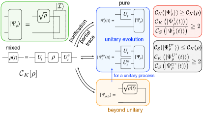
Figure 1: Graphical visualization of purification schemes using circuit diagrams. The top left box shows the purified state $\ket{\psi_{\rho}}$ for the mixed density matrix $\rho$. The central blue and orange boxes illustrate how the time evolution of $\rho(t)$ is reflected in the pure state through the choice of purification. The rightmost boxes highlight the bounds for mixed and purification complexities.

Definitions.—

We start by reviewing the definitions of the Krylov complexity for a density matrix and the spread complexity for a pure state. For a detailed discussion, refer to Appendix I in the Supplemental Material. Let us consider a density matrix $\rho(t)$ that follows the Liouville-von Neumann equation, $\rho(t)=e^{-iHt}\,\rho(0)\,e^{iHt}$ . Using the Baker-Campbell-Hausdorff formula $\rho(t)$ can be written as the sum of nested commutators of $H$ and $\rho(0)$. By making a choice of the inner product, say, $\left(\rho_{1}|\rho_{2}\right):=\text{Tr}\left[\rho_{1}^{\dagger}\rho_{2}\right]$ and using the Lanczos algorithm on the set of operators the nested commutators, we obtain the Krylov basis $|\phi_{n})$. The time-dependent density matrix $\rho(t)$ can be expanded in the Krylov basis $|\rho(t))=\sum_{n}i^{n}\varphi_{n}(t)|\phi_{n})$, where the probability amplitudes $\varphi_{n}(t)$ satisfy $\sum|\varphi_{n}(t)|^{2}=1$. This leads to the definition of the Krylov operator complexity $\mathcal{C}_{K}$ of the operator $\rho(t)$,

$$\begin{split}\mathcal{C}_{K}(t):=\sum_{n}n\left|\varphi_{n}(t)\right|^{2}.\end{split}$$ (1)

Krylov complexity can alternatively be calculated from the autocorrelation function $(\rho(t)|\rho(0))$ [70].

The spread complexity (also known as the Krylov state complexity) is the optimal measure of complexity that quantifies the spread of a pure state as it evolves [36]. Starting with an initial state $|\psi(0)\rangle$ along with the Schrödinger evolution, $|\psi(t)\rangle=e^{-iHt}|\psi(0)\rangle,$ the Krylov basis $|K_{n}\rangle$ can be built from the set of states $\{H^{n}|\psi(0)\rangle,n\in\mathbb{Z}\}$ by using the Lanczos algorithm as reviewed in Appendix I in the Supplemental Material. Expanding the time-evolved state in the Krylov basis leads to $|\psi(t)\rangle=\sum_{n}\psi_{n}(t)|K_{n}\rangle$. Here, $|\psi_{n}(t)|^{2}$ represents the probability of the state being in the $n$-th Krylov basis element $|K_{n}\rangle$ at time $t$, with total probability $\sum_{n}|\psi_{n}(t)|^{2}=1$. The spread complexity $\mathcal{C}_{S}$ of a pure state $\ket{\psi(t)}$ is defined as the average position in the Krylov space of states

$$\mathcal{C}_{S}(t)=\sum_{n}n|\psi_{n}(t)|^{2}.$$ (2)

Now, let us discuss three distinct purification schemes. Before purification, the operator complexity is the sole option, aside from pure states. However, once purified, both the state and operator complexities can be examined for the purified states. Given a density matrix $\rho$ of a system $S$, its purification is generically written as $\ket{\Psi_{\rho}^{V}}_{SA}=(\rho^{1/2}\otimes V_{R\rightarrow A})\ket{\mathcal{I}}_{SR}$, where $V$ is an isometry from $R$ to $A$, i.e. $V^{\dagger}V=\mathbf{1}_{R}$, and $\ket{\mathcal{I}}_{SR}=\sum_{n=1}^{\rank\rho}\ket{n}_{S}\otimes\ket{n}_{R}$ is an unnormalized EPR state [71, 72, 73]. For $\rho$ evolving unitarily by $U_{t}=e^{-iHt}$, the purification evolves as $\ket{\Psi_{\rho}^{V}(t)}=(U_{t}\rho^{1/2}\otimes V(t))\ket{\mathcal{I}}=(U_{t}\otimes V(t))\ket{\Psi_{\rho}}$, where $\ket{\Psi_{\rho}}:=|\Psi_{\rho}^{\mathbb{I}}\rangle$. Note that $\ket{\Psi_{\rho}}$ is the initial purification with the minimal dimension. It differs from the canonical purification [74] unless $\rho$ is full-rank. We emphasize that any choice of $V(t)$ results in the same time evolution $\rho\mapsto\rho(t)=U_{t}\rho U_{t}^{\dagger}$ for the initial system.

One possible choice for the isometry is $V(t)=\mathbb{I}$ and we refer to this as time-independent purification. The time-evolved purified state is denoted by

$$\ket{\Psi^{\mathbb{I}}_{\rho}(t)}=(U_{t}\otimes\mathbb{I})\ket{\Psi_{\rho}}.$$ (3)

Alternatively, we can choose a time-dependent isometry $V(t)$. Choosing $V(t)=U_{t}^{\ast}$, we define the the time-dependent purification after time $t$ becomes

$$\ket{\Psi^{U^{\ast}}_{\rho}(t)}=(U_{t}\rho^{1/2}U_{t}^{\dagger}\otimes\mathbb{I})\ket{\mathcal{I}}=(U_{t}\otimes U_{t}^{\ast})\ket{\Psi_{\rho}}.$$ (4)

This is motivated by considering a static state $\rho\propto\mathbb{I}$ and requiring the purification to be also static.

Lastly, instantaneous purification is defined as the purification of the density matrix at each moment. The purified state at time $t$ is given by

$$\ket{\Psi_{\rho(t)}}:=(\rho(t)^{1/2}\otimes\mathbb{I})\ket{\mathcal{I}}.$$ (5)

This purification also applies when $\rho$ evolves non-unitarily, in which case a pure state may evolve into a mixed state. Instantaneous purification reduces to time-dependent purification for a unitary evolution.

We do not require minimization over purification unlike previous proposals of the circuit CoP, however, our definition of CoPs is optimal under certain assumptions. For time-independent isometry, the Krylov/spread complexities are unaffected by the isometry choice, as its dependence cancels out in the autocorrelation function. For time-dependent isometry, we can always fix the dimension of the Hilbert space as time evolves by preparing a sufficiently large number of ancilla. This implies the isometry can be decomposed as $V(t)=W(t)V_{0}$, where $V_{0}$ is time-independent, and $W(t)$ is a time-dependent unitary. For the CoP to approximate the original complexity well, we need CoP to be zero when the original complexity is zero (no time evolution), requiring $W(t)V_{0}=W_{0}U_{t}^{\ast}$, with $W_{0}$ an arbitrary time-independent isometry. As the upper bound of complexity grows with dimension [75], the smallest complexity is likely to be achieved by the smallest purification. Setting $V_{0}=W_{0}=\mathbb{I}$ gives the time-dependent purification (4). A similar argument leads to the instantaneous purification (5).

The three different purification schemes enable us to define both the Krylov complexity (1) of the purified state through its density matrix form but also the spread complexity (2) through its state vector form .

Inequalities among complexities.—

Based on the three types of purifications defined above, we conjecture inequalities for the complexities of mixed states and their purifications, with analytical and numerical evidence provided in the later section.

1. Krylov operator complexity of the mixed state is upper bounded by the operator complexity of the time-independent purification and is lower bounded by the state complexity of the time-dependent purification,

   $$\mathcal{C}_{K}\quantity(\ket{\Psi_{\rho}^{\mathbb{I}}(t)})\geq\mathcal{C}_{K}(\rho(t))\geq\mathcal{C}_{S}\quantity(\ket{\Psi_{\rho}^{U^{\ast}}(t)})$$ (6)

   where the equality holds in the pure state limit.

2. The ratio of the state complexity of the time-dependent purification and the operator complexity of the original mixed state, $\mathcal{C}_{S}(\ket{\Psi_{\rho}^{U^{\ast}}(t)})/\mathcal{C}_{K}(\rho(t))$, is approximately constant and its value depends on the purity of $\rho$; the temporal average of the ratio equals a constant $\leq 1$.

3. For the same type of purification scheme, the CoPs satisfy $\mathcal{C}_{K}\quantity(\ket{\Psi_{\rho}^{U^{\ast},\mathbb{I}}(t)})\geq 2\mathcal{C}_{S}\quantity(\ket{\Psi_{\rho}^{U^{\ast},\mathbb{I}}(t)})$.

4. The Krylov and spread complexity of the time-independent purification, $\mathcal{C}_{S,K}(\ket{\Psi_{\rho}^{\mathbb{I}}(t)}$, are weakly sensitive to the purity of the initial density matrix $\Tr(\rho^{2}(t=0))$.

Examples.—

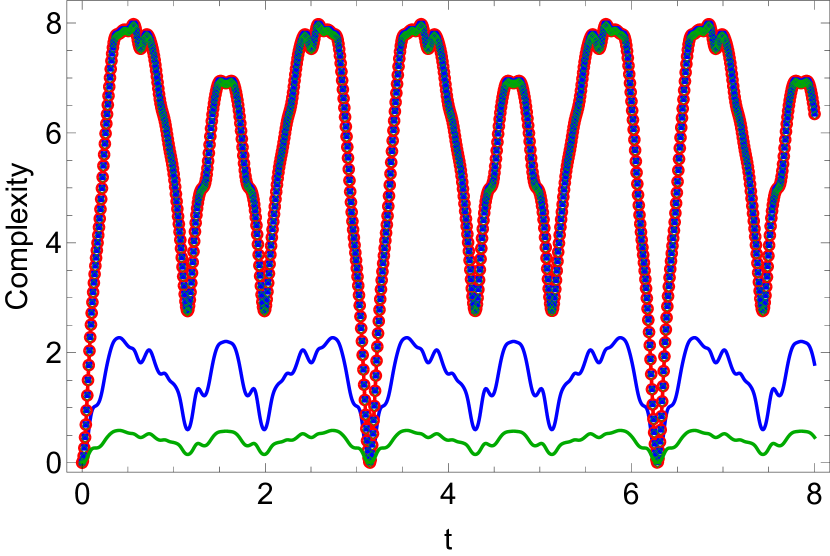
(a)

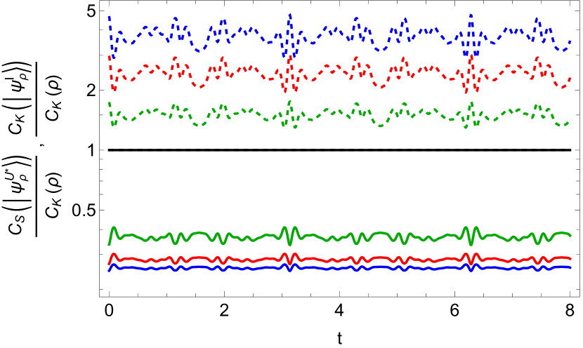
(b)

(c)

Figure 2: Time dependence of the complexities of the Werner states (7) with $r=4$ and $q=15$ in the Hamiltonian (8). (a) Each complexity $\mathcal{C}_{K}(|\Psi_{\rho}^{\mathbb{I}}(t)\rangle)$ (red), $\mathcal{C}_{K}(\rho(t))$ (blue), and $\mathcal{C}_{S}(|\Psi_{\rho}^{U^{\ast}}(t)\rangle)$ (green) for different parameters $p=1/4$ (solid curve) and $p\rightarrow 1$ (dotted points). Every complexity coincides for $p\rightarrow 1$, and $\mathcal{C}_{K}(|\Psi_{\rho}^{\mathbb{I}}(t)\rangle)$ overlaps among different $p$. (b) Ratio between the operator complexity and CoPs: $\mathcal{C}_{K}(|\Psi_{\rho}^{\mathbb{I}}(t)\rangle)/\mathcal{C}_{K}(\rho(t))$ (dashed curve) and $\mathcal{C}_{S}(|\Psi_{\rho}^{U^{\ast}}(t)\rangle)/\mathcal{C}_{K}(\rho(t))$ (solid curve) for $p=1/4$ (blue), $p=1/3$ (red), $p=1/2$ (green), and $p\rightarrow 1$ (black) in log scale. (c) Ratio $\mathcal{C}_{K}/\mathcal{C}_{S}$ between the state and operator CoPs for the time-independent purification (dashed curve) and the time-dependent purification (solid curve) for $p=1/4$ (blue) and $p\rightarrow 1$ (red) with a reference line at $2$ (black).

We first study the CoPs for the two-qubit Werner states and demonstrate the proposed bounds. The two-qubit Werner state is defined as

$$\rho=\frac{p}{2}(\ket{01}-\ket{10})(\bra{01}-\bra{10})+\frac{1-p}{4}\mathbb{I}_{4\times 4}.$$ (7)

The parameter $p$ interpolates between the maximally mixed state $\rho\propto\mathbb{I}$ at $p=0$ and a pure, maximally entangled state $\ket{Y}\equiv(\ket{01}-\ket{10})/\sqrt{2}$ at $p=1$. Additionally, the state is separable for $p\leq\frac{1}{3}$ and entangled otherwise. Since the Werner state commutes with the Pauli matrices $\sigma_{i}\otimes\sigma_{i}$ for any $i=x,y,z$, let us consider the following Hamiltonian for a nontrivial time evolution:

$$H=\mathbf{\sigma}_{x}\otimes\mathbf{\sigma}_{y}+r\,\mathbf{\sigma}_{y}\otimes\mathbf{\sigma}_{z}+q\,\mathbf{\sigma}_{z}\otimes\mathbf{\sigma}_{x},$$ (8)

where $r$ and $q$ are free parameters. For the time-independent and time-dependent purification, the evolution is governed by $H\otimes\mathbb{I}$ and $H\otimes\mathbb{I}-\mathbb{I}\otimes H^{*}$, respectively. While the coefficients of each term in the Hamiltonian (8) is not unique, we keep them different from each other to prevent additional symmetries. For Fig. 2, we choose $r=4$ and $q=15$. For other choices of parameters, see Appendix III of the Supplemental Material.

As we are interested in the mixed-state complexity, we focus on $0\leq p<1$. As the $\rho$ is always full-rank, the initial state for the CoPs is given by the canonical purification, namely, $|\Psi_{\rho}\rangle=\sqrt{\frac{1+p}{4}}\ket{YY}+\sqrt{\frac{1-p}{4}}(\ket{II}+\ket{XX}+\ket{ZZ}),$ where $\ket{I},\ket{X},\ket{Y},\ket{Z}$ are the Bell basis [73].

Fig. 2(a) shows that the operator complexity of the original mixed state $\mathcal{C}_{K}(\rho(t))$, shown in blue, is bounded by CoPs. Two choices of initial states are presented by solid ($p=1/4$) and dotted ($p\rightarrow 1$) lines. The recurrence time [77, 78] is common and the operator complexity of the time-independent purification $\mathcal{C}_{K}(\ket{\psi_{\rho}^{\mathbb{I}}(t)})$ (red) bounds $\mathcal{C}_{K}(\rho(t))$ from above and the state complexity of the time-dependent purification $\mathcal{C}_{S}(\ket{\psi_{\rho}^{U^{*}}(t)})$ (green) bounds it from below. The inequalities (6) are saturated in the limit $p\rightarrow 1$, which can be thought as a manifestation of the doubled Hilbert space via purification .

We also highlight that in Fig. 2(a) initial states with different purities have the same $\mathcal{C}_{K}(|\Psi_{\rho(t)}^{\mathbb{I}}\rangle)$ as long as the Hamiltonian is the same. This demonstrates the fourth property mentioned earlier. We also confirm this for $\mathcal{C}_{S}(|\Psi_{\rho(t)}^{\mathbb{I}}\rangle)$. This insensitivity to the initial states suggests that the complexity of time-independent purification is a more robust probe of the features of the system evolution compared to other Krylov complexities.

Fig. 2(b) shows the time-dependence of the ratio of CoPs to the original mixed-state complexity $\mathcal{C}_{K}(\rho(t))$. This plot demonstrates the second property: the operator complexity of the original mixed state is approximately proportional to the state complexity of the time-dependent purification, whose proportionality constant depends on purity. For more quantitative analysis on its fluctuation, refer to Appendix IV in the Supplemental material. This property particularly aligns with our initial motivation to find CoP, such that it provides insights into the operator complexity of the original mixed states. Comparing the ratio of CoPs to unity, Fig. 2(b) further demonstrates the inequalities (6).

In Fig. 2(c), we show that for the same type of purification of the Werner state, $\mathcal{C}_{K}(t)\geq 2\mathcal{C}_{S}(t)$ always holds regardless of the choice of initial states. This property extends a previous observation of $\mathcal{C}_{K}=2\mathcal{C}_{S}$ for maximally entangled states [80] to the inequality for pure states . We conjecture the property $\mathcal{C}_{K}\geq 2\mathcal{C}_{S}$ is true in general. It can be confirmed analytically for an arbitrary qubit with an arbitrary time evolution. See Appendix II in the Supplemental Material for more details.

Next, let us apply our framework to a non-unitarily evolving infinite-dimensional diagonal mixed state

$$\rho(r)=\frac{1}{\cosh^{2}r}\sum_{n=0}^{\infty}\tanh^{2n}r\outerproduct{n}{n}.$$ (9)

We model a non-unitary evolution by taking a time-dependent $r=\alpha t$ so that it interpolates a pure state at $t=0$ and the maximally mixed state at $t\rightarrow\infty$. The instantaneous purification of (9) is given by a two-mode squeezed vacuum (TMSV):

$$\ket{\Psi_{\rho(r)}}=\frac{1}{\cosh r}\sum_{n=0}^{\infty}(-i\tanh r)^{n}\ket{n}\ket{n}$$ (10)

as long as $\rho(r)$ is mixed, equivalently $r>0$. As $r$ is linear in time, (10) is generated by a two-mode squeezing Hamiltonian $H=\alpha(ab+a^{\dagger}b^{\dagger})$ on a separable pure state $\ket{00}$ defined in the enlarged Hilbert space [82, 83, 49]. $a$ ($a^{\dagger}$) and $b$ ($b^{\dagger}$) are the annihilation (creation) operators acting on the system and the ancilla, respectively.

In the following, we denote the original mixed state at time $t$ by $\rho(t)$. Since the evolution is non-unitary, we can consider either the operator complexity of the original mixed state (9) and the operator/state complexity of its instantaneous purification (10). For $\mathcal{C}_{K}(\rho(t))$, the autocorrelation function is given by $\Tr(\rho(t)\rho(0))$ and for $\mathcal{C}_{K}(|\Psi_{\rho(t)}\rangle)$, it is given by $[\Tr(\rho^{1/2}(t)\rho^{1/2}(0))]^{2}$. They are both equal to $\sech^{2}(\alpha t)$ . Thus, their Krylov complexities are also identical. The Krylov complexity with this autocorrelation function is given by [35, 85]

$$\mathcal{C}_{K}(\rho(t))=\mathcal{C}_{K}\quantity(\ket{\Psi_{\rho(t)}})=2\sinh^{2}(\alpha t).$$ (11)

The spread complexity of the instantaneous purification (10) is easily calculated by the Gaussian nature of the TMSV [86]. It follows from the Krylov basis being the number basis that

$$\mathcal{C}_{S}(\ket{\Psi_{\rho(t)}})=\expectationvalue{n}=\sinh^{2}(\alpha t).$$ (12)

Both $\mathcal{C}_{K}(\rho(t))$ and $\mathcal{C}_{S}(\ket{\Psi_{\rho(t)}})$ exhibit exponential growth with the same exponent, up to a factor of two.

The above results show that CoPs capture key features of the Krylov complexity of the original non-unitary evolution, extending our conjecture $\mathcal{C}_{K}(\ket{\Psi})\geq 2\mathcal{C}_{S}(\ket{\Psi})$ and $\mathcal{C}_{S}[\ket{\Psi}]\leq\mathcal{C}_{K}(\rho)$ to non-unitary cases. Moreover, computing spread CoP is typically easier than computing the original Krylov complexity. For example, by utilizing the translational invariance of the spread complexity [87], one can easily find that the spread CoP for the initially mixed state (9) with $r=r_{0}$ is given by $\sinh^{2}(\alpha t-r_{0})$. As no analytical form for the operator complexity is known from its autocorrelation function, it demonstrates an advantage of our proposal of CoP.

In fact, the mixed state (9) and its purification (10) can be identified as a Gibbs and TFD state of a harmonic oscillator, respectively . The parameter $r$ is related to the inverse temperature $\beta$ via $\tanh^{2}r=e^{-\beta\Delta E}$, where $\Delta E$ is the energy spacing. With this identification, we can correspond (10) with the mode expansion of the two-dimensional Minkowski vacuum of a massless free field in terms of the left (L) and right (R) Rindler basis.

Based on this identification, let us give a quasiparticle interpretation to (12). The complexity of the vacuum state $\mathcal{C}_{S}(|\Psi_{\rho(t)}\rangle)$ grows by exchanging the Rindler particles between two Rindler wedges. Then, the growth rate (12) is naturally given by the average number of the exchanged quasiparticles. The same argument applies for a perturbation falling into a black hole . By exchanging one Hawking quanta between the exterior and its interior partner, the state thermalizes and the spread complexity increases by one. The quasiparticle picture also explains the factor $2$ of $\mathcal{C}_{K}(\rho(t))$ in (11). Since the original mixed state only sees one Rindler wedge, both the absorption and emission happen simultaneously. This increases the complexity by two per unit of time.

Following [90], we can define another complexity for the subsystem. Provided the subsystem spread operator given by $K_{L}=\Tr_{R}\sum_{n}n\outerproduct{n_{L}n_{R}}{n_{L}n_{R}}=\sum_{n}n\outerproduct{n}{n}_{L}$, the subsystem spread complexity for $L$ is given by

$$\mathcal{C}^{L}_{S}(\rho(t))=\Tr(K_{L}\rho_{L}(t))=\sinh^{2}(\alpha t).$$ (13)

The equality with the spread CoP is explained in the quasiparticle picture as follows. Because the spread operator is only defined in one subsystem, the effect of the incoming quanta is excluded, and the subsystem complexity grows by the outgoing quanta.

Finally, we highlight a relation between the spread CoP and thermodynamic quantities. The time derivative of the spread CoP (12) and the energy $E$ and the von Neumann entropy $S$ of (9) at time $t$, i.e. thermal energy and entropy of temperature $T=-\Delta E/\log\tanh^{2}(\alpha t)$, satisfy

$$\dot{\mathcal{C}}_{S}:=\derivative{\mathcal{C}_{S}(|\Psi_{\rho(t)}\rangle)}{t}\leq\frac{\alpha}{\Delta E}2E,\quad\dot{\mathcal{C}}_{S}\leq\frac{\alpha}{\Delta E}TS.$$ (14)

This reminds us of the Lloyd bound [62] of the complexity. Without characteristic scales other than $\Delta E$, we take the time scale $\alpha\sim\Delta E$. Thus, (14) simplifies to $\dot{\mathcal{C}}_{S}\lesssim E,\dot{\mathcal{C}}_{S}\lesssim TS$, aligning with the Lloyd bound of holographic complexity from the CV proposal [63, 64, 65, 7, 66, 67, 60]. The first bound in (14) saturates at the late time as in the case of black holes. The bound of (14) is reminiscent of the quantum speed limit on Krylov complexity growth [91, 42, 92], suggesting that the Lloyd bound may serve as the speed limit for spread complexity.

Despite the similarity of the Lloyd bound, we find that the operator complexity and CoPs in the Krylov formalism differ from the holographic ones based on CV/CV2.0 proposals. To demonstrate this, let us introduce the mutual Krylov complexity for a bipartite state $\rho_{AB}$ as This quantity itself has been introduced in the context of the Nielsen and holographic complexities [93, 54],

$$\Delta\mathcal{C}(A:B)=\mathcal{C}(\rho_{A}(t))+\mathcal{C}(\rho_{B}(t))-\mathcal{C}(\rho_{AB}(t)).$$ (15)

Possible choices For the complexity measure $\mathcal{C}$ are the Krylov operator complexity, the subsystem complexity, and the operator/state CoPs. For the TFD case, we have $\Delta\mathcal{C}(L:R)=2\mathcal{C}(\rho(t))-\mathcal{C}(|\Psi_{\rho(t)}\rangle)$. Following (11), (12), and (13), the mutual Krylov complexity $\Delta\mathcal{C}(L:R)$ equals $2\sinh^{2}(\alpha t)$ for the operator complexity/CoP ($\mathcal{C}=\mathcal{C}_{K}$) in (15) and $\sinh^{2}(\alpha t)$ for the state complexity/CoP ($\mathcal{C}=\mathcal{C}_{S}$) in (15) . In all cases, the operator complexity and state/operator CoPs show subadditivity, $\Delta\mathcal{C}(L:R)\geq 0$, in contrast to superadditivity of holographic complexity observed in the CV and CV2.0 proposals [54, 45, 95, 96, 53]. As the present calculation is based on the free field $E_{n}\propto n$, further holographic CFT computations are needed to confirm the discrepancy between mutual Krylov and holographic complexities.

Conclusion.—

In this study, we put forward the complexity of purification in Krylov formalism. We explore three distinct purification schemes applicable to both unitary and non-unitary evolutions. Various bounds are conjectured among the original complexity and both the spread and Krylov CoPs. These inequalities are demonstrated with two-qubit Werner states undergoing a unitary evolution. The relation $\mathcal{C}_{K}\geq 2\mathcal{C}_{S}$ for pure states is further analytically confirmed with a generic single-qubit state. The spread complexity of time-dependent purification resembles the Krylov complexity of the mixed state, yet CoP is simpler to evaluate. Furthermore, we apply CoP to an infinite-dimensional thermal state with increasing temperature. We find this non-unitary case also satisfies the proposed inequalities by saturating them. We present a consistent quasiparticle picture based on the Rindler frame, which is also applicable for a perturbation falling into a black hole. Finally, we observe that the spread complexity adheres to the Lloyd bound. However, we show that Krylov complexities in our setup differ from holographic ones based on CV or CV2.0 conjectures because of the subadditive nature of Krylov complexities. While further analytical evidence for the conjectured properties remains to be explored, our CoPs proposal enables convenient and coherent probing of the complexity of mixed states and non-unitary evolution.

Supplemental Material

I Krylov and Spread complexity

Spread Complexity

In this subsection, we summarize the key concepts necessary to measure the complexity associated with the spreading of a quantum state and the evolution of an operator in the Krylov space for systems governed by Hermitian Hamiltonians [70]. For state complexity, we begin with a pure state, with unitary dynamics ensuring that the state remains pure during evolution. For such a quantum system governed by the Hamiltonian $H$, the spread (state) complexity can be defined. Consider a time-evolved state $|\psi(t)\rangle=e^{-iHt}|\psi(0)\rangle$. This can be written as a linear combination of

$$|\psi\rangle,~{}H|\psi\rangle,~{}H^{2}|\psi\rangle,~{}\cdots,$$ (S.1)

where $|\psi(0)\rangle$ is denoted as $|\psi\rangle$. The subspace $\mathcal{H}_{|\psi\rangle}$ spanned by (S.1) is known as the Krylov space. Using the natural inner product, we can orthonormalize (S.1) using the Lanczos algorithm:

• $b_{0}\equiv 0$,

• $|K_{0}\rangle\equiv|\psi(0)\rangle,a_{0}=\langle K_{0}|H|K_{0}\rangle$

• For $n\geq 1$: $|\mathcal{A}_{n}\rangle=(H-a_{n-1})|K_{n-1}\rangle-b_{n-1}|K_{n-2}\rangle$

• Set $b_{n}=\sqrt{\langle\mathcal{A}_{n}|\mathcal{A}_{n}\rangle}$

• If $b_{n}=0$, stop; otherwise, set $|K_{n}\rangle=\frac{1}{b_{n}}|\mathcal{A}_{n}\rangle,a_{n}=\langle K_{n}|H|K_{n}\rangle$, and repeat step 3.

If $\mathcal{D}\equiv\dim\mathcal{H}_{|\psi\rangle}$ is finite, the Lanczos algorithm concludes with $b_{\mathcal{D}}=0$. The resulting orthonormal basis $\{|K_{n}\rangle\}_{n=0}^{\mathcal{D}-1}$ is called the Krylov basis. Note that there are two sets of Lanczos coefficients $\{a_{n}\}$ and $\{b_{n}\}$ in this context. Expressing $|\psi(t)\rangle$ in terms of the Krylov basis yields

$$|\psi(t)\rangle=\sum_{n=0}^{\mathcal{D}-1}\psi_{n}(t)|K_{n}\rangle,$$ (S.2)

and substituting (S.2) into the Schrödinger equation, we obtain

$$i\dot{\psi}_{n}(t)=a_{n}\psi_{n}(t)+b_{n+1}\psi_{n+1}(t)+b_{n}\psi_{n-1}(t).$$ (S.3)

The initial condition is $\psi_{n}(0)=\delta_{n0}$ by definition. Importantly, the weights $\psi_{n}$ of each Krylov basis element $|K_{n}\rangle$ can be interpreted as a wave function with support on a semi-infinite chain.

The (Krylov) state complexity is the extent to which the state has spread along the chain, or equivalently, the number of Krylov basis elements it encompasses. More precisely, the spread complexity of the state $|\psi\rangle$ is defined as

$$\mathcal{C}_{S}(t)\equiv\sum_{n=0}^{\mathcal{D}-1}n|\psi_{n}(t)|^{2}.$$ (S.4)

As intuitively expected, this notion of complexity serves as a probe for chaos. Note, however, that chaos will manifest differently in state spread complexity compared to (operator) Krylov complexity, as suggested by the conjecture in [35]. Typically, the spread of states in a Hilbert space, as opposed to operators, will display a distinct signature for chaos.

Krylov Operator Complexity

In this subsection, we review Krylov operator complexity [70]. Consider a quantum system evolving under the Hamiltonian $H$. In the Heisenberg picture, the Krylov complexity for an operator $\mathcal{O}$ is defined as follows. The time-evolved operator $\mathcal{O}(t)=e^{iHt}\mathcal{O}(0)e^{-iHt}$ can be expanded as

$$\mathcal{O}(t)=\sum_{n=0}^{\infty}\frac{(it)^{n}}{n!}\mathcal{L}^{n}\mathcal{O}(0),$$ (S.5)

where $\mathcal{L}$ is the Liouvillian superoperator, given by $\mathcal{L}=[H,\cdot]$. This is a superposition of the following operators:

$$\mathcal{O},\mathcal{L}\mathcal{O},\mathcal{L}^{2}\mathcal{O},\cdots,$$ (S.6)

where $\mathcal{O}$ represents $\mathcal{O}(0)$. The space $\mathcal{H}_{\mathcal{O}}$ spanned by (S.6) is termed the Krylov space associated with $\mathcal{O}$. By introducing an inner product between operators $\mathcal{O}_{1}$ and $\mathcal{O}_{2}$ as, for example,

$$(\mathcal{O}_{1}|\mathcal{O}_{2})\equiv{\rm Tr}\big{[}\mathcal{O}_{1}^{\dagger}\mathcal{O}_{2}\big{]},$$ (S.7)

we can construct an orthonormal basis for $\mathcal{H}_{\mathcal{O}}$ using the Lanczos algorithm:

• $b_{0}\equiv 0,\quad\mathcal{O}_{-1}\equiv 0$

• $\mathcal{O}_{0}\equiv\mathcal{O}/|\mathcal{O}|$, where $|\mathcal{O}|\equiv\sqrt{(\mathcal{O}|\mathcal{O})}$

• For $n\geq 1$: $\mathcal{A}_{n}=\mathcal{L}\mathcal{O}_{n-1}-b_{n-1}\mathcal{O}_{n-2}$

• Set $b_{n}=|\mathcal{A}_{n}|$

• If $b_{n}=0$, stop; otherwise, set $\mathcal{O}_{n}=\mathcal{A}_{n}/b_{n}$ and repeat step 3.

In finite-dimensional systems, the Lanczos algorithm terminates with $b_{K_{\mathcal{O}}}=0$, where $K_{\mathcal{O}}\equiv\dim\mathcal{H}_{\mathcal{O}}$. This yields the orthonormal basis $\{\mathcal{O}_{n}\}_{n=0}^{K_{\mathcal{O}}-1}$ termed the Krylov basis, and positive numbers $\{b_{n}\}$ known as the Lanczos coefficients. Expanding the Heisenberg operator $\mathcal{O}(t)$ in terms of the Krylov basis gives

$$\mathcal{O}(t)=\sum_{n=0}^{K_{\mathcal{O}}-1}i^{n}\varphi_{n}(t)\mathcal{O}_{n},$$ (S.8)

where $\varphi_{n}(t)$ satisfies the normalization condition

$$\sum_{n=0}^{K_{\mathcal{O}}-1}|\varphi_{n}(t)|^{2}=|\mathcal{O}|^{2}=1$$ (S.9)

after correctly normalizing the initial operator $\mathcal{O}$. Substituting (S.8) into the Heisenberg equation leads to

$$\dot{\varphi}_{n}(t)=b_{n}\varphi_{n-1}(t)-b_{n+1}\varphi_{n+1}(t),$$ (S.10)

where the dot represents the derivative with respect to time. The initial condition is $\varphi_{n}(0)=\delta_{n0}|\mathcal{O}|$ by definition, which simplifies to $\varphi_{n}(0)=\delta_{n0}$ after normalizing the operator. The Krylov complexity for the operator $\mathcal{O}$ is defined as

$$\mathcal{C}_{\mathcal{O}}(t)\equiv\sum_{n=0}^{K_{\mathcal{O}}-1}n|\varphi_{n}(t)|^{2}.$$ (S.11)

The operator $\mathcal{O}_{n}$ includes the nested commutator $\mathcal{L}^{n}\mathcal{O}$, which generally becomes more complex as $n$ increases. Thus, Krylov operator complexity quantifies the number of nested commutators in the Heisenberg operator $\mathcal{O}(t)$. Both Krylov and the spread complexity can also be computed from the autocorrelation function and the return amplitude, respectively. For the details, refer to the following review [70].

II Proof of $\mathcal{C}_{K}\geq 2\,\mathcal{C}_{S}$ for an arbitrary qubit with an arbitrary time evolution

As discussed in [80], the Krylov operator complexity of a pure qubit $\rho=\outerproduct{\psi}{\psi}$ such that

$$\ket{\psi}=\cos\theta\ket{E_{1}}+\sin\theta e^{i\phi}\ket{E_{2}},$$ (S.12)

under an arbitrary time evolution generated by the Hamiltonian $H=E_{1}\outerproduct{E_{1}}{E_{1}}+E_{2}\outerproduct{E_{2}}{E_{2}}$ is given by

$$\mathcal{C}_{K}(\ket{\psi(t)})=\frac{1}{2}\sin^{2}(2\theta)\quantity(\sin^{2}\tau+2(3+\cos(4\theta))\sin^{4}\frac{\tau}{2}),$$ (S.13)

where we defined a dimensionless time parameter $\tau=\Delta E\,t$.

The spread state complexity of $\rho$ is given by

$$\mathcal{C}_{S}(\ket{\psi(t)})=\sin^{2}(2\theta)\sin^{2}\frac{\tau}{2}.$$ (S.14)

Its ratio is calculated as

$$\frac{\mathcal{C}_{K}(\ket{\psi(t)})}{2\mathcal{C}_{S}(\ket{\psi(t)})}=1+\cos^{2}(2\theta)\sin^{2}\frac{\tau}{2}\geq 1.$$ (S.15)

This confirms the inequality $\mathcal{C}_{K}\geq 2\,\mathcal{C}_{S}$ for an arbitrary one-qubit pure state under an arbitrary unitary evolution.

III Mixed state and purified state complexity for different parameters

As the fourth property of the purification complexity, we have mentioned that the complexity of time-independent purification, $\mathcal{C}_{S,K}(\ket{\psi\rho^{\mathbb{I}}(t)})$, are almost insensitive to the purity of the initial state. As we can see in Fig. 3, in practice, $\mathcal{C}_{S,K}(\ket{\psi\rho^{\mathbb{I}}(t)})$ overlaps for different values of purity of the initial state. This makes them a better probe for understanding the dynamical properties of the Hamiltonian. In the case of Werner state purification, the system is still just a four-qubit system, and the dynamics is very simple. Here, we show that the state/operator complexity of time-independent purification does indeed change for different parameters of the Hamiltonian but not for the different initial states. We propose for future studies that the complexity of time-independent purification could be used as a diagnostic for the time evolution, e.g. chaotic Hamiltonians exhibiting the transition from integrable to chaotic behaviour.

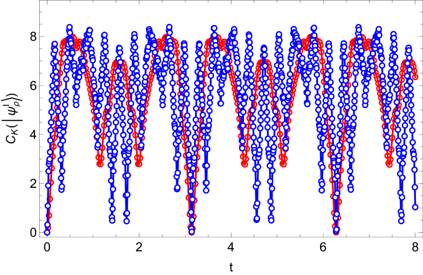
(a) Krylov complexity of time-independent purification

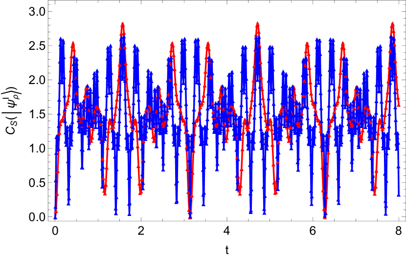
(b) Spread complexity of time-independent purification

Figure 3: In both panels, the red color signifies the Hamiltonian parameters of (8) with $r=4$ and $q=15$, while the blue color signifies the Hamiltonian parameters with $r=10$ and $q=50$. (a) The empty circles, in both red and blue, signify the purified state with $p\rightarrow 1$, and the solid lines signify $p=1/4$ for the initial state (7). (b) The solid triangles, in both red and blue, signify the purified state with $p\rightarrow 1$, and the solid lines signify $p=1/4$. For both the operator and the state complexity, the complexity overlaps for the different purity parameters with the same Hamiltonian but differs for different Hamiltonian parameters.

IV Relation between $\mathcal{C}_{K}(\rho)/\mathcal{C}_{S}(|\Psi_{\rho}^{U^{\ast}}\rangle)$ and the purity of the initial mixed state

Following (6), the value of $\mathcal{C}_{K}(\rho)$ is lower bounded by $\mathcal{C}_{S}\quantity(\ket{\Psi_{\rho}^{U^{\ast}}})$ and they behave quite similarly. In this part, we discuss the initial state dependence of the ratio $\mathcal{C}_{K}(\rho)/\mathcal{C}_{S}\quantity(\ket{\Psi_{\rho}^{U^{\ast}}})$ is mostly given by the purity $\Tr\rho^{2}$ . (Notice that the ratio considered in this section is the inverse of the ratio plotted in Fig. 2(c).) In Fig. 4(a), we plot

$$R(\rho(t)):=\frac{\mathcal{C}_{K}(\rho(t))}{\mathcal{C}_{S}\quantity(\ket{\Psi_{\rho}^{U^{\ast}}(t)})}\times\Tr(\rho^{2})$$ (S.16)

as a function of time. We find that the ratio of the complexities, $R(\rho)$, is inversely proportional to the purity of the initial state up to small fluctuations. This can be also seen from its temporal average over the recurrence time [77, 78], when complexity returns to zero, as shown in Fig. 4(b).

(a)

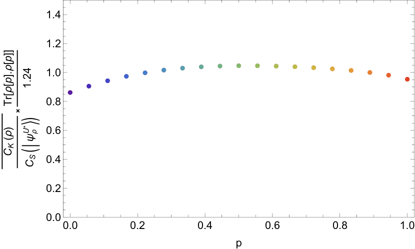
(b)

Figure 4: The central legend bar showing different values of the parameter $p$ is common to both of the panels. The Hamiltonian (8) with $r=4$ and $q=15$ has been used to generate these results.                                                                                                                                                   (a) Time evolution of $R(\rho(t))$ for different values of purity of the initial state for the density matrix given by (7). $R(\rho(t))$ is concentrated around a particular range which shows that $\mathcal{C}_{K}(\rho(t))/\mathcal{C}_{S}\quantity(\ket{\Psi_{\rho}^{U^{\ast}}(t)})$ is proportional to the inverse of the purity of the initial density matrix up to fluctuations.                                                                                                                                                   (b) Variation of the time average of the ratio times purity, $\overline{\mathcal{C}_{K}(\rho(t))/\mathcal{C}_{S}\quantity(\ket{\Psi_{\rho}^{U^{\ast}}(t)})}\times\Tr(\rho^{2})$ with purity of the initial mixed density matrix. The horizontal axis is scaled by a constant factor of $1/1.24$.

Figure 5: The fluctuation in the ratio of the complexities, $\mathcal{C}_{K}(\rho)/\mathcal{C}_{S}\quantity(\ket{\Psi_{\rho}^{U^{\ast}}})$. The column ”Mean Ratio” is the time average of $\mathcal{C}_{K}(\rho)/\mathcal{C}_{S}\quantity(\ket{\Psi_{\rho}^{U^{\ast}}})$ over the period of recurrence time scale.

Fig. 5 lists various measures for the fluctuations of the ratio of complexities $\mathcal{C}_{K}(\rho)/\mathcal{C}_{S}(|\Psi_{\rho}^{U^{\ast}}\rangle)$ with different values of the parameter $p$ in the Werner state (7). We find that numerically, the state complexity of the time-dependent purification and the operator complexity of the original mixed states agree with each other reasonably well. For a quantitative evaluation, let us look at the coefficient of variation. In the current case, it is defined as the standard deviation over time divided by the average ratio over recurrence time. Fig. 5 shows that the coefficient of variation is below 5%, indicating the concentration around a constant value.

References

- Calabrese and Cardy [2009] P. Calabrese and J. Cardy, J. Phys. A 42, 504005 (2009), arXiv:0905.4013 [cond-mat.stat-mech] .
- Casini and Huerta [2009] H. Casini and M. Huerta, J. Phys. A 42, 504007 (2009), arXiv:0905.2562 [hep-th] .
- Augusiak et al. [2012] R. Augusiak, F. M. Cucchietti, and M. Lewenstein, “Many-body physics from a quantum information perspective,” in Lecture Notes in Physics (Springer Berlin Heidelberg, 2012) p. 245–294.
- Laflorencie [2016] N. Laflorencie, Physics Reports 646, 1–59 (2016).
- Harlow [2016] D. Harlow, Rev. Mod. Phys. 88, 015002 (2016), arXiv:1409.1231 [hep-th] .
- Rangamani and Takayanagi [2017] M. Rangamani and T. Takayanagi, Holographic Entanglement Entropy (Springer International Publishing, 2017).
- Susskind [2018] L. Susskind (Springer, 2018) arXiv:1810.11563 [hep-th] .
- Headrick [2019] M. Headrick, (2019), arXiv:1907.08126 [hep-th] .
- Sang et al. [2023] S. Sang, Y. Zou, and T. H. Hsieh, (2023), arXiv:2310.08639 [quant-ph] .
- Verstraete et al. [2009] F. Verstraete, M. M. Wolf, and J. Ignacio Cirac, Nature Physics 5, 633 (2009), arXiv:0803.1447 [quant-ph] .
- Diehl et al. [2008] S. Diehl, A. Micheli, A. Kantian, B. Kraus, H. P. Büchler, and P. Zoller, Nature Physics 4, 878 (2008), arXiv:0803.1482 [quant-ph] .
- Preskill [2018] J. Preskill, Quantum 2, 79 (2018), arXiv:1801.00862 [quant-ph] .
- Noh et al. [2020] K. Noh, L. Jiang, and B. Fefferman, Quantum 4, 318 (2020), arXiv:2003.13163 [quant-ph] .
- Li et al. [2023] Z. Li, S. Sang, and T. H. Hsieh, Phys. Rev. B 107, 014307 (2023), arXiv:2203.16555 [quant-ph] .
- Unruh [1976] W. G. Unruh, Phys. Rev. D 14, 870 (1976).
- Crispino et al. [2008] L. C. B. Crispino, A. Higuchi, and G. E. A. Matsas, Rev. Mod. Phys. 80, 787 (2008), arXiv:0710.5373 [gr-qc] .
- Hawking [1976] S. W. Hawking, Phys. Rev. D 14, 2460 (1976).
- Hawking [1974] S. W. Hawking, Nature 248, 30 (1974).
- Hawking [1975] S. W. Hawking, Commun. Math. Phys. 43, 199 (1975), [Erratum: Commun.Math.Phys. 46, 206 (1976)].
- Page [1993] D. N. Page, Phys. Rev. Lett. 71, 3743 (1993), arXiv:hep-th/9306083 .
- Dong et al. [2018] X. Dong, E. Silverstein, and G. Torroba, JHEP 07, 050 (2018), arXiv:1804.08623 [hep-th] .
- Shaghoulian [2022] E. Shaghoulian, JHEP 01, 132 (2022), arXiv:2110.13210 [hep-th] .
- Shaghoulian and Susskind [2022] E. Shaghoulian and L. Susskind, JHEP 08, 198 (2022), arXiv:2201.03603 [hep-th] .
- Chandrasekaran et al. [2023] V. Chandrasekaran, R. Longo, G. Penington, and E. Witten, JHEP 02, 082 (2023), arXiv:2206.10780 [hep-th] .
- Witten [2024] E. Witten, Proc. Symp. Pure Math. 107, 247 (2024), arXiv:2303.02837 [hep-th] .
- Shaghoulian [2023] E. Shaghoulian, (2023), arXiv:2305.10635 [hep-th] .
- Balasubramanian et al. [2024a] V. Balasubramanian, Y. Nomura, and T. Ugajin, JHEP 02, 135 (2024a), arXiv:2308.09748 [hep-th] .
- Terhal et al. [2002] B. M. Terhal, M. Horodecki, D. W. Leung, and D. P. DiVincenzo, J. Math. Phys. 43, 4286 (2002), arXiv:quant-ph/0202044 .
- Bao and Cheng [2019] N. Bao and N. Cheng, JHEP 10, 102 (2019), arXiv:1909.03154 [hep-th] .
- Chu et al. [2020] J. Chu, R. Qi, and Y. Zhou, JHEP 03, 151 (2020), arXiv:1909.10456 [hep-th] .
- Bueno and Casini [2020a] P. Bueno and H. Casini, JHEP 05, 103 (2020a), arXiv:2003.09546 [hep-th] .
- Bueno and Casini [2020b] P. Bueno and H. Casini, JHEP 11, 148 (2020b), arXiv:2008.11373 [hep-th] .
- Christandl and Winter [2004] M. Christandl and A. Winter, J. Math. Phys. 45, 829 (2004).
- Umemoto and Zhou [2018] K. Umemoto and Y. Zhou, Journal of High Energy Physics 2018 (2018), 10.1007/jhep10(2018)152.
- Parker et al. [2019] D. E. Parker, X. Cao, A. Avdoshkin, T. Scaffidi, and E. Altman, Phys. Rev. X 9, 041017 (2019), arXiv:1812.08657 [cond-mat.stat-mech] .
- Balasubramanian et al. [2022] V. Balasubramanian, P. Caputa, J. M. Magan, and Q. Wu, Phys. Rev. D 106, 046007 (2022), arXiv:2202.06957 [hep-th] .
- Bhattacharya et al. [2022a] A. Bhattacharya, P. Nandy, P. P. Nath, and H. Sahu, JHEP 12, 081 (2022a), arXiv:2207.05347 [quant-ph] .
- Bhattacharya et al. [2023a] A. Bhattacharya, R. N. Das, B. Dey, and J. Erdmenger, “Spread complexity for measurement-induced non-unitary dynamics and Zeno effect,” (2023a), arXiv:2312.11635 [hep-th] .
- Bhattacharjee et al. [2023] B. Bhattacharjee, X. Cao, P. Nandy, and T. Pathak, JHEP 03, 054 (2023), arXiv:2212.06180 [quant-ph] .
- Bhattacharya et al. [2023b] A. Bhattacharya, P. Nandy, P. P. Nath, and H. Sahu, JHEP 12, 066 (2023b), arXiv:2303.04175 [quant-ph] .
- Bhattacharjee et al. [2024] B. Bhattacharjee, P. Nandy, and T. Pathak, JHEP 01, 094 (2024), arXiv:2311.00753 [quant-ph] .
- Bhattacharya et al. [2024a] A. Bhattacharya, P. P. Nath, and H. Sahu, Phys. Rev. D 109, L121902 (2024a), arXiv:2403.03584 [quant-ph] .
- Bhattacharya et al. [2024b] A. Bhattacharya, R. N. Das, B. Dey, and J. Erdmenger, (2024b), arXiv:2406.03524 [hep-th] .
- Nandy et al. [2024a] P. Nandy, T. Pathak, and M. Tezuka, (2024a), arXiv:2406.11969 [quant-ph] .
- Agón et al. [2019] C. A. Agón, M. Headrick, and B. Swingle, Journal of High Energy Physics 2019 (2019), 10.1007/jhep02(2019)145.
- Camargo et al. [2019] H. A. Camargo, P. Caputa, D. Das, M. P. Heller, and R. Jefferson, Physical Review Letters 122 (2019), 10.1103/physrevlett.122.081601.
- Ghodrati et al. [2019] M. Ghodrati, X.-M. Kuang, B. Wang, C.-Y. Zhang, and Y.-T. Zhou, JHEP 09, 009 (2019), arXiv:1902.02475 [hep-th] .
- Camargo et al. [2021] H. A. Camargo, L. Hackl, M. P. Heller, A. Jahn, T. Takayanagi, and B. Windt, Phys. Rev. Res. 3, 013248 (2021), arXiv:2009.11881 [hep-th] .
- Haque et al. [2022] S. S. Haque, C. Jana, and B. Underwood, JHEP 01, 159 (2022), arXiv:2107.08969 [hep-th] .
- Bhattacharya et al. [2022b] A. Bhattacharya, A. Bhattacharyya, and S. Maulik, Phys. Rev. D 106, 086010 (2022b), arXiv:2209.00049 [hep-th] .
- Bhattacharyya et al. [2024] A. Bhattacharyya, S. Brahma, S. S. Haque, J. S. Lund, and A. Paul, JHEP 05, 058 (2024), arXiv:2401.12134 [hep-th] .
- Bhattacharyya et al. [2022] A. Bhattacharyya, T. Hanif, S. S. Haque, and M. K. Rahman, Phys. Rev. D 105, 046011 (2022), arXiv:2112.03955 [hep-th] .
- Cáceres et al. [2019] E. Cáceres, J. Couch, S. Eccles, and W. Fischler, Phys. Rev. D 99, 086016 (2019), arXiv:1811.10650 [hep-th] .
- Caceres et al. [2020] E. Caceres, S. Chapman, J. D. Couch, J. P. Hernandez, R. C. Myers, and S.-M. Ruan, JHEP 03, 012 (2020), arXiv:1909.10557 [hep-th] .
- Ruan [2021a] S.-M. Ruan, JHEP 01, 092 (2021a), arXiv:2006.01088 [hep-th] .
- Di Giulio and Tonni [2020] G. Di Giulio and E. Tonni, JHEP 12, 101 (2020), arXiv:2006.00921 [hep-th] .
- Di Giulio [2021] G. Di Giulio, Circuit complexity and entanglement in many-body quantum systems, Ph.D. thesis, SISSA, Trieste (2021).
- Chapman and Policastro [2022] S. Chapman and G. Policastro, Eur. Phys. J. C 82, 128 (2022), arXiv:2110.14672 [hep-th] .
- Bhattacharya et al. [2021] A. Bhattacharya, A. Bhattacharyya, P. Nandy, and A. K. Patra, Journal of High Energy Physics 2021 (2021), 10.1007/jhep05(2021)135.
- Yang et al. [2019] R.-Q. Yang, H.-S. Jeong, C. Niu, and K.-Y. Kim, JHEP 04, 146 (2019), arXiv:1902.07586 [hep-th] .
- Wang et al. [2023] D. Wang, X. Qiao, M. Wang, Q. Pan, C. Lai, and J. Jing, Nucl. Phys. B 991, 116223 (2023), arXiv:2301.00513 [hep-th] .
- Lloyd [2000] S. Lloyd, Nature 406, 1047 (2000), arXiv:quant-ph/9908043 [quant-ph] .
- Brown et al. [2016] A. R. Brown, D. A. Roberts, L. Susskind, B. Swingle, and Y. Zhao, Phys. Rev. D 93, 086006 (2016), arXiv:1512.04993 [hep-th] .
- Carmi et al. [2017] D. Carmi, S. Chapman, H. Marrochio, R. C. Myers, and S. Sugishita, JHEP 11, 188 (2017), arXiv:1709.10184 [hep-th] .
- Susskind [2016] L. Susskind, Fortsch. Phys. 64, 24 (2016), [Addendum: Fortsch.Phys. 64, 44–48 (2016)], arXiv:1403.5695 [hep-th] .
- Yang [2020] R.-Q. Yang, Phys. Rev. D 102, 106001 (2020), arXiv:1911.12561 [hep-th] .
- Engelhardt and Folkestad [2022] N. Engelhardt and r. Folkestad, JHEP 01, 040 (2022), arXiv:2109.06883 [hep-th] .
- Couch et al. [2017] J. Couch, W. Fischler, and P. H. Nguyen, JHEP 03, 119 (2017), arXiv:1610.02038 [hep-th] .
- Note [1] Note that the sign of the evolution arises from the state evolution, contrasting with the Heisenberg operator evolution commonly considered in the Krylov operator complexity.
- Nandy et al. [2024b] P. Nandy, A. S. Matsoukas-Roubeas, P. Martínez-Azcona, A. Dymarsky, and A. del Campo, (2024b), arXiv:2405.09628 [quant-ph] .
- Wilde [2011] M. M. Wilde, (2011), 10.1017/9781316809976.001, arXiv:1106.1445 [quant-ph] .
- Wilde [2017] M. M. Wilde, Quantum Information Theory, 2nd ed. (Cambridge University Press, 2017).
- Nielsen and Chuang [2012] M. A. Nielsen and I. L. Chuang, Quantum Computation and Quantum Information: 10th Anniversary Edition (Cambridge University Press, 2012).
- Dutta and Faulkner [2021] S. Dutta and T. Faulkner, JHEP 03, 178 (2021), arXiv:1905.00577 [hep-th] .
- Rabinovici et al. [2020] E. Rabinovici, A. Sánchez-Garrido, R. Shir, and J. Sonner, (2020), arXiv:2009.01862 [hep-th] .
- Note [2] Notice the difference in normalization with [90]. In [90], a density matrix is mapped to a vector by the Choi-Jamiołkowski isomorphism, so it needs additional normalization by . In our definition of CoPs, we do not need any such normalization once the initial state is normalized as .
- Balasubramanian et al. [2024b] V. Balasubramanian, R. N. Das, J. Erdmenger, and Z.-Y. Xian, (2024b), arXiv:2407.11114 [hep-th] .
- Hashimoto et al. [2023] K. Hashimoto, K. Murata, N. Tanahashi, and R. Watanabe, JHEP 11, 040 (2023), arXiv:2305.16669 [hep-th] .
- Note [3] The equality between and for pure states can be seen from the matching of the autocorrelation function.
- Caputa et al. [2024] P. Caputa, H.-S. Jeong, S. Liu, J. F. Pedraza, and L.-C. Qu, “Krylov complexity of density matrix operators,” (2024), arXiv:2402.09522 [hep-th] .
- Note [4] Note that even when the initial state is maximally entangled (), it is only within the two-dimensional subspace. Thus, this does not mean a contradiction to the observation in [80].
- Caves and Schumaker [1985] C. M. Caves and B. L. Schumaker, Phys. Rev. A 31, 3068 (1985).
- Ou et al. [1992] Z. Y. Ou, S. F. Pereira, H. J. Kimble, and K. C. Peng, Phys. Rev. Lett. 68, 3663 (1992).
- Note [5] Interestingly, the scaling of the autocorrelation function in our example matches with that of the low- Sachdev-Ye-Kitaev model in the decoupling limit (). Here corresponds to .
- Caputa et al. [2022] P. Caputa, J. M. Magan, and D. Patramanis, Phys. Rev. Res. 4, 013041 (2022), arXiv:2109.03824 [hep-th] .
- Adhikari et al. [2024] K. Adhikari, A. Rijal, A. K. Aryal, M. Ghimire, R. Singh, and C. Deppe, Fortsch. Phys. 72, 2400014 (2024), arXiv:2309.10382 [quant-ph] .
- Aguilar-Gutierrez and Rolph [2023] S. E. Aguilar-Gutierrez and A. Rolph, “Krylov complexity is not a measure of distance between states or operators,” (2023), arXiv:2311.04093 [hep-th] .
- Note [6] This is expected because the two-mode squeezing operation is equivalent to the Bogoliubov transformation, which relates the Rindler vacuum to the Minkowski vacuum.
- Note [7] Note that the mapping between time and the temperature agrees with that of the perturbation in the late time [35, 85].
- Alishahiha and Banerjee [2023] M. Alishahiha and S. Banerjee, SciPost Phys. 15, 080 (2023), arXiv:2212.10583 [hep-th] .
- Hörnedal et al. [2022] N. Hörnedal, N. Carabba, A. S. Matsoukas-Roubeas, and A. del Campo, Commun. Phys. 5, 207 (2022), arXiv:2202.05006 [quant-ph] .
- Srivastav et al. [2024] A. Srivastav, V. Pandey, B. Mohan, and A. K. Pati, (2024), arXiv:2406.08584 [quant-ph] .
- Alishahiha et al. [2019] M. Alishahiha, K. Babaei Velni, and M. R. Mohammadi Mozaffar, Phys. Rev. D 99, 126016 (2019), arXiv:1809.06031 [hep-th] .
- Note [8] Note that the instanteneous purification of the TFD state equals itself.
- Ruan [2021b] S.-M. Ruan, Circuit Complexity of Mixed States, Ph.D. thesis, Waterloo U. (2021b).
- Cáceres et al. [2019] E. Cáceres, J. Couch, S. Eccles, and W. Fischler, Physical Review D 99 (2019), 10.1103/physrevd.99.086016.
- Note [9] Note that purity does not depend on time for a unitarily evolving density matrix.