revtex4-2Repair the float
Thermal Conductivity Predictions with Foundation Atomistic Models
Abstract
Recent advances in machine learning have led to the development of foundation models for atomistic materials chemistry, enabling quantum-accurate descriptions of interatomic forces across diverse compounds at reduced computational cost. Hitherto, these models have been benchmarked mostly on harmonic phonons, and their accuracy and efficiency in predicting complex, technologically relevant anharmonic heat-conduction properties remains unknown. Here, we introduce a framework that leverages foundation models and the Wigner formulation of heat transport to overcome the major bottlenecks of current techniques for designing heat-management materials, such as high cost, limited transferability, or lack of physics awareness. We present the standards needed to achieve first-principles accuracy in conductivity predictions through foundational model fine-tuning, introducing suitable benchmark metrics and discussing the precision/cost trade-off. We apply our framework to a database of solids with diverse compositions and structures, demonstrating its potential to discover materials for next-gen technologies ranging from thermal insulation to neuromorphic computing.
Over the past decades, intense research efforts have been dedicated to tackle the challenging task of fitting the Born-Oppenheimer potential energy surface as a function of atomic coordinates1, 2, 3, 4, 5, 6, 7, 8, 9, 10. These resulted in the development of so-called machine-learning potentials (MLPs), which allow us to reproduce first-principles energies and interatomic forces with nearly the same accuracy and orders-of-magnitude lower computational cost. As a result of these advances, it is now possible to thoroughly explore the high-dimensional materials space, shedding light on how atomistic structure and composition influence macroscopic technologically relevant properties such as the thermal conductivity (see e.g. Ref. 11 for a review, and Ref. 12 for applications to neuromorphic computing). Major drawbacks of MLPs-based methods are the significant work required to generate a first-principles database needed to train and validate MPLs, as well as the applicability limited to specific materials’ compositions or structural phases. Past works attempted to bypass these limitations by employing end-to-end machine-learning methods, which predict microscopic 13 or macroscopic 14, 15 materials’ properties very efficiently, but without necessarily accounting for the fundamental physics that determines them. Fittingly, recent work 16 has formally demonstrated the possibility to obtain a physics-aware and mathematically complete description of atomic environments (and thus of forces) by employing Message Passing Networks 17 with many-body messages 18 (to be precise, with the MACE architecture 18 this can be achieved using 4-body terms and one message pass, or 2-body terms and four message pass). This breakthrough has enabled the development of foundation machine-learning potentials (fMLPs) 19, 20, 21, 22, 23, 24, 25, 26, 27, 28, 29, 30, 31, which are trained across nearly all chemical elements and can be directly combined to describe a broad range of materials. Recent works have assessed the accuracy of fMLPs in predicting, e.g., the structural stability of solids 32 or harmonic vibrational frequencies 33, 34, 35. However, the accuracy of fMLPs in predicting vibrational-anharmonic and heat-conduction properties is unknown, due to the complexity of the relation between interatomic forces and conductivity 36, 37.
Here we introduce a framework that leverages fMLPs and the Wigner formulation of heat transport36, 37 to predict with first-principles accuracy anharmonic vibrational properties and thermal conductivity in solids with arbitrary compositions and structures. This overcomes the major bottlenecks of conductivity predictions based on standard MLPs, specifically their lack of transferability across different compositions, and their complex and data-intensive MLPs training procedure. In particular, after discussing how to calculate harmonic and anharmonic vibrational properties of solids using fMLPs, we rely on these quantities to determine the thermal conductivity with the recently developed Wigner heat-Transport Equation (WTE) 36, 37. The WTE unifies the established theories for heat transport in crystals38 and glasses39, comprehensively describing solids with arbitrary composition or structural disorder. We showcase the capabilities of this combined fMLP-WTE framework in all the state-of-the-art (SOTA) non-proprietary fMLPs trained on the Materials Project database 40 and hereafter collectively referred to as ‘mp-fMLPs’ — M3GNet 19, CHGNet 20, MACE-MP-0 21, and SevenNET 22. We benchmark their zero-shot predictions for vibrational and thermal properties against a database of first-principles reference data for 103 chemically and structurally diverse compounds 41, 42. We rely on these benchmarks to introduce precision metrics for anharmonic vibrational and thermal properties, and we present a fine-tuning protocol that achieves first-principles accuracy in materials where fMLPs’ zero-shot precision is poor. We demonstrate that our framework can efficiently perform physics-aware and quantum-accurate predictions of vibrational and thermal properties in materials that violate semiclassical Boltzmann transport and hold high promise for energy or information management technologies.
Atomic vibrations & thermal conductivity
The recently developed WTE 36, 37 offers a comprehensive approach to predict from atomistic vibrational properties the thermal conductivity of anharmonic crystals43, disordered glasses 44, as well as the intermediate case of anharmonic-and-disordered ‘complex crystals’45.
To assess how the accuracy in the conductivity prediction is affected by the precision with which fMLPs describe atomic vibrations, it is sufficient to consider the directionally averaged trace of the conductivity tensor obtained from the WTE solution in the relaxation-time approximation37
| (1) |
Here, is the specific heat at temperature of the vibration having: wavevector ; mode ; energy ; population given by Bose-Einstein distribution ; total linewidth , where depends on and is determined by anharmonic third-order derivatives of the interatomic potential, while is -independent and regulated by concentration of isotopes (see Methods for details). is the velocity operator obtained from wavevector differentiation of the solid’s dynamical matrix37, its diagonal elements are the phonon group velocities and its off-diagonal elements describe couplings between modes and at the same ; is the number of -points sampling the Brillouin zone and is the crystal’s unit-cell volume.
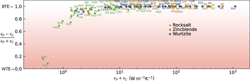
Eq. (1) shows in the first line that the total macroscopic conductivity is determined by two contributions: the particle-like conductivity (), and the wave-like ‘coherence’ conductivity (). In such an equation, the term inside the square brackets is the single-phonon contribution to the total conductivity, , which, as we will show later, is useful for benchmarking fMLPs. The second line shows that originates from phonons that carry heat by propagating particle-like with velocity over lifetime . The term on the third and fourth lines, instead, shows that describes conduction through wave-like tunneling between pairs of phonons at wavevector . It has been shown36, 37 that in simple crystals particle-like propagation dominates over wave-like tunneling (), in complex crystals both these mechanism co-exist (), and in strongly disordered glasses tunneling dominates () 44.
Vibrational and thermal properties from fMLPs
In general, is highly sensitive to both harmonic and anharmonic vibrational properties 46, 47, 48, 37. Therefore, as a first benchmark test for fMLPs, it is natural to compare their predictions for with those obtained from reference first-principles data.
To this end, we begin by calculating the harmonic (, , and ) and third-order anharmonic () vibrational properties that determine . We do this by: (i) relying on the Density-Functional Theory (DFT) data of Refs. 41, 42, calculated using the Perdew, Burke, and Ernzerhof (PBE) functional; or (ii) using SOTA non-proprietary mp-fMLPs trained on DFT-PBE40.
Then, these atomistic vibrational properties are used in Eq. (1)
to calculate the conductivity of the materials in the phononDB-PBE database41, 42 — 103 diverse binary compounds, involving 34 different chemical species and having rocksalt, zincblende, or wurtzite structure.
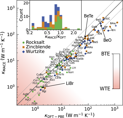
In Fig. 1 we compare the conductivity predicted from first principles (DFT-PBE) or from the mp-fMLP MACE-MP-0 large (trained on PBE) 21, underscoring that predictions are generally compatible within a factor of 2. We also highlight that in about 20% of the compounds studied, the semiclassical particle-like BTE fails to fully describe heat transport and it is crucial to employ the more general WTE. These cases have very low conductivity ( W/mK), which receives significant contributions from both wave-like tunneling (described by the WTE but missing from the BTE) and particle-like propagation (described by both the WTE and BTE) heat-transport mechanism, see Methods Fig. 6.
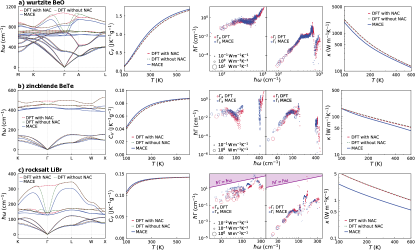
To understand the microscopic origin of the discrepancies in the macroscopic DFT-PBE and MACE-MP-0 conductivities, we select three representative materials — wurtzite BeO, zincblende BeTe, and rocksalt LiBr — and show in Fig. 2 their phonon band structures, specific heat at constant volume, and macroscopic conductivity resolved in terms of contributions from microscopic phonon modes. Examining the phonon band structures in the first column, we observe that MACE-MP-0 tends to underestimate the high-frequency optical vibrational modes compared to DFT-PBE. To further investigate these differences, we plot the DFT-PBE phonons considering or not the non-analytical correction term 49 (NAC). The NAC long-range term is responsible for the energy splitting between the longitudinal-optical and transversal-optical modes in polar dielectrics 49, and is not fully considered in fMLPs trained using a radial cutoff (e.g., for MACE-MP-021 such cutoff is 6 Å, while it is 5 Å for SevenNet22, CHGNet20, and M3GNet19). This explains why the DFT-PBE phonons without NAC are in closer agreement with the MACE-MP-0 phonons. Importantly, it is noticeable that even without NAC, DFT-PBE energies tend to be higher than MACE-MP-0 energies, confirming the general tendency of MACE-MP-0 to underestimate phonon energies 34. Nevertheless, Fig. 2 shows that considering or not the NAC term has a negligible impact on the specific heat at constant volume and on . This can be understood from the third column of Fig. 2, where we show that in these materials a significant amount of heat is carried by low-energy phonons that are negligibly affected by NAC. Specifically, we report the energy-linewidth distributions, resolving the anharmonic and isotopic parts of the linewidths ( and , respectively), and quantifying how much a single phonon mode contributes to the total conductivity with the single-mode contribution to the conductivity , defined in Eq. (1).
The energy-linewidth distributions in Fig. 2a show overall agreement between DFT-PBE and MACE-MP-0 for the phonon modes that are most relevant for conduction, and we see that this implies corresponding macroscopic compatible within . Importantly, Fig. 2b shows that compatibility between predicted from DFT or fMLP can also result from cancellation of errors. E.g., in BeTe there are visible differences in the energy-linewidth distributions, and these largely cancel out when integrated to determine the conductivity. Finally, Fig. 2c illustrates that discrepancies in the energy-linewidth distributions do not always compensate, and can translate into significant differences (a factor of 2) on . We also note that depending on the the chemical composition, the anharmonic linewidths at room temperature can dominate over the isotopic linewidth (e.g., in BeO) or not (e.g., in BeTe), see Methods Table. 2.
The results above motivate us to investigate whether good agreement between DFT and fMLP conductivities is obtained as a result of accurately described microscopic harmonic and anharmonic vibrational properties, or because of compensating errors. To study this, we quantify the discrepancies in the total macroscopic thermal conductivities using the Symmetric Relative Error (SRE),
| (2) |
Next, to quantify the error on the microscopic phonon properties, we introduce the Symmetric Relative Mean Error (SRME) on the single-phonon conductivity:
| (3) |
where
refers to the single-phonon conductivity (term inside square brackets in Eq. (1)) evaluated using DFT, and
refers to the same expression evaluated using fMLP.
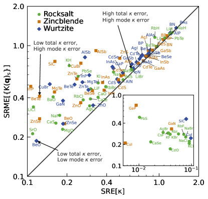
Fig. 3 illustrates that a large SRME generally implies large SRE. Importantly, knowing both SRE and SRME enables us to identify when microscopic error compensation occurs — this is indicated by a large SRME but small SRE.
We note that the SRME[] error can stem from discrepancies in the harmonic (second-order) or anharmonic (third-order) force constants. Therefore, in the Methods (Fig. 7) we discuss how to decompose the SRME and SRE into errors on harmonic and anharmonic vibrational properties.
Accuracy of various SOTA foundation models
Here we utilize the SRE and SMRE descriptors to study the accuracy of different non-proprietary mp-fMLPs on the structures contained in the phononDB-PBE database41, 42, comparing in
Fig. 4 M3GNet19, CHGNet20, MACE-MP-021, and SevenNet22.
To determine if a particular mp-fMLP tends to systematically overestimate or underestimate the conductivity, we rely on the Symmetric Relative Difference (SRD) in the total Wigner conductivity from DFT-PBE or mp-fMLP,
| (4) |
which ranges from -2 to +2, resolving both overestimation and underestimation of the conductivity. Figure 4a summarizes in violin plots the SRD for the compounds in the phononDB-PBE database. Unstable structures with negative phonon frequencies were included considering , i.e., SRD=. This analysis reveals that all the mp-fMLPs assessed in this study tend to underestimate the thermal conductivity. This finding is consistent with the observed systematic underestimation of vibrational frequencies noted in Ref. 34, and might also originate from overestimation of anharmonic linewidths.
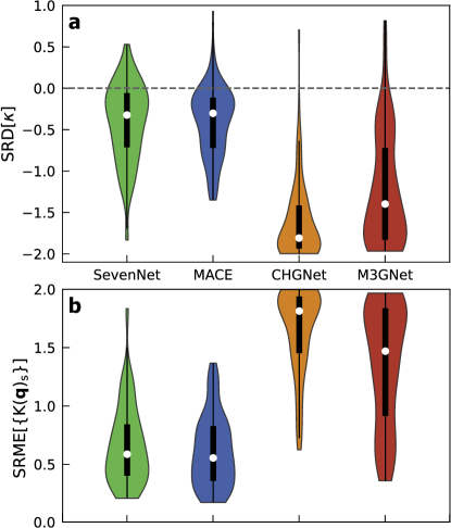
To examine whether the SRD in Fig. 4a is influenced by error compensation, we show in Fig. 4b violin plots for . The most accurate mp-fMLPs, MACE-MP-021, yields zero-shot conductivities compatible within a factor of two of the DFT-PBE values for 69% of the materials in the phononDB-PBE database41, 42.
| 7Net | MACE | CHGNet | M3GNet | |
|---|---|---|---|---|
| mean | ||||
| mean |
Finally, to quantify the overall accuracy of a fMLPs in predicting the macroscopic conductivity over a materials’ database, without resolving the possible compensation of microscopic errors, it is informative to consider the mean of the modulus of the deviations, i.e., the mean of the distribution of SRE (2) — we prefer this over the mean of the SRD distribution, as the latter can be close to zero in the presence of very broad but sign-symmetric distribution.
Importantly, we note that the mean for SRE[] and mean for SRME[] are expected to be comparable in the absence of cancellation of microscopic errors. In contrast, when cancellation of microscopic errors occurs, the mean SRE[] is significantly lower than mean SRME[].
The mean values for SRME[] and SRE[] are reported in Table 1.
Achieving first-principles accuracy via fine-tuning
In the previous section we discussed the ionic conductor LiBr as paradigmatic example where the zero-shot conductivity predictions from MACE-MP-0 are in strong disagreement—about a factor of two—with DFT-PBE reference data.
These conductivity discrepancies might be due to lack of relevant reference data in the MP dataset40 used to train MACE-MP-0, and in this section we introduce a fine-tuning protocol to correct them and achieve first-principles accuracy.
Employing the same DFT settings used to generate reference DFT data (see Methods for details), we prepared three distinct datasets for fine-tuning. Each dataset contains a set of different DFT-PBE frames — with ‘frame’ we mean a set comprising forces, total energy, and stress computed from DFT for a set of atomic positions perturbed from equilibrium. Perturbations consists of rattling (random atomic displacements drawn from Gaussian distribution with standard deviation of 0.03Å)50, and in some cases also a few-percent isotropic rescaling of volume. DFT frames have the same size as those used to compute the reference phononDB-PBE phonons, 4x4x4 supercell of LiBr (512 atoms).
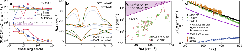
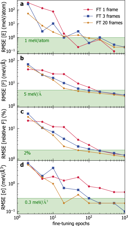
We generated three fine-tuning datasets, containing: (i) one single frame at equilibrium volume and with atomic rattling; (ii) 3 frames, out of which 2 feature ±1% isotropic volume rescaling and rattling, plus the frame in (i) at equilibrium volume and with rattling; (iii) 20 frames, out of which 10 are at equilibrium volume with different rattling, and 10 frames with rattling and volume variations of ±0.25 %, ±0.50%, ±1%, ±2%, and ±5%. Using these datasets, we performed fine-tuning training with number of epochs ranging from 1 to 1000. Fine-tuning MACE yields predictions in closer agreement with the reference DFT-PBE value. Specifically, from Fig. 5a we see that fine-tuning relying on the 3-frame dataset (ii) and for 200 epochs yields compatible within 2% with reference DFT-PBE conductivity. Using the larger fine-tuning dataset (iii) does not show significant improvements, and the single-frame dataset (i) allows to reduce conductivity discrepancies from 47% to 7% in 100 fine-tuning epochs. The excellent agreement between the value of computed from reference DFT-PBE and fine-tuned MACE (3 frames, 200 epochs) originates from low ; this implies also remarkable compatibility for phonons in Fig. 5b, microscopic energy-linewidth distribution in c, and macroscopic in d. It is worth mentioning that conductivity compatibility within 2% corresponds to root-mean-square error (RMSE) on energy <1.0 meV/atom, on forces <5 meV/Å, and on stresses <0.3 meV/Å3; see Methods Fig. 9 for details oh how these errors depend on the fine-tuning dataset’s size, and on the number of fine-tuning training epochs.
Finally, we highlight how the predictions for in the temperature range 100-800 K reproduce experimental measurements51, in both trend and magnitude (error bars show the compatibility threshold of 20% discussed in Ref. 51).
We also emphasize that employing the WTE is essential for accurately describing heat transport in LiBr at high temperatures.
In fact, upon increasing temperature the tunneling conductivity becomes more important and non-negligible compared to the propagation conductivity , and the total WTE conductivity is in better agreement with the experimental trend compared to the BTE (propagation-only) conductivity .
Finally, at 300 K our is compatible also with predictions from ab-initio (PBE) molecular dynamics (aiMD)47.
Conclusions
We introduced a framework that leverages foundation models for atomistic materials chemistry19, 20, 21, 22, 23, 24, 25, 26, 27, 28, 29, 30, 31 and the Wigner formulation of heat transport36, 37 to address the major challenges of current techniques for designing heat-management materials: high computational cost, limited transferability, or lack of physics awareness.
In particular, we demonstrated that our framework can systematically achieve quantum accuracy in thermal conductivity predictions at computational costs that are orders of magnitude lower than current methods, which rely on density-functional theory for direct evaluations or for full training of conventional (not fully composition-transferable) machine-learning potentials.
Importantly, our physics-aware framework also overcomes the reliability issues (unknown unknowns) of current end-to-end machine-learning methods for predicting vibrational or thermal properties.
We developed benchmark tests based on technologically relevant observables, such as thermal conductivity, and showed applications to a database41, 42 of chemically and structurally diverse materials using state-of-the-art foundation models (SevenNet22, MACE-MP-021, CHGNet20, and M3GNet19).
Finally, we have shown that our framework enables the screening or prediction of materials that violate semiclassical Boltzmann transport, which are crucial for applications ranging from thermal insulation11, 37 to neuromorphic computing12.
Ultimately, our framework paves the way for the theory-driven optimization, design, and discovery of materials for next-generation energy and information-management technologies.
Methods
Vibrational properties relevant to compute
In this section we discuss the relation between interatomic vibrational energies and the quantities that appear in the WTE thermal conductivity expression (1).
The starting point is the Born-Oppenheimer Hamiltonian for atomic vibrations 37 expanded up to anharmonic third order in the atomic displacements from equilibrium, and accounting for energy perturbations due to presence of isotopes 52,
| (5) |
Here, and are the momentum and position-displacement operators for the atom having isotope-averaged mass , position ( is the Bravais-lattice vector and the position in the crystal’s unit cell), and along the Cartesian direction ; the last term describes kinetic-energy perturbations induced by isotopes ( is the exact mass of atom at , we adopt the common approximation52, 53 that the mass depends only on the index and not on the lattice vector ). The leading (harmonic) term in Eq. (5) determines the vibrational frequencies. In particular, the Fourier transform of the mass-rescaled Hessian of the interatomic potential yields the dynamical matrix at wavevector ,
| (6) |
and by diagonalizing the dynamical matrix,
| (7) |
one obtains from the eigenvalues the phonon energies of the solid ( is a band index ranging from 1 to 3, where is the number of atoms in the unit cell), and from the eigenvectors the displacement patterns of atom in direction for the phonon having wavevector and mode .
As discusses in detail in Ref. 37, the velocity operator appearing in the WTE conductivity expression (1) is determined by the wavevector derivative of the square root of the dynamical matrix:
| (8) |
The anharmonic linewidths , which contribute to the total linewidths appearing in Eq. (1), are the energy broadenings due to anharmonic three-phonon interactions 53, 54, 55, 56, 57. It can be shown58, that these are determined by the third derivative in Eq. (5). In formulas, the anharmonic linewidth of the phonon is
| (9) |
where is the Bose-Einstein distribution, is the Kronecker delta (equal to 1 if is a reciprocal lattice vector, 0 otherwise), is the Dirac delta. The linewidth due to isotopic-mass disorder is determined exclusively by harmonic properties and concentration of isotopes52:
| (10) |
where describes the variance of the isotopic masses of atom ( and are the mole fraction and mass, respectively, of the th isotope of atom ; is the weighted average mass).
Failures of semiclassical Boltzmann transport
As anticipated in the main text, our automated framework can be used to identify materials in which the semiclassical particle-like BTE fails. This happens when particle-like propagation mechanisms — described by both the BTE and WTE36, 43, 59, and determining in Eq. (1) — do not dominate over wave-like tunneling mechanisms — missing from the BTE but described by the WTE and determining in Eq. (1).
Failures of the BTE have been discussed to appear in, e.g., strongly anharmonic complex crystals for energy harvesting60, 61, 62, 63, 64, 65, 66, 67, 68, 69, 70, 71, 72, thermal barrier coatings 73, 74, 75, 45, as well as in several disordered functional materials 76, 77, 78, 79, 80, 81.
Our automated framework computes the total Wigner thermal conductivity 37, and therefore can be used to find materials that violate semiclassical Boltzmann thermal transport.
In Fig. 6 we show that among the 103 compounds analyzed at 300 K, the BTE fails in materials with low thermal conductivity ( W/mK), such as AgBr and AgCl, since the wave-like tunneling conductivity becomes comparable to the particle-like propagation conductivity. We also note that in simple crystals with large conductivity, the BTE is accurate as the particle-like propagation conductivity dominates over the wave-like tunneling conductivity.
Symmetric Relative Mean Error on harmonic and anharmonic vibrational properties. The analyses reported in the main text discuss SRME as a descriptor that is informative of the accuracy of fMLPs in describing microscopic harmonic and anharmonic properties. In this section we provide the tools to resolve whether a large SRME originates from large errors in microscopic harmonic properties, or large errors in anharmonic properties, or from both. To this aim, we employ the expression for the microscopic, single-phonon contributions to the thermal conductivity (see terms inside the square brackets in Eq. (1)) to define descriptors that quantity the accuracy with which harmonic and anharmonic properties are predicted. In particular, we note that the conductivity contribution of a phonon is a function of: (i) all the phonon frequencies at a fixed wavevector and variable mode ( is the number of phonon bands, equal to 3 times the number of atoms in the crystal’s unit cell 82); (ii) all velocity-operator elements at fixed , and variable ; (iii) all isotopic linewidths at fixed and variable , , which depend solely on harmonic properties, see Eq. 10; (iv) the anharmonic linewidths at fixed and variable . This can be summarized using the following notation: where the curly brackets denote the set of values of a certain quantity over all the bands at fixed (e.g., ).
To quantify the impact of errors on the harmonic (har) and anharmonic (anh) properties on the single-phonon conductivity contributions, we define the Symmetric Relative Mean Error (SRME) on these properties as follows:
| (11) |
| (12) |
where we have used the shorthand notation . Intuitively, SRME[har] (11) is large when harmonic vibrational properties (, or , or ) differ between DFT and fMLP, while SRME[anh] (12) is large when the anharmonic linewidths () differ between DFT and fMLP. We show in Fig. 7 that small SRME[har] and small SRME[anh] (e.g., as in BeO), imply a small SRE[]
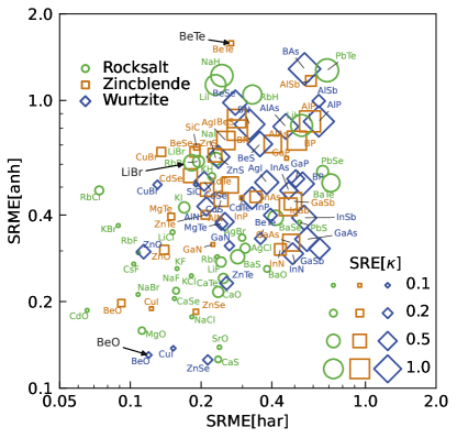
Fig. 7 also shows that often large SRME[har] and large SRME[anh] (e.g. LiBr) translate into large ; however there also cases (e.g. BeTe) in which large SRME[har] and large SRME[anh] can also compensate each other and result in a small . This confirms the statements made in the main text on not being a reliable descriptor for the capability of fMLPs to capture the harmonic and anharmonic physics underlying heat conduction. In contrast, having both small SRME[har] and small SRME[anh] is a sufficient condition to accurately capture harmonic and anharmonic vibrational properties, as well as thermal conductivity.
Overall, these tests illustrate the importance of benchmarking the accuracy of fMLPs in predicting both microscopic harmonic and anharmonic vibrational properties, further motivating the introduction of the SRME[].
Influence of isotopic scattering on conductivity. To analyze the influence of isotope scattering on the conductivity, we compare thermal conductivity values with and without considering the linewidths from isotope mass-disorder (Eq. (10)). The results are summarized in Table 2. In wurtzite BeO and rocksalt LiBr, the impact of isotope scattering is minimal or small, respectively. However, in zincblende BeTe, as shown in Fig. 2b, isotopic and anharmonic linewidths have comparable values, both affecting the thermal conductivity. In this material, MACE-MP-0 significantly overestimates some linewidths compared to DFT-PBE, and this compensates for the overestimation in other regions. Consequently, MACE-MP-0 shows a significantly larger error in thermal conductivity when isotope scattering is not considered.
| wurtzite BeO | zincblende BeTe | rocksalt LiBr | ||||
|---|---|---|---|---|---|---|
| DFT | MACE | DFT | MACE | DFT | MACE | |
| with | 286.391 | 259.443 | 78.246 | 69.138 | 1.789 | 0.948 |
| without | 291.963 | 263.956 | 289.374 | 402.030 | 1.803 | 0.951 |
Automated Wigner Conductivity Workflow.
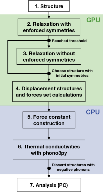
The workflow, outlined in Fig. 8, includes structure relaxation, force constant computation, thermal conductivity evaluation and analysis. To automate the calculation of interatomic forces, we developed an interface between the packages ase83 (version 3.23.0) and phono3py41, 84 (version 3.2.0). Atomic positions and cell parameters were simultaneously relaxed to minimize stresses and ensure positive phonon frequencies. Since the determination of irreducible points during thermal conductivity calculations depends on the crystal symmetry, it is essential to consider symmetries. During the initial relaxation stage, symmetries are explicitly enforced as constraints while simultaneously relaxing atomic positions and cell parameters. After each step of atomic position relaxation, cell parameters are adjusted if the total forces exceed a a certain threshold (values are fMLP-specific and discussed later). In the second stage, the symmetry constraint is removed to allow for finer atomic adjustments and a complete relaxation of the structure. The joint relaxation of atomic positions and cell parameters is applied once more. If the symmetry is preserved, the final relaxed structure is used. If symmetry is broken, the structure from the first stage, with enforced symmetry, is retained. Finally, an additional relaxation of atomic positions with fixed cell parameters is performed using a stricter threshold to ensure the structure reaches a stable energy minimum at a fixed volume for accurate phonon calculations.
To ensure positive phonons, strict thresholds were established, tailored to each individual model. M3GNet required thresholds of eV/Å and eV/Å. For CHGNet, MACE-MP-0, and SevenNet, the thresholds were set to eV/Å and eV/Å for initial and final values, respectively. In the supercell force-constant calculations, we used the same parameters used in the DFT reference data41, 42.
Thermal conductivities were computed using phono3py following Ref. 41, 84. A -mesh was used for rocksalt and zincblende structures, and a -mesh for wurtzite structures. The collision operator was computed using the tetrahedron method. For Fig. 2, linewidths were calculated on a -mesh, for graphical clarity. We utilized version 3 of phono3py for anharmonic linewidth calculations and employed the Wang method 85, 86 for the NAC term, as implemented in the phonopy84, 87 package (version 2.26.6). When structures with negative phonon frequencies were found with mp-fMLPs, these were discarded from subsequent thermal-conductivity analysis.
DFT and zero-shot mp-fMLP calculations. Computational details of the DFT calculations underlying the phononDB-PBE database can be found in Refs. 41, 42. These employed the Perdew, Burke, and Ernzerhof (PBE) exchange-correlation functional 88, consistent with the approach used for generating the MP dataset 40, used to train mp-fMLPs.
We note that the DFT parameters used to generate the phononDB-PBE database are similar but not always exactly equal to those used for DFT calculations in the MP database. In the regime of computational convergence, variations of the DFT parameters at fixed functional are supposed to yield unimportant effects on the thermal conductivity. In particular, Ref. 89 shows that for the prototypical case of silicon, computing the force constants using DFT parameters within the range of ‘computationally converged values’ found in the literature produces conductivity variations that are within 7 , and also shows that in ideal cases varying DFT parameters within the domain of computational convergence should yield conductivity variations smaller than 2 . As such, the significant discrepancies shown in Fig. 3 are expected to be not caused by possible small differences in the DFT parameters.
The computational details on the mp-fMLPs can be found in the following references: M3GNet19, CHGNet20, MACE-MP-021, and SevenNet22. M3GNet was used through the matgl90 (version 1.1.2) package with the M3GNet-MP-2021.2.8-PES model. The CHGNet version 0.3.8 was used. The MACE-MP-0 2024-01-07-mace-128-L2 model was run through LAMMPS91. SevenNet was used through the sevenn package (version 0.9.2) with the SevenNet-0_11July2024 model. The details on the violin plots presented in Fig. 4 can be found in Ref. 92.
Details on fine-tuning. In this section we discuss how the size of the fine-tuning dataset and the number of fine-tuning epochs influence the accuracy with which energies, forces, and stresses are described. Results for LiBr are shown in Fig. 9; we underscore that to achieve 2% accuracy on the conductivity it is necessary to have RMSE on energy smaller than 1.0 meV/atom, RMSE on forces smaller than 5 meV/Å (about 2% relative error), and RMSE on stresses smaller than 0.3 meV/Å3.
The three DFT datasets used for fine-tuning are made up of DFT calculations in 4x4x4 supercells of LiBr (same size used for the phonon calculation in the phononDB-PBE42, 41 database) perturbed from equilibrium with atomic rattling and in some cases also volume variations from 0.25% to 5%.
All DFT calculations are performed employing the Perdew, Burke, and Ernzerhof (PBE) exchange-correlation functional 88, and the projector augmented wave (PAW) formalism for electronic minimization, implemented within the VASP (Vienna ab initio simulation package) code 93, 94.
Following Ref. 42, we use a 600 eV plane-wave-basis cutoff (20% higher than the default one), and the Brillouin zone is sampled at the Gamma point.
Using these DFT settings, the LiBr structure in the phononDB-PBE database shows a residual negative stress of 960 Bar. Therefore, to make the most accurate possible comparison between fine-tuned MACE-MP-0 and reference DFT data, we relaxed the fine-tuned MACE-MP-0 structure exactly to the same residual stress present in the reference DFT-PBE data.
The MACE-MP-0 2024-01-07-mace-128-L2 model https://github.com/ACEsuit/mace-mp/commits/mace_mp_0 was fine-tuned using the mace_run_train script in the main branch of https://github.com/ACEsuit/mace.
The training started from the last checkpoint of MACE-MP-0 L2. The three datasets discussed above were used to perform three independent trainings.
For trainings on the 1-frame and 3-frame datasets we employed a batch size of 1, and for trainings on the 20-frame dataset we used a batch of size 4.
Since our fine-tuning datasets were computed with the DFT-PBE functional, which was also employed to generate the MP database40 used to train MACE-MP-0, in the fine-tuning we kept the E0s fixed at their original MACE-MP-0 value.
Representative examples of training scripts are available at: https://github.com/MSimoncelli/fMLP_conductivity.git. The fine-tuning was performed on Nvidia Tesla A100 SXM4 80GB GPU.
Computational cost.
The SevenNet, MACE, and CHGNet calculations were performed on an Nvidia Tesla A100 SXM4 80GB GPU, with the relaxation and force calculations for all 103 structures costing approximately GPU hours per model. M3GNet was executed on AMD EPYC 7702 CPUs, with relaxation and force calculations costing around CPU hours. Thermal conductivity calculations for all 103 structures required about CPU hours per model, and similar resources were needed for evaluating thermal conductivity from the DFT force constants. Overall, the analysis of these four models required approximately GPU hours and CPU hours.
Data availability.
The phononDB-PBE dataset including the displacements generated by phono3py and the corresponding force sets are available https://github.com/atztogo/phonondb 41, 42. The remaining dataset will be made available in the future.
Code availability.
The phono3py and phonopy packages are available at https://github.com/phonopy/; the ase package is available at https://gitlab.com/ase/ase. matgl containing the M3GNet model is available at https://github.com/materialsvirtuallab/matgl; the CHGNet model and package is available at https://github.com/CederGroupHub/chgnet; the SevenNet model and package is available at https://github.com/MDIL-SNU/SevenNet. The MACE used through LAMMPS91 is available at https://github.com/ACEsuit/lammps, and the MACE-MP-0 model is available at https://github.com/ACEsuit/mace-mp. The Hiphive package is available at https://gitlab.com/materials-modeling/hiphive.
Acknowledgements
The computational resources were provided by: (i) the Kelvin2 HPC platform at the NI-HPC Centre (funded by EPSRC and jointly managed by Queen’s University Belfast and Ulster University); (ii) the UK National Supercomputing Service ARCHER2, for which access was obtained via the UKCP consortium and funded by EPSRC [EP/X035891/1].
M. S. acknowledges support from Gonville and Caius College. P.A. acknowledges support from SNSF through Post.Doc mobility fellowship P500PN_206693.
We thank William C. Witt and Ilyes Batatia for the useful discussions, and we gratefully acknowledge Atsushi Togo for having provided harmonic and anharmonic force constants computed using density functional theory (PBE functional) from the phononDB-PBE database 41, 42.
Author contributions
M.S. conceived and supervised the project. B.P. developed the automated computational framework and performed the numerical calculations with inputs from P.A., G.C., and M.S. The results were analyzed and organized by B.P. and M.S., with inputs from P.A. All authors contributed to discussing the results, writing and editing the manuscript.
Competing interests
CG has equity interest of Symmetric Group LLP that licenses force fields commercially and also in Ångstrom AI. The other authors declare that they have no competing interest.
Additional information
Correspondence and requests for materials should be addressed to Michele Simoncelli.
References
- Blank et al. [1995] T. B. Blank, S. D. Brown, A. W. Calhoun, and D. J. Doren, The Journal of Chemical Physics 103, 4129 (1995).
- Behler and Parrinello [2007] J. Behler and M. Parrinello, Physical Review Letters 98, 146401 (2007), publisher: American Physical Society.
- Bartók et al. [2010] A. P. Bartók, M. C. Payne, R. Kondor, and G. Csányi, Physical Review Letters 104, 136403 (2010).
- Rupp et al. [2012] M. Rupp, A. Tkatchenko, K.-R. Müller, and O. A. von Lilienfeld, Physical Review Letters 108, 058301 (2012), publisher: American Physical Society.
- Zhang et al. [2018] L. Zhang, J. Han, H. Wang, R. Car, and W. E, Physical Review Letters 120, 143001 (2018).
- Drautz [2019] R. Drautz, Physical Review B 99, 014104 (2019), publisher: American Physical Society.
- Seko et al. [2019] A. Seko, A. Togo, and I. Tanaka, Physical Review B 99, 214108 (2019).
- Deringer et al. [2021] V. L. Deringer, A. P. Bartók, N. Bernstein, D. M. Wilkins, M. Ceriotti, and G. Csányi, Chemical Reviews 121, 10073 (2021).
- Batzner et al. [2022] S. Batzner, A. Musaelian, L. Sun, M. Geiger, J. P. Mailoa, M. Kornbluth, N. Molinari, T. E. Smidt, and B. Kozinsky, Nature Communications 13, 2453 (2022), publisher: Nature Publishing Group.
- Kocer et al. [2022] E. Kocer, T. W. Ko, and J. Behler, Annual Review of Physical Chemistry 73, 163 (2022).
- Qian et al. [2021] X. Qian, J. Zhou, and G. Chen, Nature Materials 20, 1188 (2021), number: 9 Publisher: Nature Publishing Group.
- Nataf et al. [2024] G. F. Nataf, S. Volz, J. Ordonez-Miranda, J. Íñiguez González, R. Rurali, and B. Dkhil, Nature Reviews Materials , 1 (2024).
- Okabe et al. [2024] R. Okabe, A. Chotrattanapituk, A. Boonkird, N. Andrejevic, X. Fu, T. S. Jaakkola, Q. Song, T. Nguyen, N. Drucker, S. Mu, Y. Wang, B. Liao, Y. Cheng, and M. Li, Nature Computational Science 10.1038/s43588-024-00661-0 (2024).
- Ojih et al. [2024] J. Ojih, M. Al-Fahdi, Y. Yao, J. Hu, and M. Hu, Journal of Materials Chemistry A 12, 8502 (2024).
- Rodriguez et al. [2023] A. Rodriguez, C. Lin, H. Yang, M. Al-Fahdi, C. Shen, K. Choudhary, Y. Zhao, J. Hu, B. Cao, H. Zhang, et al., npj Computational Materials 9, 20 (2023).
- Rose et al. [2023] V. D. Rose, A. Kozachinskiy, C. Rojas, M. Petrache, and P. Barceló, Three iterations of $(d-1)$-WL test distinguish non isometric clouds of $d$-dimensional points (2023), arXiv:2303.12853 [cs].
- Gilmer et al. [2017] J. Gilmer, S. S. Schoenholz, P. F. Riley, O. Vinyals, and G. E. Dahl, in Proceedings of the 34th International Conference on Machine Learning (PMLR, 2017) pp. 1263–1272, iSSN: 2640-3498.
- Batatia et al. [2023] I. Batatia, D. P. Kovács, G. N. C. Simm, C. Ortner, and G. Csányi, MACE: Higher Order Equivariant Message Passing Neural Networks for Fast and Accurate Force Fields (2023), arXiv:2206.07697 [cond-mat, physics:physics, stat].
- Chen and Ong [2022] C. Chen and S. P. Ong, Nature Computational Science 2, 718 (2022), publisher: Nature Publishing Group.
- Deng et al. [2023] B. Deng, P. Zhong, K. Jun, J. Riebesell, K. Han, C. J. Bartel, and G. Ceder, Nature Machine Intelligence 5, 1031 (2023), publisher: Nature Publishing Group.
- Batatia et al. [2024] I. Batatia, P. Benner, Y. Chiang, A. M. Elena, D. P. Kovács, J. Riebesell, X. R. Advincula, M. Asta, M. Avaylon, W. J. Baldwin, F. Berger, N. Bernstein, A. Bhowmik, S. M. Blau, V. Cărare, J. P. Darby, S. De, F. Della Pia, V. L. Deringer, R. Elijošius, Z. El-Machachi, F. Falcioni, E. Fako, A. C. Ferrari, A. Genreith-Schriever, J. George, R. E. A. Goodall, C. P. Grey, P. Grigorev, S. Han, W. Handley, H. H. Heenen, K. Hermansson, C. Holm, J. Jaafar, S. Hofmann, K. S. Jakob, H. Jung, V. Kapil, A. D. Kaplan, N. Karimitari, J. R. Kermode, N. Kroupa, J. Kullgren, M. C. Kuner, D. Kuryla, G. Liepuoniute, J. T. Margraf, I.-B. Magdău, A. Michaelides, J. H. Moore, A. A. Naik, S. P. Niblett, S. W. Norwood, N. O’Neill, C. Ortner, K. A. Persson, K. Reuter, A. S. Rosen, L. L. Schaaf, C. Schran, B. X. Shi, E. Sivonxay, T. K. Stenczel, V. Svahn, C. Sutton, T. D. Swinburne, J. Tilly, C. van der Oord, E. Varga-Umbrich, T. Vegge, M. Vondrák, Y. Wang, W. C. Witt, F. Zills, and G. Csányi, A foundation model for atomistic materials chemistry (2024), arXiv:2401.00096 [cond-mat, physics:physics].
- Park et al. [2024] Y. Park, J. Kim, S. Hwang, and S. Han, Journal of Chemical Theory and Computation 20, 4857 (2024), publisher: American Chemical Society.
- Yang et al. [2024] H. Yang, C. Hu, Y. Zhou, X. Liu, Y. Shi, J. Li, G. Li, Z. Chen, S. Chen, C. Zeni, M. Horton, R. Pinsler, A. Fowler, D. Zügner, T. Xie, J. Smith, L. Sun, Q. Wang, L. Kong, C. Liu, H. Hao, and Z. Lu, Mattersim: A deep learning atomistic model across elements, temperatures and pressures (2024), arXiv:2405.04967 [cond-mat.mtrl-sci] .
- Merchant et al. [2023] A. Merchant, S. Batzner, S. S. Schoenholz, M. Aykol, G. Cheon, and E. D. Cubuk, Nature 624, 80 (2023), publisher: Nature Publishing Group.
- Choudhary and DeCost [2021] K. Choudhary and B. DeCost, npj Computational Materials 7, 185 (2021).
- Chen et al. [2019] C. Chen, W. Ye, Y. Zuo, C. Zheng, and S. P. Ong, Chemistry of Materials 31, 3564 (2019).
- Ward et al. [2017] L. Ward, R. Liu, A. Krishna, V. I. Hegde, A. Agrawal, A. Choudhary, and C. Wolverton, Physical Review B 96, 024104 (2017).
- Zuo et al. [2021] Y. Zuo, M. Qin, C. Chen, W. Ye, X. Li, J. Luo, and S. P. Ong, Materials Today 51, 126 (2021).
- Xie and Grossman [2018] T. Xie and J. C. Grossman, Physical Review Letters 120, 145301 (2018).
- Gibson et al. [2022] J. Gibson, A. Hire, and R. G. Hennig, npj Computational Materials 8, 211 (2022).
- Goodall et al. [2022] R. E. A. Goodall, A. S. Parackal, F. A. Faber, R. Armiento, and A. A. Lee, Science Advances 8, eabn4117 (2022).
- Riebesell et al. [2024] J. Riebesell, R. E. A. Goodall, P. Benner, Y. Chiang, B. Deng, A. A. Lee, A. Jain, and K. A. Persson, Matbench Discovery – A framework to evaluate machine learning crystal stability predictions (2024), arXiv:2308.14920 [cond-mat].
- Yu et al. [2024] H. Yu, M. Giantomassi, G. Materzanini, J. Wang, and G.-M. Rignanese, Systematic assessment of various universal machine-learning interatomic potentials (2024), arXiv:2403.05729 [cond-mat].
- Deng et al. [2024] B. Deng, Y. Choi, P. Zhong, J. Riebesell, Z. Li, K. Jun, K. A. Persson, and G. Ceder, Overcoming systematic softening in universal machine learning interatomic potentials by fine-tuning (2024), arXiv:2405.07105.
- Lee et al. [2024] H. Lee, V. I. Hegde, C. Wolverton, and Y. Xia, Accelerating High-Throughput Phonon Calculations via Machine Learning Universal Potentials (2024), arXiv:2407.09674 [cond-mat].
- Simoncelli et al. [2019] M. Simoncelli, N. Marzari, and F. Mauri, Nature Physics 15, 809 (2019).
- Simoncelli et al. [2022] M. Simoncelli, N. Marzari, and F. Mauri, Physical Review X 12, 041011 (2022).
- Peierls [1929] R. Peierls, Annalen der Physik 395, 1055 (1929).
- Allen and Feldman [1989] P. B. Allen and J. L. Feldman, Physical Review Letters 62, 645 (1989).
- Jain et al. [2013] A. Jain, S. P. Ong, G. Hautier, W. Chen, W. D. Richards, S. Dacek, S. Cholia, D. Gunter, D. Skinner, G. Ceder, and K. A. Persson, APL Materials 1, 011002 (2013).
- Togo et al. [2015] A. Togo, L. Chaput, and I. Tanaka, Phys. Rev. B 91, 094306 (2015).
- Seko et al. [2015] A. Seko, A. Togo, H. Hayashi, K. Tsuda, L. Chaput, and I. Tanaka, Physical Review Letters 115, 205901 (2015).
- Simoncelli et al. [2020] M. Simoncelli, N. Marzari, and A. Cepellotti, Phys. Rev. X 10, 011019 (2020).
- Simoncelli et al. [2023] M. Simoncelli, F. Mauri, and N. Marzari, npj Computational Materials 9, 1 (2023).
- Pazhedath et al. [2024] A. Pazhedath, L. Bastonero, N. Marzari, and M. Simoncelli, Phys. Rev. Appl. 22, 024064 (2024).
- Plata et al. [2017] J. J. Plata, P. Nath, D. Usanmaz, J. Carrete, C. Toher, M. de Jong, M. Asta, M. Fornari, M. B. Nardelli, and S. Curtarolo, npj Computational Materials 3, 1 (2017), publisher: Nature Publishing Group.
- Knoop et al. [2023] F. Knoop, T. A. Purcell, M. Scheffler, and C. Carbogno, Physical Review Letters 130, 236301 (2023).
- Bandi et al. [2024] S. Bandi, C. Jiang, and C. A. Marianetti, Machine Learning: Science and Technology (2024).
- Gonze and Lee [1997a] X. Gonze and C. Lee, Physical Review B 55, 10355 (1997a).
- Eriksson et al. [2019] F. Eriksson, E. Fransson, and P. Erhart, Advanced Theory and Simulations 2, 1800184 (2019).
- Hakansson and Ross [1989] B. Hakansson and R. G. Ross, Journal of Physics: Condensed Matter 1, 3977 (1989).
- Tamura [1983] S.-i. Tamura, Phys. Rev. B 27, 858 (1983).
- Fugallo et al. [2013] G. Fugallo, M. Lazzeri, L. Paulatto, and F. Mauri, Phys. Rev. B 88, 045430 (2013).
- Togo and Seko [2024] A. Togo and A. Seko, The Journal of Chemical Physics 160, 211001 (2024).
- Tadano et al. [2014] T. Tadano, Y. Gohda, and S. Tsuneyuki, Journal of Physics: Condensed Matter 26, 225402 (2014).
- Carrete et al. [2017] J. Carrete, B. Vermeersch, A. Katre, A. van Roekeghem, T. Wang, G. K. Madsen, and N. Mingo, Comput. Phys. Commun. 220, 351 (2017).
- Li et al. [2014] W. Li, J. Carrete, N. A. Katcho, and N. Mingo, Computer Physics Communications 185, 1747 (2014).
- Paulatto et al. [2013] L. Paulatto, F. Mauri, and M. Lazzeri, Physical Review B 87, 214303 (2013).
- Dragašević and Simoncelli [2023] J. Dragašević and M. Simoncelli, arXiv:2303.12777 (2023).
- Di Lucente et al. [2023] E. Di Lucente, M. Simoncelli, and N. Marzari, Physical Review Research 5, 033125 (2023).
- Jain [2020] A. Jain, Phys. Rev. B 102, 201201 (2020).
- Xia et al. [2020] Y. Xia, V. I. Hegde, K. Pal, X. Hua, D. Gaines, S. Patel, J. He, M. Aykol, and C. Wolverton, Phys. Rev. X 10, 041029 (2020).
- Shen et al. [2024] X. Shen, N. Ouyang, Y. Huang, Y.-H. Tung, C.-C. Yang, M. Faizan, N. Perez, R. He, A. Sotnikov, K. Willa, C. Wang, Y. Chen, and E. Guilmeau, Advanced Science 11, 2400258 (2024).
- Pandey et al. [2022] T. Pandey, M.-H. Du, D. S. Parker, and L. Lindsay, Materials Today Physics 28, 100881 (2022).
- Fiorentino and Baroni [2023] A. Fiorentino and S. Baroni, Physical Review B 107, 054311 (2023).
- Zhou et al. [2024] S. Zhou, E. Xiao, H. Ma, K. Gofryk, C. Jiang, M. E. Manley, D. H. Hurley, and C. A. Marianetti, Physical Review Letters 132, 106502 (2024).
- Zheng et al. [2024] J. Zheng, C. Lin, C. Lin, G. Hautier, R. Guo, and B. Huang, npj Computational Materials 10, 1 (2024), publisher: Nature Publishing Group.
- Jia et al. [2023] F. Jia, S. Zhao, J. Wu, L. Chen, T.-H. Liu, and L.-M. Wu, Angewandte Chemie 135, e202315642 (2023).
- Tadano and Saidi [2022] T. Tadano and W. A. Saidi, Physical Review Letters 129, 185901 (2022).
- Bernges et al. [2022] T. Bernges, R. Hanus, B. Wankmiller, K. Imasato, S. Lin, M. Ghidiu, M. Gerlitz, M. Peterlechner, S. Graham, G. Hautier, Y. Pei, M. R. Hansen, G. Wilde, G. J. Snyder, J. George, M. T. Agne, and W. G. Zeier, Advanced Energy Materials 12, 2200717 (2022).
- Yang et al. [2022] X. Yang, J. Tiwari, and T. Feng, Materials Today Physics 24, 100689 (2022).
- Zeng et al. [2024] Z. Zeng, X. Shen, R. Cheng, O. Perez, N. Ouyang, Z. Fan, P. Lemoine, B. Raveau, E. Guilmeau, and Y. Chen, Nature Communications 15, 3007 (2024), publisher: Nature Publishing Group.
- Caldarelli et al. [2022] G. Caldarelli, M. Simoncelli, N. Marzari, F. Mauri, and L. Benfatto, Physical Review B 106, 024312 (2022).
- Xia et al. [2023] Y. Xia, D. Gaines, J. He, K. Pal, Z. Li, M. G. Kanatzidis, V. Ozoliņš, and C. Wolverton, Proceedings of the National Academy of Sciences 120, e2302541120 (2023).
- Luo et al. [2020] Y. Luo, X. Yang, T. Feng, J. Wang, and X. Ruan, Nature Communications 11, 2554 (2020).
- Harper et al. [2024] A. F. Harper, K. Iwanowski, W. C. Witt, M. C. Payne, and M. Simoncelli, Physical Review Materials 8, 043601 (2024), publisher: American Physical Society.
- Liu et al. [2023] Y. Liu, H. Liang, L. Yang, G. Yang, H. Yang, S. Song, Z. Mei, G. Csányi, and B. Cao, Advanced Materials 35, 2210873 (2023).
- Ndour et al. [2023] M. Ndour, P. Jund, and L. Chaput, Journal of Non-Crystalline Solids 621, 122618 (2023).
- Lundgren et al. [2021] N. W. Lundgren, G. Barbalinardo, and D. Donadio, Phys. Rev. B 103, 024204 (2021).
- Kielar et al. [2024] S. Kielar, C. Li, H. Huang, R. Hu, C. Slebodnick, A. Alatas, and Z. Tian, Nature Communications 15, 6981 (2024), publisher: Nature Publishing Group.
- Simoncelli et al. [2024] M. Simoncelli, D. Fournier, M. Marangolo, E. Balan, K. Béneut, B. Baptiste, B. Doisneau, N. Marzari, and F. Mauri, Temperature-invariant heat conductivity from compensating crystalline and glassy transport: from the Steinbach meteorite to furnace bricks (2024), arXiv:2405.13161 [cond-mat].
- Ziman [1960] J. M. Ziman, Electrons and phonons: the theory of transport phenomena in solids (Oxford university press, 1960).
- Larsen et al. [2017] A. H. Larsen, J. J. Mortensen, J. Blomqvist, I. E. Castelli, R. Christensen, M. Dułak, J. Friis, M. N. Groves, B. Hammer, C. Hargus, E. D. Hermes, P. C. Jennings, P. B. Jensen, J. Kermode, J. R. Kitchin, E. L. Kolsbjerg, J. Kubal, K. Kaasbjerg, S. Lysgaard, J. B. Maronsson, T. Maxson, T. Olsen, L. Pastewka, A. Peterson, C. Rostgaard, J. Schiøtz, O. Schütt, M. Strange, K. S. Thygesen, T. Vegge, L. Vilhelmsen, M. Walter, Z. Zeng, and K. W. Jacobsen, Journal of Physics: Condensed Matter 29, 273002 (2017).
- Togo et al. [2023] A. Togo, L. Chaput, T. Tadano, and I. Tanaka, Journal of Physics: Condensed Matter 35, 353001 (2023), publisher: IOP Publishing.
- Wang et al. [2010] Y. Wang, J. J. Wang, W. Y. Wang, Z. G. Mei, S. L. Shang, L. Q. Chen, and Z. K. Liu, Journal of Physics: Condensed Matter 22, 202201 (2010).
- Gonze and Lee [1997b] X. Gonze and C. Lee, Physical Review B 55, 10355 (1997b).
- Togo [2023] A. Togo, Journal of the Physical Society of Japan 92, 012001 (2023).
- Perdew et al. [1996] J. P. Perdew, K. Burke, and M. Ernzerhof, Physical Review Letters 77, 3865 (1996).
- Jain and McGaughey [2015] A. Jain and A. J. McGaughey, Computational Materials Science 110, 115 (2015).
- Ko et al. [2023] T. W. Ko, M. Nassar, S. Miret, E. Liu, and S. P. Ong, Materials graph library (2023).
- Plimpton [1995] S. Plimpton, Journal of Computational Physics 117, 1 (1995).
- Hintze and Nelson [1998] J. L. Hintze and R. D. Nelson, The American Statistician 52, 181 (1998).
- Kresse and Hafner [1993] G. Kresse and J. Hafner, Physical Review B 47, 558 (1993).
- Kresse and Furthmüller [1996] G. Kresse and J. Furthmüller, Computational Materials Science 6, 15 (1996).