An Empirical Analysis of Compute-Optimal Inference for Problem-Solving with Language Models

Abstract

The optimal training configurations of large language models (LLMs) with respect to model sizes and compute budgets have been extensively studied. But how to optimally configure LLMs during inference has not been explored in sufficient depth. We study compute-optimal inference: designing models and inference strategies that optimally trade off additional inference-time compute for improved performance. As a first step towards understanding and designing compute-optimal inference methods, we assessed the effectiveness and computational efficiency of multiple inference strategies such as Greedy Search, Majority Voting, Best-of-N, Weighted Voting, and their variants on two different Tree Search algorithms, involving different model sizes and computational budgets. We found that a smaller language model with a novel tree search algorithm typically achieves a Pareto-optimal trade-off. These results highlight the potential benefits of deploying smaller models equipped with more sophisticated decoding algorithms in budget-constrained scenarios, e.g., on end-devices, to enhance problem-solving accuracy. For instance, we show that the Llemma-7B model can achieve competitive accuracy to a Llemma-34B model on MATH500 while using $2\times$ less FLOPs. Our findings could potentially apply to any generation task with a well-defined measure of success.

1 Introduction

Scaling laws of neural networks (Hestness et al., 2017; Rosenfeld et al., 2019) have been established across a range of domains, including language modeling (Kaplan et al., 2020; Hoffmann et al., 2022; OpenAI, 2023), image modeling (Henighan et al., 2020; Yu et al., 2022; Peebles and Xie, 2023), video modeling (Brooks et al., 2024), reward modeling (Gao et al., 2023), and board games (Jones, 2021). These studies have demonstrated how model performance is influenced by both the size of the model and the amount of training computation. However, there is limited knowledge on how varying the compute during inference affects model performance after the model has been trained.

Figure 1: The inference computation scaling laws of Pythia exhibited in error rate on the GSM8K test set. We evaluate Pythia model using various sizes and various numbers of sampled solutions for majority voting. The left panel shows the error rate for each model size decreases steadily when the computation increases and converges at the end. The right panel shows the model performances given inference FLOPs budgets. In particular, the three stars highlight the optimal model size under $\color[rgb]{0.75390625,0.92578125,0.578125}\definecolor[named]{pgfstrokecolor}{rgb}{0.75390625,0.92578125,0.578125}2^{41}$, $\color[rgb]{0.3515625,0.8828125,0.85546875}\definecolor[named]{pgfstrokecolor}{rgb}{0.3515625,0.8828125,0.85546875}2^{44}$, and $\color[rgb]{0.4140625,0.171875,0.984375}\definecolor[named]{pgfstrokecolor}{rgb}{0.4140625,0.171875,0.984375}2^{47}$ FLOPs, indicating that the optimal model size can vary given different budgets. Both the $x$ and $y$ axes are shown in $\log$ scale.

To improve the task performance of large language models (LLMs), inference techniques typically involve additional computation as a performance maximization step at inference time (Nye et al., 2021; Wei et al., 2022; Wang et al., 2022b; Yao et al., 2023; Chen et al., 2024b). This cost must be taken into account for compute-optimal inference. For example, a Monte Carlo Tree Search (MCTS) method  (Jones, 2021) may improve task performance, but potentially require much more compute than simply sampling solutions multiple times. Generally speaking, we need a comprehensive understanding of how various inference-time methods (e.g., Best-of-N, Majority Voting) trade off between performance and cost. To improve our understanding, this paper presents a thorough empirical evaluation with careful analysis over various configurations of representative LLMs and inference algorithms.

Specifically, we explore how to select an optimal size for the language model and an effective inference strategy (e.g., Greedy Search, Majority Voting, Best-of-N, Weighted Voting, and their Tree Search variants) to maximize performance (i.e., accuracy) with a given compute budget. We control the inference computation (FLOPs) of a fixed model by utilizing more tokens through the language model, sampling further candidate solutions, and ranking them with a reward model. In this study, we analyze the performances of fine-tuned models of various sizes given different inference FLOPs on mathematical reasoning benchmarks (e.g., GSM8K test set (Cobbe et al., 2021a) and MATH500 test set (Hendrycks et al., 2021b; Lightman et al., 2023b)). Our experiments cover several model families, including general-purpose LLMs (e.g., Pythia (Biderman et al., 2023) & Mistral (Jiang et al., 2023)) as well as math-specialized ones (e.g., Llemma (Azerbayev et al., 2023)).

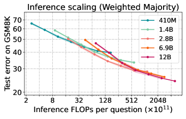
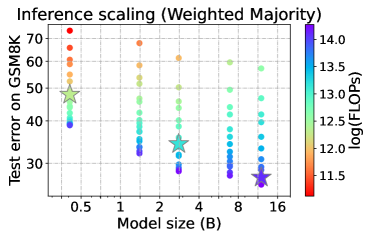
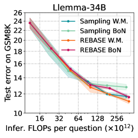
Our results on Pythia (Fig. 1) illustrate the scaling effect of inference compute budget across various model sizes. Typically, increasing computation leads to higher accuracy until the accuracy reaches saturation. As the computation budget increases, the smaller model initially performs better than the larger ones. Once the accuracy of the smaller models saturates, the larger models begin to show their capability. The right panel of Figure 1 demonstrates that the optimal model size for inference varies with different levels of computation. However, in real-world deployment, the available computation is typically much lower than the point where the accuracy of relatively small models saturates and larger models begin to show their advantage (as shown in Figure 4, where the 7B model outperforms the 34B model until 128 Llemma 7B solutions are sampled). This indicates that relatively smaller models could be more compute-optimal for inference.

We have also found that the commonly-used MCTS method does not perform well with weighted voting, as it often yields many unfinished solutions, hence having less effective votes. To address this issue, we propose a novel tree search algorithm, REward BAlanced SEarch (REBASE), which pairs well with weighted voting and improves the Pareto-optimal trade-off between accuracy and inference compute. The key idea of REBASE is to use a node-quality based reward to control the exploitation and pruning properties of tree search, while ensuring enough candidate solutions for voting or selection.

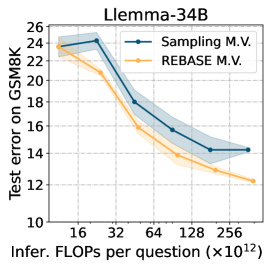
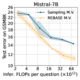
In our experiments, REBASE consistently outperforms sampling and MCTS methods across all settings, models, and tasks. Importantly, we find that REBASE with a smaller language model typically achieves a Pareto-optimal trade-off. For instance, we show that the Llemma-7B model can achieve competitive accuracy to a Llemma-34B model while using $2\times$ less FLOPs when evaluating on MATH500 (Fig. 4) or GSM8K (Fig. 5). These findings underscore the advantages of using smaller models with advanced inference-time algorithms on end-devices to improve problem-solving.

2 Related Works

Mathematical Reasoning with LLMs.

Large language models have made significant progress in recent years, and have exhibited strong reasoning abilities (Brown et al., 2020; Hoffmann et al., 2022; Chowdhery et al., 2022; Lewkowycz et al., 2022). Mathematical problem solving is a key task for measuring LLM reasoning abilities (Cobbe et al., 2021a; Hendrycks et al., 2021b). (Ling et al., 2017) first developed the method of producing step by step solutions that lead to the final answer. Later, (Cobbe et al., 2021b) extended the work by finetuning the pre-trained language model on a large dataset to solve math word problems, a verifier is trained for evaluating solutions and ranking solutions. Nye et al. (2021) train models to use a scratchpad and improve their performance on algorithmic tasks. Wei et al. (2022) demonstrate that the reasoning ability of a language model can be elicited through the prompting. Subsequent research (Kojima et al., 2022; Lewkowycz et al., 2022; Zhou et al., 2022) in reasoning tasks has also highlighted the efficacy of rationale augmentation. We choose problem solving in mathematics as the task to study the compute-optimal strategy since it allows us to accurately evaluate the problem solving ability of LLMs.

Inference Strategies of LLM Problem Solving.

A variety of inference (also called decoding) strategies have been developed to generate sequences with a trained model. Deterministic methods such as greedy decoding and beam search (Teller, 2000; Graves, 2012) find highly probable sequences, often yielding high quality results but without diversity. Sampling algorithms (e.g., temperature sampling (Ackley et al., 1985)) can produce a diverse set of results which are then aggregated to achieve higher accuracy (e.g., via Majority Voting (Wang et al., 2022a)). Recent methods combine search algorithms with modern LLMs, including breadth-first or depth-first search (Yao et al., 2023), Monte-Carlo Tree Search (MCTS) (Zhang et al., 2023; Zhou et al., 2023; Liu et al., 2024; Choi et al., 2023), and Self-evaluation Guided Beam Search (Xie et al., 2023). All of these methods show that using search at inference time can lead to performance gains in various tasks.. However, the trade-off for the improved performance is the use of compute to perform the search. Analyzing the trade-off between compute budget and LLM inference performance remains understudied. In this paper, we systematically analyze the trade-off between compute budget and problem-solving performance, and propose a tree search method that is empirically Pareto-optimal. .

Process Reward Models.

Process reward models (PRMs) have emerged as a technique to improve the reasoning and problem-solving capabilities of LLMs. These models assign rewards to the intermediate steps of the LLM generated sequences. PRMs have been shown effective in selecting reasoning traces with a low error rate, and for providing rewards in reinforcement learning-style algorithms (Uesato et al., 2022; Polu and Sutskever, 2020; Gudibande et al., 2023). Ma et al. (2023) applies the PRM to give rewards on the intermediate steps and guide the multi-step reasoning process. The PRM can be either trained on human labeled data (Lightman et al., 2023a) or model-labeled synthetic data (Wang et al., 2023). In our work, we use the PRM as the reward model for selecting generated solutions, and for selecting which partial solutions to explore in tree search.

Figure 2: Illustration of compute-optimal scaling laws in training and inference. The Chinchilla scaling law (Hoffmann et al., 2022) shows how to choose a model size and number of training tokens under a training-compute budget, while our work shows how to choose a model size and an inference strategy under a inference-compute budget.

3 Compute-Optimal Inference for Problem-Solving

3.1 Problem Formulation

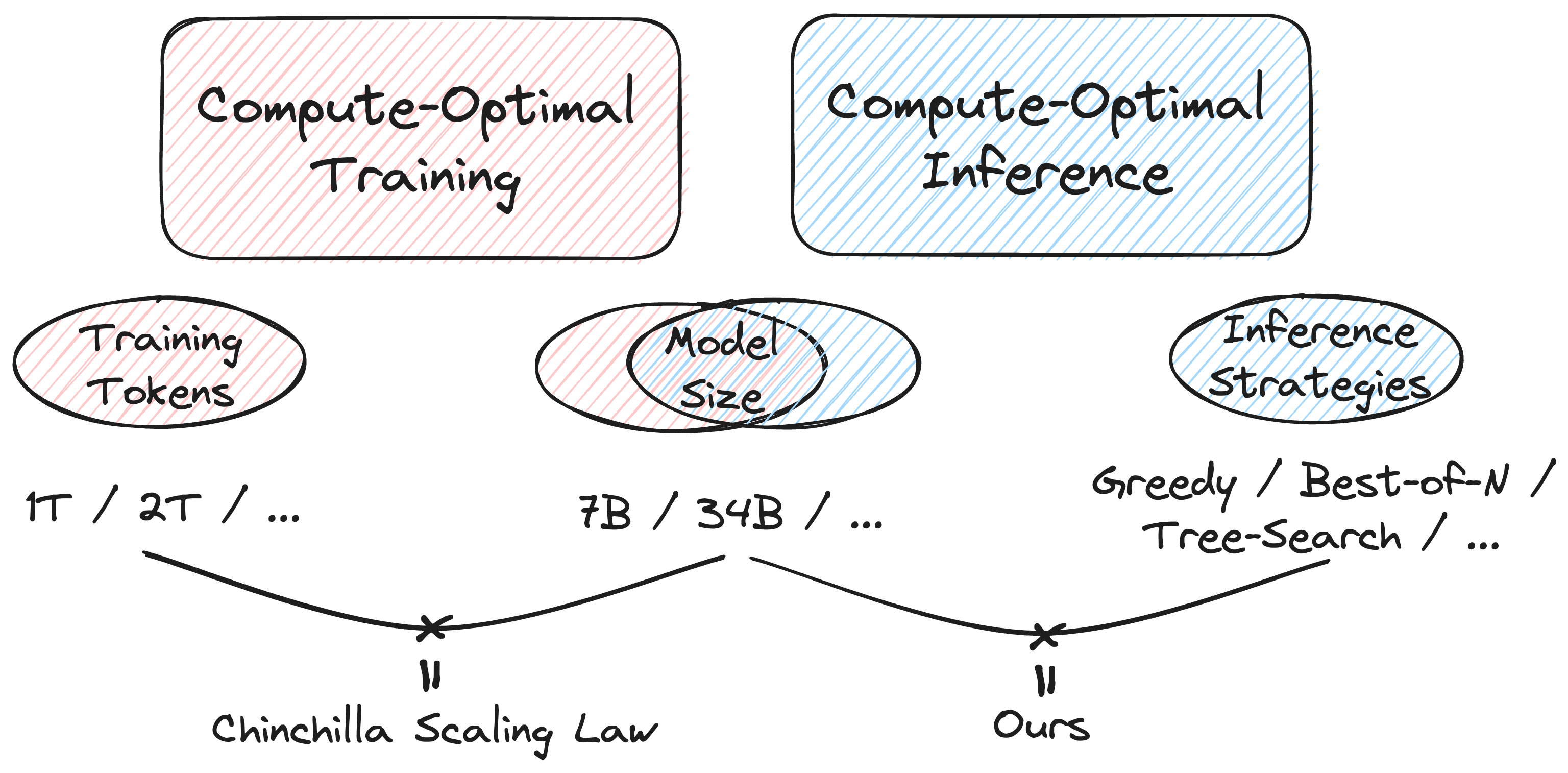
We explore the following question: Given a fixed FLOPs budget, how should one select an optimal model size for the policy model, and an effective inference strategy to maximize performance (i.e., accuracy)? We are the first to formulate this problem and study the inference time scaling law, setting our work apart from previous scaling law studies (Fig. 2).

To address this, we represent the problem-solving error rate $E(N,T;{\mathcal{S}})$ as a function of the number of model parameters $N$, the number of generated tokens $T$ and the inference strategy ${\mathcal{S}}$. The computational budget $C$ is a deterministic function $\text{FLOPs}(N,T;{\mathcal{S}})$, based on $N$ and $T$. Our goal is to minimize $E$ under the test-time compute constraint $\text{FLOPs}(N,T,{\mathcal{S}})=C$:

$$(N_{\mathrm{opt}}(C),T_{\mathrm{opt}}(C);{\mathcal{S}})=\operatorname*{arg\,min}_{(N,T,{\mathcal{S}})\ \text{s.t.}\ \text{FLOPs}(N,T,{\mathcal{S}})=C}E(N,T;{\mathcal{S}})$$

where $N_{\mathrm{opt}}(C)$ and $T_{\mathrm{opt}}(C)$ denote the optimal allocation of a computational budget $C$.

Here, the inference computation (FLOPs) for a fixed model can be modulated by generating more tokens with the policy model, e.g., by sampling additional candidate solutions and subsequently ranking them using a reward model. We primarily consider sampling and tree-search approaches with reranking or Majority Voting as the means to consume more tokens, including Greedy Search, Majority Voting, Best-of-N, Weighted Voting, and their variants on tree search methods.

3.2 Inference Strategies

3.2.1 Sampling-based Methods

We consider the following sampling-based inference strategies which are popularly used in practice:

• Greedy Search. This strategy generates tokens one at a time by selecting the highest probability token at each step, without considering future steps. It is computationally efficient but often suboptimal in terms of diversity.

• Best-of-N. This strategy, also known as rejection sampling, samples multiple solutions and chooses the one with the highest score given by the reward model.

• Majority Voting. In this strategy, multiple model outputs are generated, and the final answer to the problem is determined by the most frequently occurring answer in all the outputs.

• Weighted Majority Voting. This strategy is a variant of Majority Voting in which the votes are weighted based on the scores given by the reward model.

Theoretical Analysis.

Before diving into more sophisticated inference algorithms (e.g., tree search), we present theoretical results on the asymptotic behavior of voting-based strategies given infinite compute in Theorems 1 & 2. Informally, we show that the accuracy of standard/Weighted Majority Voting converges with infinite samples, and the limit only depends on the distribution modeled by the language model (and the reward model). This theoretical finding is also aligned with our empirical findings shown in Sec. 4.2. The proofs are presented in Appendix A.

Notations and assumptions.

Let ${\mathcal{V}}$ be a finite vocabulary and ${\mathcal{V}}^{*}$ its Kleene closure, i.e., the set of all strings. Given a problem $x$, we say a language model answers $y$ to this problem if the model outputs $r\mathrm{e}y$ where $r\in{\mathcal{V}}^{*}$ can be any “reasoning path” and $\mathrm{e}\in{\mathcal{V}}$ denotes a special token that marks the end of reasoning. We further assume that the answer string is always shorter than $L$ tokens, i.e., $|y|\leq L$ for some fixed $L\in{\mathbb{N}}^{*}$ where $|y|$ denotes the length of $y$. For a language model $\pi$, denote by $\pi(v|w)$ the probability of generating $v$ given input (prompt) $w$. For a reward model $\rho$, denote by $\rho(v)$ the score it assigns to the string $v$. We use ${\mathbb{I}}$ to denote the indicator function.

Theorem 1.

Consider a dataset ${\mathcal{D}}=\{(x_{i},y_{i})\}_{i=1}^{m}$ where $x_{i}$ and $y_{i}$ denotes input and true answer, respectively. For a language model $\pi$, denote by $\mathrm{acc}_{n}^{\mathrm{MV}}({\mathcal{D}};\pi)$ the accuracy on ${\mathcal{D}}$ using Majority Voting with $n$ samples. Following the notations and assumptions defined above, we have:

$$\lim_{n\to+\infty}\mathrm{acc}_{n}^{\mathrm{MV}}({\mathcal{D}};\pi) =\frac{1}{m}\sum_{i=1}^{m}{\mathbb{I}}\left[y_{i}=\operatorname*{arg\,max}_{|y|\leq L}\sum_{r\in{\mathcal{V}}^{*}}\pi(r\mathrm{e}y|x_{i})\right]\text{(almost surely);}$$

$$\text{and}\quad\mathbb{E}\left[\mathrm{acc}_{n}^{\mathrm{MV}}({\mathcal{D}};\pi)\right] =\frac{1}{m}\sum_{i=1}^{m}{\mathbb{I}}\left[y_{i}=\operatorname*{arg\,max}_{|y|\leq L}\sum_{r\in{\mathcal{V}}^{*}}\pi(r\mathrm{e}y|x_{i})\right]-\mathcal{O}(c^{-n})$$

for some constant $c>1$.

Theorem 2.

Consider a dataset ${\mathcal{D}}=\{(x_{i},y_{i})\}_{i=1}^{m}$. For a language model $\pi$ and a reward model $\rho$, denote by $\mathrm{acc}_{n}^{\mathrm{WV}}({\mathcal{D}};\pi,\rho)$ the accuracy on ${\mathcal{D}}$ using Weighted Majority Voting with $n$ samples. Following the notations and assumptions defined above, we have:

$$\lim_{n\to+\infty}\mathrm{acc}_{n}^{\mathrm{WV}}({\mathcal{D}};\pi,\rho) =\frac{1}{m}\sum_{i=1}^{m}{\mathbb{I}}\left[y_{i}=\operatorname*{arg\,max}_{|y|\leq L}\sum_{r\in{\mathcal{V}}^{*}}\pi(r\mathrm{e}y|x_{i})\rho(x_{i}r\mathrm{e}y)\right]\text{(almost surely);}$$

$$\text{and}\quad\mathbb{E}\left[\mathrm{acc}_{n}^{\mathrm{WV}}({\mathcal{D}};\pi,\rho)\right] =\frac{1}{m}\sum_{i=1}^{m}{\mathbb{I}}\left[y_{i}=\operatorname*{arg\,max}_{|y|\leq L}\sum_{r\in{\mathcal{V}}^{*}}\pi(r\mathrm{e}y|x_{i})\rho(x_{i}r\mathrm{e}y)\right]-\mathcal{O}(c^{-n})$$

for some constant $c>1$.

Remarks.

Theorems 1 & 2 state the convergence of the accuracy with increasing number of samples, indicating that the performance gains of using more samples will saturate for any fixed models. The limit is determined by the likelihood of generating the correct answers through all possible reasoning paths (and the likelihood should be viewed as a weighted sum for Weighted Majority Voting). This motivates us to consider inference algorithms that search for “good” reasoning paths, such as the tree-search-based variants detailed in Sec. 3.2.2 & 3.2.3.

Theorem 1 & 2 also present insights to compare standard Majority Voting with Weighted Majority Voting. Informally, as long as the reward model is “better than random”, i.e., assigning higher rewards to correct solutions on average, the accuracy limit of Weighted Majority Voting is higher than that of Majority Voting. In our experiments, we consistently find that Weighted Majority Voting dominates Majority Voting. Thus, we focus on Best-of-N and Weighted Majority Voting in the main paper and defer Majority Voting results to Appendix D.

3.2.2 Monte Carlo Tree Search (MCTS)

Monte Carlo Tree Search (MCTS) has proven effective in domains such as board games where strategic decision-making is required (Silver et al., 2016, 2017; Jones, 2021). Recent work has shown that adapting MCTS to the context of LLMs can enhance the text generation process (Zhang et al., 2023; Zhou et al., 2023; Liu et al., 2024; Choi et al., 2023; Chen et al., 2024a; Tian et al., 2024; Chen et al., 2024a). In this context, MCTS is often paired with a value model to score and guide the exploration steps. For additional background, we provide a review of MCTS in Appendix B.

Recent work in MCTS or its variants (e.g., Tree of Thoughts (Yao et al., 2023)) mainly focus on improving the performance (e.g., accuracy) on the studied tasks. However, generic comparisons of MCTS with conventional methods like Best-of-N and Majority Voting in terms of computational budget, measured in generated tokens or processing time, are either scarce or indicating inference-time issues. For example, MCTS consumes substantially more resources, often requiring dozens of times more generated tokens than simpler methods. Specifically, a significant portion of the paths in the search tree are used to estimate and select nodes, and these paths do not necessarily become a part of the final candidate solution, although MCTS ensures that the sampled solutions comprise high-quality intermediate steps. In contrast, sampling methods generate multiple solutions in parallel and independently, and all the generated sequences are included in the candidate solutions. However, the intermediate steps in these sequences are not guaranteed to be of high quality, as there is no mechanism for pruning poor steps or exploiting promising ones.

This highlights the need for developing a new tree search method that can achieve a comparable (or better) performance as MCTS, and that is computationally less costly, just like Weighted Majority Voting and best-of-N. This need motivates the development of our new method named Reward Balanced SEarch (REBASE), as is introduced next.

3.2.3 Reward Balanced Search (REBASE)

Figure 3: Illustration of one iteration of REward BAlanced SEarch (REBASE).

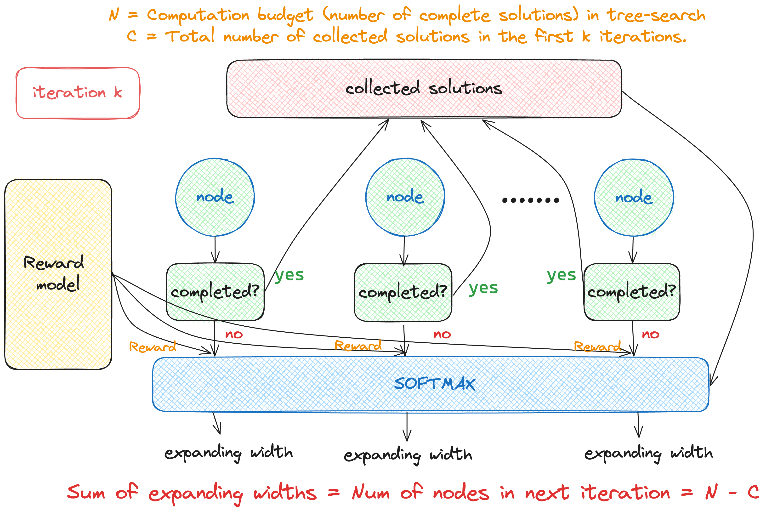
The REBASE tree search method, illustrated in Fig. 3, inherits the exploitation and pruning properties of tree search, while using the reward model alone to estimate the nodes’ qualities without additional computation for estimating values by sampling children. The efficiency is achieved by constraining the total expansion width of the tree at a certain depth. REBASE balances the expansion width among the nodes at the same depth based on the rewards given by the Process Reward Model (PRM). The details are provided below:

Notations. We view the fine-tuned LLM as a policy $\pi_{\theta}$ which generates the solution step by step. Given a question $x$ and the first $k$ steps of a solution $r_{1}\cdots r_{k}$, the $(k+1)$-th step is sampled from $\pi_{\theta}(\cdot|xr_{1}\cdots r_{k})$. REBASE effectively generates a solution tree during inference, in which the root node the question $x$ and other nodes corresponds to solution steps. When generating solution trees, we generate children of $r_{k}$ by sampling from $\pi_{\theta}(\cdot|xr_{1}\cdots r_{k})$. Here we slightly abuse notations and use the corresponding question/solution step to denote a node. The reward of a node $r_{k}$ is generated by the PRM: $R(r_{k}):=R(qr_{1}\cdots r_{k})$.

Initialization. Given the question $x$, balance temperature $T_{b}>0$, and sampling number of solutions $N$, we sample $N$ instances of the first step for the question, yielding all the nodes of depth 1 in the search tree. We let the sampling budget of depth 0, $B_{0}$, to $N$ at initialization.

Reward modeling and update. In the $i$-th iteration, the PRM assigns the rewards to all the nodes at depth $i$. After that, the algorithm examines whether the solutions up to depth $i$ are complete. Supposing there are $C_{i}$ completed solutions, we update the sampling budget using $B_{i}\leftarrow B_{i-1}-C_{i}$. If $B_{i}=0$, the process ends, and we obtain $N$ solutions.

Exploration balancing and expansion. For all of the nodes $n_{j}$ with reward $R(n_{j})$ in the depth $i$ of the tree, we calculate the expansion width of the $n_{j}$ as:

$$W_{j}=\text{Round}\left(B_{i}\frac{\exp\left({R(n_{j})/T_{b}}\right)}{\sum_{k}\exp{\left(R(n_{k})/T_{b}\right)}}\right).$$

Then we sample $W_{j}$ children for $n_{j}$ for all the nodes in depth $i$, and start the next iteration.

4 Experiments

Figure 4: The inference computation scaling comparisons across model sizes. The left/right panel shows the problem-solving error rate on MATH based on Weighted Mjority/Best-of-N.

Figure 5: The inference computation scaling comparisons across model sizes. The left/right panel shows the problem-solving error rate on GSM8K based on Weighted Mjority/Best-of-N. MCTS is not included in the comparison because of its poor compute-accuracy trade-off.

4.1 Setup

Datasets.

We conduct experiments on two mathematical problem-solving datasets to investigate the scaling effects of computation and our REBASE method for both challenging and simpler problems. Specifically, MATH (Hendrycks et al., 2021a) and GSM8K (Cobbe et al., 2021b) are datasets containing high school mathematics competition-level problems and grade-school level mathematical reasoning problems, respectively. Following (Lightman et al., 2023b; Wang et al., 2024; Sun et al., 2024), we use the MATH500 subset as our test set.

Policy model (generators).

To study the inference compute scaling effect, we choose Pythia (Biderman et al., 2023) as our base models since various model sizes are available in the Pythia family. For tree search, we use math-specialized Llemma models (Azerbayev et al., 2024). We further finetune these models on the MeatMath dataset (Yu et al., 2024) using full parameter supervised fine-tuning (Full-SFT), The detailed finetuning configuration is given in the Appendix. Additionally, we test the Mistral-7B (Jiang et al., 2023) to expand our findings across different models and architectures.

Reward Model.

All of the experiments use the same Llemma-34B reward model, which we finetuned on the synthetic process reward modeling dataset, Math-Shepherd (Wang et al., 2024). We added a reward head to the model, enabling it to output a scalar reward at the end of each step.

Inference Configuration.

We use sampling and tree search methods to generate multiple samples and select the answer through Best-of-N, Majority Voting, or Weighted Voting. Each configuration has been run multiple times to calculate the mean and variance, thereby mitigating the randomness and ensuring the reliability of our conclusions.

4.2 Main Results of Compute-Optimal Inference

In order to compare the compute budgets of different models, we plot the figures with the number of FLOPs used per question during inference. We compute the inference FLOPs based on the standard formula from (Kaplan et al., 2020).

Scaling law of compute-optimal inference.

The scaling effect of inference computation budget across different model sizes is shown in Fig. 1. We note that the error rate first decreases steadily and then starts to saturate. Where smaller model first takes advantage since it can generate more samples given limited budget, larger models are preferable with more FLOPs due to the saturation of small model performances. As highlighted in the right panel of Fig. 1, the optimal model size can be different under various computation budgets. We performed a regression analysis on inference FLOPs $C$ and corresponding model sizes $N$ to establish a relationship between a given computational budget and its optimal model size. The resulting regression equation, $\log_{10}\left(C\right)=1.19\log_{10}\left(N\right)+2.03$, enables us to estimate the optimal inference model size for a specified computational constraint.

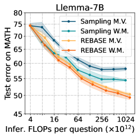
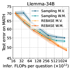
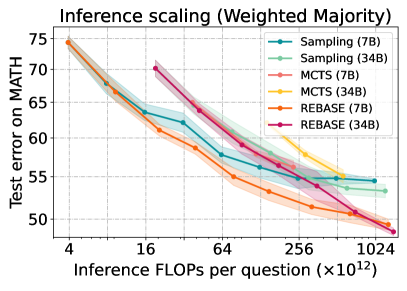
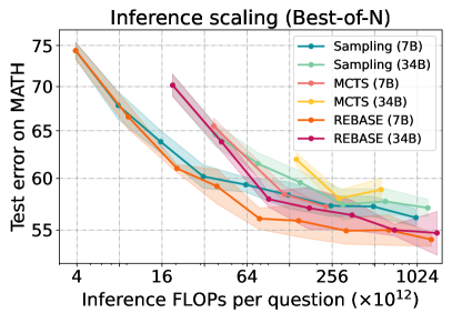
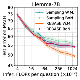
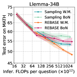
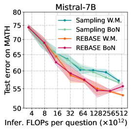
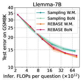
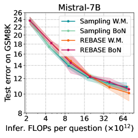
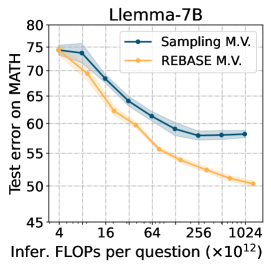
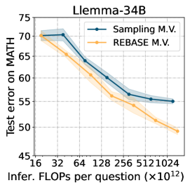
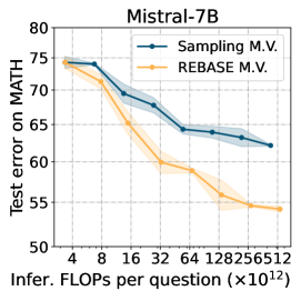
Llemma-7B model achieves competitive accuracy to Llemma-34B model with lower compute budget.

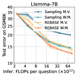
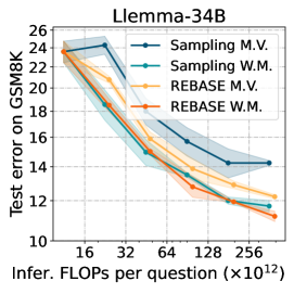
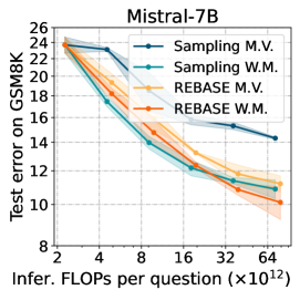
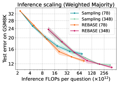
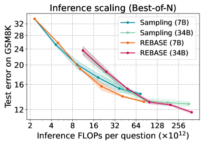
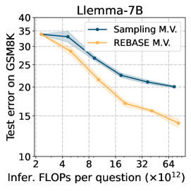
Fig. 4 & 5 show the curves of error rates versus total number of inference FLOPs per question. Inference methods with different model sizes are plotted in the same diagram. We found that Llemma-7B costs approximately $2\times$ less total FLOPs than Llemma-34B under the same method (Sampling, MCTS, REBASE) and task (MATH, GSM8K) while achieving competitive accuracy. This result suggests that, with the same training dataset and model family, training and inference with a smaller model could be more favorable in terms of compute budget if multiple sampling or search methods are employed.

Figure 6: The inference computation scaling laws of different models for the problem-solving error rate on MATH500 test set. The tested models are Llemma-7B (left), Llemma-34B (middle), & Mistral-7B (right). In the legend, W.M. and BoN refer to Weighted Majority and Best-of-N, respectively.

Figure 7: The inference computation scaling laws of different models for the problem-solving error rate on GSM8K test set. The tested models are Llemma-7B (left), Llemma-34B (middle), & Mistral-7B (right). In the legend, W.M. and BoN refer to Weighted Majority and Best-of-N, respectively.

Table 1: REBASE with lower compute budget has competitive accuracy against Sampling with higher compute budget. We use weighted voting to aggreagte the candidate solutions in both Sampling and REBASE.

	# Samples	FLOPs	MATH500
Mistral-7B
Sampling	256	$8.70\times 10^{14}$	42.8
REBASE	32	$\mathbf{1.36\times 10^{14}}$	45.0
Llemma-7B
Sampling	256	$10.0\times 10^{14}$	45.5
REBASE	32	$\mathbf{1.48\times 10^{14}}$	46.8
Llemma-34B
Sampling	64	$12.1\times 10^{14}$	46.7
REBASE	32	$\mathbf{7.08\times 10^{14}}$	49.2

4.3 Comparing REBASE to Other Baselines

REBASE is Pareto-optimal.

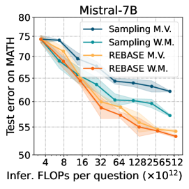
While MCTS undeperforms Sampling (Fig. 4), from Fig. 4, 5, 6, and 7, we found that REBASE consistently outperforms the Sampling method in all settings, when fixing the model and the evaluation task. Table 1 shows that REBASE can achieve competitive accuracy with even a lower compute budget than the sampling method. This finding is novel, and differs from previous tree search works which typically improve the performance at the cost of higher computational expense compared to sampling (Chen et al., 2024a; Xie et al., 2023). Table 2 shows that given the same compute budget (sampling 32 solutions for the 7B model and 8 solutions for 34B model), using REBASE yields higher accuray than sampling.

Table 2: Accuracy of diffrent inference configurations under a specific compute budget. MV, BoN and WV denote Majority Voting, Best-of-N and Weighted Voting, respectively.

	# Samples	MATH FLOPs	GSM8K FLOPs	MATH500	GSM8K
Mistral-7B
Greedy	1	$3.4\times 10^{12}$	$2.3\times 10^{12}$	28.6	77.9
Sampling + MV	32	$109.2\times 10^{12}$	$72.6\times 10^{12}$	36.1	85.7
Sampling + BoN	32	$109.2\times 10^{12}$	$72.6\times 10^{12}$	40.3	89.4
Sampling + WV	32	$109.2\times 10^{12}$	$72.6\times 10^{12}$	39.7	89.1
REBASE + MV	32	$136.2\times 10^{12}$	$78.9\times 10^{12}$	44.1	88.8
REBASE + BoN	32	$136.2\times 10^{12}$	$78.9\times 10^{12}$	45.4	89.4
REBASE + WV	32	$136.2\times 10^{12}$	$78.9\times 10^{12}$	45.0	89.8
Llemma-7B
Greedy	1	$3.92\times 10^{12}$	$2.3\times 10^{12}$	30.0	68.5
Sampling + MV	32	$125.4\times 10^{12}$	$73.9\times 10^{12}$	41.0	80.0
Sampling + BoN	32	$125.4\times 10^{12}$	$73.9\times 10^{12}$	41.7	85.6
Sampling + WV	32	$125.4\times 10^{12}$	$73.9\times 10^{12}$	43.5	85.4
REBASE + MV	32	$148.0\times 10^{12}$	$82.6\times 10^{12}$	46.1	86.1
REBASE + BoN	32	$148.0\times 10^{12}$	$82.6\times 10^{12}$	44.1	86.9
REBASE + WV	32	$148.0\times 10^{12}$	$82.6\times 10^{12}$	46.8	87.3
Llemma-34B
Greedy	1	$19.0\times 10^{12}$	$11.2\times 10^{12}$	33.0	78.4
Sampling + MV	8	$152.3\times 10^{12}$	$89.7\times 10^{12}$	39.9	84.3
Sampling + BoN	8	$152.3\times 10^{12}$	$89.7\times 10^{12}$	40.4	86.7
Sampling + WV	8	$152.3\times 10^{12}$	$89.7\times 10^{12}$	41.0	86.0
REBASE + MV	8	$176.8\times 10^{12}$	$98.7\times 10^{12}$	43.9	86.1
REBASE + BoN	8	$176.8\times 10^{12}$	$98.7\times 10^{12}$	43.6	86.9
REBASE + WV	8	$176.8\times 10^{12}$	$98.7\times 10^{12}$	42.9	86.9

Weaker models gain more from Tree Search.

For example, our proposed REBASE leads to $5.3\%$, $3.3\%$, and $2.6\%$ performance gains on MATH for Mistral-7B, Llemma-7B, Llemma-34B, respectively. The order of accuracy increase is inversely related to the model’s corresponding greedy search on those datasets. This suggests that weaker models, as indicated by their lower greedy search accuracy, benefit more from tree search methods like REBASE.

REBASE saturates later than sampling with higher accuray.

From Fig. 6 and Fig. 7, we observe that both sampling and REBASE saturate early in GSM8K and relatively late in MATH, which we attribute to the difference of the difficulty level. This can be explained through the LLM may assign high probability to the true answer in easy problems than those of harder problems, as suggested by Theorems 1 & 2 with their proofs A. On MATH (Fig. 6), we see that REBASE finally saturates with a higher accuracy than sampling. We hypothesize the reason is that REBASE samples the truth answer with higher probability than sampling. And as demonstrated by Theorems 1 & 2, the upper bound becomes higher.

5 Conclusions & Limitations

Conclusions.

In this work, we conducted a comprehensive empirical analysis of compute-optimal inference for problem-solving with language models. We examined the scaling effect of computation during inference across different model sizes and found that while increased computation generally leads to higher performance, the optimal model size varies with the available compute budget. When the computation budget is limited, smaller models can be preferable. Specifically, a small language model can achieve competitive accuracy to a model four times larger while using approximately half the total FLOPs under the same inference methods (Sampling, MCTS, REBASE) and tasks (MATH, GSM8K). Additionally, we introduce our novel tree search method, REBASE, which is more compute-optimal than both sampling methods and Monte Carlo Tree Search (MCTS). REBASE typically achieves higher accuracy while using several times less computation than sampling methods. Our results underscore the potential of deploying smaller models equipped with sophisticated inference strategies like REBASE to enhance problem-solving accuracy while maintaining computational efficiency.

Limitations.

Our experiments specifically targeted mathematical problem-solving tasks. Additionally, our models were primarily trained using the MetaMath dataset. Investigating the impact of different training datasets on the performance and efficiency of compute-optimal inference strategies for mathematical problem-solving would be a valuable direction for future research.

Acknowledgement.

The computation of the experiments is partially supported by Netmind.

Appendix A Omitted Proofs

A.1 Proof of Theorem 1

Proof.

Recall that we assume the answer must be shorter than $L$ tokens. Let ${\mathcal{A}}=\{v\mid|v|\leq L\}$ be the set of all possible answers. Let $\tilde{\pi}(y\mid x)$ be the probability of the language model $\pi$ outputting the answer $y$ to the question $x$ after marginalizing over the “reasoning paths”, i.e.,

$$\tilde{\pi}(y\mid x)=\sum_{r\in{\mathcal{V}}^{*}}\pi(r\mathrm{e}y|x).$$

Given an input $x$, Assume that $y^{*}=\operatorname*{arg\,max}\limits_{y\in{\mathcal{A}}}\tilde{\pi}(y|x)$, $y^{\prime}=\operatorname*{arg\,max}\limits_{y\in{\mathcal{A}}\backslash\{y^{*}\}}\tilde{\pi}(y|x)$, and denote

$$\delta=\tilde{\pi}(y^{*}|x)-\tilde{\pi}(y^{\prime}|x).$$

For any $y$, denote by $f_{n}(y)$ the number of times that the model answers $y$ in the first $n$ samples. Let $E_{n}$ be the event that Majority Voting with $n$ samples does not output $y^{*}$. We note that $E_{n}$ happens only if there exists $y^{\prime\prime}$ such that $f_{n}(y^{\prime\prime})\geq f_{n}(y^{*})$. Therefore, by union bound,

$${\mathbb{P}}(E_{n})\leq {\mathbb{P}}(\exists\leavevmode\nobreak\ y^{\prime\prime}\in{\mathcal{A}}\backslash\{y^{*}\},f_{n}(y^{\prime\prime})\geq f_{n}(y^{*}))$$

$$\leq \sum_{y^{\prime\prime}\in{\mathcal{A}}\backslash\{y^{*}\}}{\mathbb{P}}(f_{n}(y^{\prime\prime})\geq f_{n}(y^{*}))$$

$$\leq |\mathcal{A}|{\mathbb{P}}(f_{n}(y^{\prime})\geq f_{n}(y^{*}))$$

Note that $f_{n}(y^{*})-f_{n}(y^{\prime})$ can be viewed as a sum of $n$ i.i.d. random variables, which take value $1$ with probability $\tilde{\pi}(y^{*}|x)$, $-1$ with probability $\tilde{\pi}(y^{\prime}|x)$, and $0$ otherwise. Thus, their expectations are all $\delta=\tilde{\pi}(y^{*}|x)-\tilde{\pi}(y^{\prime}|x)$. By Hoeffding’s inequality, we have

$${\mathbb{P}}(f_{n}(y^{\prime})\geq f_{n}(y^{*}))\leq\exp\left(-\frac{n\delta^{2}}{2}\right).$$

Thus,

$${\mathbb{P}}(E_{n})\leq|\mathcal{A}|\exp\left(-\frac{n\delta^{2}}{2}\right)\quad\Rightarrow\quad\sum_{n=1}^{+\infty}{\mathbb{P}}(E_{n})<+\infty.$$

By Borel–Cantelli lemma, we have

$${\mathbb{P}}\left(\limsup_{n\to+\infty}E_{n}\right)=0,$$

which implies the following is true almost surely:

$$\exists\leavevmode\nobreak\ N\in{\mathbb{N}}^{*},\text{ such that for any }n\geq N,\leavevmode\nobreak\ y^{*}=\operatorname*{arg\,max}_{y\in{\mathcal{A}}}f_{n}(y)$$

Hence

$$\lim_{n\to+\infty}\mathrm{acc}_{n}^{\mathrm{MV}}(\{(x,y)\};\pi)={\mathbb{I}}\left[y=y^{*}\right]\qquad(\text{almost surely}).$$

Recall the definition of $y^{*}$, the above shows the theorem is true for a dataset with a single example $\{(x,y)\}$. For general datasets ${\mathcal{D}}$ with $m$ examples, one can apply the above argument to each examples and combine the results to conclude the proof of the almost-sure convergence.

Next, we prove the asymptotic result on $\mathbb{E}\left[\mathrm{acc}_{n}^{\mathrm{MV}}(\{{\mathcal{D}}\};\pi)\right]$. We slightly abuse notation for simplicity as follows: We let $y^{*}(x_{i})=\operatorname*{arg\,max}\limits_{y\in{\mathcal{A}}}\tilde{\pi}(y|x_{i})$, $y^{\prime}=\operatorname*{arg\,max}\limits_{y\in{\mathcal{A}}\backslash\{y^{*}(x_{i})\}}\tilde{\pi}(y|x_{i})$, and let

$$\delta_{\min}=\min_{(x_{i},y_{i})\in{\mathcal{D}}}\tilde{\pi}(y^{*}(x_{i})|x_{i})-\tilde{\pi}(y^{\prime}(x_{i})|x_{i}).$$

We denote by $E_{n}(x_{i})$ the event that Majority Voting with $n$ samples does not output $y^{*}(x_{i})$ given input $x_{i}$. Then it’s easy to see that

$${\mathbb{P}}(E_{n}(x_{i}))\leq|\mathcal{A}|\exp\left(-\frac{n\delta_{\min}^{2}}{2}\right)\quad\Rightarrow\quad{\mathbb{P}}(E_{n}(x_{i}))=\mathcal{O}(c^{-n})$$

where $c>1$ is a constant (which does not depend on $i$).

Note that if $\mathrm{acc}_{n}^{\mathrm{MV}}(\{x_{i},y_{i}\};\pi)=1$, we have $y_{i}=y^{*}(x_{i})$ unless $E_{n}(x_{i})$ happens. In other words,

$$\mathrm{acc}_{n}^{\mathrm{MV}}(\{x_{i},y_{i}\};\pi)\leq{\mathbb{I}}\left[y_{i}=y^{*}(x_{i})\right]+{\mathbb{I}}[E_{n}(x_{i})]$$

$$\Rightarrow\quad \left|\mathbb{E}\left[\mathrm{acc}_{n}^{\mathrm{MV}}(\{x_{i},y_{i}\};\pi)\right]-{\mathbb{I}}\left[y_{i}=y^{*}(x_{i})\right]\right|\leq{\mathbb{P}}(E_{n}(x_{i}))=\mathcal{O}(c^{-n}).$$

Taking a summation over the entire dataset ${\mathcal{D}}$ yields

$$\left|\mathrm{acc}_{n}^{\mathrm{MV}}({\mathcal{D}};\pi)-\frac{1}{m}\sum_{i=1}^{m}{\mathbb{I}}\left[y_{i}=y^{*}(x_{i})\right]\right|\leq\frac{1}{m}\sum_{i=1}^{m}{\mathbb{P}}(E_{n}(x_{i}))=\mathcal{O}(c^{-n}),$$

which concludes the proof. ∎

A.2 Proof of Theorem 2

Proof.

The proof is similar to the proof of Theorem 1. We only need to set

$$\tilde{\pi}(y\mid x)=\sum_{r\in{\mathcal{V}}^{*}}\pi(r\mathrm{e}y|x_{i})\rho(x_{i}r\mathrm{e}y).$$

Then the technique in the proof of Theorem 1 immediately applies. ∎

Appendix B MCTS Details

In this section, we present additional background on the Monte Carlo Tree Search (MCTS) algorithm. The MCTS process can be formulated as the following steps:

Selection.

The process begins at the root node. Here, the algorithm recursively selects the child node that offers the highest Upper Confidence Bound applied to Trees (UCT) value, continuing until a node is reached that has not been expanded. The UCT is calculated using the formula

$$UCT(s)=Q(s)+C\sqrt{\frac{\ln{\left(N(\mathrm{Parent}(s))\right)}}{N(s)}},$$

where $Q(s)$ denotes the quality score of node $s$, $N(s)$ is the number of visits to node $s$, $\mathrm{Parent}(s)$ denotes the parent node of $s$, and $C$ is a constant determining the level of exploration.

Expansion and evaluation.

Upon reaching a non-terminal node $s$, the node is expanded by generating multiple child nodes. Each child node $c$ is then evaluated using a value function $V(c)$, which predicts the potential quality of continuing the sequence from node $c$.

Backpropagation.

After evaluation, the algorithm updates the UCT values and the visit counts for all nodes along the path from the selected node back to the root. For any node $n$ in this path, the updates are made as follows:

$$N(n) \leftarrow N(n)+1,$$

$$Q(n) \leftarrow\frac{\left(N(n)-1\right)Q(n)+V(s)}{N(n)}.$$

Appendix C Hyper-parameters

Table 3: Fine-tuning Hyper-parameters: LR refers to the learning rate, BS refers to the batch size. Pythia, Llemma-7B and LLemma-34B are the generators we use in our experiments, RM is short for Reward Model. We only use problems from GSM8K to train the Pythia models.

Model	# Epoch	Dataset	BS	LR	Max Seq Length	Dtype
Pythia-410M	1	MetaMath (GSM8K)	128	8E-5	768	FP32
Pythia-1.4B	1	MetaMath (GSM8K)	128	4E-5	768	FP32
Pythia-2.8B	1	MetaMath (GSM8K)	128	3E-5	768	FP32
Pythia-6.9B	1	MetaMath (GSM8K)	128	2E-5	768	FP32
Pythia-12B	1	MetaMath (GSM8K)	128	1E-5	768	FP32
Llemma-7B	1	MetaMath	128	8E-6	1024	FP32
Llemma-34B	1	MetaMath	128	8E-6	768	FP32
Llemma-34B RM	2	Math-Shepherd	128	1E-5	768	BF16

Finetuning

All the hyperparameters for model fine-tuning can be found in Table 3. We preprocess the MetaMath Dataset to make the solutions in a stepwise format.

Inference

For all the inference strategies, the temperature of the LLM is set to $1.0$. Max tokens for the output is $1024$ and max tokens for one step is $256$. For REBASE, we chose the balance temperature (the softmax temperature in the REBASE algorithm) as $T_{b}=0.1$. For MCTS, we set $C$ in the UCT value as 1 and we expand $4,8,16$ children for the root, 2 children for other selected nodes with total 32, 64, 128 expansions respectively.

Appendix D Supplementary Figures

Figure 8: The inference computation scaling laws of different models for the problem-solving error rate on MATH test set. The tested models are Llemma-7B (left), Llemma-34B (middle), & Mistral-7B (right). In the legend, M.V. refer to Majority Voting.

Figure 9: The inference computation scaling laws of different models for the problem-solving error rate on GSM8K test set. The tested models are Llemma-7B (left), Llemma-34B (middle), & Mistral-7B (right). In the legend, M.V. refer to Majority Voting.

We append the figures about Majority Voting and Majority Voting v.s. Weighted Majority Voting (Fig. 8, 9 ,10, 11) in this section. The experiments show that although the gap between Majority Voting and Weighted Majority Voting on sampling is huge. This gap becomes much smaller if we apply REBASE. This phenomenon can be caused by the selection ability of tree search like REBASE. Once REBASE already samples solutions with high rewards, conducing Weighted Majority Voting gains less since the sampled solutions may all have relatively high and stable rewards compared with those of sampling.

Figure 10: The inference computation scaling laws of different models for the problem-solving error rate on MATH test set. The tested models are Llemma-7B (left), Llemma-34B (middle), & Mistral-7B (right). In the legend, M.V. and W.M. refer to Majority Voting and Weighted Majority, respectively.

Figure 11: The inference computation scaling laws of different models for the problem-solving error rate on GSM8K test set. The tested models are Llemma-7B (left), Llemma-34B (middle), & Mistral-7B (right). In the legend, M.V. and W.M. refer to Majority Voting and Weighted Majority, respectively.

References

- Ackley et al. [1985] David H Ackley, Geoffrey E Hinton, and Terrence J Sejnowski. A learning algorithm for boltzmann machines. Cognitive science, 9(1):147–169, 1985.
- Azerbayev et al. [2023] Zhangir Azerbayev, Hailey Schoelkopf, Keiran Paster, Marco Dos Santos, Stephen McAleer, Albert Q Jiang, Jia Deng, Stella Biderman, and Sean Welleck. Llemma: An open language model for mathematics. arXiv preprint arXiv:2310.10631, 2023.
- Azerbayev et al. [2024] Zhangir Azerbayev, Hailey Schoelkopf, Keiran Paster, Marco Dos Santos, Stephen McAleer, Albert Q. Jiang, Jia Deng, Stella Biderman, and Sean Welleck. Llemma: An open language model for mathematics, 2024.
- Biderman et al. [2023] Stella Biderman, Hailey Schoelkopf, Quentin Anthony, Herbie Bradley, Kyle O’Brien, Eric Hallahan, Mohammad Aflah Khan, Shivanshu Purohit, USVSN Sai Prashanth, Edward Raff, et al. Pythia: A suite for analyzing large language models across training and scaling. arXiv preprint arXiv:2304.01373, 2023.
- Brooks et al. [2024] Tim Brooks, Bill Peebles, Connor Holmes, Will DePue, Yufei Guo, Li Jing, David Schnurr, Joe Taylor, Troy Luhman, Eric Luhman, Clarence Ng, Ricky Wang, and Aditya Ramesh. Video generation models as world simulators. 2024. URL https://openai.com/research/video-generation-models-as-world-simulators.
- Brown et al. [2020] Tom Brown, Benjamin Mann, Nick Ryder, Melanie Subbiah, Jared D. Kaplan, Prafulla Dhariwal, Arvind Neelakantan, Pranav Shyam, Girish Sastry, Amanda Askell, et al. Language models are few-shot learners. Advances in Neural Information Processing Systems, 33:1877–1901, 2020.
- Chen et al. [2024a] Guoxin Chen, Minpeng Liao, Chengxi Li, and Kai Fan. Alphamath almost zero: process supervision without process, 2024a.
- Chen et al. [2024b] Ziru Chen, Michael White, Raymond Mooney, Ali Payani, Yu Su, and Huan Sun. When is tree search useful for llm planning? it depends on the discriminator. arXiv preprint arXiv:2402.10890, 2024b.
- Choi et al. [2023] Sehyun Choi, Tianqing Fang, Zhaowei Wang, and Yangqiu Song. Kcts: Knowledge-constrained tree search decoding with token-level hallucination detection, 2023.
- Chowdhery et al. [2022] Aakanksha Chowdhery, Sharan Narang, Jacob Devlin, Maarten Bosma, Gaurav Mishra, Adam Roberts, Paul Barham, Hyung Won Chung, Charles Sutton, Sebastian Gehrmann, et al. PaLM: Scaling language modeling with pathways. arXiv preprint arXiv:2204.02311, 2022.
- Cobbe et al. [2021a] Karl Cobbe, Vineet Kosaraju, Mohammad Bavarian, Mark Chen, Heewoo Jun, Lukasz Kaiser, Matthias Plappert, Jerry Tworek, Jacob Hilton, Reiichiro Nakano, Christopher Hesse, and John Schulman. Training verifiers to solve math word problems. arXiv preprint arXiv:2110.14168, 2021a.
- Cobbe et al. [2021b] Karl Cobbe, Vineet Kosaraju, Mohammad Bavarian, Mark Chen, Heewoo Jun, Lukasz Kaiser, Matthias Plappert, Jerry Tworek, Jacob Hilton, Reiichiro Nakano, et al. Training verifiers to solve math word problems. arXiv preprint arXiv:2110.14168, 2021b.
- Gao et al. [2023] Leo Gao, John Schulman, and Jacob Hilton. Scaling laws for reward model overoptimization. In International Conference on Machine Learning, pages 10835–10866. PMLR, 2023.
- Graves [2012] Alex Graves. Sequence transduction with recurrent neural networks, 2012.
- Gudibande et al. [2023] Arnav Gudibande, Eric Wallace, Charlie Snell, Xinyang Geng, Hao Liu, Pieter Abbeel, Sergey Levine, and Dawn Song. The false promise of imitating proprietary llms. arXiv preprint arXiv:2305.15717, 2023.
- Hendrycks et al. [2021a] Dan Hendrycks, Steven Basart, Saurav Kadavath, Mantas Mazeika, Akul Arora, Ethan Guo, Collin Burns, Samir Puranik, Horace He, Dawn Song, et al. Measuring coding challenge competence with apps. arXiv preprint arXiv:2105.09938, 2021a.
- Hendrycks et al. [2021b] Dan Hendrycks, Collin Burns, Saurav Kadavath, Akul Arora, Steven Basart, Eric Tang, Dawn Song, and Jacob Steinhardt. Measuring mathematical problem solving with the math dataset. In Thirty-fifth Conference on Neural Information Processing Systems Datasets and Benchmarks Track (Round 2), 2021b.
- Henighan et al. [2020] Tom Henighan, Jared Kaplan, Mor Katz, Mark Chen, Christopher Hesse, Jacob Jackson, Heewoo Jun, Tom B. Brown, Prafulla Dhariwal, Scott Gray, et al. Scaling laws for autoregressive generative modeling. arXiv preprint arXiv:2010.14701, 2020.
- Hestness et al. [2017] Joel Hestness, Sharan Narang, Newsha Ardalani, Gregory Diamos, Heewoo Jun, Hassan Kianinejad, Md Patwary, Mostofa Ali, Yang Yang, and Yanqi Zhou. Deep learning scaling is predictable, empirically. arXiv preprint arXiv:1712.00409, 2017.
- Hoffmann et al. [2022] Jordan Hoffmann, Sebastian Borgeaud, Arthur Mensch, Elena Buchatskaya, Trevor Cai, Eliza Rutherford, Diego de Las Casas, Lisa Anne Hendricks, Johannes Welbl, Aidan Clark, et al. Training compute-optimal large language models. arXiv preprint arXiv:2203.15556, 2022.
- Jiang et al. [2023] Albert Q Jiang, Alexandre Sablayrolles, Arthur Mensch, Chris Bamford, Devendra Singh Chaplot, Diego de las Casas, Florian Bressand, Gianna Lengyel, Guillaume Lample, Lucile Saulnier, et al. Mistral 7b. arXiv preprint arXiv:2310.06825, 2023.
- Jones [2021] Andy L Jones. Scaling scaling laws with board games. arXiv preprint arXiv:2104.03113, 2021.
- Kaplan et al. [2020] Jared Kaplan, Sam McCandlish, Tom Henighan, Tom B. Brown, Benjamin Chess, Rewon Child, Scott Gray, Alec Radford, Jeffrey Wu, and Dario Amodei. Scaling laws for neural language models. arXiv preprint arXiv:2001.08361, 2020.
- Kojima et al. [2022] Takeshi Kojima, Shixiang Shane Gu, Machel Reid, Yutaka Matsuo, and Yusuke Iwasawa. Large language models are zero-shot reasoners. arXiv preprint arXiv:2205.11916, 2022.
- Lewkowycz et al. [2022] Aitor Lewkowycz, Anders Andreassen, David Dohan, Ethan Dyer, Henryk Michalewski, Vinay Ramasesh, Ambrose Slone, Cem Anil, Imanol Schlag, Theo Gutman-Solo, et al. Solving quantitative reasoning problems with language models. arXiv preprint arXiv:2206.14858, 2022.
- Lightman et al. [2023a] Hunter Lightman, Vineet Kosaraju, Yura Burda, Harri Edwards, Bowen Baker, Teddy Lee, Jan Leike, John Schulman, Ilya Sutskever, and Karl Cobbe. Let’s verify step by step. arXiv preprint arXiv:2305.20050, 2023a.
- Lightman et al. [2023b] Hunter Lightman, Vineet Kosaraju, Yura Burda, Harri Edwards, Bowen Baker, Teddy Lee, Jan Leike, John Schulman, Ilya Sutskever, and Karl Cobbe. Let’s verify step by step, 2023b.
- Ling et al. [2017] Wang Ling, Dani Yogatama, Chris Dyer, and Phil Blunsom. Program induction by rationale generation: Learning to solve and explain algebraic word problems. In Proceedings of the 55th Annual Meeting of the Association for Computational Linguistics (Volume 1: Long Papers), pages 158–167, 2017.
- Liu et al. [2024] Jiacheng Liu, Andrew Cohen, Ramakanth Pasunuru, Yejin Choi, Hannaneh Hajishirzi, and Asli Celikyilmaz. Don’t throw away your value model! generating more preferable text with value-guided monte-carlo tree search decoding, 2024.
- Ma et al. [2023] Qianli Ma, Haotian Zhou, Tingkai Liu, Jianbo Yuan, Pengfei Liu, Yang You, and Hongxia Yang. Let’s reward step by step: Step-level reward model as the navigators for reasoning, 2023.
- Nye et al. [2021] Maxwell Nye, Anders Johan Andreassen, Guy Gur-Ari, Henryk Michalewski, Jacob Austin, David Bieber, David Dohan, Aitor Lewkowycz, Maarten Bosma, David Luan, et al. Show your work: Scratchpads for intermediate computation with language models. arXiv preprint arXiv:2112.00114, 2021.
- OpenAI [2023] OpenAI. Gpt-4 technical report, 2023.
- Peebles and Xie [2023] William Peebles and Saining Xie. Scalable diffusion models with transformers. In Proceedings of the IEEE/CVF International Conference on Computer Vision, pages 4195–4205, 2023.
- Polu and Sutskever [2020] Stanislas Polu and Ilya Sutskever. Generative language modeling for automated theorem proving. arXiv preprint arXiv:2009.03393, 2020.
- Rosenfeld et al. [2019] Jonathan S Rosenfeld, Amir Rosenfeld, Yonatan Belinkov, and Nir Shavit. A constructive prediction of the generalization error across scales. arXiv preprint arXiv:1909.12673, 2019.
- Silver et al. [2016] David Silver, Aja Huang, Chris J Maddison, Arthur Guez, Laurent Sifre, George Van Den Driessche, Julian Schrittwieser, Ioannis Antonoglou, Veda Panneershelvam, Marc Lanctot, et al. Mastering the game of Go with deep neural networks and tree search. Nature, 529(7587):484–489, 2016.
- Silver et al. [2017] David Silver, Julian Schrittwieser, Karen Simonyan, Ioannis Antonoglou, Aja Huang, Arthur Guez, Thomas Hubert, Lucas Baker, Matthew Lai, Adrian Bolton, et al. Mastering the game of go without human knowledge. nature, 550(7676):354–359, 2017.
- Sun et al. [2024] Zhiqing Sun, Longhui Yu, Yikang Shen, Weiyang Liu, Yiming Yang, Sean Welleck, and Chuang Gan. Easy-to-hard generalization: Scalable alignment beyond human supervision. arXiv preprint arXiv:2403.09472, 2024.
- Teller [2000] Virginia Teller. Speech and language processing: an introduction to natural language processing, computational linguistics, and speech recognition, 2000.
- Tian et al. [2024] Ye Tian, Baolin Peng, Linfeng Song, Lifeng Jin, Dian Yu, Haitao Mi, and Dong Yu. Toward self-improvement of llms via imagination, searching, and criticizing. arXiv preprint arXiv:2404.12253, 2024.
- Uesato et al. [2022] Jonathan Uesato, Nate Kushman, Ramana Kumar, Francis Song, Noah Siegel, Lisa Wang, Antonia Creswell, Geoffrey Irving, and Irina Higgins. Solving math word problems with process- and outcome-based feedback. arXiv preprint arXiv:2211.14275, 2022.
- Wang et al. [2023] Peiyi Wang, Lei Li, Zhihong Shao, RX Xu, Damai Dai, Yifei Li, Deli Chen, Y Wu, and Zhifang Sui. Math-shepherd: Verify and reinforce llms step-by-step without human annotations. CoRR, abs/2312.08935, 2023.
- Wang et al. [2024] Peiyi Wang, Lei Li, Zhihong Shao, R. X. Xu, Damai Dai, Yifei Li, Deli Chen, Y. Wu, and Zhifang Sui. Math-shepherd: Verify and reinforce llms step-by-step without human annotations, 2024.
- Wang et al. [2022a] Xuezhi Wang, Jason Wei, Dale Schuurmans, Quoc Le, Ed Chi, Sharan Narang, Aakanksha Chowdhery, and Denny Zhou. Self-consistency improves chain of thought reasoning in language models. International Conference on Learning Representations (ICLR 2023), 2022a.
- Wang et al. [2022b] Yizhong Wang, Yeganeh Kordi, Swaroop Mishra, Alisa Liu, Noah A Smith, Daniel Khashabi, and Hannaneh Hajishirzi. Self-instruct: Aligning language model with self generated instructions. arXiv preprint arXiv:2212.10560, 2022b.
- Wei et al. [2022] Jason Wei, Xuezhi Wang, Dale Schuurmans, Maarten Bosma, Ed Chi, Quoc Le, and Denny Zhou. Chain-of-thought prompting elicits reasoning in large language models. NeurIPS, 2022.
- Xie et al. [2023] Yuxi Xie, Kenji Kawaguchi, Yiran Zhao, Xu Zhao, Min-Yen Kan, Junxian He, and Qizhe Xie. Self-evaluation guided beam search for reasoning, 2023.
- Yao et al. [2023] Shunyu Yao, Dian Yu, Jeffrey Zhao, Izhak Shafran, Thomas L Griffiths, Yuan Cao, and Karthik Narasimhan. Tree of thoughts: Deliberate problem solving with large language models. arXiv preprint arXiv:2305.10601, 2023.
- Yu et al. [2022] Jiahui Yu, Yuanzhong Xu, Jing Yu Koh, Thang Luong, Gunjan Baid, Zirui Wang, Vijay Vasudevan, Alexander Ku, Yinfei Yang, Burcu Karagol Ayan, et al. Scaling autoregressive models for content-rich text-to-image generation. arXiv preprint arXiv:2206.10789, 2(3):5, 2022.
- Yu et al. [2024] Longhui Yu, Weisen Jiang, Han Shi, Jincheng Yu, Zhengying Liu, Yu Zhang, James T. Kwok, Zhenguo Li, Adrian Weller, and Weiyang Liu. Metamath: Bootstrap your own mathematical questions for large language models, 2024.
- Zhang et al. [2023] Shun Zhang, Zhenfang Chen, Yikang Shen, Mingyu Ding, Joshua B. Tenenbaum, and Chuang Gan. Planning with large language models for code generation, 2023.
- Zhou et al. [2023] Andy Zhou, Kai Yan, Michal Shlapentokh-Rothman, Haohan Wang, and Yu-Xiong Wang. Language agent tree search unifies reasoning acting and planning in language models, 2023.
- Zhou et al. [2022] Yongchao Zhou, Andrei Ioan Muresanu, Ziwen Han, Keiran Paster, Silviu Pitis, Harris Chan, and Jimmy Ba. Large language models are human-level prompt engineers. arXiv preprint arXiv:2211.01910, 2022.