Advancing Medical Image Segmentation:
Morphology-Driven Learning with Diffusion Transformer

Abstract

Understanding the morphological structure of medical images and precisely segmenting the region of interest or abnormality is an important task that can assist in diagnosis. However, the unique properties of medical imaging make clear segmentation difficult, and the high cost and time-consuming task of labeling leads to a coarse-grained representation of ground truth. Facing with these problems, we propose a novel Diffusion Transformer Segmentation (DTS) model for robust segmentation in the presence of noise. We propose an alternative to the dominant Denoising U-Net encoder through experiments applying a transformer architecture, which captures global dependency through self-attention. Additionally, we propose k-neighbor label smoothing, reverse boundary attention, and self-supervised learning with morphology-driven learning to improve the ability to identify complex structures. Our model, which analyzes the morphological representation of images, shows better results than the previous models in various medical imaging modalities, including CT, MRI, and lesion images. Our code and dataset are publicly available at: https://github.com/ready2drop/DTS

1 Introduction

Medical image segmentation is crucial in improving our understanding of complex anatomy, providing critical insights for accurate medical diagnosis and precise treatment planning. This is especially important in computed tomography(CT) scans, where the intrinsic complexity of medical images presents unique challenges that require sophisticated solutions for organ segmentation. Unlike general images, CT images are quantitative imaging, and pixel intensities are normalized to Hounsfield units (HU) values[Lev and Gonzalez(2002)]. (e.g., air as -1000 HU, bone as +400 to +1000 HU). Therefore, clinicians must understand the quantitative meanings and select the appropriate range to enhance the visual contrast of specific tissues or organs. In particular, research is conducted to find appropriate range values for each tissue or organ in CT scans[Lev and Gonzalez(2002), Raybaud(2020), Adams et al.(2012)Adams, Mughal, Damilakis, and Offiah, Sahi et al.(2014)Sahi, Jackson, Wiebe, Armstrong, Winters, Moore, and Low, Mertens et al.(2023)Mertens, Hecht, Bauknecht, and Vajkoczy] and studies show that segmenting CT images with an inappropriate HU range normalized leads to poor performance[Huo et al.(2019)Huo, Tang, Chen, Gao, Han, Bao, De, Terry, Carr, Abramson, and Landman, Kim and Chun(2020)].

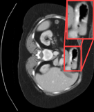
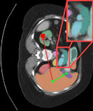
(a)	(b)

Figure 1: Medical imaging drawbacks.

This is because inappropriate normalization can occlude organs, as illustrated in Fig.1 (a). Additionally, clinicians can have different opinions in labeling[Alpert and Hillman(2004), Monteiro et al.(2020)Monteiro, Le Folgoc, Coelho de Castro, Pawlowski, Marques, Kamnitsas, van der Wilk, and Glocker, Becker et al.(2019)Becker, Chaitanya, Schawkat, Muehlematter, Hötker, Konukoglu, and Donati, Joskowicz et al.(2019)Joskowicz, Cohen, Caplan, and Sosna]. Due to this, ground truths are not determinstic, and it may be difficult to obtain detailed representations of organ or lesion labels. Inaccurate manual labeling can further increase the complexity of organ segmentation, as shown in Fig.1 (b). We address intrinsic challenges in medical images with an architecture that combines the advantages of the adaptive and resilient Swin Transformer encoder[Liu et al.(2021)Liu, Lin, Cao, Hu, Wei, Zhang, Lin, and Guo] with the efficient decoder in UNet[Ronneberger et al.(2015)Ronneberger, Fischer, and Brox]. We break away from the conventional Denoising U-Net[Rombach et al.(2022)Rombach, Blattmann, Lorenz, Esser, and Ommer] structure because we need a model that captures a global contextual representation and can handle the various medical imaging data. In addition, we introduce three approaches to improve the segmentation process further. First, distance-aware label smoothing[Yu et al.(2017)Yu, Liu, Gong, Zhang, Batmanghelich, and Tao, Zhang et al.(2023)Zhang, Zheng, Shi, et al., Felfeliyan et al.(2023)Felfeliyan, Hareendranathan, Kuntze, Wichuk, Forkert, Jaremko, and Ronsky] is a guidance mechanism that recognizes anatomical locations in the medical image and smoothes labels by calculating location-based distances. Second, reverse boundary attention captures areas of subtle and ambiguous boundaries. This component contributes to more precise and accurate segmentation by explicitly directing the model attention to edges[Wang et al.(2022)Wang, Chen, Ji, Fan, and Li, Lee et al.(2020)Lee, Kim, Lee, Kim, and Ro], especially in the regions that have not been manually labeled. Third, self-supervised learning[Alzubaidi et al.(2020)Alzubaidi, Fadhel, Al-Shamma, Zhang, Santamaría, Duan, and R. Oleiwi, Ghesu et al.(2022)Ghesu, Georgescu, Mansoor, Yoo, Neumann, Patel, Vishwanath, Balter, Cao, Grbic, and Comaniciu, Shurrab and Duwairi(2022)] allows complex features of organs to capture meaningful representations from input images in a scenario of insufficient data. We reduce reliance on labeled data and improve model adaptability to diverse and complex features of medical images. Our proposed method demonstrates generalizability beyond medical images when we evaluate it with a different domain task that can utilize morphological information. Therefore, our contribution is summarized as follows.

• We presents a new diffusion transformer segmentation(DTS) model which performs better than previous framework(i.e. CNN based Denoising Diffusion Probabilistic Model).

• We introduce a novel approach to address the medical image segmentation by integrating morphology-driven learning into the image processing, such as k-neighbor label smoothing, reverse boundary attention, and self-supervised learning.

• Our model demonstrates the generality in segmentation tasks in medical modalities such as CT, MRI, and lesion images and further suggests that this approach may be adaptable to other domains.

2 Related Work

The diffusion segmentation model which applies the generative diffusion process, allows users to manipulate the ambiguity of each time step through a hierarchical structure, solving the image quality and diversity problems of existing methods, allowing the learning process to proceed stably. There is research that has notable potential applied to medical imaging[Kim et al.(2022)Kim, Oh, and Ye, Guo et al.(2023)Guo, Yang, Ye, Lu, Peng, Huang, Xiang, and Ma, Wolleb et al.(2022)Wolleb, Sandkühler, Bieder, Valmaggia, and Cattin]. SegDiff[Amit et al.(2022)Amit, Shaharbany, Nachmani, and Wolf], which showed consistent performance under various imaging conditions, is the first approach to solving the image segmentation problem by applying diffusion. The feature of this model is a mechanism that integrates the information of the input image and the current estimate of the segmentation map through each encoder and uses the decoder to improve the segmentation map iteratively. MedSegDiff[Wu et al.(2023)Wu, Fu, Fang, Zhang, Yang, Xiong, Liu, and Xu] also applied the diffusion segmentation model to medical image segmentation. The input of the conditional image and noise segmentation map are integrated using a mechanism such as SegDiff, but high-frequency noise is constrained through the Fast Fourier transform module during the connection process. In addition, Diff-UNet[Xing et al.(2023)Xing, Wan, Fu, Yang, and Zhu] implemented the standard U-shaped architecture, which learns from the input volume in medical image segmentation effectively to extract semantic information. Here, we focus on the architecture and compare it with the existing diffusion segmentation model to demonstrate through experiments that the inductive bias, which is a major feature of CNN, can be replaced by ViT in diffusion segmentation.

Label Smoothing for Image Segmentation. Ground truth labeling for image segmentation is a time-consuming and intensive task involving experts. These processes are inherently subjective and susceptible to factors such as image quality, observer diversity, and difficulty depicting specific structures. Moreover, earlier label smoothing methods[Szegedy et al.(2015)Szegedy, Vanhoucke, Ioffe, Shlens, and Wojna, Müller et al.(2020)Müller, Kornblith, and Hinton, Galdran et al.(2020b)Galdran, Chelbi, Kobi, Dolz, Lombaert, ben Ayed, and Chakor, Islam and Glocker(2021), Zhang et al.(2020)Zhang, Jiang, Hou, Wei, Han, Li, and Cheng, Liu et al.(2022)Liu, Ben Ayed, Galdran, and Dolz], the inter-class relationships are usually overlooked since the labels are smoothed into one-hot encoding vectors. To address these challenges, we experimentally highlight the implementation of strategic label smoothing based on the spatial location of organs.

Reverse boundary attention refers to the integration of reverse attention[Huang et al.(2017a)Huang, Xia, Wu, Li, Wang, Song, and Kuo, Lou et al.(2023)Lou, Guan, and Loew], which learns opposite concepts that are not associated with the target class in a way that substitutes existing attention mechanisms for objects, and boundary attention[Ghadimi et al.(2015)Ghadimi, Moghaddam, Grebe, and Wallois, Bai et al.(2016)Bai, Li, and Wang, Shojaii et al.(2005)Shojaii, Alirezaie, and Babyn], which emphasizes pixels or features of parts related to the boundary. This mechanism plays a crucial role in enhancing the performance of object segmentation in medical images. This is particularly important because medical imaging, such as CT and MRI scans, often exhibit ambiguous organ boundaries and significant amounts of noise, posing challenges for accurate segmentation. Therefore, we explore the benefits of combining unique advantages, such as a reverse boundary attention mechanism, into our framework.

3 DTS: Diffusion Transformer Segmentation

The diffusion model is a generative model that consists of two stages: a diffusion process and a denoising process. In the diffusion process, Gaussian noise is added incrementally to the segmentation label $x_{0}$ over a series of steps $t$.

$$p_{\theta}(x_{0:T-1}|x_{T}):=\prod_{t=1}^{T}p_{\theta}(x_{t-1}|x_{t})$$ (1)

$$p_{\theta}(x_{t-1}|x_{t}):=\mathcal{N}(x_{t-1};\mu_{\theta}(x_{t},t),\Sigma_{\theta}(x_{t},t))$$ (2)

The denoising process, parametrized by $\theta$, involves training a neural network to recover the original data from the noise, and the distribution $p_{\theta}(x_{t})$ is defined as $\mathcal{N}(x_{T};0,I_{n\times n})$ where $I$ represents the raw image assumed to be an $n\times n$ matrix. The denoising process then operates to transform the latent variable distribution $p_{\theta}(x_{t})$ (i.e. gaussian noise image) into the data distribution $p_{\theta}(x_{0})$ (i.e. final segmentation map).

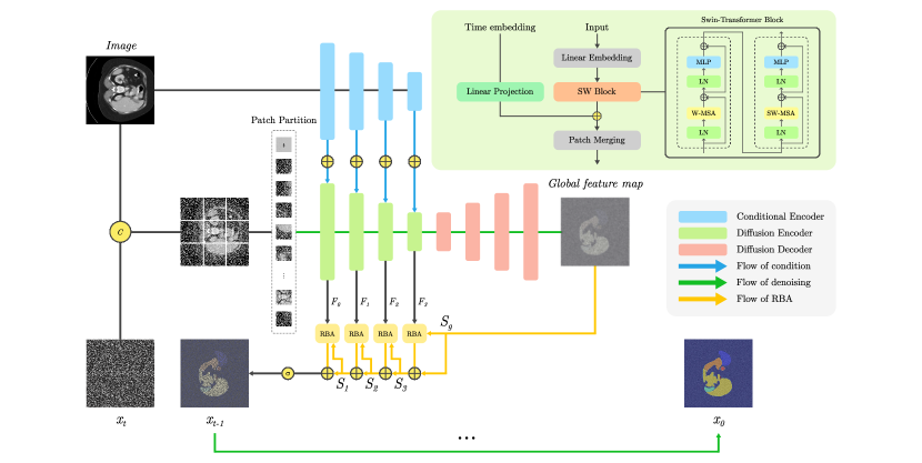
Figure 2: Overview of our proposed diffusion transformer segmentation(DTS) model.

Architecture	Average Accuracy
	Dice $\uparrow$
Denoising U-Net[Rombach et al.(2022)Rombach, Blattmann, Lorenz, Esser, and Ommer]	$79.74\pm 0.30$
Ours(DTS)*	$\textbf{81.12}\pm 0.19$

Table 1: Comparison of an encoder network on the ISIC dataset.

The denoising phase shown in Fig.2 follows the encoder-decoder network structure of standard denoising autoencoder[Rombach et al.(2022)Rombach, Blattmann, Lorenz, Esser, and Ommer]. As shown in Table.1, we empirically suggest the possibility of replacing the latent diffusion encoder with a Swin transformer[Liu et al.(2021)Liu, Lin, Cao, Hu, Wei, Zhang, Lin, and Guo], which has advantages such as scalability and computational efficiency when processing various images due to its hierarchical structure. Also, similar to the conditional mechanism[Mirza and Osindero(2014), Sohn et al.(2015)Sohn, Lee, and Yan, Rombach et al.(2022)Rombach, Blattmann, Lorenz, Esser, and Ommer], our model incorporates another type of conditional encoder, $\tau_{\theta}$ where the original image is used as input. These are demonstrated in the diffusion encoder and conditional encoder in Fig.2. Our method combines information from the current estimate $x_{t}$, the image $I$, and the time step index $t$ to adjust the step estimate function ${\epsilon}_{\theta}$ at the input. It also takes the conditional image $\tau_{\theta}(I)$) and reconstructs it through a UNet decoder to produce the global feature map. Subsequently, the RBA modules facilitate the derivation of the final segmentation map, which exhibits precise edge representation, as detailed in Fig.3. In conclusion, $DTS(\cdot)$ represents our novel diffusion transformer segmentation model, which performs segmentation by integrating the described components.

$${\epsilon}_{\theta}(x_{t},I,t)=DTS((x_{t},I),t,\tau_{\theta}(I))$$ (3)

4 Morphology Driven Learning

$k$-Neighbor Label smoothing by organ distance. We explore medical data from body parts such as the abdomen and brain, which have organs or diseases located structurally within a compact space. As the relative positions of organs do not differ from person to person,

Label smoothing	Average Accuracy
	Dice $\uparrow$	HD $\downarrow$
Scratch	$81.12$	$5.11$
$k$-NLS
$\mathcal{\alpha\text{= 0.1}}$	84.41	4.17
$\mathcal{\alpha\text{= 0.2}}$	$84.35$	$4.20$
$\mathcal{\alpha\text{= 0.3}}$	$83.31$	$4.53$

Table 2: Accuracy changes with different $\alpha$(scale factor) values.

we propose a $k$-neighbor label smoothing method that leverages the relative positions of organs for distance-aware smoothing of the labels of $k$ neighbors for a given class or organ. In a multi-class ($k>2$) situation, such as in this case, there is an advantage if there is a positional relationship between them. The positional relationship refers to the relative positional relationship of organs anatomically. As shown in Fig. 1 (b), the liver($\star$) is close to the gall bladder($\blacktriangle$) but relatively far from the left kidney($\blacksquare$). We provided semantic information to the model based on which body structure would match this prior knowledge. The equation of k-neighbor label smoothing ($k-NLS$) is:

$$d_{t}=\{d_{xyz}\mid x,y,z\in N,x<W,y<H,z<D\}\\$$ (4)

The distance is calculated channel-wise, measuring the distance between a random point and the centroid of $i$th class.

$$y_{t}^{k-NLS}=\left|y_{t}-\frac{\alpha}{d_{t}+\epsilon}\right|\\$$ (5)

where $y_{t}$ is "$1$" for the target class and "$0$" for the rest of all, the label smoothing scale factor $\alpha$ is crucial. Based on previous research[Müller et al.(2020)Müller, Kornblith, and Hinton] and empirical experiments on the BTCV dataset(Table.3), opting for $\alpha$ as 0.1 yields optimal outcomes. $\epsilon$ is constant $1e^{-6}$ to prevent division by zero, and $d_{x,y,z}=\{d_{0},d_{1},...,d_{i}\mid i=k\}$ is a set of centroids and distances between each pixel and class. The pseudo code is expressed as follows:

Algorithm 1 K-Neighbor Label smoothing

Input: label
Parameter: $\epsilon$(constant factor), $\alpha$(scale factor)
Output: smoothed label

1:  Let encoded_label = one_hot_encoding(label)

2:  Let coordinates = meshgrid(W, H, D)

3:  Let centroids = compute_centroids(encoded_label)

4:  Let d = tensor of shape [C, W, H, D]

5:  for each class c in range(C) do

6:     for each (x, y, z) in coordinates do

7:        d[c, x, y, z] = distance((x, y, z), centroids[:, c])

8:     end for

9:  end for

10:  Let smoothed_label = abs(label - $\alpha$ / (d + $\epsilon$))

11:  return  smoothed_label

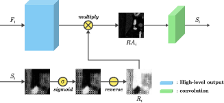
Figure 3: Illustration of the RBA module.

RBA: Reverse-boundary Attention. Complex anatomy and the inherent ambiguity in defining boundaries of adjacent organs are factors that hinder accurate segmentation of organ boundaries in medical images. Considering that these factors are likely to result in false positives or missing details in the initial segmentation, our approach includes selectively dropping or reducing the prediction weights of overlooked regions. The Reverse Boundary Attention method aims to improve the prediction of segmentation models by gradually capturing and specifying areas that may have been initially ambiguous. Thus, our architecture removes previously estimated predictive areas from high-level output features where existing estimates are upsampled in deeper layers, sequentially explores these details, including areas and boundaries, and finally, improves the segmentation model predictions progressively. In the Fig. 2, the global feature map which is the output of the decoder, is resized to match the input size using a convolution layer, and reverse attention[Huang et al.(2017b)Huang, Xia, Wu, Li, Wang, Song, and Kuo] is then performed to obtain the weight $R_{i}$. Multiplying(element-wise $\odot$) this by the high-level output$\{F_{i},i=0,1,2,3\}$ to obtain the output reverse attention $RA_{i}$.

$$R_{i}=\ominus(\sigma(\mathcal{U}(S_{i+1})))$$ (6)

$$RA_{i}=F_{i}\odot R_{i}.$$ (7)

where $\mathcal{U}(\cdot)$, $\sigma(\cdot)$, $\ominus(\cdot)$ is up-sampling, sigmoid, reverse function respectively, The reverse function removes the matrix, which in all the elements is $1$.

As shown below, the reverse attention weight $RA_{i}$ is passed through two convolution layers with normalization and finally the reverse boundary attention $S_{i+1}$ is obtained.

$$S_{i+1}=L_{conv}(RA_{i})$$ (8)

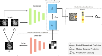
Figure 4: Our proposed SSL framework

Self-supervised learning (SSL) can encode anatomical information of the human body in the image effectively. We propose three proxy tasks for learning comprehensive semantic representations within masked images without using labels. Our framework combines (1) Contrastive learning(e.g. SimCLR[Chen et al.(2020)Chen, Kornblith, Norouzi, and Hinton]), which encodes masked images to improve the ability to distinguish between different samples with hidden feature representations; (2) Masked Location Prediction, which predicts the location of the samples; and (3) Partial Reconstruct Prediction(e.g. SimMIM[Xie et al.(2022)Xie, Zhang, Cao, Lin, Bao, Yao, Dai, and Hu]), which learns the feature representation by reconstructing the masked patch area of each sub-volume. These widely recognized self-supervised learning strategies are both straightforward and effective.

When the input(demonstrated 2D image in Fig.4) is divided into patches and then passed as input to the encoder twice, two sets of latent embeddings are obtained, and a contrastive learning is performed through constrastive loss[van den Oord et al.(2019)van den Oord, Li, and Vinyals] (Eq.9). Then, masked location prediction is conducted to predict the number of randomly masked parts by dividing the $\hat{h_{i}}$ image into patches from 0 to 8 (Eq.10). In addition, Partial Reconstruct Prediction is performed by masking the image of $\hat{h_{j}}$, reconstructing it through a decoder, and learning the difference from the original through $L_{2}$ loss (Eq.11).

$$\mathcal{L}_{\mathrm{CL}}=-\log\frac{\exp\left(\operatorname{sim}\left(x_{i},x_{j}\right)/t\right)}{\sum_{k}^{2N}\mathds{1}_{k\neq i,j}\exp\left(\operatorname{sim}\left(x_{i},x_{k}\right)/t\right)}$$ (9)

$$\mathcal{L}_{\mathrm{Loc}}=-\frac{1}{R}\sum_{n=1}^{R}{v}_{n}log(\hat{v}_{n})$$ (10)

$$\mathcal{L}_{\mathrm{Rec}}=\frac{1}{|\hat{R}|}\sum_{r\in\hat{R}}||y_{r}-\hat{y}_{r}||_{2}$$ (11)

Finally, We minimize total objective loss functions combining partial reconstruction prediction, masked location prediction and contrastive learning losses, as follows:

$$\mathcal{L}_{\mathrm{total}}=\mathcal{L}_{\mathrm{Rec}}+\lambda_{1}\mathcal{L}_{\mathrm{Loc}}+\lambda_{2}\mathcal{L}_{\mathrm{CL}}\vspace{-0.2cm}$$ (12)

where $\lambda_{1},\lambda_{2}$ are set to 0.1 and 0.01 respectively, as a result of empirical experiments.

5 Experiments

Datasets. The pre-training dataset consists of medical images sourced from partial accessible CT, MRI datasets encompassing 3,358, 6,970 subjects respectively. Notably, the pre-training step does not involve the utilization of annotations or labels on this dataset. The primary objective of this pre-training process is to enable the model to learn meaningful representations from the available image data, thus eliminating the need for manual annotation. The BTCV[Landman et al.(2015)Landman, Xu, Igelsias, Styner, Langerak, and Klein] dataset comprises 3D abdominal multi-organ CT images from 30 cases, each associated with a specific form and featuring 13 multi class segmentation objectives. The BraTS2021[Baid et al.(2021)Baid, Ghodasara, Bilello, Mohan, Calabrese, Colak, Farahani, Kalpathy-Cramer, Kitamura, Pati, Prevedello, Rudie, Sako, Shinohara, Bergquist, Chai, Eddy, Elliott, Reade, Schaffter, Yu, Zheng, Annotators, Davatzikos, Mongan, Hess, Cha, Villanueva-Meyer, Freymann, Kirby, Wiestler, Crivellaro, Colen, Kotrotsou, Marcus, Milchenko, Nazeri, Fathallah-Shaykh, Wiest, Jakab, Weber, Mahajan, Menze, Flanders, and Bakas] dataset includes 1,251 subjects of brain MRI images. Each image is annotated with three segmentation targets and encompasses four modalities T1, T1Gd, T2, and T2-FLAIR. The ISIC2018[Cassidy et al.(2022)Cassidy, Kendrick, Brodzicki, Jaworek-Korjakowska, and Yap] dataset contains 2,594 dermoscopic images of skin lesions, each annotated by experts for segmentation purposes. The Cityscapes[Cordts et al.(2016)Cordts, Omran, Ramos, Rehfeld, Enzweiler, Benenson, Franke, Roth, and Schiele] dataset contains several urban street scenes for segmentation purposes and is used to test the generalization performance of our approach. It consists of 3475 semantically annotated train, val sets and 1525 test set. Details about datasets are shown in the appendix.

Implementation Details. Our architecture implemented in PyTorch and MONAI. For pre-training tasks, the reconstruction strategy is applied with a mask ratio of 0.4. Moving on to the fine-tuning phase, the AdamW optimizer[Loshchilov and Hutter(2019)] is used with a weight decay $1e^{-3}$. The warm-up is set to $0.1$ of the total epochs, and the learning rate undergoes linear updates following the Cosine Annealing schedule[Loshchilov and Hutter(2017)]. The loss function incorporates DICE loss[Sudre et al.(2017)Sudre, Li, Vercauteren, Ourselin, and Jorge Cardoso], BCE loss, and MSE loss. Random flips, rotations, intensity scaling, and shifts were applied to augment the data. We set the number of diffusion steps as $1000$, and the sliding window overlap rate is $0.8$ until the final prediction. Preprocessing details for each dataset are provided in the appendix.

Evaluation Metrics are important to quantify the performance of the segmentation model. Two commonly used metrics are the dice similarity coefficient[Zou et al.(2004)Zou, Warfield, Bharatha, Tempany, Kaus, Haker, Wells, Jolesz, and Kikinis](Dice) and the Hausdorff distance[Huttenlocher et al.(1993)Huttenlocher, Klanderman, and Rucklidge](HD). The evaluation metric are as define. $Y$ and $\hat{Y}$ represent the actual and predicted values in input units, and $g^{\prime}$ and $p^{\prime}$ represent the actual and predicted values of points on the surface.

$$\textrm{Dice}=\frac{2\sum_{i=1}^{I}Y_{i}\hat{Y}_{i}}{\sum_{i=1}^{I}Y_{i}+\sum_{i=1}^{I}\hat{Y}_{i}},$$ (13)

$$\textrm{HD}=\max\{{\max_{g^{\prime}\in G}\min_{p^{\prime}\in P}}\|g^{\prime}-p^{\prime}\|,\max_{p^{\prime}\in P}\min_{g^{\prime}\in G}\|p^{\prime}-g^{\prime}\|\}.$$ (14)

Label smoothing	Average Accuracy
	IoU $\uparrow$
LS	$83.72\pm 0.08$
N-ULS [Galdran et al.(2020a)Galdran, Chelbi, Kobi, Dolz, Lombaert, Ben Ayed, and Chakor]	$83.91\pm 0.04$
SVLS[Islam and Glocker(2021)]	$83.79\pm 0.06$
Ours*($k$-NLS)	$\textbf{84.19}\pm 0.04$

Table 3: Comparison with the other LS

Exploring the performance of Label Smoothing We concentrate on the performance of k-neighbor label smoothing and explore its applicability to general datasets with structural properties. We explore its applicability to a cityscapes[Cordts et al.(2016)Cordts, Omran, Ramos, Rehfeld, Enzweiler, Benenson, Franke, Roth, and Schiele] dataset with structural properties by utilizing only our baseline model and label smoothing. Compared with basic label smoothing(uniform), Non-Uniform Label Smoothing(NULS), and especially Spatially Varying Label Smoothing(SVLS), which applies label smoothing to neighboring pixels using weight matrix in the form of Gaussian kernel, we can see that our performance is superior. Previous methods compensate for the label’s uncertainty in image segmentation, but our methods further estimate the positional relationship between classes to improve prediction performance with a label smoothing method, emphasizing that this can be easily applied to other tasks.

Loss Function	Average Accuracy
	Dice $\uparrow$	HD $\downarrow$
Scratch	$81.12$	$5.11$
$\mathcal{L_{\text{CL}}}$	$81.21$	$5.10$
$\mathcal{L_{\text{Loc}}}$	$81.23$	$5.10$
$\mathcal{L_{\text{Rec}}}$	$81.56$	$5.06$
$\mathcal{L_{\text{Rec}}}+\mathcal{L_{\text{CL}}}$	$81.87$	$4.95$
$\mathcal{L_{\text{Rec}}}+\mathcal{L_{\text{Loc}}}$	$81.61$	$4.98$
$\mathcal{L_{\text{Rec}}}+\mathcal{L_{\text{CL}}+}\mathcal{L_{\text{Loc}}}$	$\mathbf{82.19}$	$\mathbf{4.85}$

Table 4: Ablation study of the pre-training objective function

Efficiency of Self Supervised Objectives. We conduct comprehensive ablation experiments on the BTCV dataset to evaluate the efficiency of self-supervised learning. In these experiments, we employed specific settings for calculating the loss, and the obtained results are presented in the Table.4. Notably, the $L_{\text{Rec}}$ is learned based on the pixel representation of input images, $L_{\text{Loc}}$ (Masked Location Prediction) is learned by recognizing the location of the masked region, and $L_{\text{CL}}$ (Contrastive Learning) is focused on contrastive learning at two augmented sample level. The $L_{\text{Rec}}$ lies in its important role in understanding meaningful representation learning from medical images, as shown in experimental results. By employing these three loss functions, our self-supervised learning approach aims to capture intricate details at both pixel and region levels, enhancing the model’s ability to extract meaningful features from the the inputs.

Architecture	Average Accuracy
	Dice $\uparrow$	HD $\downarrow$
Scratch	$81.12$	$5.11$
SSL
Encoder$\mathcal{{}_{\text{Frozen}}}$	$83.17$	$4.55$
Encoder$\mathcal{{}_{\text{Trainable}}}$	$84.67$	$4.11$
RBA	$82.60$	$4.74$
Ours*	86.72	$3.48$

Table 5: Comparing morphology-driven learning strategies

Selecting the optimal architecture Remind the our approaches, in the case of self-supervised learning (SSL), feature representations pre-trained from the three proxy tasks are transferred to the conditional encoder to assist in understanding the original image. We experiment with the effect of freezing or leaving all weights trainable during benchmark fine-tuning. Additionally, our framework explores the ablation study on reverse boundary attention, which is integrated with the general diffusion segmentation process. We comprehensively verify the effectiveness of morphology-driven learning within the architecture to prove its hypothesis. As shown in the Table.5, the single module experiments(presented in the second section) show higher performance than the scratch model, but learning by leaving the conditional encoder trainable shows a large margin in the BTCV dataset. This indicates that feature representation was achieved by aligning the learned features well with the downstream task. Our model, which comprehensively combines morphology-driven learning techniques, shows remarkable improvement in results, and our final architecture is shown in Fig. 2.

Method	Spleen	Kidney	Gall	Esophagus	Liver	Stomach	Aorta	IVC	Veins	Pancreas	AG	Avg.
TransUNet [Chen et al.(2021)Chen, Lu, Yu, Luo, Adeli, Wang, Lu, Yuille, and Zhou]	0.952	0.928	0.662	0.757	0.969	0.889	0.920	0.833	0.791	0.775	0.637	0.828
nnUNet [Isensee et al.(2018)Isensee, Petersen, Klein, Zimmerer, Jaeger, Kohl, Wasserthal, Koehler, Norajitra, Wirkert, and Maier-Hein]	0.947	0.920	0.794	0.812	0.955	0.905	0.908	0.850	0.812	0.829	0.764	0.863
UNETR [Hatamizadeh et al.(2021)Hatamizadeh, Tang, Nath, Yang, Myronenko, Landman, Roth, and Xu]	0.952	0.928	0.805	0.824	0.963	0.925	0.928	0.857	0.828	0.832	0.781	0.874
Swin UNETR [Hatamizadeh et al.(2022)Hatamizadeh, Nath, Tang, Yang, Roth, and Xu]	0.956	0.937	0.828	0.827	0.971	0.921	0.928	0.863	0.849	0.858	0.810	0.886
EnsemDiff [Wolleb et al.(2021)Wolleb, Sandkühler, Bieder, Valmaggia, and Cattin]	0.905	0.911	0.732	0.723	0.947	0.838	0.915	0.838	0.704	0.715	0.637	0.805
SegDiff [Amit et al.(2022)Amit, Shaharbany, Nachmani, and Wolf]	0.894	0.881	0.703	0.654	0.852	0.702	0.874	0.819	0.715	0.724	0.694	0.774
MedsegDiff [Wu et al.(2023)Wu, Fu, Fang, Zhang, Yang, Xiong, Liu, and Xu]	0.969	0.930	0.822	0.817	0.970	0.919	0.912	0.859	0.831	0.813	0.791	0.875
Diff-UNet [Xing et al.(2023)Xing, Wan, Fu, Yang, and Zhu]	0.973	0.942	0.812	0.815	0.973	0.924	0.907	0.868	0.825	0.788	0.779	0.873
Ours*	0.972	0.942	0.903	0.847	0.972	0.924	0.945	0.874	0.867	0.880	0.842	0.906

Table 6: Quantitative results for multi-organ segmentation. Note: Gall: gall bladder, IVC: inferior vena cava, AG: left and right adrenal glands.

Figure 5: Qualitative results of the proposed model. The region of interest was highlighted with arrows. (From left: GroundTruth, DTS(our), UNet, SwinUNETR, Diff-UNet)

6 Comparative Results

As shown in Table.6, we compare our model with the BTCV benchmark dataset. Compared with other models, the proposed DTS achieves the best performance and presents a higher dice result of 0.906. It can be seen that previous diffusion segmentation models show comparable performance to conventional segmentation models in relatively large organs(e.g. liver, stomach), but poor performance in small organs(e.g. esophagus, aorta). DTS surpasses the closest competing methods by an average of 2% across all classes, with an even more significant improvement of 7% specifically for gall bladder. We believe that our approach and the application of the high performance transformer architecture will lead to improved accuracy. Comprehensive qualitative results of our model, which demonstrate good segmentation performance for small organs, can be found in Fig.5, highlighting our model’s ability to capture details and achieve accurate boundary representations.

	BraTs								ISIC
	WT		TC		ET		Average		Average
Method	Dice↑	HD↓	Dice↑	HD↓	Dice↑	HD↓	Dice↑	HD↓	Dice↑	HD↓
TransUNet [Chen et al.(2021)Chen, Lu, Yu, Luo, Adeli, Wang, Lu, Yuille, and Zhou]	78.95	5.87	81.60	5.05	76.15	5.91	78.90	5.87	85.40	3.88
UNETR [Hatamizadeh et al.(2021)Hatamizadeh, Tang, Nath, Yang, Myronenko, Landman, Roth, and Xu]	89.92	2.49	84.79	4.07	79.51	5.77	84.74	4.08	87.57	3.21
SwinUNETR [Hatamizadeh et al.(2022)Hatamizadeh, Nath, Tang, Yang, Roth, and Xu]	90.04	2.41	85.19	3.94	80.01	5.69	85.09	3.97	89.68	2.57
SegDiff [Amit et al.(2022)Amit, Shaharbany, Nachmani, and Wolf]	80.51	5.23	82.32	4.83	73.24	6.84	78.69	5.87	87.30	3.32
MedsegDiff [Wu et al.(2023)Wu, Fu, Fang, Zhang, Yang, Xiong, Liu, and Xu]	89.49	2.71	85.12	3.96	79.12	5.81	84.57	4.13	89.89	2.57
Diff-UNet [Xing et al.(2023)Xing, Wan, Fu, Yang, and Zhu]	88.23	2.94	86.94	3.40	79.87	5.79	85.01	4.01	88.64	2.94
Ours*	89.63	2.57	88.02	3.07	81.11	5.12	86.25	3.62	91.12	2.18

Table 7: Quantitative result on BraTS and ISIC dataset. Note: WT: whole Tumor, TC: tumor core, ET: enhancing tumor

The results presented in Table.7 demonstrate that the two datasets showed optimal outcome with an average accuracy in terms of both Dice and HD score. In particular, within the ISIC dataset, solely K-neighbor label smoothing was omitted from the application. This decision was made due to the dataset has only a single label without structural position relationships between adjacent labels. Consequently, employing the K-neighbor label smoothing method in this specific scenario is unnecessary. Overall, SwinUNETR [Hatamizadeh et al.(2022)Hatamizadeh, Nath, Tang, Yang, Roth, and Xu] has a competitive performance in the benchmark results. Although it employs an architecture similar to DTS, which facilitates the learning of multi-scale contextual information through a hierarchical encoder with a self-attention module, thereby effectively modeling long-range dependencies, it does not achieve the same level of robustness. This is because diffusion models excel at handling noise and artifacts in input data, particularly in medical images.

7 Future work and Conclusion

Our study focuses on the advantages of morphology-driven learning for segmentation tasks, where our approach demonstrates substantial improvements. Building on these promising results, we aim to broaden the scope of our framework by applying it to other critical imaging tasks, such as classification and detection, to evaluate its effectiveness across various domains and imaging scenarios. Moreover, we compare the performance of conventional segmentation models with diffusion-based models and plan to extend this analysis to include a detailed evaluation of multimodal large language models (MLLMs). This allows us to explore the potential advantages and limitations of models in the context of segmentation tasks, providing a broader understanding of their effectiveness. In conclusion, we present a novel approach to medical image segmentation. DTS suggests the potential to replace existing CNN-based down-sampling by using a Swin Transformer encoder. We believe that this model architecture enables accurate segmentation with small, detailed representations and improves performance by complementing the chronic problems of medical images with Morphological-based learning, such as k-neighbor label smoothing, reverse boundary attention and self-supervised learning. We hope that this inspires future tasks in situations with morphologically complex problems.

References

- [Adams et al.(2012)Adams, Mughal, Damilakis, and Offiah] Judith E. Adams, Zulf Mughal, John Damilakis, and Amaka C. Offiah. Chapter 12 - radiology. In Francis H. Glorieux, John M. Pettifor, and Harald Jüppner, editors, Pediatric Bone (Second Edition), pages 277–307. Academic Press, San Diego, second edition edition, 2012. ISBN 978-0-12-382040-2. https://doi.org/10.1016/B978-0-12-382040-2.10012-7. URL https://www.sciencedirect.com/science/article/pii/B9780123820402100127.
- [Alpert and Hillman(2004)] Hillel R Alpert and Bruce J Hillman. Quality and variability in diagnostic radiology. Journal of the American College of Radiology, 1(2):127–132, 2004.
- [Alzubaidi et al.(2020)Alzubaidi, Fadhel, Al-Shamma, Zhang, Santamaría, Duan, and R. Oleiwi] Laith Alzubaidi, Mohammed A Fadhel, Omran Al-Shamma, Jinglan Zhang, Jorge Santamaría, Ye Duan, and Sameer R. Oleiwi. Towards a better understanding of transfer learning for medical imaging: a case study. Applied Sciences, 10(13):4523, 2020.
- [Amit et al.(2022)Amit, Shaharbany, Nachmani, and Wolf] Tomer Amit, Tal Shaharbany, Eliya Nachmani, and Lior Wolf. Segdiff: Image segmentation with diffusion probabilistic models, 2022.
- [Bai et al.(2016)Bai, Li, and Wang] Jing-Wen Bai, Ping’an Li, and Kehao Wang. Automatic whole heart segmentation based on watershed and active contour model in ct images. 2016 5th International Conference on Computer Science and Network Technology (ICCSNT), pages 741–744, 2016. URL https://api.semanticscholar.org/CorpusID:23981514.
- [Baid et al.(2021)Baid, Ghodasara, Bilello, Mohan, Calabrese, Colak, Farahani, Kalpathy-Cramer, Kitamura, Pati, Prevedello, Rudie, Sako, Shinohara, Bergquist, Chai, Eddy, Elliott, Reade, Schaffter, Yu, Zheng, Annotators, Davatzikos, Mongan, Hess, Cha, Villanueva-Meyer, Freymann, Kirby, Wiestler, Crivellaro, Colen, Kotrotsou, Marcus, Milchenko, Nazeri, Fathallah-Shaykh, Wiest, Jakab, Weber, Mahajan, Menze, Flanders, and Bakas] Ujjwal Baid, Satyam Ghodasara, Michel Bilello, Suyash Mohan, Evan Calabrese, Errol Colak, Keyvan Farahani, Jayashree Kalpathy-Cramer, Felipe C. Kitamura, Sarthak Pati, Luciano M. Prevedello, Jeffrey D. Rudie, Chiharu Sako, Russell T. Shinohara, Timothy Bergquist, Rong Chai, James A. Eddy, Julia Elliott, Walter Reade, Thomas Schaffter, Thomas Yu, Jiaxin Zheng, BraTS Annotators, Christos Davatzikos, John Mongan, Christopher Hess, Soonmee Cha, Javier E. Villanueva-Meyer, John B. Freymann, Justin S. Kirby, Benedikt Wiestler, Priscila Crivellaro, Rivka R. Colen, Aikaterini Kotrotsou, Daniel S. Marcus, Mikhail Milchenko, Arash Nazeri, Hassan M. Fathallah-Shaykh, Roland Wiest, András Jakab, Marc-André Weber, Abhishek Mahajan, Bjoern H. Menze, Adam E. Flanders, and Spyridon Bakas. The RSNA-ASNR-MICCAI brats 2021 benchmark on brain tumor segmentation and radiogenomic classification. CoRR, abs/2107.02314, 2021. URL https://arxiv.org/abs/2107.02314.
- [Becker et al.(2019)Becker, Chaitanya, Schawkat, Muehlematter, Hötker, Konukoglu, and Donati] Anton S Becker, Krishna Chaitanya, Khoschy Schawkat, Urs J Muehlematter, Andreas M Hötker, Ender Konukoglu, and Olivio F Donati. Variability of manual segmentation of the prostate in axial t2-weighted mri: a multi-reader study. European journal of radiology, 121:108716, 2019.
- [Cassidy et al.(2022)Cassidy, Kendrick, Brodzicki, Jaworek-Korjakowska, and Yap] Bill Cassidy, Connah Kendrick, Andrzej Brodzicki, Joanna Jaworek-Korjakowska, and Moi Hoon Yap. Analysis of the isic image datasets: Usage, benchmarks and recommendations. Medical Image Analysis, 75:102305, 2022. ISSN 1361-8415. https://doi.org/10.1016/j.media.2021.102305. URL https://www.sciencedirect.com/science/article/pii/S1361841521003509.
- [Chen et al.(2021)Chen, Lu, Yu, Luo, Adeli, Wang, Lu, Yuille, and Zhou] Jieneng Chen, Yongyi Lu, Qihang Yu, Xiangde Luo, Ehsan Adeli, Yan Wang, Le Lu, Alan L. Yuille, and Yuyin Zhou. Transunet: Transformers make strong encoders for medical image segmentation, 2021.
- [Chen et al.(2020)Chen, Kornblith, Norouzi, and Hinton] Ting Chen, Simon Kornblith, Mohammad Norouzi, and Geoffrey Hinton. A simple framework for contrastive learning of visual representations, 2020.
- [Cordts et al.(2016)Cordts, Omran, Ramos, Rehfeld, Enzweiler, Benenson, Franke, Roth, and Schiele] Marius Cordts, Mohamed Omran, Sebastian Ramos, Timo Rehfeld, Markus Enzweiler, Rodrigo Benenson, Uwe Franke, Stefan Roth, and Bernt Schiele. The cityscapes dataset for semantic urban scene understanding. In Proc. of the IEEE Conference on Computer Vision and Pattern Recognition (CVPR), 2016.
- [Felfeliyan et al.(2023)Felfeliyan, Hareendranathan, Kuntze, Wichuk, Forkert, Jaremko, and Ronsky] Banafshe Felfeliyan, Abhilash Hareendranathan, Gregor Kuntze, Stephanie Wichuk, Nils D. Forkert, Jacob L. Jaremko, and Janet L. Ronsky. Weakly Supervised Medical Image Segmentation with Soft Labels and Noise Robust Loss, page 603–617. Springer Nature Switzerland, 2023. ISBN 9783031377426. 10.1007/978-3-031-37742-6_47. URL http://dx.doi.org/10.1007/978-3-031-37742-6_47.
- [Galdran et al.(2020a)Galdran, Chelbi, Kobi, Dolz, Lombaert, Ben Ayed, and Chakor] Adrian Galdran, Jihed Chelbi, Riadh Kobi, José Dolz, Hervé Lombaert, Ismail Ben Ayed, and Hadi Chakor. Non-uniform label smoothing for diabetic retinopathy grading from retinal fundus images with deep neural networks. Translational Vision Science & Technology, 9(2):34–34, 2020a.
- [Galdran et al.(2020b)Galdran, Chelbi, Kobi, Dolz, Lombaert, ben Ayed, and Chakor] Adrian Galdran, Jihed Chelbi, Riadh Kobi, José Dolz, Hervé Lombaert, Ismail ben Ayed, and Hadi Chakor. Non-uniform Label Smoothing for Diabetic Retinopathy Grading from Retinal Fundus Images with Deep Neural Networks. Translational Vision Science & Technology, 9(2):34–34, 06 2020b. ISSN 2164-2591. 10.1167/tvst.9.2.34. URL https://doi.org/10.1167/tvst.9.2.34.
- [Ghadimi et al.(2015)Ghadimi, Moghaddam, Grebe, and Wallois] Sona Ghadimi, Hamid Abrishami Moghaddam, Reinhard Grebe, and Fabrice Wallois. Skull segmentation and reconstruction from newborn ct images using coupled level sets. IEEE journal of biomedical and health informatics, 20(2):563–573, 2015.
- [Ghesu et al.(2022)Ghesu, Georgescu, Mansoor, Yoo, Neumann, Patel, Vishwanath, Balter, Cao, Grbic, and Comaniciu] Florin C. Ghesu, Bogdan Georgescu, Awais Mansoor, Youngjin Yoo, Dominik Neumann, Pragneshkumar Patel, R. S. Vishwanath, James M. Balter, Yue Cao, Sasa Grbic, and Dorin Comaniciu. Self-supervised learning from 100 million medical images. CoRR, abs/2201.01283, 2022. URL https://arxiv.org/abs/2201.01283.
- [Guo et al.(2023)Guo, Yang, Ye, Lu, Peng, Huang, Xiang, and Ma] Xutao Guo, Yanwu Yang, Chenfei Ye, Shang Lu, Bo Peng, Hua Huang, Yang Xiang, and Ting Ma. Accelerating diffusion models via pre-segmentation diffusion sampling for medical image segmentation. In 2023 IEEE 20th International Symposium on Biomedical Imaging (ISBI), pages 1–5. IEEE, 2023.
- [Hatamizadeh et al.(2021)Hatamizadeh, Tang, Nath, Yang, Myronenko, Landman, Roth, and Xu] Ali Hatamizadeh, Yucheng Tang, Vishwesh Nath, Dong Yang, Andriy Myronenko, Bennett Landman, Holger Roth, and Daguang Xu. Unetr: Transformers for 3d medical image segmentation, 2021.
- [Hatamizadeh et al.(2022)Hatamizadeh, Nath, Tang, Yang, Roth, and Xu] Ali Hatamizadeh, Vishwesh Nath, Yucheng Tang, Dong Yang, Holger Roth, and Daguang Xu. Swin unetr: Swin transformers for semantic segmentation of brain tumors in mri images, 2022.
- [Huang et al.(2017a)Huang, Xia, Wu, Li, Wang, Song, and Kuo] Qin Huang, Chunyang Xia, Chi-Hao Wu, Siyang Li, Ye Wang, Yuhang Song, and C.-C. Jay Kuo. Semantic segmentation with reverse attention. CoRR, abs/1707.06426, 2017a. URL http://arxiv.org/abs/1707.06426.
- [Huang et al.(2017b)Huang, Xia, Wu, Li, Wang, Song, and Kuo] Qin Huang, Chunyang Xia, Chihao Wu, Siyang Li, Ye Wang, Yuhang Song, and C. C. Jay Kuo. Semantic segmentation with reverse attention, 2017b.
- [Huo et al.(2019)Huo, Tang, Chen, Gao, Han, Bao, De, Terry, Carr, Abramson, and Landman] Yuankai Huo, Yucheng Tang, Yunqiang Chen, Dashan Gao, Shizhong Han, Shunxing Bao, Smita De, James G. Terry, Jeffrey J. Carr, Richard G. Abramson, and Bennett A. Landman. Stochastic tissue window normalization of deep learning on computed tomography. Journal of Medical Imaging, 6(04):1, November 2019. ISSN 2329-4302. 10.1117/1.jmi.6.4.044005. URL http://dx.doi.org/10.1117/1.JMI.6.4.044005.
- [Huttenlocher et al.(1993)Huttenlocher, Klanderman, and Rucklidge] D.P. Huttenlocher, G.A. Klanderman, and W.J. Rucklidge. Comparing images using the hausdorff distance. IEEE Transactions on Pattern Analysis and Machine Intelligence, 15(9):850–863, 1993. 10.1109/34.232073.
- [Isensee et al.(2018)Isensee, Petersen, Klein, Zimmerer, Jaeger, Kohl, Wasserthal, Koehler, Norajitra, Wirkert, and Maier-Hein] Fabian Isensee, Jens Petersen, Andre Klein, David Zimmerer, Paul F. Jaeger, Simon Kohl, Jakob Wasserthal, Gregor Koehler, Tobias Norajitra, Sebastian Wirkert, and Klaus H. Maier-Hein. nnu-net: Self-adapting framework for u-net-based medical image segmentation, 2018.
- [Islam and Glocker(2021)] Mobarakol Islam and Ben Glocker. Spatially varying label smoothing: Capturing uncertainty from expert annotations, 2021.
- [Joskowicz et al.(2019)Joskowicz, Cohen, Caplan, and Sosna] Leo Joskowicz, D Cohen, N Caplan, and Jacob Sosna. Inter-observer variability of manual contour delineation of structures in ct. European radiology, 29:1391–1399, 2019.
- [Kim et al.(2022)Kim, Oh, and Ye] Boah Kim, Yujin Oh, and Jong Chul Ye. Diffusion adversarial representation learning for self-supervised vessel segmentation. arXiv preprint arXiv:2209.14566, 2022.
- [Kim and Chun(2020)] Kangjik Kim and Junchul Chun. A new hyper parameter of hounsfield unit range in liver segmentation. Journal of Internet Computing and Services, 21(3):103–111, 2020.
- [Landman et al.(2015)Landman, Xu, Igelsias, Styner, Langerak, and Klein] Bennett Landman, Zhoubing Xu, J Igelsias, Martin Styner, Thomas Langerak, and Arno Klein. Miccai multi-atlas labeling beyond the cranial vault–workshop and challenge. In Proc. MICCAI Multi-Atlas Labeling Beyond Cranial Vault—Workshop Challenge, volume 5, page 12, 2015.
- [Lee et al.(2020)Lee, Kim, Lee, Kim, and Ro] Hong Joo Lee, Jung Uk Kim, Sangmin Lee, Hak Gu Kim, and Yong Man Ro. Structure boundary preserving segmentation for medical image with ambiguous boundary. In Proceedings of the IEEE/CVF conference on computer vision and pattern recognition, pages 4817–4826, 2020.
- [Lev and Gonzalez(2002)] M.H. Lev and R.G. Gonzalez. 17 - ct angiography and ct perfusion imaging. In Arthur W. Toga and John C. Mazziotta, editors, Brain Mapping: The Methods (Second Edition), pages 427–484. Academic Press, San Diego, second edition edition, 2002. ISBN 978-0-12-693019-1. https://doi.org/10.1016/B978-012693019-1/50019-8. URL https://www.sciencedirect.com/science/article/pii/B9780126930191500198.
- [Liu et al.(2022)Liu, Ben Ayed, Galdran, and Dolz] Bingyuan Liu, Ismail Ben Ayed, Adrian Galdran, and Jose Dolz. The devil is in the margin: Margin-based label smoothing for network calibration. In Proceedings of the IEEE/CVF Conference on Computer Vision and Pattern Recognition, pages 80–88, 2022.
- [Liu et al.(2021)Liu, Lin, Cao, Hu, Wei, Zhang, Lin, and Guo] Ze Liu, Yutong Lin, Yue Cao, Han Hu, Yixuan Wei, Zheng Zhang, Stephen Lin, and Baining Guo. Swin transformer: Hierarchical vision transformer using shifted windows, 2021.
- [Loshchilov and Hutter(2017)] Ilya Loshchilov and Frank Hutter. Sgdr: Stochastic gradient descent with warm restarts, 2017.
- [Loshchilov and Hutter(2019)] Ilya Loshchilov and Frank Hutter. Decoupled weight decay regularization, 2019.
- [Lou et al.(2023)Lou, Guan, and Loew] Ange Lou, Shuyue Guan, and Murray Loew. Caranet: context axial reverse attention network for segmentation of small medical objects. Journal of Medical Imaging, 10(01), February 2023. ISSN 2329-4302. 10.1117/1.jmi.10.1.014005. URL http://dx.doi.org/10.1117/1.JMI.10.1.014005.
- [Mertens et al.(2023)Mertens, Hecht, Bauknecht, and Vajkoczy] Robert Mertens, Nils Hecht, Hans-Christian Bauknecht, and Peter Vajkoczy. The use of intraoperative ct hounsfield unit values for the assessment of bone quality in patients undergoing lumbar interbody fusion. Global Spine Journal, 13(8):2218–2227, 2023.
- [Mirza and Osindero(2014)] Mehdi Mirza and Simon Osindero. Conditional generative adversarial nets. arXiv preprint arXiv:1411.1784, 2014.
- [Monteiro et al.(2020)Monteiro, Le Folgoc, Coelho de Castro, Pawlowski, Marques, Kamnitsas, van der Wilk, and Glocker] Miguel Monteiro, Loïc Le Folgoc, Daniel Coelho de Castro, Nick Pawlowski, Bernardo Marques, Konstantinos Kamnitsas, Mark van der Wilk, and Ben Glocker. Stochastic segmentation networks: Modelling spatially correlated aleatoric uncertainty. Advances in neural information processing systems, 33:12756–12767, 2020.
- [Müller et al.(2020)Müller, Kornblith, and Hinton] Rafael Müller, Simon Kornblith, and Geoffrey Hinton. When does label smoothing help?, 2020.
- [Raybaud(2020)] Charles Raybaud. Principles of neuroimaging. Textbook of Pediatric Neurosurgery, pages 109–131, 2020.
- [Rombach et al.(2022)Rombach, Blattmann, Lorenz, Esser, and Ommer] Robin Rombach, Andreas Blattmann, Dominik Lorenz, Patrick Esser, and Björn Ommer. High-resolution image synthesis with latent diffusion models, 2022.
- [Ronneberger et al.(2015)Ronneberger, Fischer, and Brox] Olaf Ronneberger, Philipp Fischer, and Thomas Brox. U-net: Convolutional networks for biomedical image segmentation, 2015.
- [Sahi et al.(2014)Sahi, Jackson, Wiebe, Armstrong, Winters, Moore, and Low] Kamal Sahi, Stuart Jackson, Edward Wiebe, Gavin Armstrong, Sean Winters, Ronald Moore, and Gavin Low. The value of “liver windows” settings in the detection of small renal cell carcinomas on unenhanced computed tomography. Canadian Association of Radiologists Journal, 65(1):71–76, 2014. ISSN 0846-5371. https://doi.org/10.1016/j.carj.2012.12.005. URL https://www.sciencedirect.com/science/article/pii/S0846537112001416. Abdominal Imaging.
- [Shojaii et al.(2005)Shojaii, Alirezaie, and Babyn] R. Shojaii, J. Alirezaie, and P. Babyn. Automatic lung segmentation in ct images using watershed transform. In IEEE International Conference on Image Processing 2005, volume 2, pages II–1270, 2005. 10.1109/ICIP.2005.1530294.
- [Shurrab and Duwairi(2022)] Saeed Shurrab and Rehab Duwairi. Self-supervised learning methods and applications in medical imaging analysis: A survey. PeerJ Computer Science, 8:e1045, 2022.
- [Sohn et al.(2015)Sohn, Lee, and Yan] Kihyuk Sohn, Honglak Lee, and Xinchen Yan. Learning structured output representation using deep conditional generative models. Advances in neural information processing systems, 28, 2015.
- [Sudre et al.(2017)Sudre, Li, Vercauteren, Ourselin, and Jorge Cardoso] Carole H. Sudre, Wenqi Li, Tom Vercauteren, Sebastien Ourselin, and M. Jorge Cardoso. Generalised Dice Overlap as a Deep Learning Loss Function for Highly Unbalanced Segmentations, page 240–248. Springer International Publishing, 2017. ISBN 9783319675589. 10.1007/978-3-319-67558-9_28. URL http://dx.doi.org/10.1007/978-3-319-67558-9_28.
- [Szegedy et al.(2015)Szegedy, Vanhoucke, Ioffe, Shlens, and Wojna] Christian Szegedy, Vincent Vanhoucke, Sergey Ioffe, Jonathon Shlens, and Zbigniew Wojna. Rethinking the inception architecture for computer vision. CoRR, abs/1512.00567, 2015. URL http://arxiv.org/abs/1512.00567.
- [van den Oord et al.(2019)van den Oord, Li, and Vinyals] Aaron van den Oord, Yazhe Li, and Oriol Vinyals. Representation learning with contrastive predictive coding, 2019.
- [Wang et al.(2022)Wang, Chen, Ji, Fan, and Li] Ruxin Wang, Shuyuan Chen, Chaojie Ji, Jianping Fan, and Ye Li. Boundary-aware context neural network for medical image segmentation. Medical image analysis, 78:102395, 2022.
- [Wolleb et al.(2021)Wolleb, Sandkühler, Bieder, Valmaggia, and Cattin] Julia Wolleb, Robin Sandkühler, Florentin Bieder, Philippe Valmaggia, and Philippe C. Cattin. Diffusion models for implicit image segmentation ensembles, 2021.
- [Wolleb et al.(2022)Wolleb, Sandkühler, Bieder, Valmaggia, and Cattin] Julia Wolleb, Robin Sandkühler, Florentin Bieder, Philippe Valmaggia, and Philippe C Cattin. Diffusion models for implicit image segmentation ensembles. In International Conference on Medical Imaging with Deep Learning, pages 1336–1348. PMLR, 2022.
- [Wu et al.(2023)Wu, Fu, Fang, Zhang, Yang, Xiong, Liu, and Xu] Junde Wu, Rao Fu, Huihui Fang, Yu Zhang, Yehui Yang, Haoyi Xiong, Huiying Liu, and Yanwu Xu. Medsegdiff: Medical image segmentation with diffusion probabilistic model, 2023.
- [Xie et al.(2022)Xie, Zhang, Cao, Lin, Bao, Yao, Dai, and Hu] Zhenda Xie, Zheng Zhang, Yue Cao, Yutong Lin, Jianmin Bao, Zhuliang Yao, Qi Dai, and Han Hu. Simmim: A simple framework for masked image modeling. In Proceedings of the IEEE/CVF Conference on Computer Vision and Pattern Recognition, pages 9653–9663, 2022.
- [Xing et al.(2023)Xing, Wan, Fu, Yang, and Zhu] Zhaohu Xing, Liang Wan, Huazhu Fu, Guang Yang, and Lei Zhu. Diff-unet: A diffusion embedded network for volumetric segmentation, 2023.
- [Yu et al.(2017)Yu, Liu, Gong, Zhang, Batmanghelich, and Tao] Xiyu Yu, Tongliang Liu, Mingming Gong, Kun Zhang, Kayhan Batmanghelich, and Dacheng Tao. Transfer learning with label noise. arXiv preprint arXiv:1707.09724, 2017.
- [Zhang et al.(2020)Zhang, Jiang, Hou, Wei, Han, Li, and Cheng] Chang-Bin Zhang, Peng-Tao Jiang, Qibin Hou, Yunchao Wei, Qi Han, Zhen Li, and Ming-Ming Cheng. Delving deep into label smoothing. CoRR, abs/2011.12562, 2020. URL https://arxiv.org/abs/2011.12562.
- [Zhang et al.(2023)Zhang, Zheng, Shi, et al.] Jichang Zhang, Yuanjie Zheng, Yunfeng Shi, et al. A soft label method for medical image segmentation with multirater annotations. Computational Intelligence and Neuroscience, 2023, 2023.
- [Zou et al.(2004)Zou, Warfield, Bharatha, Tempany, Kaus, Haker, Wells, Jolesz, and Kikinis] Kelly H. Zou, Simon K. Warfield, Aditya Bharatha, Clare M.C. Tempany, Michael R. Kaus, Steven J. Haker, William M. Wells, Ferenc A. Jolesz, and Ron Kikinis. Statistical validation of image segmentation quality based on a spatial overlap index1: scientific reports. Academic Radiology, 11(2):178–189, 2004. ISSN 1076-6332. https://doi.org/10.1016/S1076-6332(03)00671-8. URL https://www.sciencedirect.com/science/article/pii/S1076633203006718.