Transition properties of Doubly Heavy Baryons

Abstract

In this study, we have investigated the radiative and semileptonic decay of doubly heavy baryons. Our focus is to determine the static and dynamic properties such as ground state masses, magnetic moment, transition magnetic moment, radiative decay and heavy-to-heavy semileptonic decay rates including their corresponding branching fractions. The ground state masses are calculated by solving the six-dimensional hyperradial Schrödinger equation. The magnetic moments and transition magnetic moments for $J^{P}=\frac{1}{2}^{+}$ and $J^{P}=\frac{3}{2}^{+}$ baryons are also calculated. In addition, radiative M1 decay widths are computed from the transition magnetic moment. We have employed the Isgur-Wise function(IWF) to analyse the semileptonic decay widths of the doubly heavy baryons. The obtained results are compared with other theoretical predictions.

1 Introduction

All the ground state baryons with zero or one heavy quark have been well established experimentally [1, 2, 3]. Research on baryons containing two or more heavy charm or bottom quarks has gained interest in recent years. All the doubly heavy baryons with their quark content and their experimental status are shown in Table 1. Only two doubly charmed baryons have been experimentally confirmed[3]. The first observed doubly charmed baryon $\Xi_{cc}^{+}$(3520) was confirmed by SELEX collaboration[4, 5]. $\Xi_{cc}^{++}$ was reported by LHCb Collaboration[6, 7, 8, 9, 10]. The spin-parity of both $\Xi_{cc}^{+}$ and $\Xi_{cc}^{++}$ are yet to be identified. A search for the doubly heavy $\Xi_{bc}^{0}$ baryon using its decay to the $D_{0}$p$K^{-}$ final state was performed using proton-proton collision data by the LHCb experiment but no significant signal was found [11]. LHCb reported the first search for the $\Omega_{bc}^{0}$ and a new search for the $\Xi_{bc}^{0}$ baryons in 2021. No significant excess was found for invariant predicted masses between 6.7 and 7.3 GeV/$c^{2}$[12]. A search for $\Xi_{cc}^{+}$(ccd) and $\Omega_{cc}^{+}$(ccs) was done by LHCb Collaboration and only hints of signals were seen[13, 14, 15]. The experimental as well as theoretical data for masses and semileptonic decay and other properties of singly heavy baryons are available while there are no experimental data for doubly heavy baryons.

The properties of doubly heavy baryons have been investigated via different theoretical approaches such as Quark model (QM)[16], Quark-diquark model[17], Relativistic quark model (RQM)[18], Non-relativistic quark model (NRQM)[19], Light Front approach in diquark picture [20], QCD sum rule (QCDSR)[21], Heavy Diquark effective theory (HDiET)[22], Bethe-Salpeter equation[23], Lattice QCD (LQCD) [24, 26]. The semileptonic decays of bottom baryons to charm baryons yield a significant source of knowledge on the internal structure of hadrons. The calculation of IWF yields insights into branching ratio, decay width, and the Cabibbo-Kobayashi-Maskawa (CKM) quark mixing matrix [27].

This paper is organised as follows: In section 2, we have discussed the theoretical framework for the quark model to compute the ground state masses of doubly heavy baryons. The magnetic moments, transition magnetic moments and radiative decay widths for doubly heavy baryons are computed in section 3. In section 4, we have calculated the Isgur-wise function and the semileptonic decay width for heavy to heavy transition. The result is presented and discussed in section 5. The paper is summarised in section 6.

Table 1: Doubly Heavy Baryons

Baryon	Quark	Experimental
	content	status [3]
$\Xi_{bb}^{-}$	bbu	-
$\Xi_{bb}^{0}$	bbd	-
$\Xi_{cc}^{++}$	ccu	***
$\Xi_{cc}^{+}$	ccd	*
$\Xi_{bc}^{+}$	bcu	-
$\Xi_{bc}^{0}$	bcd	-
$\Omega_{bb}^{-}$	bbs	-
$\Omega_{bc}^{0}$	bcs	-

2 Theoretical Framework

We have adopted the Hypercentral constituent quark model (HCQM) to study the doubly heavy baryons. We consider the doubly heavy baryon to be a bound state of two heavy and one light quark. The dynamics of three quarks can be described by Jacobi coordinates. The hyperspherical coordinates: hyperradius and hyperangle are described in terms of Jacobi coordinates[28, 29].

$$\rho=\frac{1}{\sqrt{2}}(\mathbf{r}_{1}-\mathbf{r}_{2})$$ (1)

$$\lambda=\frac{{m_{1}\mathbf{r}_{1}+m_{2}\mathbf{r}_{2}-(m_{1}+m_{2})\mathbf{r}_{3}}}{{\sqrt{m_{1}^{2}+m_{2}^{2}+(m_{1}+m_{2})^{2}}}}$$ (2)

The kinetic energy operator in HCQM can be written as

$$\frac{P_{x}^{2}}{2m}=-\frac{\hbar^{2}}{2m}\left(\frac{\partial^{2}}{\partial x^{2}}+\frac{5}{x}\frac{\partial}{\partial x}+\frac{L^{2}(\Omega)}{x^{2}}\right)$$ (3)

The model Hamiltonian for baryons can be expressed as

$$H=\frac{P_{x}^{2}}{2m}+V(x)$$ (4)

The six-dimensional hyperradial Schrödinger equation can be written as

$$\left[\frac{d^{2}}{dx^{2}}+\frac{5}{x}\frac{d}{dx}-\frac{\gamma(\gamma+4)}{x^{2}}\right]\psi_{\nu\gamma}(x)$$

$$=-2m[E-V(x)]\psi_{\nu\gamma}(x)$$ (5)

Where $\psi_{\nu\gamma}$ is the hyper-radial wave function. The potential is assumed to depend only on the hyperradius and hence is a three-body potential since the hyperradius depends only on the coordinates of all the three quarks. The hyper Coulomb plus linear potential which is given as

$$V(x)=\frac{\tau}{x}+\beta x+V_{0}+V_{spin}$$ (6)

Where, $\tau$ = $-$$\frac{2}{3}\alpha_{s}$ is the hyper coulomb strength, the values of $\beta$ and $V_{0}$ are fixed to get the ground state masses. $V_{spin}$ is the spin dependent part given as [30]

$$V_{spin}(x)=-\frac{A}{4}\alpha_{s}\vec{\lambda}_{i}\cdot\vec{\lambda}_{j}\frac{e^{-x/x_{0}}}{x{x_{0}}^{2}}\sum_{i<j}\frac{\vec{\sigma}_{i}\cdot\vec{\sigma}_{j}}{6m_{i}m_{j}}$$ (7)

Here, the parameter A and the regularisation parameter $x_{0}$ are considered as the hyperfine parameters of the model. $\lambda_{i,j}$ are the SU(3) colour matrices, $\sigma_{i,j}$ are the spin Pauli matrices, $m_{i,j}$ are the constituent masses of two interacting quarks. $\alpha_{s}$ is the strong running coupling constant. We factor out the hyperangular part of three quark wavefunction which is given by hyperspherical harmonics. The hyperradial part of the wavefunction is evaluated by solving the Schrödinger equation. The hyper-coloumb trial radial wave function which is given by [31, 32, 33]

$$\psi_{\nu\gamma}=\left[\frac{(\nu-\gamma)!(2g)^{6}}{(2\nu+5)(\nu+\gamma+4)!}\right]^{\frac{1}{2}}(2gx)^{\gamma}$$

$$\times e^{-gx}L^{2\gamma+4}_{\nu-\gamma}(2gx)$$ (8)

Here, $\gamma$ is the hyper angular quantum number and $\omega$ denotes the number of nodes of the spatial three-quark wave function. $L^{2\gamma+4}_{\nu-\gamma}(2gx)$ is the associated Laguerre polynomial. The wavefunction parameter $g$ and energy eigenvalues are obtained by applying the virial theorem. The masses of ground state doubly heavy baryons are calculated by summing the model quark masses (see Table 2), kinetic energy and potential energy.

$$M_{B}=m_{1}+m_{2}+m_{3}+\langle H\rangle$$ (9)

The computed ground state masses of doubly heavy baryons while comparing with others are given in Table 3.

Table 2: Quark mass parameters (in GeV) and constants used in the calculations.

Parameter	Value
${m_{u}}$	0.330
${m_{d}}$	0.350
${m_{s}}$	0.500
${m_{c}}$	1.55
${m_{b}}$	4.95
$\alpha_{s}(\mu_{0}$=1 GeV)	0.6
$\beta$	0.14
${V_{0}}$	-0.818

Table 3: Ground state masses of Doubly Heavy Baryons in GeV

Bayons	Our	[24]	[45]	[25]	[46]	[21]	[50]
$\Xi_{bb}^{0}$	10.2421	10.143	10.202	10.093	10.215	$9.97\pm 0.19$	$10.162\pm 0.012$
$\Xi_{bb}^{-}$	10.2464	10.143	10.202	10.093	10.215	$9.97\pm 0.19$	$10.162\pm 0.012$
$\Xi_{bc}^{+}$	6.8550	6.943	6.933	6.82	6.805	$6.73^{+0.14}_{-0.13}$	$6.914\pm 0.013$
$\Xi_{bc}^{0}$	6.8606	6.943	6.933	6.82	6.805	$6.73^{+0.14}_{-0.13}$	$6.914\pm 0.013$
$\Xi_{cc}^{++}$	3.4567	3.61	3.62	3.478	3.396	$3.69\pm 0.10$	$3.627\pm 0.012$
$\Xi_{cc}^{+}$	3.4638	3.61	3.62	3.478	3.396	$3.69\pm 0.10$	$3.627\pm 0.012$
$\Omega_{bb}^{-}$	10.3093	10.273	10.359	10.18	10.364	$9.98\pm 0.18$	-
$\Omega_{bc}^{0}$	6.9319	6.998	7.088	6.91	6.958	$6.77^{+0.13}_{-0.12}$	-
$\Omega_{cc}^{+}$	3.5476	3.738	3.778	3.59	3.552	$3.70\pm 0.09$	-
$\Xi_{bb}^{0*}$	10.2616	10.178	10.237	10.133	10.227	-	$10.184\pm 0.012$
$\Xi_{bb}^{-*}$	10.2658	10.178	10.237	10.133	10.227	-	$10.184\pm 0.012$
$\Xi_{bc}^{*+}$	6.8974	6.985	6.98	6.9	6.83	-	$6.969\pm 0.014$
$\Xi_{bc}^{0*}$	6.9027	6.985	6.98	6.9	6.83	-	$6.969\pm 0.014$
$\Xi_{cc}^{++*}$	3.5389	3.692	3.727	3.61	3.434	-	$3.690\pm 0.012$
$\Xi_{cc}^{+*}$	3.5452	3.692	3.727	3.61	3.434	-	$3.690\pm 0.012$
$\Omega_{bb}^{-*}$	10.3281	10.308	10.389	10.2	10.372	-	-
$\Omega_{bc}^{0*}$	6.9715	7.059	7.13	6.99	6.975	-	-
$\Omega_{cc}^{+*}$	3.6191	3.822	3.872	3.69	3.578	-	-

3 Magnetic Moment and Radiative decay

3.1 Effective quark masses and magnetic moment for doubly heavy baryons

Electromagnetic properties of the baryons are an important source of information on their internal structure. The magnetic moment of baryons are obtained in terms of its quarks spin-flavour wave function of the constituent quarks as, [34]

$$\mu_{B}=\Sigma_{i}\langle\phi_{sf}|\mu_{i}|\phi_{sf}\rangle$$ (10)

where

$$\mu_{i}=\frac{e_{i}\sigma_{i}}{2m_{i}^{eff}}$$ (11)

where $i$ = u,d,s,c,b; $e_{i}$ and $\sigma_{i}$ represents the charge and spin of constituting quarks of the baryonic state and $|\phi_{sf}\rangle$ represents the spin-flavour wave function of the respective baryonic state. The expressions for magnetic moments of $J^{P}=\frac{1}{2}^{+}$ and $J^{P}=\frac{3}{2}^{+}$ doubly heavy baryons are given in Table 4. Here, $m_{i}$ the mass of $i^{th}$ quark in the three body baryon is taken as an effective mass of the constituting quarks as their motions are governed by the three body force described through the Hamiltonian in Eqn.(4). The baryon mass of the quarks may get modified due to its binding interactions with other two quarks. We account for this bound state effect by replacing the mass parameter $m_{i}$ of Eqn. (11) by defining an effective mass to the bound quarks, $m_{i}^{eff}$ given as [33]

$$m_{i}^{eff}=m_{i}\left(1+\frac{\langle H\rangle}{\sum_{i}m_{i}}\right)$$ (12)

such that $M_{B}=\sum_{i=1}^{3}m_{i}^{eff}$where $\langle H\rangle$ = E + $\langle V(x)\rangle$. The calculated magnetic moments for doubly heavy baryons are listed and compared with other theoretical models in Table 5.

Table 4: Expressions of magnetic moments for doubly heavy baryons

	Magnetic moment Expressions
Baryon	$J^{P}=\frac{1}{2}^{+}$	$J^{P}=\frac{3}{2}^{+}$
$\Xi_{cc}^{++}$	$\frac{4}{3}\mu_{c}-\frac{1}{3}\mu_{u}$	$2\mu_{c}+\mu_{u}$
$\Xi_{cc}^{+}$	$\frac{4}{3}\mu_{c}-\frac{1}{3}\mu_{d}$	$2\mu_{c}+\mu_{d}$
$\Xi_{bb}^{0}$	$\frac{4}{3}\mu_{b}-\frac{1}{3}\mu_{u}$	$2\mu_{b}+\mu_{u}$
$\Xi_{bb}^{-}$	$\frac{4}{3}\mu_{b}-\frac{1}{3}\mu_{d}$	$2\mu_{b}+\mu_{d}$
$\Xi_{bc}^{+}$	$\frac{2}{3}\mu_{b}+\frac{2}{3}\mu_{c}-\frac{1}{3}\mu_{u}$	$\mu_{b}+\mu_{c}+\mu_{u}$
$\Xi_{bc}^{0}$	$\frac{2}{3}\mu_{b}+\frac{2}{3}\mu_{c}-\frac{1}{3}\mu_{d}$	$\mu_{b}+\mu_{c}+\mu_{d}$
$\Omega_{bb}^{-}$	$\frac{4}{3}\mu_{b}-\frac{1}{3}\mu_{s}$	$2\mu_{b}+\mu_{s}$
$\Omega_{bc}^{0}$	$\frac{2}{3}\mu_{b}+\frac{2}{3}\mu_{c}-\frac{1}{3}\mu_{s}$	$\mu_{b}+\mu_{c}+\mu_{s}$
$\Omega_{cc}^{+}$	$\frac{4}{3}\mu_{c}-\frac{1}{3}\mu_{s}$	$2\mu_{c}+\mu_{s}$

Table 5: Magnetic moment of doubly heavy baryons in $\mu_{N}$

	$J^{P}=\frac{1}{2}^{+}$				$\underline{J^{P}=\frac{3}{2}^{+}}$
Baryon	our	[37]	[38]	[39]	our	[37]	[38]	[39]
$\Xi_{bb}^{0}$	-0.715	-0.89	-0.663	$-0.6699\pm 0.0006$	1.7632	2.3	-1.607	$1.5897\pm 0.0016$
$\Xi_{bb}^{-}$	0.2136	0.32	0.196	$0.2108\pm 0.0003$	-1.0181	-1.32	-1.737	$-0.9809\pm 0.0008$
$\Xi_{bc}^{+}$	-0.4033	-0.52	-0.304	$-0.06202\pm 0.00001$	2.2134	2.68	2.107	$2.0131\pm 0.0020$
$\Xi_{bc}^{0}$	0.5238	0.63	0.527	$-0.06202\pm 0.00001$	-0.5488	-0.76	-0.448	$-0.5315\pm 0.0012$
$\Xi_{cc}^{++}$	-0.093	-0.169	0.031	$-0.1046\pm 0.0021$	2.6186	2.72	2.218	$2.4344\pm 0.0033$
$\Xi_{cc}^{+}$	0.8324	0.853	0.784	$0.8148\pm 0.0018$	-0.084	-0.23	0.068	$-0.0846\pm 0.0025$
$\Omega_{bb}^{-}$	0.1253	0.16	0.108	$0.1135\pm 0.0008$	-0.7569	-0.86	-1.239	$-0.6999\pm 0.0017$
$\Omega_{bc}^{0}$	0.4396	0.49	-	$-0.06202\pm 0.00001$	-0.2862	-0.32	-	$-0.2552\pm 0.0016$
$\Omega_{cc}^{+}$	0.7574	0.74	0.692	$0.7109\pm 0.0017$	0.1806	0.16	0.285	$0.1871\pm 0.0026$

3.2 Transition magnetic moment and radiative decay width

The transition magnetic moment for $\frac{3}{2}^{+}\rightarrow\frac{1}{2}^{+}$ can be expressed as [33]

$$\mu_{\frac{3}{2}^{+}\rightarrow\frac{1}{2}^{+}}=\sum_{i}\left\langle\phi_{sf}^{\frac{3}{2}^{+}}|\mu_{i}\sigma_{i}|\phi_{sf}^{\frac{1}{2}^{+}}\right\rangle$$ (13)

$\langle\phi_{sf}^{\frac{3}{2}^{+}}|$ represent the spin flavour wave function of the quark composition for the respective baryons with $J^{P}=\frac{3}{2}^{+}$ while $|\phi_{sf}^{\frac{1}{2}^{+}}\rangle$ represent the spin flavour wave function of the quark composition for the baryons $J^{P}=\frac{1}{2}^{+}$. To compute the transition magnetic moment ($\mu_{\frac{3}{2}^{+}\rightarrow\frac{1}{2}^{+}}$), we take the geometric mean of effective quark masses of the constituent quarks of initial and final state baryons,

$$m_{i}^{eff}=\sqrt{m_{i{B^{*}}}^{eff}m_{iB}^{eff}}$$ (14)

Here, $m_{i{B^{*}}}^{eff}$ and $m_{iB}^{eff}$ are the effective masses of the quarks constituting the baryonic states $B^{*}$ and $B$ respectively. Taking into account the geometric mean of effective quark masses of the constituting quarks and the spin flavour wave functions of the baryonic states, the transition magnetic moments are computed using Eqn. (13). The expressions for transition magnetic moments and the obtained transition magnetic moments of doubly heavy baryons are listed in Table 6. We can see that the results are in accordance with other theoretical predictions.

The radiative decay width can be expressed in terms of the radiative transition magnetic moment and photon momentum ($k$) as [35, 36]

$$\Gamma=\frac{\alpha k^{3}}{M_{P}^{2}}\frac{2}{2J+1}\frac{M_{B}}{M_{B^{*}}}\mu^{2}(B^{*}\rightarrow B\gamma)$$ (15)

where $\mu^{2}(B^{*}\rightarrow B\gamma)$ is square of the transition magnetic moment, $\alpha=\frac{1}{137}$, $M_{P}$ is mass of proton = 0.938 GeV. J and $M_{B^{*}}$ are the spin and mass of the decaying baryon and $M_{B}$ is the baryon mass of the final state. $k$ is the photon momentum in the center-of-mass system of decaying baryon

$$k=\frac{M^{2}_{B^{*}}-M^{2}_{B}}{2M_{B}}$$ (16)

Here, we ignore E2 amplitudes because of spherical symmetry of S-wave baryon spatial wave function and the M1 width of the decay $B^{*}\rightarrow B\gamma$ has the form of Eqn. (15). The calculated radiative decay widths are listed and compared in Table 7.

Table 6: Transition magnetic moments in $\mu_{N}$

Transition	Expression	our	[38]	[35]	[40]
$\Xi_{bb}^{0*}\rightarrow\Xi_{bb}^{0}$	$\frac{2\sqrt{2}}{3}(\mu_{b}-\mu_{u})$	-1.8422	-1.69	-1.039	-1.45
$\Xi_{bb}^{-*}\rightarrow\Xi_{bb}^{-}$	$\frac{2\sqrt{2}}{3}(\mu_{b}-\mu_{d})$	0.7822	0.73	0.428	0.643
$\Xi_{bc}^{+*}\rightarrow\Xi_{bc}^{+}$	$\frac{\sqrt{2}}{3}(\mu_{b}+\mu_{c}-2\mu_{u})$	-1.6152	-1.39	0.695	-1.37
$\Xi_{bc}^{0*}\rightarrow\Xi_{bc}^{0}$	$\frac{\sqrt{2}}{3}(\mu_{b}+\mu_{c}-2\mu_{d})$	0.99806	0.94	-0.747	0.879
$\Xi_{cc}^{++*}\rightarrow\Xi_{cc}^{++}$	$\frac{4}{3\sqrt{2}}(\mu_{c}-\mu_{u})$	-1.3789	-1.01	-0.787	-1.21
$\Xi_{cc}^{+*}\rightarrow\Xi_{cc}^{+}$	$\frac{4}{3\sqrt{2}}(\mu_{c}-\mu_{d})$	1.2036	1.048	0.945	1.07
$\Omega_{bb}^{-*}\rightarrow\Omega_{bb}^{-}$	$\frac{2\sqrt{2}}{3}(\mu_{b}-\mu_{s})$	0.5342	0.48	0.307	0.478
$\Omega_{bc}^{0*}\rightarrow\Omega_{bc}^{0}$	$\frac{\sqrt{2}}{3}(\mu_{b}+\mu_{c}-2\mu_{s})$	0.7552	-	0.71	0.688
$\Omega_{cc}^{+*}\rightarrow\Omega_{cc}^{+}$	$\frac{4}{3\sqrt{2}}(\mu_{c}-\mu_{s})$	0.9745	0.96	0.789	0.869

Table 7: Radiative M1 decay width of doubly heavy baryons in keV

Transition	our	[35]	[17]	[39]	[41]	[42]
$\Gamma(\Xi_{bb}^{0*}\rightarrow\Xi_{bb}^{0}\gamma)$	0.1039	0.126	$0.40\pm 0.044$	$0.5509\pm 0.023$	$0.31\pm 0.06$	0.98
$\Gamma(\Xi_{bb}^{-*}\rightarrow\Xi_{bb}^{-}\gamma)$	0.0184	0.022	-	$0.102\pm 0.005$	$0.059\pm 0.014$	0.28
$\Gamma(\Xi_{bc}^{+*}\rightarrow\Xi_{bc}^{+}\gamma)$	0.8122	0.533	$0.205\pm 0.009$	$0.381\pm 0.017$	$0.49\pm 0.09$	-
$\Gamma(\Xi_{bc}^{0*}\rightarrow\Xi_{bc}^{0}\gamma)$	0.3037	0.612	-	$0.321\pm 0.014$	$0.24\pm 0.04$	-
$\Gamma(\Xi_{cc}^{++*}\rightarrow\Xi_{cc}^{++}\gamma)$	4.1492	1.43	$2.22\pm 0.098$	$2.37\pm 0.05$	$23.46\pm 3.33$	7.21
$\Gamma(\Xi_{cc}^{+*}\rightarrow\Xi_{cc}^{+}\gamma)$	3.0589	2.08	-	$1.98\pm 0.04$	$28.79\pm 2.51$	3.90
$\Gamma(\Omega_{bb}^{-*}\rightarrow\Omega_{bb}^{-}\gamma)$	0.0078	0.011	$0.051\pm 0.018$	$0.0426\pm 0.0018$	$0.0226\pm 0.0045$	0.04
$\Gamma(\Omega_{bc}^{0*}\rightarrow\Omega_{bc}^{0}\gamma)$	0.1453	0.239	$0.0039\pm 0.0009$	$0.579\pm 0.014$	$0.12\pm 0.02$	-
$\Gamma(\Omega_{cc}^{+*}\rightarrow\Omega_{cc}^{+}\gamma)$	1.3699	0.949	$0.939\pm 0.042$	$1.973\pm 0.029$	$2.11\pm 0.11$	0.82

4 Semileptonic transition

4.1 Form factors and Isgur-wise function:

One of the important topics in examining the features of doubly heavy baryons is their weak decay rates. The study of semileptonic decays of heavy hadrons allows for the determination of the CKM matrix elements. Other properties of semileptonic decays, such as the momentum dependence of transition form factors and exclusive decay rates are critical to our knowledge of heavy hadron structures. The Feynman diagram for $b\rightarrow c$ transition is shown in Fig 1.
Our focus is to determine $b\rightarrow c$ transitions of the ground state of doubly heavy baryons. In the framework of Heavy quark effective theory(HQET), the heavy quark masses $m_{c}$, $m_{b}$ $\gg$ $\Lambda_{QCD}$, $\Lambda_{QCD}$ is the strong interaction scale. In the HQET, the total six form factors are reduced to one, which is represented by Isgur-wise function $\eta$. The remaining form factor is the function of the kinetic parameter $\omega$.

$$F_{1}(\omega)=G_{1}(\omega)=\eta(\omega)$$ (17)

$$F_{2}(\omega)=F_{3}(\omega)=G_{2}(\omega)=G_{3}(\omega)=0$$ (18)

The Isgur-wise function $\eta$ depends on $\omega$ which can be expressed as [43]

$$\eta(\omega)=\exp\left(-3(\omega-1)\frac{m_{cc}^{2}}{\Lambda_{B}^{2}}\right)$$ (19)

where, $\omega$ = $\nu$ $\cdot$ $\nu^{\prime}$ and $\nu$, $\nu^{\prime}$ are the four velocities of the initial and final state of doubly heavy baryons respectively. $\Lambda_{B}$ is the size parameter that varies in range 2.5 $\leq$ $\Lambda_{B}$ $\leq$ 3.5 GeV [44].

4.2 Differential decay widths

At zero recoil point i.e. $\omega$ = 1, $bb\rightarrow bc$ and $bc\rightarrow cc$ becomes identical. The transversely polarised differential decay rate ($\Gamma_{T}$) and longitudinally polarised differential decay rate ($\Gamma_{L}$) neglecting the lepton masses, are given by,

Figure 1: Feynman diagram for $b\rightarrow c$ semileptonic transition

$$\frac{d\Gamma_{T}}{d\omega}=\frac{G_{F}^{2}|V_{cb}|^{2}m_{B^{\prime}}^{3}}{6\pi^{3}}q^{2}\omega\sqrt{\omega^{2}-1}\eta^{2}(\omega)$$ (20)

$$\frac{d\Gamma_{L}}{d\omega}=\frac{G_{F}^{2}|V_{cb}|^{2}m_{B^{\prime}}^{3}}{24\pi^{3}}\times[(\omega-1)(m_{B}+m_{B}^{\prime})^{2}$$

$$+(\omega+1)(m_{B}-m_{B}^{\prime})^{2}]\eta^{2}(\omega)$$ (21)

where, $q^{2}$ is squared four-momentum transfer between the heavy baryons given as, $q^{2}$ = $(p-p^{\prime})^{2}$ = $m_{B}^{2}$+$m_{B^{\prime}}^{2}$$-$$2m_{B}$$m_{B^{\prime}}$ where $m_{B}$ and $m_{B^{\prime}}$ are masses of initial and final baryons, respectively. We have taken $|V_{cb}|$ = 0.042. The total differential decay rate is given as,

$$\frac{d\Gamma}{d\omega}=\frac{d\Gamma_{T}}{d\omega}+\frac{d\Gamma_{L}}{d\omega}$$ (22)

$$\Gamma=\int_{1}^{\omega_{\text{max}}}\frac{d\Gamma}{d\omega}d\omega$$ (23)

The total decay width is calculated by integrating the total differential decay rate from 1 to $\omega_{max}$ maximal recoil ($q^{2}=0$). The obtained values for $\omega_{max}$ for different transitions are shown in Table 10.

$$\omega_{\text{max}}=\frac{m_{B}^{2}+m_{B^{\prime}}^{2}}{2m_{B}m_{B^{\prime}}}$$ (24)

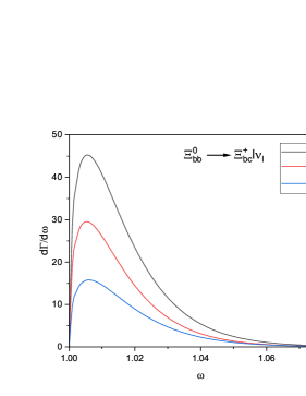
Figure 2: Differential decay rates for $\Xi_{bb}^{0}\rightarrow\Xi_{bc}^{+}l\bar{\nu}_{l}$ transition

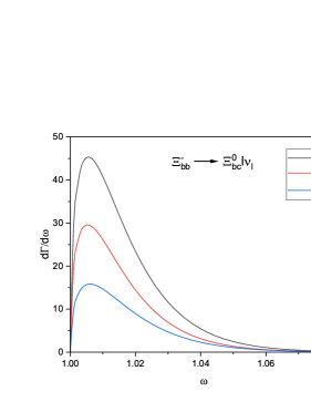
Figure 3: Differential decay rates for $\Xi_{bb}^{-}\rightarrow\Xi_{bc}^{0}l\bar{\nu}_{l}$ transition

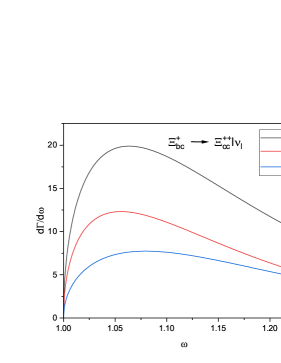
Figure 4: Differential decay rates for $\Xi_{bc}^{+}\rightarrow\Xi_{cc}^{++}l\bar{\nu}_{l}$ transition

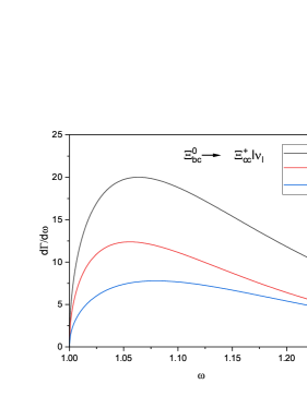
Figure 5: Differential decay rates for $\Xi_{bc}^{0}\rightarrow\Xi_{cc}^{+}l\bar{\nu}_{l}$ transition

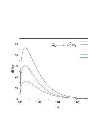
Figure 6: Differential decay rates for $\Omega_{bb}^{-}\rightarrow\Omega_{bc}^{0}l\bar{\nu}_{l}$ transition

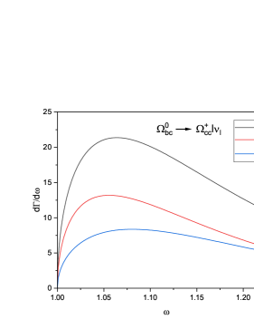
Figure 7: Differential decay rates for $\Omega_{bc}^{0}\rightarrow\Omega_{cc}^{+}l\bar{\nu}_{l}$ transition

$$Br=\Gamma\times\tau$$ (25)

The branching ratio of doubly heavy baryons can be calculated using Eqn. (25) where, $\tau$ is the lifetime of the initial baryon.

5 Results and discussions

We have calculated the ground state masses of all the doubly heavy baryons using the parameters shown in Table 2. The calculated masses of ground state doubly heavy baryons are listed in Table 3. The mass difference between the up quark and down quark have been neglected in all other theoretical predictions shown in Table 3. In the present work, we have considered different quark masses for up and down quarks as, $m_{u}$ = 0.330 GeV and $m_{d}$ = 0.350 GeV (see Table 2). Our calculated masses of doubly heavy baryons are in agreement with the values obtained in Ref. [45]. The values obtained in Ref. [21] are smaller than our calculated masses.

As shown in Table 5, the magnetic moments of doubly heavy baryons are almost matched with other models. The magnetic moment of $\Xi^{0*}_{bb}$ predicted by the Ref. [38] has a negative value while all other theoretical approaches predicted including ours have positive values. The transition magnetic moments of doubly heavy baryons are listed in Table 6. As indicated in Table 6, we can see the good agreement of a computed transition magnetic moments with other predictions except the Ref.[35] which has relatively lower values.

Comparing the radiative decay width with other models, we found that different approaches lead to different results as shown in Table 7. We can see that the radiative decay width is relatively large for $\Xi_{cc}^{++*}\rightarrow\Xi_{cc}^{++}\gamma$ and $\Xi_{cc}^{+*}\rightarrow\Xi_{cc}^{+}\gamma$ in the relativistic three quark model [41] while comparing with others. Our computed radiative decay width for $\Omega_{bb}^{-*}\rightarrow\Omega_{bb}^{-}\gamma$ transition is relatively lower than all other predictions.

Table 8: The semileptonic decay width of doubly heavy baryons $\Gamma$ in $10^{-14}$ GeV

Decay	Our	[45]	[19]	[48]	[44]	[46]	[51]	[49]
$\Xi_{bb}^{0}\rightarrow\Xi_{bc}^{+}l\bar{\nu}_{l}$	1.0526	3.26	1.75	0.98	0.8	0.49	1.92	3.30
$\Xi_{bb}^{-}\rightarrow\Xi_{bc}^{0}l\bar{\nu}_{l}$	1.0539							3.30
$\Xi_{bc}^{+}\rightarrow\Xi_{cc}^{++}l\bar{\nu}_{l}$	4.1456	4.59	3.08	4.39	2.1	3.01	2.57	4.50
$\Xi_{bc}^{0}\rightarrow\Xi_{cc}^{+}l\bar{\nu}_{l}$	4.1589							4.50
$\Omega_{bb}^{-}\rightarrow\Omega_{bc}^{0}l\bar{\nu}_{l}$	1.0828	3.40	1.03	1.87	0.86	0.99	2.14	3.69
$\Omega_{bc}^{0}\rightarrow\Omega_{cc}^{+}l\bar{\nu}_{l}$	4.3336	4.95	3.32	4.7	1.88	3.28	2.59	3.94

To calculate the semileptonic decay rate, we have considered $m_{bb}$ = 2$m_{b}$ = 9.9 GeV and for $bc\rightarrow cc$ transition, $m_{cc}$ = 2$m_{c}$ = 3.1 GeV in the Eqn. (19). We have considered the size parameter $\Lambda_{B}$ = 2.5 GeV [46, 47]. The calculated decay rates of the baryons are listed and compared with other models in Table 8. The present results for the semileptonic decay width of doubly heavy baryons are close to the results predicted by the Ref.[48]. The predicted result of semileptonic decay for $\Xi_{bc}^{+}\rightarrow\Xi_{cc}^{+}+l\bar{\nu}_{l}$ by the Ref.[48] and Ref.[45] are in accordance with the present computed result. It is found that the present computed decay width for $\Xi_{bb}^{0}\rightarrow\Xi_{bc}^{+}l\bar{\nu}_{l}$ transition is lower compared to Ref.[45] and Ref.[49].

The total differential decay rate ($\frac{d\Gamma}{d\omega}$) can be written as a summation of transverse differential decay rate ($\frac{d\Gamma_{T}}{d\omega}$) and longitudinal decay rate ($\frac{d\Gamma_{L}}{d\omega}$) as indicated in Eqn.(22). It is found that the contribution from the transverse decay ($\Gamma_{T}$) is relatively higher compared to the longitudinal decay ($\Gamma_{L}$) as shown in Table 9. We can see that almost $60\%$ of contributions come from $\Gamma_{T}$ while $40\%$ of the contribution comes from $\Gamma_{L}$.

The behaviour of the predicted differential decay rate for semileptonic decay of doubly heavy baryons with $\omega$ are shown in Figure 2 to Figure 7. The peak value of differential decay rate ($\frac{d\Gamma}{d\omega}$) for $\Xi_{bb}$ and $\Omega_{bb}$ baryons is found at $\omega\approx 1.01$ while the peak value for $\Xi_{bc}$ and $\Omega_{bc}$ baryons is found at $\omega\approx 1.06$. The $\frac{d\Gamma}{d\omega}$ of $\Xi_{bb}$ and $\Omega_{bb}$ baryons gets saturated around $\omega\approx 1.06$ while $\Xi_{bc}$ and $\Omega_{bc}$ baryons are at peak value for $\omega\approx 1.06$.

Table 9: The transverse $\Gamma_{T}$ and longitudinal $\Gamma_{L}$ contributions to the width in $10^{-14}$ GeV

Decay	Our	Our	[48]	[48]
	$\Gamma_{T}$	$\Gamma_{L}$	$\Gamma_{T}$	$\Gamma_{L}$
$\Xi_{bb}^{0}\rightarrow\Xi_{bc}^{+}l\bar{\nu}_{l}$	0.65936	0.392697	0.55	0.42
$\Xi_{bb}^{-}\rightarrow\Xi_{bc}^{0}l\bar{\nu}_{l}$	0.660456	0.39347
$\Xi_{bc}^{+}\rightarrow\Xi_{cc}^{++}l\bar{\nu}_{l}$	2.43789	1.70766	1.32	1.75
$\Xi_{bc}^{0}\rightarrow\Xi_{cc}^{+}l\bar{\nu}_{l}$	2.44532	1.71356
$\Omega_{bb}^{-}\rightarrow\Omega_{bc}^{0}l\bar{\nu}_{l}$	0.677688	0.404076	0.58	0.45
$\Omega_{bc}^{0}\rightarrow\Omega_{cc}^{+}l\bar{\nu}_{l}$	2.5431	1.79055	1.4	1.91

Table 10: Obtained values of $\omega_{max}$ for $b\rightarrow c$ transitions

Transition	our	[19]
$\Xi_{bb}^{0}\rightarrow\Xi_{bc}^{+}l\bar{\nu}_{l}$	1.0817	1.07
$\Xi_{bb}^{-}\rightarrow\Xi_{bc}^{0}l\bar{\nu}_{l}$	1.08154
$\Xi_{bc}^{+}\rightarrow\Xi_{cc}^{++}l\bar{\nu}_{l}$	1.2437	1.22
$\Xi_{bc}^{0}\rightarrow\Xi_{cc}^{+}l\bar{\nu}_{l}$	1.24278
$\Omega_{bb}^{-}\rightarrow\Omega_{bc}^{0}l\bar{\nu}_{l}$	1.0798	1.07
$\Omega_{bc}^{0}\rightarrow\Omega_{cc}^{+}l\bar{\nu}_{l}$	1.2329	1.20

The lifetimes of baryons have been studied in Ref. [52, 53, 54, 55]. We have considered $\tau_{\Xi_{bb}^{0}}$ = 0.52$\times 10^{-12}$ s, $\tau_{\Xi_{bb}^{-}}$ = 0.53 $\times 10^{-12}$ s, $\tau_{\Xi_{bc}^{+}}$ = 0.24$\times 10^{-12}$ s, $\tau_{\Xi_{bc}^{0}}$ = 0.22$\times 10^{-12}$ s, $\tau_{\Omega_{bb}^{-}}$ = 0.53 $\times 10^{-12}$ s, $\tau_{\Omega_{bc}^{0}}$ = 0.18$\times 10^{-12}$ s as given in the Ref.[52]. We have calculated the branching ratios using the life time of doubly heavy baryons predicted by the Ref.[52]. While comparing our results for branching ratio with other theoretical predictions, we have computed branching ratio from their predicted decay width in corresponding model and life time mentioned in the Ref.[52]. The computed branching ratio for the $\Omega_{bc}^{0}\rightarrow\Omega_{cc}^{+}l\bar{\nu}_{l}$ semileptonic decay is 1.11$\%$ which is in agreement with the Ref.[49].

Table 11: Branching Ratio in ($\%$), calculated for all models using lifetimes given in Ref. [52].

Transition	Our	[45]	[19]	[48]	[44]	[46]	[51]	[49]
$\Xi_{bb}^{0}\rightarrow\Xi_{bc}^{+}l\bar{\nu}_{l}$	0.8312	1.2877	1.3826	1.489	0.632	0.7426	1.5169	2.6071
$\Xi_{bb}^{-}\rightarrow\Xi_{bc}^{0}l\bar{\nu}_{l}$	0.8486
$\Xi_{bc}^{+}\rightarrow\Xi_{cc}^{++}l\bar{\nu}_{l}$	1.5116	0.8386	1.6007	1.1231	0.7657	1.0975	0.9371	1.6408
$\Xi_{bc}^{0}\rightarrow\Xi_{cc}^{+}l\bar{\nu}_{l}$	1.3901
$\Omega_{bb}^{-}\rightarrow\Omega_{bc}^{0}l\bar{\nu}_{l}$	0.8719	1.3689	1.5058	0.8294	0.6925	0.7972	1.7232	2.9713
$\Omega_{bc}^{0}\rightarrow\Omega_{cc}^{+}l\bar{\nu}_{l}$	1.1185	0.6782	1.2853	0.9079	0.5141	0.8969	0.7083	1.0775

6 Conclusions

The ground state masses are calculated using Hypercentral Constituent Quark Model(hCQM). The magnetic moments of doubly heavy baryons are computed using the spin-flavour wave functions of the constituent quarks and their effective masses within the baryon. We have calculated the radiative M1 decay width from the obtained transition magnetic moment for $\frac{3}{2}^{+}\rightarrow\frac{1}{2}^{+}$ transition. The semileptonic decay rates for doubly heavy baryons are calculated after obtaining the Isgur-wise function. Also, the transverse and longitudinal components of the decay widths are calculated.

References

- [1] C. Patrignani et al. (Particle Data Group), Chin. Phys. C 40(10), 100001 (2016).
- [2] P. A. Zyla et al. (Particle Data Group), Prog. Theor. Exp. Phys. 2020, 083C01 (2020).
- [3] R. L. Workman et al. Review of particle physics. Prog. Theor. Exp. Phys.2022, 083C01 (2022).
- [4] M. Mattson et al.(SELEX Collaboration), Phys. Rev. Lett. 89, 112001 (2002).
- [5] A. Ocherashvili et al. (SELEX Collaboration), Phys. Lett. B 628, 18 (2005).
- [6] R. Aaij et al. (LHCb Collaboration), Phys. Rev. Lett. 119, 112001 (2017).
- [7] R. Aaij et al. (LHCb Collaboration), Phys. Rev. Lett. 121, 162002 (2018).
- [8] R. Aaij et al. (LHCb Collaboration), JHEP 10, 124 (2019).
- [9] R. Aaij et al. (LHCb collaboration), Chin. Phys. C 44, 022001 (2020).
- [10] R. Aaij et al. (LHCb collaboration), JHEP 02, 049 (2020).
- [11] R. Aaij et al. (LHCb Collaboration), JHEP 11, 095 (2020).
- [12] R. Aaij et al. (LHCb Collaboration), Chin. Phys. C 45, 093002(2021).
- [13] R. Aaij et al. (LHCb collaboration), Sci. China Phys. Mech. Astron. 63, 221062 (2020).
- [14] R. Aaij et al. (LHCb collaboration), JHEP 12, 107 (2021).
- [15] R. Aaij et al. (LHCb collaboration), Sci. China Phys. Mech. Astron. 64, 101062 (2021).
- [16] W. Roberts and Muslema Pervin, arXiv:0711.2492 [nucl-th] (2008).
- [17] M. Farhadi et al. Eur. Phys. J. A 59, 171 (2023).
- [18] D. Ebert, R. N. Faustov, V. O. Galkin and A. P. Martynenko, Phys. Rev. D 70, 014018 (2004).
- [19] Z. Ghalenovi, C.P. Shen, M. Moazzen Sorkhi, Phys. Lett. B 834, 137405 (2022).
- [20] Z. X. Zhao, Eur. Phys. J. C 78, 756 (2018).
- [21] M. S. Tousi, K. Azizi, Phys. Rev. D, 109(5), 054005(2024).
- [22] Y. J. Shi, W. Wang, Z. X. Zhao, and U. G. Meiner, Eur. Phys. J. C 80, 398 (2020).
- [23] Q. X. Yu and X. H. Guo, Nucl. Phys. B 947, 114727 (2019).
- [24] Z. S. Brown, W. Detmold, S. Meinel, K. Orginos, Phys. Rev. D 90(9), 094507 (2014).
- [25] S. S. Gershtein, V. V. Kiselev, A. K. Likhoded, and A. I. Onishchenko, Phys. Rev. D 62, 054021 (2000).
- [26] M. Padmanath, arXiv:1905.10168 (2019).
- [27] N. Isgur, M.B. Wise, Phys. Lett. B 237, 527 (1990).
- [28] K. Thakkar, Z. Shah, A. K. Rai and P. C. Vinodkumar, Nuclear Physics A 965, 57-73 (2017).
- [29] K. Thakkar, Eur. Phys. J. C 80(10), 926 (2020).
- [30] H Garcilazo, J Vijande and A Valcarce, et al., J. Phys. G: Nucl. and Part. Phys. 34, 961 (2007).
- [31] E. Santopinto, F. Lachello, M.M. Giannini, Eur. Phys. J. A 1, 307 (1998).
- [32] M. Ferraris, M.M. Giannini, M. Pizzo, E. Santopinto, L. Tiator, Phys. Lett. B 364, 231 (1995).
- [33] K. Thakkar, B. Patel, A. Majethiya, P.C. Vinodkumar, Pramana J. Phys. 77, 1053 (2011).
- [34] A. Majethiya, B. Patel, P. C. Vinodkumar, Eur. Phys. J. A, 42, 213 (2009); [Erratum]: Eur. Phys. J. A 38,307 (2008).
- [35] A. Bernotas, V. Šimonis, Phys. Rev. D 87, 074016 (2013).
- [36] G. Wagner, A. J. Buchmann, A. Faessler, J. Phys. G 26, 267 (2000).
- [37] A. N. Gadaria, N. R. Soni, J. N. Pandya, DAE Symp. Nucl. Phys. 61, 698699 (2016).
- [38] Z. Shah, A. Kakadiya, K. Gandhi, A. K. Rai, Universe, 7, 337 (2021).
- [39] A. Hazra, S. Rakshit, R. Dhir, Phys. Rev. D 104, 053002 (2021).
- [40] V. Šimonis, arXiv:1803.01809 (2018).
- [41] T. Branz, A. Faessler, T. Gutsche, M. A. Ivanov, J. G. Körner, V. E. Lyubovitskij, and B. Oexl, Phys. Rev. D 81, 114036 (2010).
- [42] Q. F. Lü, K. L. Wang, L. Y. Xiao and X. H. Zhong, Phys. Rev. D 96, 114006 (2017).
- [43] C. Albertus, E. Hernández and J. Nieves, Phys. Rev. D 71, 014012 (2005).
- [44] A. Faessler et. el, Phys. Rev. D 80, 034025 (2009).
- [45] D. Ebert, R. N. Faustov et al. Phys. Atom. Nuclei 68, 784-807 (2005).
- [46] S. Rahmani and H. hassanabadi, Eur. Phys. J. C 80, 312 (2020).
- [47] M. A. Ivanov, V. E. Lyubovitskij, J. G. Körner and P. Kroll, Phys. Rev. D 56, 348 (1997).
- [48] Z. Ghalenovi, M. Moazzen Sorkhi, Chin. Phys. C 47, 033105(2023).
- [49] W. Wang, F. S. Yu, Z.X. Zhao, Eur. Phys. J. C 77, 781 (2017).
- [50] M. Karliner, J. L. Rosner, Phys. Rev. D 90, 094007 (2014).
- [51] C. Albertus, E. Hernández, J. Nieves and J. M. Verde-Velasco, Eur. Phys. J. A 32, 183 (2007), [Erratum]: Eur. Phys. J. A 36, 119 (2008).
- [52] A. V. Berezhnoy, A. K. Likhoded, A. V. Luchinsky, Phys. Rev. D 98, 113004 (2018).
- [53] V. V. Kiselev and A. K. Likhoded, Phys. Usp. 45, 455 (2002) [Usp. Fiz. Nauk 172, 497 (2002)].
- [54] A. K. Likhoded, A.V.Luchinsky, Physics of Atomic Nuclei, Vol. 81, 6 (2018).
- [55] H. Cheng and F. Xu, Phys. Rev. D 99, 073006 (2019).