A Reinforcement Learning based Motion Planner for Quadrotor Autonomous Flight in Dense Environment
Abstract
Quadrotor motion planning is critical for autonomous flight in complex environments, such as rescue operations. Traditional methods often employ trajectory generation optimization and passive time allocation strategies, which can limit the exploitation of the quadrotor’s dynamic capabilities and introduce delays and inaccuracies. To address these challenges, we propose a novel motion planning framework that integrates visibility path searching and reinforcement learning (RL) motion generation. Our method constructs collision-free paths using heuristic search and visibility graphs, which are then refined by an RL policy to generate low-level motion commands. We validate our approach in simulated indoor environments, demonstrating better performance than traditional methods in terms of time span.
I Introduction
Quadrotors are extensively used in a variety of applications, including rescue operations, fire and electricity inspection, and package delivery. Achieving autonomous flight in complex environments necessitates effective motion planning, which is crucial for ensuring safe and efficient navigation. State-of-the-art motion planning algorithms for quadrotors primarily focus on generating collision-free and dynamic feasible trajectories, subsequently optimizing them to achieve smoothness and aggressiveness. Time allocation plays a pivotal role in the trajectory generation process, as suboptimal time allocation can lead to inefficient trajectories and underutilization of the quadrotor’s dynamic capabilities.
However, traditional methods predominantly employ passive time allocation strategies, which may not fully exploit the quadrotor’s dynamic capabilities within its constraints. Additionally, the trajectories generated by these optimizers must be tracked by a controller, introducing delays, increased computational overhead, and discrepancies between the optimized and actual flight trajectories.
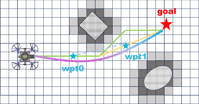
To address these challenges, we propose a novel reinforcement learning (RL)-based motion planner for quadrotor autonomous flight in dense environments. Our approach aims to maximize the utilization of the quadrotor’s dynamic capabilities while relying only on a low-level controller. Our method employs a path searching algorithm based on heuristic search and visibility graphs, which constructs a collision-free, minimum-length path in a discrete grid space. This initial path is then converted into waypoints, serving as control points for the RL motion generator. The policy network generates low-level control commands based on observations of the quadrotor’s state, control points, and environmental information, optimizing the quadrotor’s motion (Fig. 1). These low-level commands are directly sent to the quadrotor’s controller, ensuring motion within predefined limits of velocity, acceleration, and attitude.
Compared to existing motion planners, our method deviates from conventional trajectory generation and optimization frameworks by directly generating motion using an RL policy. It can handle discrete paths that may not satisfy kinodynamic and non-holonomic constraints, producing aggressive, collision-free motion within the specified dynamic constraints. We demonstrate the effectiveness and robustness of our method through extensive simulations and discuss its potential transferability to real-world quadrotor platforms, that will do later. Our key contributions are summarized as follows:
-
(1)
This letter propose a robust and efficient RL-based method that integrates visibility path searching and RL motion generation, directly generating feasible and aggressive motions from the policy.
-
(2)
We incorporate heuristic search and visibility graph concepts to develop a grid map-based pathfinding algorithm that generates collision-free, minimum-length paths.
-
(3)
We investigate optimal RL environment settings and obstacle information configurations for planning in dense environments, enabling motion generation from any initial state.
-
(4)
We provide extensive simulation evaluations of the proposed method and discuss its potential transferability to real-world quadrotor platforms.
II Related Work
II-A Optimal Control Methods
Quadrotor motion planning has been extensively studied, with optimal control-based trajectory optimization methods prevailing as the predominant approach. These methods focus on generating smooth, dynamically feasible, and collision-free trajectories by solving optimization tasks modeled as optimal control problems. The pioneering approach is the minimum-snap trajectory generation[1] in differential flatness outputs, representing the trajectory as a polynomial and using gradient descent to iteratively modify the time segments. Several works propose two-stage solving methods where trajectory generation occurs in the second stage [2, 3, 4, 5, 6, 7]. For instance, [2] introduces a safe flight corridor composed of convex polyhedra, providing constraints for optimization. The method in [3] combines sampling-based and gradient optimization methods to achieve smooth, feasible, and safe trajectories. [4] utilizes B-spline for kinodynamic path searching, adopting an elastic optimization method to refine trajectories. The Euclidean Signed Distance Field (ESDF) map is employed in [8] to obtain collision potentials and in [5] to find a path in the velocity field, improving time allocation. [6] proposes a comprehensive pipeline for quadrotor motion planning, including kinodynamic path searching, B-spline trajectory generation, time allocation, and nonuniform B-spline optimization based on ESDF. Subsequent works [9, 10] introduce topological path and risk-aware yaw planning. Given the computational intensity of constructing ESDF, [11] proposes an ESDF-free gradient-based planner. However, [12] demonstrates a method to generate ESDF rapidly. These methods effectively generate smooth, safe, and feasible trajectories. However, they may be conservative regarding the quadrotor’s dynamic capabilities due to passive time allocation. In contrast, [13] and [14] focuses on spatial-temporal deformation, which aligns with our approach by considering both geometric and temporal planning concurrently.
II-B RL based Methods
RL-based methods have gained significant traction in quadrotor motion planning due to their capability to optimize non-convex and discontinuous objectives, which traditional approaches often struggle to handle effectively. In [15], the authors propose an imitation learning (IL)-based teacher-student pipeline that directly maps noisy sensory depth images to polynomial trajectories. While IL is quite efficient, its scalability is limited by the need for expert data collection. [16] employs a topological path searching algorithm to generate guiding paths, followed by RL to generate control commands. This two-stage method performs well in selected scenarios, outperforming some traditional methods. [17] extracts features from depth images and uses a teacher-student IL framework similar to [15]. Furthermore, it generates control commands directly and includes a perception reward to guide yaw planning. In [18, 19], Song investigates the strengths and limitations of optimal control and RL, proposing that RL is advantageous as it can optimize better objectives that may be infeasible for optimal control methods to address.
Current RL-based methods often incorporate high-order dynamic parameters like body rate and attitude into their observations to compose trajectories or low-level control commands. Despite their advanced techniques, these methods frequently rely on imitation learning (IL) with expert knowledge or are tested in fixed environments, limiting their generalization and transferability to unknown environments, and failing to enable autonomous flight in new scenarios. Our RL approach also uses high-order dynamic parameters as observations but focuses on simplifying the learning tasks for RL. Instead of expecting RL to handle the entire path searching process, we use RL as an optimizer to refine motion and control points, similar to B-spline optimization schemes. This strategy allows for more efficient learning and better adaptation to complex environments.
III System Overview
III-A Quadrotor dynamics
We model the quadrotor as a linear system with translational and rotational dynamics decoupled. The dynamics equations are
| (1) |
| (2) |
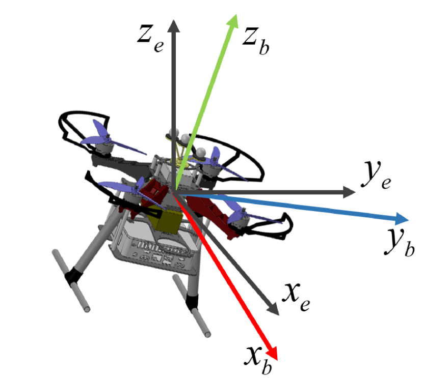
where is position in earth frame, is velocity, is rotation matrix from body frame to earth frame, is z axis in body frame, is thrust of each rotor, is mass, is drag coefficient, is diagonal inertia matrix, is angular velocity in body frame, and is gyroscopic torque and torque by thrusts respectively. We use Euler angles to represent rotation and set a limit on roll and pitch angles to avoid singularity.
The control allocation matrix that can be used to get relation between thrusts and torques is given by
| (3) |
where denotes rotor’s torque coefficient, and represents the distance from the center of mass to the rotor center. The complete state of the quadrotor is defined as , with indicating roll, pitch and yaw angle.The control input is given by . We use simpson’s rule to do numerical integration for state update.
III-B Visibility RL Planning Structure
The proposed planning framework is illustrated in Fig. 2. The planning process operates in two stages. First, the Visibility Path Searching algorithm constructs a reference path from the start to the goal, ensuring obstacle avoidance and path length minimization. This reference path is discretized into waypoints based on the current position and the distance to the next obstacle corner (Section IV). Second, the RL Motion Generation method produces control commands to optimize the quadrotor’s motion. These commands enable the quadrotor to follow the waypoints within a certain tolerance, determining the required proximity to waypoints and strategies for obstacle avoidance in continuous space, as presented in Section V.
IV Visibility Path Searching
Our pathfinding algorithm integrates the A*, Jump Point Search (JPS)[20], and Visibility Graph methods. We inherit the heuristic function and the open and closed list architecture from the A* algorithm but use a different cost function. Elements of the JPS method are incorporated to reduce the number of nodes in the open list, minimizing computational costs associated with sorting these nodes. Additionally, we leverage the optimal distance characteristics of the Visibility Graph method without constructing complex polygon edges and vertices.
The proposed strategy facilitates omnidirectional movement through obstacle corner detection and visibility checks, rather than restricting movement to increments of in 2D plane. This approach is implemented by selecting obstacle corners in the Corner function and assessing voxel visibility in the VisibleCheck function. Consequently, this method reduces the computational and memory overhead typically required for accessing each vertex and edge of the voxels. The detailed algorithm is presented in Algorithm 1.
IV-A Obstacle Corner Search
We define an obstacle corner as a voxel with only one occupied neighbor, indicating its location at the edge of an obstacle. In the context of the Visibility Graph, the optimal path from the start to the goal point traverses vertices that represent the corners of obstacles. Therefore, obstacle corners Corner, including the start and goal points, are exclusively utilized as elements in the open list. This approach reduces the number of nodes in the open list and decreases sorting costs, similar to JPS, while maintaining the optimal path characteristics of the Visibility Graph.
The cost of a obstacle corner using EuclideanCost is defined as
| (4) |
IV-B Visibility Expansion
When a new obstacle corner is detected, the Bresenham algorithm[21] is employed to perform a visibility check using VisibleCheck, determining whether the corner is visible from the current node. Only corners confirmed to be visible are considered as child nodes and candidates for the open list, ensuring that a connected path of vertices via line segments is traced from start to goal. We adopt an expansion method from Hybrid A*[22] in RandomVisibleCheck to verify the existence of a collision-free path between the current node and the goal along a line segment. The invocation frequency of this function increases as the distance to the goal decreases.
V RL Motion Generation
V-A Policy Framework
We construct the control points optimizing and motion generating problem in a reinforcement learning (RL) framework using Markov Decision Process (MDP) defined by tuple . The quadrotor agent begins in a state that is selected from state space distribution . In this setting, the agent interacts with the environment by sampled action from a random policy . After that, the state of the agent will be updated from to by the transition probability , and a reward will be given to the agent. Detailed configuration of the state space, action space, and reward function will be discussed in the following sections.
V-A1 Observation and action space
The observation space contains three main parts: state of the quadrotor, waypoints information and ESDF based obstacle details. Specifically, we denote the state vector as
| (5) |
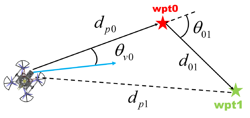
And the observation vector is derived from the state vector, incorporating some elements directly from it, including . We convert other state elements to low level features, which would be more generalized and easier for policy training. For example, waypoints position combined with absolute position of the quadrotor are used to calculate relative position of the quadrotor to target waypoints. We also add a normalized vector representing the direction from current position to the next waypoint in body frame, which is used to guide the limit of field of view (FOV) of depth camera with direction of in body frame. The detailed obstacle information is composed by the ESDF map of the environment, which will be discussed in the following section.
The action produced by RL policy is , is the collective thrust by all motors and is the desired body rate, which has been proved to perform well in learning-based quadrotor control and planning tasks. Although this control command is usually used in drone racing tasks due to its low latency and high frequency, it also takes a significant gap between simulation and real world. Despite this drawback, this approach can result in better smoothness in acceleration and velocity, which will be beneficial in energy saving and safety.
V-A2 Reward function
According to paper RL vs OC, RL outperforms Optimal Control (OC) in terms of optimizing a better objective that OC may not be able to solve. From this perspective, we design a reward function that explicitly represents better active time allocation, collision avoidance, and smoothness in motion based on RL vs OC. The reward function is defined as
| (6) |
where is the customized progress reward, is punishment for state violation, is the reward for arriving at one waypoint, is the punishment for collision, and is the penalty for large angular velocity.
Specifically, the progress reward is defined as
| (7) |
We normalize the progress reward within interval and subsequently introduce a negative term , thereby imposing a time penalty which facilities time allocation and maximized the utilization of the quadrotor’s dynamic capabilities.
For state violation penalty , we impose limits on acceleration and velocity to ensure dynamic smoothness and safety. Additionally, attitude limits are set to prevent overly aggressive maneuvers and avoid singularities.
| (8) |
Specifically, represents the number of elements from the set that exceed their prescribed limits.
V-B Training methodology
We create a training environment based on OpenAI gym, providing an interface for creating a customized environment. At the beginning of each episode, the velocity, body rate, orientation, waypoints and obstacles are randomly initialized following a predefined probabilistic pattern which is shown in Fig.3, while the position if fixed at the center of the map.
V-B1 Quadrotor state initialization
Since we are using only two waypoints for the whole navigation, we make the first waypoint totally randomized with only the distance from quadrotor position to the waypoint withing a certain range.
| (9) |
where is a randomly generated unit vector, and and define the waypoint distance range. The second waypoint is given by
The second waypoint is set to within a certain distance and angle from the first waypoint and the line from quadrotor position to the first waypoint.
| (10) |
where is a unit vector such that , with being the angle between and . must lie within the waypoint distance range and ensure that the distance between the quadrotor and the second waypoint exceeds .
Concerning velocity, constraints are applied to ensure the velocity direction does not deviate significantly, expressed as , as the path searching algorithm is expected not to produce waypoints that are in a direction completely opposite to the current velocity. We also set constraints on the orientation of the quadrotor as
| (11) |
V-B2 Obstacles setting
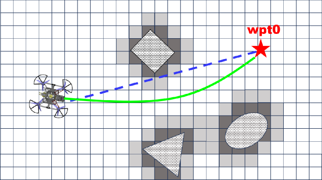
In our framework, RL is expected to generate motions based on collision-free waypoints obtained after path searching. These waypoints might still be close to or intersect with obstacles after sampling. Therefore, we only need to place obstacles on or near the lines from the quadrotor to the waypoints, rather than creating a maze-like environment. Additionally, it is essential to ensure a feasible path exists between the quadrotor position and the waypoints (see Fig. 4).
V-B3 Obstacle avoidance
Although the guided waypoints from path searching can avoid obstacles in voxel level, the quadrotor still needs to avoid obstacles in continuous space, which is achieved adding related observation and reward in RL framework.
We truncate ESDF map into TSDF map due to two reasons: first, we expect RL framework as a local motion generator to be more efficient in terms of active time allocation and collision avoidance; second, the ideal range of depth camera is limited, which is more suitable for TSDF map.
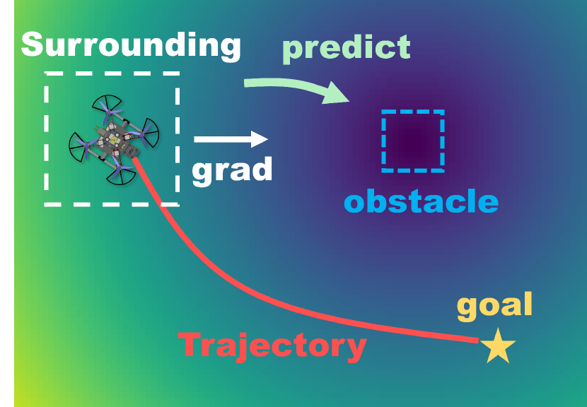
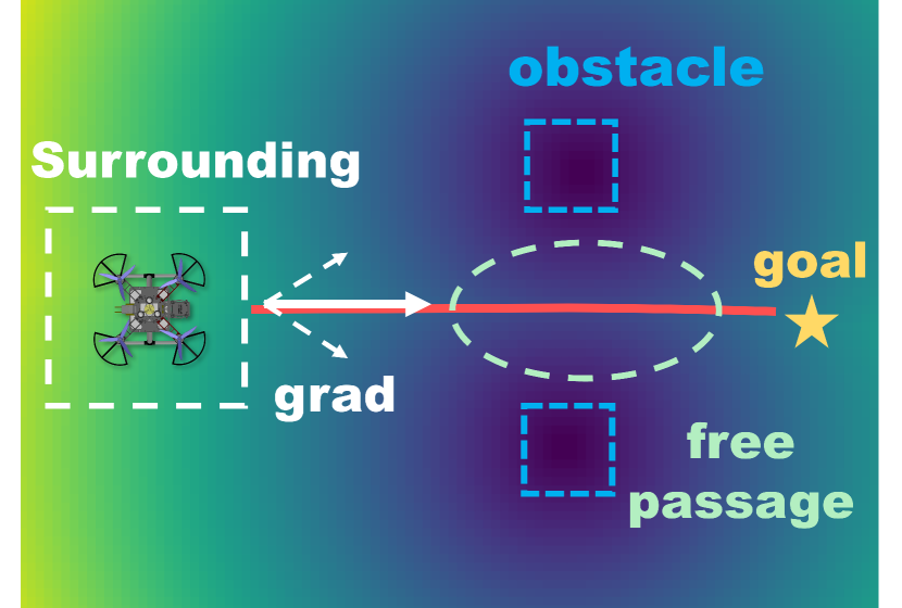
While SDF maps can address some motion planning problems, they often require the entire map or significant portions. In an RL framework, excessive information can hinder generalization. Using SDF data can aid in obstacle avoidance but is not comprehensive for all scenarios, as illustrated in Fig. 5. A more efficient method for quadrotor environmental understanding is necessary.
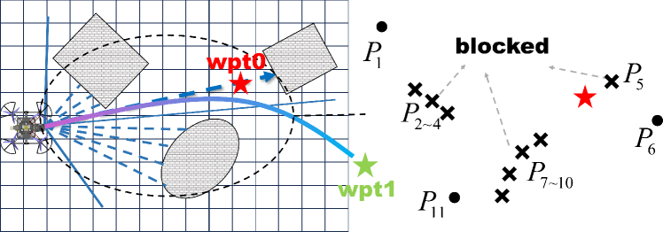
To address these issues and better align with our objectives, we propose a method named ray guiding, which provides understanding the basic distribution of obstacles by ray sampling and accurate velocity limitations by ray searching. To comprehensively assess the surrounding obstacles, we sample ray castings from the quadrotor’s position to the first waypoint at irregular angles centered around the waypoint direction (see Fig. 6). The end positions of each beam are used in the observation space. While this method offers a broad understanding of the space around the quadrotor, its accuracy is affected by the interval of rays, the sensing range, and the map’s resolution.
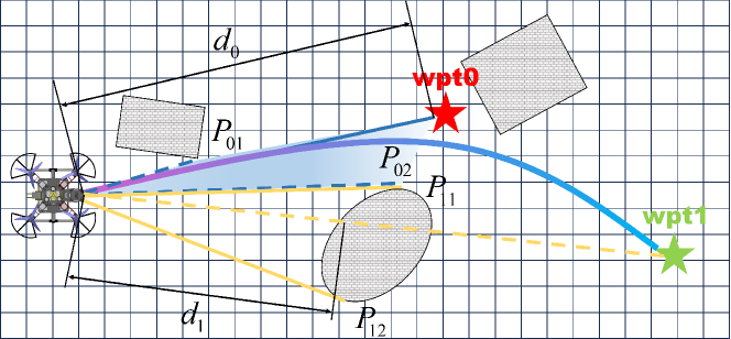
Since ray sampling provides a rough obstacle distribution, we further refine the observation using ray search. The core idea is to define safe regions in the velocity field that guide the quadrotor’s velocity towards the waypoint safely, enhancing both efficiency and reliability (see in Fig. 7). We first cast rays from the quadrotor towards the waypoints, spreading them in a cone shape to detect obstacles’ edges and free space within a certain range. If the direct ray to the waypoint is blocked, we search for a transition point from obstacle to free space. If unblocked, we identify the obstacle edges. The final ray search observation for a waypoint is given as .
V-C Sim to real transfer
Transferring a policy trained in a customized environment to simulation and then to a real-world platform is challenging due to factors like inaccurate modeling of quadrotor dynamics, system delays, low-level controller errors, and action oscillations introducing high-order system complexities. We implement strategies to mitigate these issues.
We first train the policy in a customized Gym-based environment before transferring it to Gazebo simulation with PX4 firmware and then testing it on our real quadrotor platform (IMP250) with a Pixhawk 6c flight controller, without fine-tuning. We meticulously identified the Iris drone and our quadrotor models, achieving a relatively accurate representation. To ensure compatibility with low-level control, we utilize the PX4 multicopter rate controller and mixer to compute thrust and torques from the desired body rate and collective thrust outputs of the RL policy.
Additionally, we apply domain randomization during RL training to enhance policy robustness and prevent overfitting, compensating for numerical integration errors and modeling discrepancies between simulation and reality. We randomized the quadrotor’s physical properties, including mass, inertia, and thrust mapping, and ignored battery voltage drop and motor heating effects due to short flight times.
VI Results
VI-A Training details
The policy is trained using the Proximal Policy Optimization (PPO)[23] algorithm in Stable-Baselines3[24], which has demonstrated strong performance in various continuous control tasks, including drone racing. We train two separate models for scenarios with and without obstacles to streamline training and improve efficiency. This approach also mitigates the issue of forgetting, which we encountered when sequentially training a single model first on obstacle-free and then on obstacle-present cases. The decision to use a specific model depends on the values from the ESDF map and the camera’s ideal range.
| Variable | Value | Variable | Value | |
| iris | [kg] | 0.535 | [-] | 0.12 |
| [] | 0.029 | [m] | 0.13 | |
| [] | 0.029 | [m] | 0.2 | |
| [] | 0.055 | [m] | 0.22 | |
| [-] | 0.6 | [] | 3.14 | |
| [-] | 0.15 | [] | 1.31 | |
| RL | [] | 6.0 | [] | 3.0 |
| [-] | 2.0 | [-] | 5.0 | |
| [-] | 10 | [-] | -350 | |
| [-] | 0.01 | [-] | 1.5 | |
| [m] | 2.5 | [m] | 0.5 | |
| [s] | 0.02 | [m] | 0.3 | |
| [m] | 0.15 | [-] | 0.99 | |
| batch size [-] | 64 | learning rate [-] | 0.0003 |
The quadrotor’s physical properties and the RL algorithm’s hyperparameters are listed in Table I. We utilize the Iris quadrotor model from the PX4 firmware, adjusting its mass to 0.535 kg and the torque constant to 0.12 for our purposes. Following previous research, we employ Runge-Kutta 4th order numerical integration to update the quadrotor’s state, excluding aerodynamic drag during training due to its insignificance for the current .
All policies are trained on a desktop computer equipped with an NVIDIA RTX 4090 GPU and an Intel i9-13900K CPU.
VI-B Analysis and Comparison
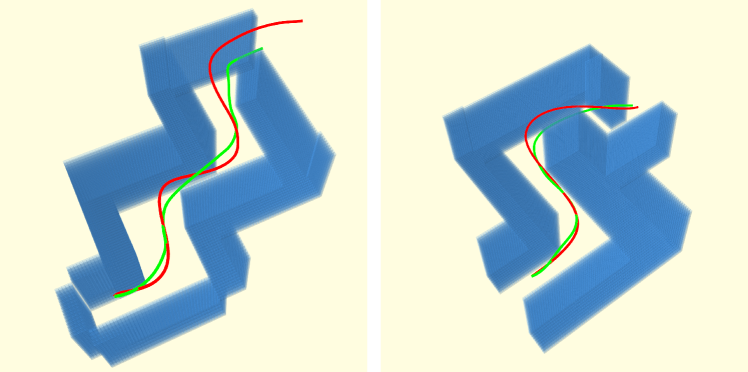
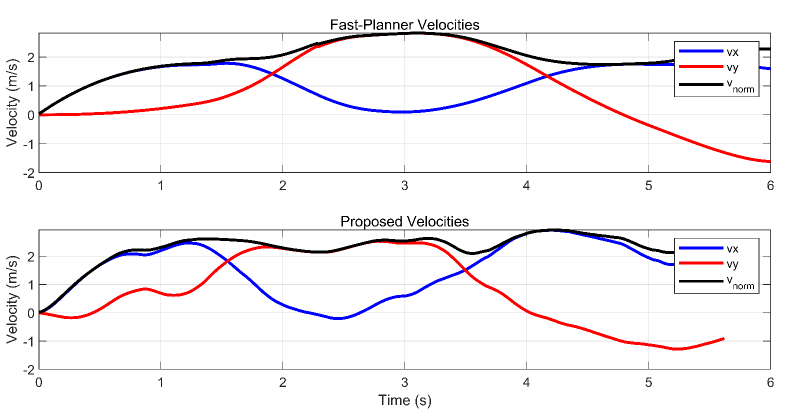
We compare our method with Fast-Planner [6] in terms of time to reach the same waypoint, energy consumption (integral of jerk), and computation time, with plans to include additional baselines in future work. Fast-Planner and our method employ ESDF for path searching and motion or trajectory generation. To ensure fairness, we remove control disturbances and initialize both methods from the same state. Our evaluation is conducted in two densely obstructed indoor scenarios, using identical models to assess and compare performance against Fast-Planner. The maximum velocity and acceleration for baseline methods are set to be and , respectively. For collision detection in the configuration space, the baseline methods use the same inflated obstacle size as ours, . Additionally, we impose stricter limits on z-axis position (), sensing horizon (), and searching horizon () to align with our method. Other parameters are set to default values.
| Time Span () | Energy () | |
|---|---|---|
| (1)Fast-Planner | 8.26 | 176.86 |
| (1)Ours | 5.80 | 935.88 |
| (2)Fast-Planner | 6.03 | 44.36 |
| (2)Ours | 4.78 | 576.76 |
To date, our method has demonstrated better performance in terms of time span, although the energy consumption remains much higher than that of Fast-Planner due to the aggressive control commands generated by the RL policy. Additionally, our method is less risk-aware compared to Fast-Planner, as it does not incorporate active perception, highlighting a potential direction for future work.
VII Conclusion
In this letter, we propose a novel quadrotor motion planning framework that integrates path searching and motion generation using visibility-based methods and reinforcement learning. Our approach employs visibility path searching to generate safe waypoints with minimal path length, which are further optimized by an RL policy to produce low-level motion commands. We validate our method in two simulated indoor environments and compare it with Fast-Planner, demonstrating better performance in terms of time span.
Future work will focus on optimizing the RL policy to reduce energy consumption and enhance risk awareness through active yaw planning. We also plan to extend our method to real-world scenarios and evaluate its performance on a real quadrotor platform soon. Additionally, we aim to explore the potential of our approach in dynamic environments.
Acknowledgment
The authors would like to Yunlong Song for suggestions and discussions on RL policy training and sim to real transfer, Jia Xu and Zeshuai Chen for discussion on control and real-world platform.
References
- [1] D. Mellinger and V. Kumar, “Minimum snap trajectory generation and control for quadrotors,” in 2011 IEEE International Conference on Robotics and Automation, 2011, pp. 2520–2525.
- [2] S. Liu, M. Watterson, K. Mohta, K. Sun, S. Bhattacharya, C. J. Taylor, and V. Kumar, “Planning dynamically feasible trajectories for quadrotors using safe flight corridors in 3-d complex environments,” IEEE Robotics and Automation Letters, vol. 2, no. 3, pp. 1688–1695, 2017.
- [3] F. Gao, Y. Lin, and S. Shen, “Gradient-based online safe trajectory generation for quadrotor flight in complex environments,” in 2017 IEEE/RSJ International Conference on Intelligent Robots and Systems (IROS), 2017, pp. 3681–3688.
- [4] W. Ding, W. Gao, K. Wang, and S. Shen, “An efficient b-spline-based kinodynamic replanning framework for quadrotors,” IEEE Transactions on Robotics, vol. 35, no. 6, pp. 1287–1306, 2019.
- [5] F. Gao, W. Wu, Y. Lin, and S. Shen, “Online safe trajectory generation for quadrotors using fast marching method and bernstein basis polynomial,” in 2018 IEEE International Conference on Robotics and Automation (ICRA), 2018, pp. 344–351.
- [6] B. Zhou, F. Gao, L. Wang, C. Liu, and S. Shen, “Robust and efficient quadrotor trajectory generation for fast autonomous flight,” IEEE Robotics and Automation Letters, vol. 4, no. 4, pp. 3529–3536, 2019.
- [7] J. Tordesillas, B. T. Lopez, M. Everett, and J. P. How, “Faster: Fast and safe trajectory planner for navigation in unknown environments,” IEEE Transactions on Robotics, vol. 38, no. 2, pp. 922–938, 2022.
- [8] H. Oleynikova, M. Burri, Z. Taylor, J. Nieto, R. Siegwart, and E. Galceran, “Continuous-time trajectory optimization for online uav replanning,” in 2016 IEEE/RSJ International Conference on Intelligent Robots and Systems (IROS), 2016, pp. 5332–5339.
- [9] B. Zhou, F. Gao, J. Pan, and S. Shen, “Robust real-time uav replanning using guided gradient-based optimization and topological paths,” in 2020 IEEE International Conference on Robotics and Automation (ICRA), 2020, pp. 1208–1214.
- [10] B. Zhou, J. Pan, F. Gao, and S. Shen, “Raptor: Robust and perception-aware trajectory replanning for quadrotor fast flight,” IEEE Transactions on Robotics, vol. 37, no. 6, pp. 1992–2009, 2021.
- [11] X. Zhou, Z. Wang, H. Ye, C. Xu, and F. Gao, “Ego-planner: An esdf-free gradient-based local planner for quadrotors,” IEEE Robotics and Automation Letters, vol. 6, no. 2, pp. 478–485, 2021.
- [12] A. Millane, H. Oleynikova, E. Wirbel, R. Steiner, V. Ramasamy, D. Tingdahl, and R. Siegwart, “nvblox: Gpu-accelerated incremental signed distance field mapping,” 2024. [Online]. Available: https://arxiv.org/abs/2311.00626
- [13] F. Gao, W. Wu, J. Pan, B. Zhou, and S. Shen, “Optimal time allocation for quadrotor trajectory generation,” in 2018 IEEE/RSJ International Conference on Intelligent Robots and Systems (IROS), 2018, pp. 4715–4722.
- [14] Z. Wang, X. Zhou, C. Xu, and F. Gao, “Geometrically constrained trajectory optimization for multicopters,” IEEE Transactions on Robotics, vol. 38, no. 5, pp. 3259–3278, 2022.
- [15] A. Loquercio, E. Kaufmann, R. Ranftl, M. Müller, V. Koltun, and D. Scaramuzza, “Learning high-speed flight in the wild,” Science Robotics, vol. 6, no. 59, p. eabg5810, 2021. [Online]. Available: https://www.science.org/doi/abs/10.1126/scirobotics.abg5810
- [16] R. Penicka, Y. Song, E. Kaufmann, and D. Scaramuzza, “Learning minimum-time flight in cluttered environments,” IEEE Robotics and Automation Letters, vol. 7, no. 3, pp. 7209–7216, 2022.
- [17] Y. Song, K. Shi, R. Penicka, and D. Scaramuzza, “Learning perception-aware agile flight in cluttered environments,” in 2023 IEEE International Conference on Robotics and Automation (ICRA), 2023, pp. 1989–1995.
- [18] Y. Song, A. Romero, M. Müller, V. Koltun, and D. Scaramuzza, “Reaching the limit in autonomous racing: Optimal control versus reinforcement learning,” Science Robotics, vol. 8, no. 82, p. eadg1462, 2023. [Online]. Available: https://www.science.org/doi/abs/10.1126/scirobotics.adg1462
- [19] Y. Song, M. Steinweg, E. Kaufmann, and D. Scaramuzza, “Autonomous drone racing with deep reinforcement learning,” in 2021 IEEE/RSJ International Conference on Intelligent Robots and Systems (IROS), 2021, pp. 1205–1212.
- [20] D. Harabor and A. Grastien, “Online graph pruning for pathfinding on grid maps,” Proceedings of the AAAI Conference on Artificial Intelligence, vol. 25, no. 1, pp. 1114–1119, Aug. 2011. [Online]. Available: https://ojs.aaai.org/index.php/AAAI/article/view/7994
- [21] J. E. Bresenham, “Algorithm for computer control of a digital plotter,” IBM Systems Journal, vol. 4, no. 1, pp. 25–30, 1965.
- [22] D. Dolgov, S. Thrun, M. Montemerlo, and J. Diebel, “Path planning for autonomous vehicles in unknown semi-structured environments,” The International Journal of Robotics Research, vol. 29, no. 5, pp. 485–501, 2010. [Online]. Available: https://doi.org/10.1177/0278364909359210
- [23] J. Schulman, F. Wolski, P. Dhariwal, A. Radford, and O. Klimov, “Proximal policy optimization algorithms,” 2017. [Online]. Available: https://arxiv.org/abs/1707.06347
- [24] A. Raffin, A. Hill, A. Gleave, A. Kanervisto, M. Ernestus, and N. Dormann, “Stable-baselines3: Reliable reinforcement learning implementations,” Journal of Machine Learning Research, vol. 22, no. 268, pp. 1–8, 2021. [Online]. Available: http://jmlr.org/papers/v22/20-1364.html