Jumping on the bandwagon and off the Titanic: an experimental study of turnout in two-tier voting

Abstract

We experimentally study voter turnout in two-tier elections when the electorate consists of multiple groups, such as states. Votes are aggregated within the groups by the winner-take-all rule or the proportional rule, and the group-level decisions are combined to determine the winner. We observe that, compared with the theoretical prediction, turnout is significantly lower in the minority camp (the Titanic effect) and significantly higher in the majority camp (the behavioral bandwagon effect), and these effects are stronger under the proportional rule than under the winner-take-all rule. As a result, the distribution of voter welfare becomes more unequal than theoretically predicted, and this welfare effect is stronger under the proportional rule than under the winner-take-all rule.

1 Introduction

Studies of endogenous voter turnout have focused on direct voting in which individuals’ votes are aggregated directly to make a social decision. However, there are also cases where social decision-making takes the form of two-tier voting: votes are aggregated separately in distinct groups, and the group-level decisions are combined to make a final decision. For instance, in presidential elections in the United States, the electoral votes of each state is divided between the candidates based on the statewide popular vote, and the candidate with the most electoral votes is chosen for president. As another example, in elections for national parliaments, states or prefectures elect representatives, who then collectively make policy decisions through legislative voting.

Participation decision in two-tier voting is more complex than in direct voting, since a voter must consider both his influence on his group’s decision and the group’s influence on the social decision. Given the complexity of the problem, actual voter behavior may differ significantly from theoretical predictions. Moreover, turnout may depend on the electoral rules that specify how votes are aggregated within groups. The rules then affect voter welfare not only directly by converting a configuration of votes into a social decision, but also indirectly by affecting the incentives of voters to participate. To understand how two-tier voting systems work, we extend the standard costly voting model to a multi-group setup, compare voter turnout in theory and experiment, and draw welfare implications for alternative electoral rules.

We construct a model of two-candidate election with three groups of voters (e.g., states), each having a voting weight (e.g., electoral votes) proportional to population. Each voter decides whether to vote for her preferred candidate or abstain, by comparing the expected benefits and costs of voting. Each group’s weight is then allocated to the candidates according to some aggregation rule based on their vote shares within the group. A candidate wins if he obtains a majority of the total weights across the three groups. We consider two alternative rules used widely in real politics. Under the winner-take-all rule (WTA), the whole weight of a group goes to the candidate who receives a majority of votes in the group. Under the proportional rule (PR), each group’s weight is divided between the candidates proportionally to their vote shares in the group.

In our experiment, we simplify the decision problems to reduce the complexity of considerations necessary for subjects to play the voting game with a multi-group structure. Precisely, among the three voter groups, one group (“human group”) consists of human subjects while the other two groups (“computer groups”) consist of automated voters programmed to play the equilibrium strategies.

We find two prominent behavioral patterns, the behavioral bandwagon effect and the Titanic effect, and that the magnitudes of these effects differ under WTA and PR. The behavioral bandwagon effect refers to the case where the observed turnout rate is higher than the theoretical prediction among voters in the majority camp (i.e., those voters in the human group who support the candidate preferred by the majority of voters in the group). On the other hand, the Titanic effect refers to the case where the observed turnout rate is lower than the theoretical prediction among voters in the minority camp. The behavioral bandwagon and Titanic effects are observed under both WTA and PR, but the magnitude is more substantial under PR. Moreover, these effects appear discontinuously around the fifty-fifty split in the support rate between the two candidates, suggesting that being in the majority or minority itself affects the participation decision. Consequently, majority turnout tends to exceed minority turnout, which is consistent with a number of previous experimental studies, yet contrasts with the underdog effect observed by Levine and Palfrey (2007).

Our theoretical model enables us to simulate the impact of these behavioral effects on voter welfare. The experimental observation that turnout increases among majority voters and decreases among minority voters leads to higher (resp. lower) voting costs and larger (smaller) expected benefits from the victory for the majority (minority) candidate, compared with the theoretical prediction. According to our model, the impact of expected benefits dominates the effect of voting costs. As a result, the majority’s welfare increases and the minority’s welfare decreases from the theoretical levels. We also find that these welfare effects are stronger under PR than under WTA. Therefore, the distribution of voter welfare becomes more unequal than theoretically predicted, and this welfare effect is stronger under PR than under WTA. These observations point to the importance of taking behavioral effects into account in normative evaluation of two-tier election rules.

The multi-group framework also allows us to distinguish the majority-minority relationships at the group level and the social level. We call a voter local majority if she prefers the candidate supported by a majority of her group, and global majority if she prefers the candidate supported by a majority of the whole electorate. Our analysis of the experimental data reveals that being local majority or minority has stronger effects on voter turnout than being global majority or minority does.

1.1 Related Literature

To our knowledge, this paper is the first to experimentally study endogenous turnout in two-tier voting. Welfare properties of two-tier voting rules have been studied extensively (e.g. Barberà and Jackson, 2006; Koriyama et al., 2013; Kurz, Maaser, and Napel, 2017; Kikuchi and Koriyama, 2023). However, little attention has been paid as to how those rules affect voters’ turnout incentives. In particular, Kikuchi and Koriyama (2023) compares welfare between the winner-take-all rule and the proportional rule, assuming that all voters vote. The present paper complements that study by extending the model to allow voters to abstain.

There are experimental studies that compare turnout under different electoral rules, focusing on the case of direct voting. These studies compare different power sharing rules (mostly majority rule and proportional representation), assuming that the resulting power shares of parties enter directly into voters’ payoffs. Schram and Sonnemans (1996) compares voter turnout between majority rule and proportional representation to observe higher turnout under the majority rule, as predicted by the theory. Herrera, Morelli, and Palfrey (2014) compares turnout between the two rules according to the minority’s size. Their data supports the theoretical predictions. Kartal (2015) compares minority representation as well as voter turnout between the two rules. She observes that proportional representation does not improve the representation of a small minority compared with the theoretical prediction. The main departure of the present paper from the approach of these studies is to define electoral rules as part of a two-tier voting system, whose ultimate outcome is a social decision (e.g., the winner of a presidential election or the result of a legislative vote), not the power shares of parties per se.

Kartal (2015) reports an effect similar to the Titanic effect observed in our experiment. In her experiment, the turnout rate of minority voters under proportional representation was significantly lower than theoretically predicted. As a possible explanation, she suggests that minority voters may have been discouraged from voting, due to an election threshold resulting from a discrete nature of proportional representation. The proportional rule in our experiment has no such election threshold and yet exhibits a similar effect on minority turnout.

The behavioral bandwagon and Titanic effects are closely related to the bandwagon effect, which refers to the phenomenon that information that a candidate is more (less) likely to win stimulates (discourages) participation from the supporters of the candidate. The bandwagon effect is not consistent with the underdog effect predicted by standard voting models such as Palfrey and Rosenthal (1983, 1985) and observed experimentally by Levine and Palfrey (2007). But it has been observed in many of the previous experiments, including Faravelli, Kalayci, and Pimienta (2020) who reexamined Levine and Palfrey’s (2007) results through Amazon’s Mechanical Turk with larger electorate size and real-effort costs of voting.

Großer and Schram (2010) experimentally shows that majority voters turn out more often than minority voters, and the release of opinion polls further increases this difference. Agranov et al. (2018) develops a novel experimental design which elicits subjects’ beliefs about the election outcome, and shows that the subjects are more likely to vote when they believe that their preferred candidate is more likely to win. Morton and Ou (2015) surveys the psychological and political-economy literature on the mental process behind the bandwagon effect. They also examine experimentally the condition under which other-regarding and non-other-regarding bandwagon behaviors are likely to appear, respectively. Grillo (2017) provides a theoretical explanation for the bandwagon effect in terms of risk aversion of voters.

2 Model

2.1 Two-tier election

Two candidates, $I=A,B$, compete in an election. The electorate consists of three groups, $g=1,2,3$. Let $n_{g}$ denote the population of group $g$. Each group $g$ has a voting weight (e.g., electoral votes) equal to its population $n_{g}$. The election proceeds as follows. Each voter casts one vote for a candidate or abstains. The weight of each group is then allocated to the candidates based on their vote shares in the group, according to some aggregation rule. A candidate wins the election if she receives a majority of the total weights across the three groups.

Each voter in group $g$ independently prefers candidate $A$ with probability $p_{g}\in[0,1]$ and candidate $B$ with probability $1-p_{g}$. The probability $p_{g}$ represents the support rate for candidate $A$ in group $g$. The support rate may vary across the groups, reflecting group-specific bias. Each voter obtains a benefit of $\beta>0$ if her preferred candidate wins. Voting incurs a cost $c_{i}$ for voter $i$. We assume that the voting cost is independent across voters and uniformly distributed on an interval $[0,\bar{c}]$, which is common knowledge among voters. The realized preferences and costs are private information: voter $i$ knows her preferred candidate and cost $c_{i}$, but not those of the other voters.

This situation constitutes a voting game in which voters in all groups simultaneously choose whether to vote for their preferred candidate or abstain, after observing their own voting cost and preferred candidate. Voter $i$ chooses her action to maximize her expected payoff, defined as the benefit $\beta$ weighted by the probability that her preferred candidate wins, minus the cost ($c_{i}$ or 0 depending on whether she votes or abstains).

We consider two alternative rules that specify how the weight of a group is allocated to the candidates based on the groupwise voting result. Under the winner-take-all rule (WTA), each group allocates the whole weight to the candidate who receives a majority of votes in the group. Under the proportional rule (PR), each group divides the weight between the two candidates proportionally to their vote shares in the group. For simplicity, we focus on the case where all groups employ the same rule.

We call a specification of the group sizes $(n_{1},n_{2},n_{3})$ and the candidate support rates $(p_{1},p_{2},p_{3})$ a voting configuration. We also call a pair of a voting configuration and a rule (WTA or PR) a voting situation.

2.2 Equilibrium

Our theoretical prediction for this voting game is based on the concept of quasi-symmetric equilibrium. In equilibrium, each voter maximizes her expected payoff given the other voters’ strategies. By quasi-symmetric, we mean that all voters in the same group play the same strategy. It is easy to check that any quasi-symmetric equilibrium consists of cutpoint strategies. A cutpoint strategy for voter $i$ is a pair of cutpoints $\hat{c}_{i}=(\hat{c}_{i,A},\hat{c}_{i,B})\in[0,\bar{c}]^{2}$ such that, conditional on preferred candidate $I$, she votes for $I$ if $c_{i}\leq\hat{c}_{i,I}$ and abstains if $c_{i}>\hat{c}_{i,I}$. In a quasi-symmetric equilibrium, voters in the same group have the same cutpoints; hence the equilibrium is a profile $\hat{c}=(\hat{c}_{g})_{g=1,2,3}$ in which $\hat{c}_{g}=(\hat{c}_{g,A},\hat{c}_{g,B})$ represents (with a slight abuse of notation) the strategy for voters in group $g$. Given the cutpoint strategy profile $\hat{c}$, the probability that a supporter of candidate $I$ in group $g$ votes equals ${t}_{g,I}=\frac{\hat{c}_{g,I}}{\bar{c}}$, which approximately equals the turnout rate among $I$-supporters in group $g$.

An equilibrium condition can be obtained as a set of equations involving the probability that a voter is pivotal, meaning that her vote overturns the election outcome. Consider a voter $i$ in group $g$ who prefers candidate $I$, and let $\pi_{g,I}(\hat{c})$ be the probability that the voter is pivotal, which is a function of the cutpoint strategy profile $\hat{c}=(\hat{c}_{g})_{g=1,2,3}$. The voter’s expected benefit of voting is $\beta\pi_{g,I}(\hat{c})$, so she votes if $c_{i}\leq\beta\pi_{g,I}(\hat{c})$ and abstains if $c_{i}>\beta\pi_{g,I}(\hat{c})$. Therefore, voter $i$’s choice of the cutpoint $\hat{c}_{g,I}$ is a best response to the profile $\hat{c}$ if and only if

$$\hat{c}_{g,I}=\beta\pi_{g,I}(\hat{c}).$$ (1)

The strategy profile $\hat{c}$ is an equilibrium if and only if equation (1) holds for all groups $g=1,2,3$ and candidates $I=A,B$. The two rules, WTA and PR, induce different pivot probability functions $\pi_{g,I}(\cdot)$ and, therefore, different equilibria.

3 Experimental Design

3.1 Human and computer groups

We conducted an experiment on the voting game described in the previous section. To reduce the complexity of the decision problem for the subjects, we set up only group 1 as a human group consisting of subjects, while the remaining groups 2 and 3 as computer groups consisting of automated voters programmed to play the equilibrium strategies.

3.2 Decision problem

Figure 1 is an image of the screen shown to the subjects in each voting situation. Two candidates are labeled Orange and Green. Voters in the three groups independently become a supporter of either candidate, according to the probabilities $(p_{1},p_{2},p_{3})$. The preferences are private information: each subject knows her own preferred candidate, but does not know the preferences of the other voters (human or computer). Each subject observes the population sizes ($n_{1},n_{2},n_{3}$), the aggregation rule (WTA or PR), the support rates of the candidates ($p_{1}$) in the human group, and the probabilities of each automated voter in the computer groups to vote for Orange, vote for Green, or abstain, where these probabilities for the computer groups are derived from the equilibrium strategies.

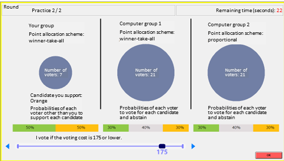
Figure 1: The decision screen

Given this information, each subject chooses a threshold of the cost below which she votes, by moving the slider over the interval displayed on the screen. The subject can choose any integer in the set $S=\{0,1,2,\dots,200\}$.

Once all subjects have made their choice, the voting costs are independently drawn from the uniform distribution over $S$. Each voter votes for her preferred candidate if the cost is within her threshold, and abstains otherwise. The votes are aggregated within each group, and the voting weights are allocated to the candidates according to the pre-specified rule, which determines the winner of the election.

Each subject obtains 1,000 points if her preferred candidate wins. The voting cost is subtracted if she has voted. The screen then displays a summary of the results: the number of votes cast for each candidate, the amount of each group’s voting weight allocated to each candidate, the election winner, the points obtained by the subject, and the subtracted cost.

3.3 Local and global majority

Table 1 shows the 18 voting configurations used in our experiment. Given our setting with three groups of voters, it is useful to define the notions of majority and minority in local and global senses. We say that candidate $A$ is local minority (and candidate $B$ local majority) if $A$ is minority in the human group, i.e., if $p_{1}<0.5$. We say that candidate $A$ is global minority (and candidate $B$ global majority) if $A$ is minority among the entire electorate, i.e., if $\bar{p}<0.5$, where $\bar{p}$ denotes the overall support rate for $A$ among the electorate: $\bar{p}=(p_{1}n_{1}+p_{2}n_{2}+p_{3}n_{3})/(n_{1}+n_{2}+n_{3})$.

Table 1: Voter configurations

Configuration	Category	$n_{1}$	$n_{2}$	$n_{3}$	$p_{1}$	$p_{2}$	$p_{3}$	$\bar{p}$
1	IC	21	21	21	0.5	0.5	0.5	0.5
2	IC	21	21	7	0.5	0.5	0.5	0.5
3	IC	21	21	3	0.5	0.5	0.5	0.5
4	Global	21	21	21	0.5	0.5	0.35	0.45
5	Local	21	21	21	0.1	0.7	0.7	0.5
6	Both	21	21	21	0.35	0.5	0.5	0.45
7	Global	21	21	7	0.5	0.5	0.35	0.48
8	Both	21	21	7	0.48	0.48	0.48	0.48
9	Both	21	21	7	0.45	0.5	0.5	0.48
10	IC	7	7	7	0.5	0.5	0.5	0.5
11	IC	7	21	21	0.5	0.5	0.5	0.5
12	Both	7	21	21	0.15	0.5	0.5	0.45
13	Local	7	21	21	0.1	0.57	0.57	0.5
14	Global	7	7	7	0.5	0.5	0.35	0.45
15	Local	7	7	7	0.1	0.7	0.7	0.5
16	Both	7	7	7	0.35	0.5	0.5	0.45
17	Both	7	21	21	0.48	0.48	0.48	0.48
18	Global	7	21	21	0.5	0.5	0.45	0.48

Our experiment focuses on those voting configurations in which one candidate, say candidate $A$, is weak minority both locally and globally (i.e., $p_{1}\leq 0.5$ and $\bar{p}\leq 0.5$). The 18 voting configurations used in the experiment are classified into four categories, as in Table 2. In category 1, called impartial culture (IC), the two candidates are equally preferred by voters locally and globally, and hence there is no majority or minority candidate (i.e., $p_{1}=\bar{p}=0.5$). Category 2 concerns global asymmetry only (hereafter Global): the two candidates are equally preferred in group 1, but candidate $B$ is more preferred among the whole electorate (i.e., $p_{1}=0.5$ and $\bar{p}<0.5$), implying that candidate $B$ is preferred over candidate $A$ in groups 2 and/or 3. Category 3 concerns the reverse case, local asymmetry only (hereafter Local). Candidate $B$ is more preferred in group 1, but the two candidates are equally preferred among the whole electorate (i.e., $p_{1}<0.5$ and $\bar{p}=0.5$), implying that candidate $A$ is preferred over candidate $B$ in groups 2 and/or 3. Finally, category 4 concerns both local and global asymmetry (hereafter Both): candidate $B$ is preferred over candidate $A$ locally and globally (i.e., $p_{1}<0.5$ and $\bar{p}<0.5$).

Table 2: Categories of voting configurations.

Category	Local support rate	Global support rate
1. Impartial Culture (IC)	$p_{1}=0.5$	$\bar{p}=0.5$
2. Global asymmetry only (Global)	$p_{1}=0.5$	$\bar{p}<0.5$
3. Local asymmetry only (Local)	$p_{1}<0.5$	$\bar{p}=0.5$
4. Both local and global asymmetry (Both)	$p_{1}<0.5$	$\bar{p}<0.5$

3.4 Sessions

We conducted the experiment through 8 sessions, each with 21 human subjects. Each session consists of 36 rounds, with all subjects playing each of the 18 voting configurations exactly once under each of WTA and PR. The voting situations are divided into four blocks specified by the electoral rule (WTA or PR) and the size of the human group (7 or 21). We changed the order of blocks and reversed the order of voting configurations within a block session by session to minimize the order effect (see Table 3).

Table 3: Session summary: order of blocks

Session No.	1,5	2,6	3,7	4,8
1st block	WTA, 21	WTA, 7	PR, 21	PR, 7
2nd	WTA, 7	WTA, 21	PR,7	PR,21
3rd	PR, 21	PR, 7	WTA, 21	WTA, 7
4th	PR, 7	PR, 21	WTA, 7	WTA, 21

One typical session lasted for approximately 130 minutes. At the end of each session, one voting situation per block was randomly selected, and subjects were paid for the sum of points earned in four randomly selected situations. We sent Amazon gift card via email for payment. The average payment was 3,053 JPY (1 point = 1 JPY, 27.9 USD as of June 1st, 2021).

3.5 Logistics

The eight sessions took place in March and June 2021. Our experiment was programmed with the z-Tree Unleashed (Duch, Grossmann, and Lauer, 2020) and ran online through a virtual server in Amazon Elastic Compute Cloud (EC2). Subjects were recruited via the ORSEE (Greiner, 2015) from the campus-wide student subject pool at Osaka University. Thirty-four percent of the participants were female.

Prior to each session, subjects were gathered in a Zoom meeting, where they were identified and anonymized. Instructions were shown by sharing a screen, and read by a text-to-speech software, which served to control time and tone. While the instructions were being read, an experimenter indicated the relevant part of the screen by a pointer. The instruction material was accessible for the subjects anytime during the session via a hyperlink. After playing 36 rounds of voting, the subjects answered the post-experimental questionnaire distributed by Google Forms (See Section 4.3 for the details).

4 Results

4.1 The bandwagon and Titanic effects

Table 4 shows the comparison of turnout rates between equilibrium and experiment. The turnout rate ${t}_{1,I}^{R}$ represents that of a voter in the human group (i.e., group 1) for each candidate $I\in\{A,B\}$ and rule $R\in\{\rm WTA,PR\}$, over the 18 voting configurations used in our experiment.

Table 4: Comparison of turnout rates: equilibrium and experiment.

Config.	Cat.	Equilibrium				Experiment (average)
		$t_{1,A}^{\rm WTA}$	$t_{1,B}^{\rm WTA}$	$t_{1,A}^{\rm PR}$	$t_{1,B}^{\rm PR}$	$\hat{t}_{1,A}^{\rm WTA}$	$\hat{t}_{1,B}^{\rm WTA}$	$\hat{t}_{1,A}^{\rm PR}$	$\hat{t}_{1,B}^{\rm PR}$
1	IC	0.359	0.359	0.391	0.391	0.449	0.473	0.495	0.448
2	IC	0.359	0.359	0.424	0.424	0.471	0.493	0.504	0.462
3	IC	0.359	0.359	0.442	0.442	0.481	0.477	0.489	0.467
4	Global	0.359	0.359	0.367	0.383	0.340	0.486	0.321	0.496
5	Local	0.283	0.144	0.753	0.250	0.071	0.291	0.103	0.457
6	Both	0.368	0.301	0.437	0.333	0.184	0.444	0.218	0.522
7	Global	0.359	0.359	0.417	0.425	0.410	0.440	0.415	0.491
8	Both	0.363	0.353	0.427	0.416	0.340	0.465	0.301	0.471
9	Both	0.368	0.345	0.441	0.405	0.288	0.494	0.314	0.559
10	IC	0.516	0.516	0.553	0.553	0.420	0.532	0.485	0.451
11	IC	0.516	0.516	0.421	0.421	0.410	0.408	0.434	0.375
12	Both	0.585	0.344	0.630	0.301	0.188	0.407	0.113	0.428
13	Local	0.588	0.307	0.737	0.287	0.121	0.309	0.161	0.369
14	Global	0.516	0.516	0.526	0.555	0.329	0.543	0.306	0.489
15	Local	0.538	0.284	1.000	0.354	0.162	0.309	0.195	0.455
16	Both	0.553	0.455	0.629	0.480	0.232	0.530	0.175	0.540
17	Both	0.521	0.508	0.424	0.414	0.322	0.472	0.285	0.392
18	Global	0.516	0.516	0.415	0.422	0.370	0.479	0.362	0.367

We first investigate the effects of being majority or minority on subjects’ participation decisions. We here focus on the voting configurations in the categories where the majority and the minority are well-defined (Global, Local and Both). Figure 2 plots the pairs of theoretical and observed turnout rates in the majority camp ($\bullet$) and the minority camp ($\circ$) in the human group under WTA (left) and PR (right). Each dot represents a voting configuration displaying the turnout rates averaged over all sessions.

We find two prominent behavioral patterns, the behavioral bandwagon effect and the Titanic effect, and that these effects are stronger under PR than WTA. We say that the behavioral bandwagon effect occurs if the observed turnout rate among voters in the majority camp is higher than the theoretical prediction. On the other hand, we say that the Titanic effect occurs if the observed turnout rate among voters in the minority camp is lower than the theoretical prediction. Figure 2 shows that these effects are evident: most black dots lie above the 45-degree line, while most white dots lie below it.

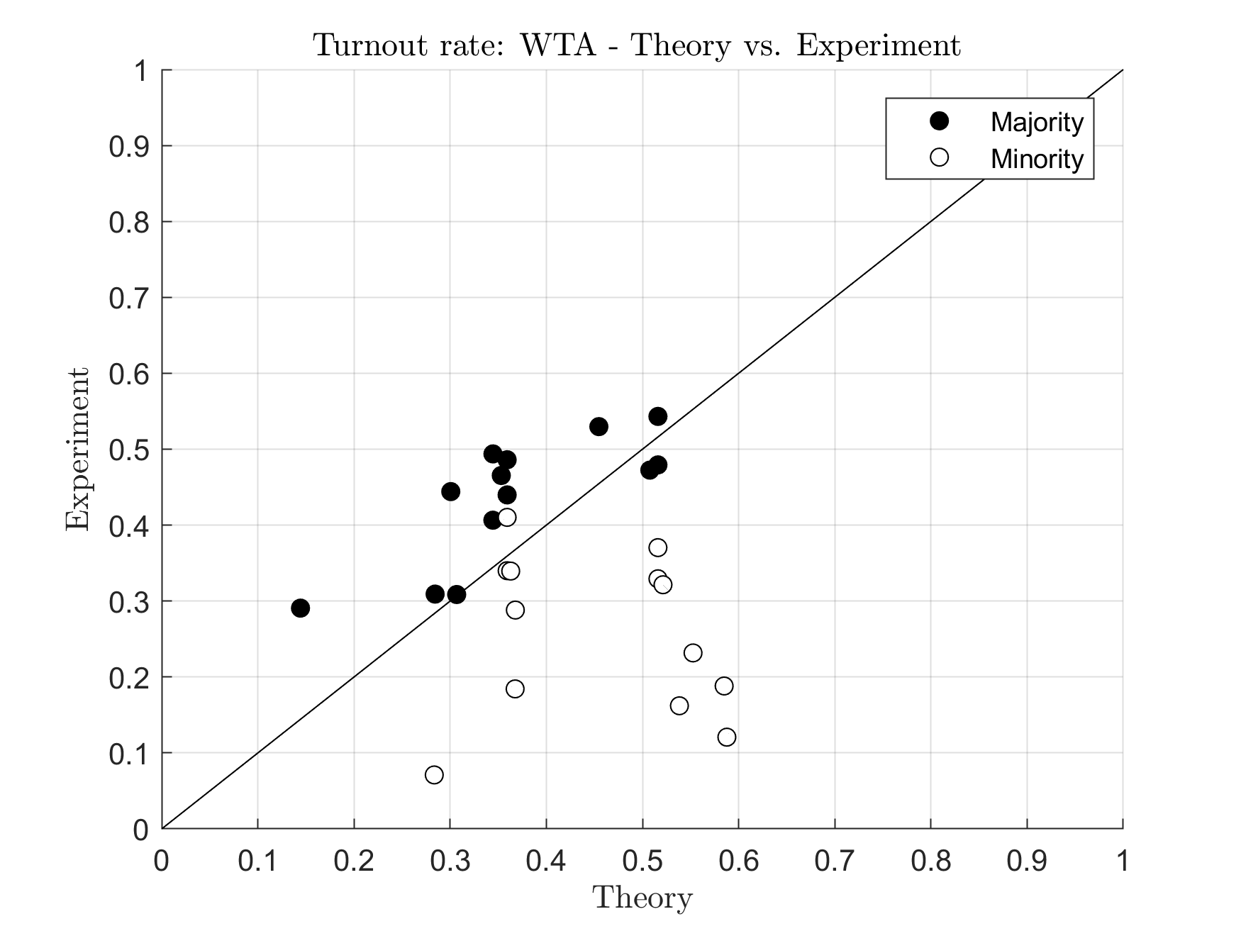
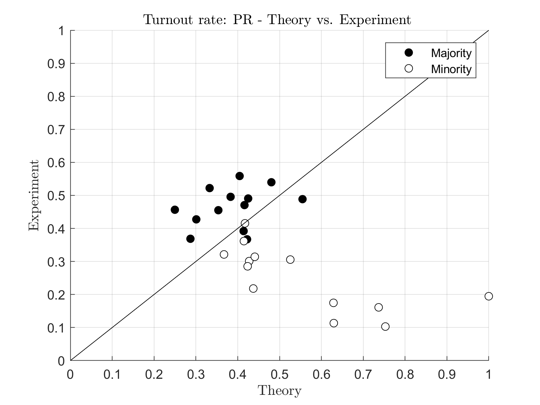
Figure 2: Turnout rate: comparison between theory and experiment.

The non-parametric one-sample Wilcoxon tests statistically confirm the two behavioral effects. Table 5(b) summarizes the test results. For the behavioral bandwagon (resp. Titanic) effect, out of the 13 voting configurations in Global, Local and Both categories the difference between theory and experiment is statistically significant in 4 (10) under WTA and 6 (11) under PR. The Titanic effect appears stronger than the behavioral bandwagon effect, and both effects appear more prominent under PR than WTA.

Table 5: Difference of turnout rates, [Experiment]$-$[Theory].

(a) Panel A: Majority - Behavioral bandwagon effect.

WTA
Global	config. 4	7	14	18
	0.127	0.081	0.027	$-$0.037
Local	config. 5	13	15
	0.146	0.002**	0.025
Both	config. 6	8	9	12	16	17
	0.144	0.112*	0.149**	0.062	0.075**	$-$0.035
PR
Global	config. 4	7	14	18
	0.113	0.066**	$-$0.066	$-$0.055
Local	config. 5	13	15
	0.207***	0.082	0.101**
Both	config. 6	8	9	12	16	17
	0.189***	0.055	0.154***	0.127	0.059**	$-$0.022

(b) Panel B: Minority - Titanic effect.

WTA
Global	config. 4	7	14	18
	$-$0.019	0.051	$-$0.187***	$-$0.146***
Local	config. 5	13	15
	$-$0.212***	$-$0.467***	$-$0.376***
Both	config. 6	8	9	12	16	17
	$-$0.183***	$-$0.023	$-$0.080*	$-$0.397***	$-$0.321***	$-$0.200***
PR
Global	config. 4	7	14	18
	$-$0.046	$-$0.002	$-$0.220***	$-$0.053*
Local	config. 5	13	15
	$-$0.650***	$-$0.576***	$-$0.805***
Both	config. 6	8	9	12	16	17
	$-$0.219***	$-$0.126***	$-$0.127**	$-$0.516***	$-$0.454***	$-$0.138***
***$p<0.01$, **$p<0.05$, *$p<0.1$, Wilcoxon one-sample test.

4.2 Welfare consequences

What are the implications of these behavioral patterns for voter welfare under different electoral rules? To answer this question, we provide a comparison of the expected welfare of the majority and minority voters in each voting configuration based on the experimental data. Observed threshold values are regarded as constituting a sample from a hypothetical mixed strategy played in each voting situation, and the ex-ante expected payoffs are computed assuming that all subjects play the mixed strategy. The behavior of the two computer groups is fixed at the equilibrium strategies, as is done in the experiment.

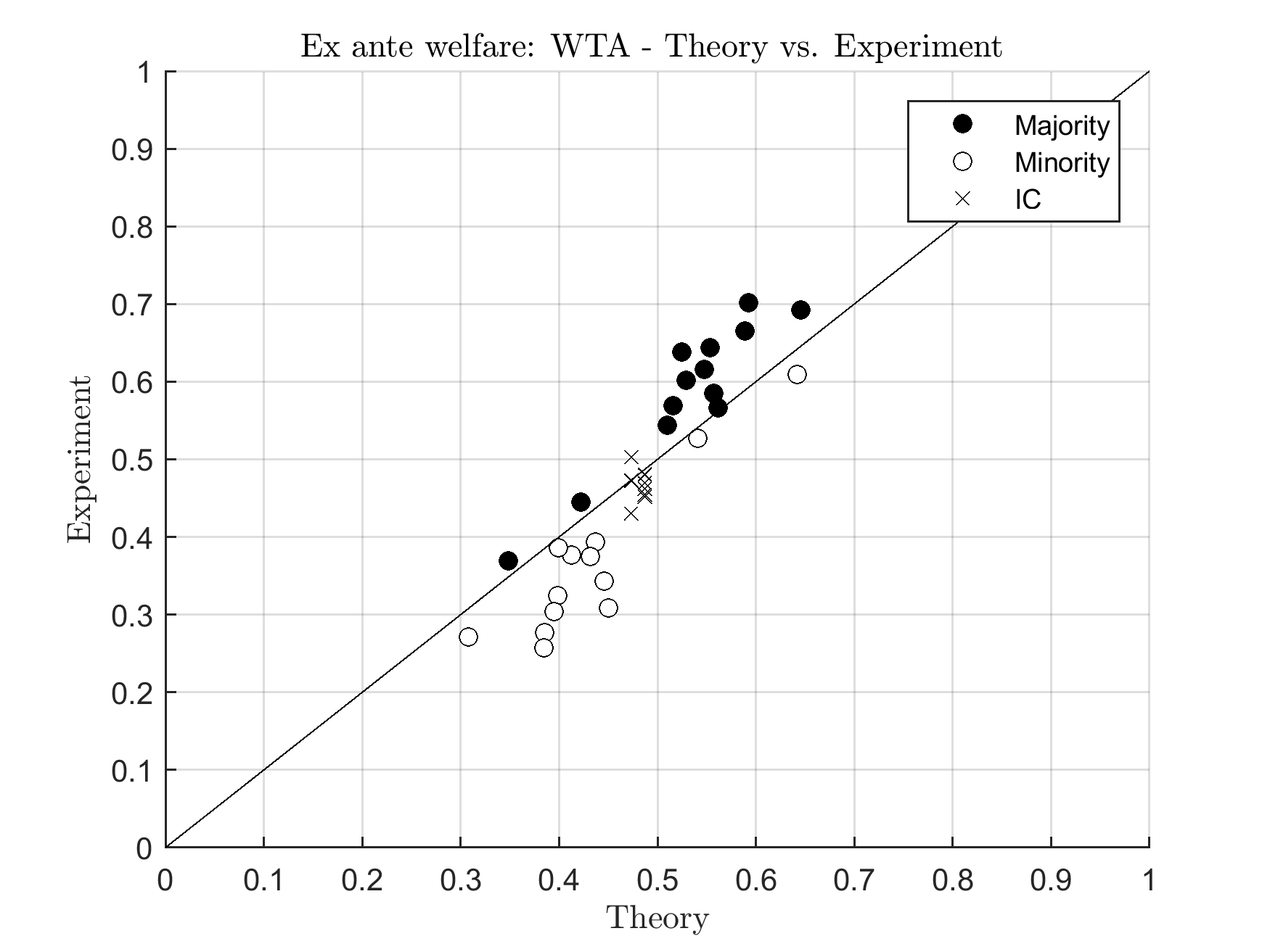
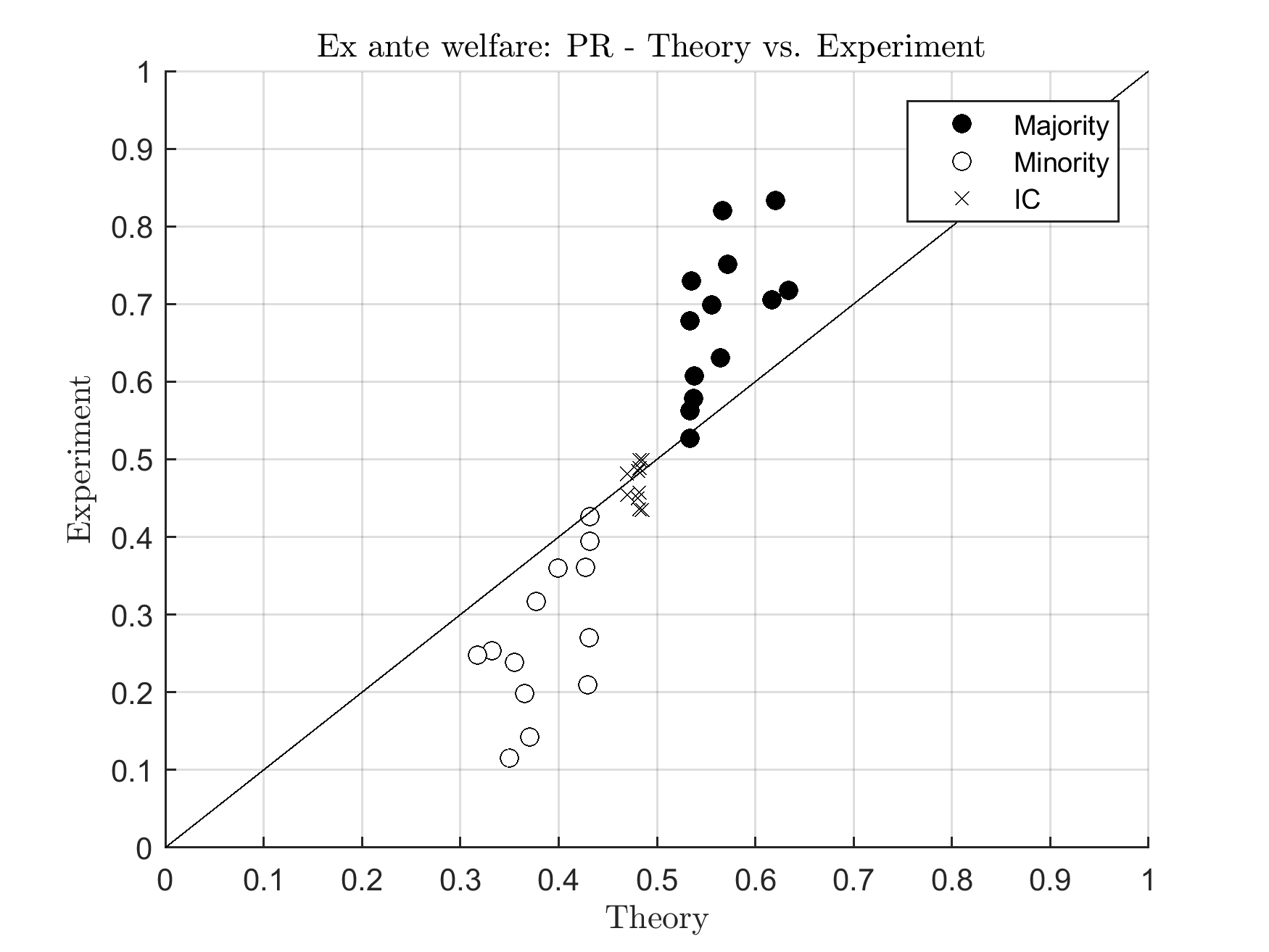
Figure 3: Ex-ante welfare: comparison between the theory and experiment.

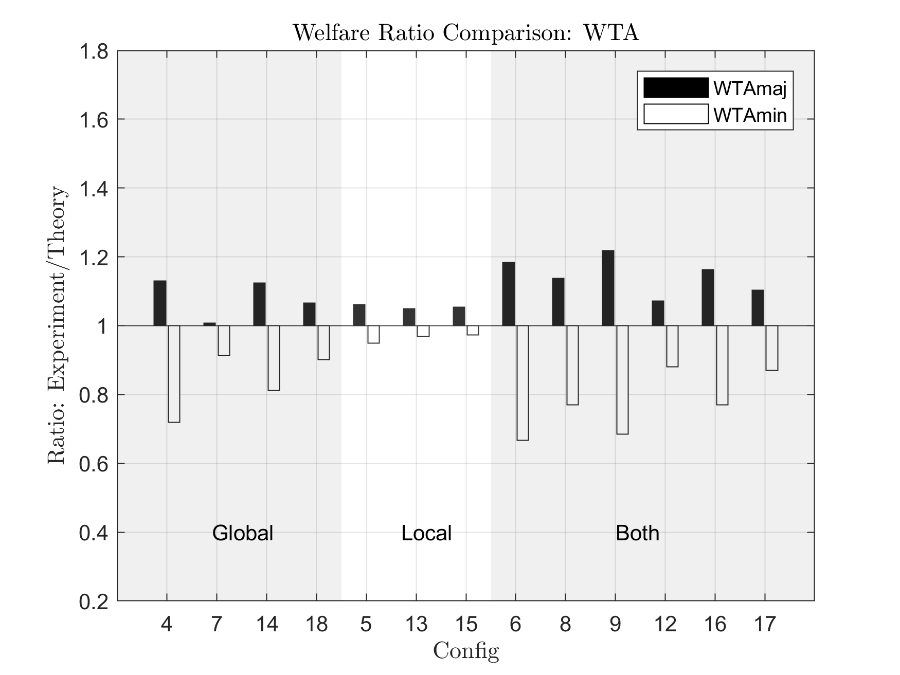
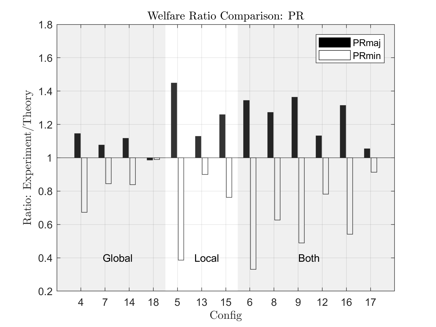
Figure 4: Ratio of welfare in the experiment to the theory.

Figure 3 shows the scatter plot of the theoretical and experimental welfare levels for each rule. The vertical (resp. horizontal) axis represents the experimental (theoretical) values. We see that the dots for the majority ($\bullet$) lie above the 45-degree line, while those for the minority ($\circ$) lie below it. This means that the behavioral bandwagon and Titanic effects caused an increase in the majority’s welfare and a decrease in the minority’s welfare. The trend is similarly observed under both rules, but its extent is more pronounced under PR. This pattern is clearly visible in Figure 4, which shows the ratio of the experimental welfare level divided by the theoretical welfare level for each configuration. Under both rules, the majority (resp. minority) bars extend above (below) the ratio value of 1. For both the majority and minority camps, the bars are longer under PR than WTA.

It is worth noting that the welfare predictions in the IC categories are remarkably close to those in the experiment, confirming the validity of the model in the IC environment and suggesting that the deviation of welfare from equilibrium arises due to behavioral effects related to being in the majority or minority.

Table 6: Average welfare comparison, theory vs. experiment.

Expected welfare of majority
	WTA				PR
	Theory	Experiment	Diff.(%)		Theory	Experiment	Diff.(%)
Global	0.552	0.598	+8.3%		0.563	0.610	+8.4%
Local	0.442	0.466	+5.4%		0.553	0.709	+28.1%
Both	0.560	0.641	+14.4%		0.571	0.712	+24.6%
Expected welfare of minority
	WTA				PR
	Theory	Experiment	Diff.(%)		Theory	Experiment	Diff.(%)
Global	0.409	0.343	$-16.1\%$		0.398	0.336	$-15.6\%$
Local	0.527	0.507	$-3.8\%$		0.367	0.252	$-31.4\%$
Both	0.403	0.310	$-23.0\%$		0.387	0.239	$-38.3\%$
Ex ante Gini coefficient
	WTA				PR
	Theory	Experiment	Diff.(%)		Theory	Experiment	Diff.(%)
Global	0.074	0.135	+81.7%		0.086	0.145	+69.0%
Local	0.040	0.034	$-15.2$%		0.031	0.060	+92.6%
Both	0.060	0.137	+128.2%		0.073	0.193	+163.6%

Table 6 shows the comparison of expected welfare between theory and experiment, averaged over configurations in each category. These numbers confirm that (i) welfare increases in the majority and decreases in the minority, and (ii) the differences are larger under PR than WTA in most cases. Table 6 also shows the ex ante Gini coefficients. We observe that inequality increases, except for the Local category under WTA.

4.3 Dependence on the local and global support rates

Figures 5 shows how the turnout rate (vertical axis) varies as a function of the local and global support rates for the preferred candidate (horizontal axis) in theory (+) and experiment ($\ast$). Here again, the Titanic effect and the behavioral bandwagon effect are visible. On the left-hand side of 0.5, the observed turnout is below the predicted turnout, and the inverse relationship holds on the right-hand side. These effects appear more clearly concerning the local support rate (the upper figures) than the global support rate (the bottom figures).

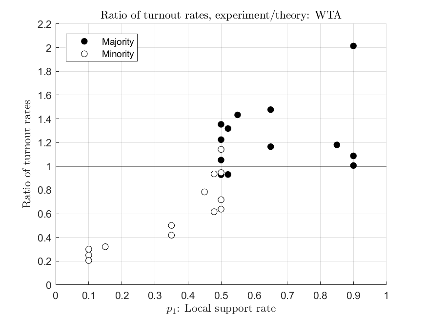
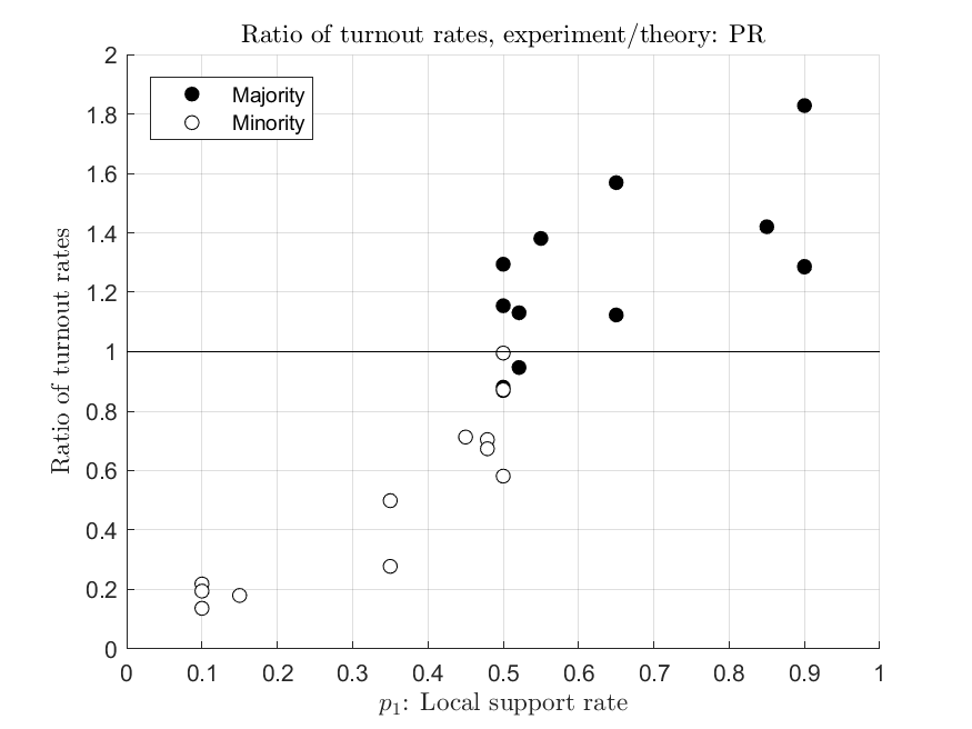
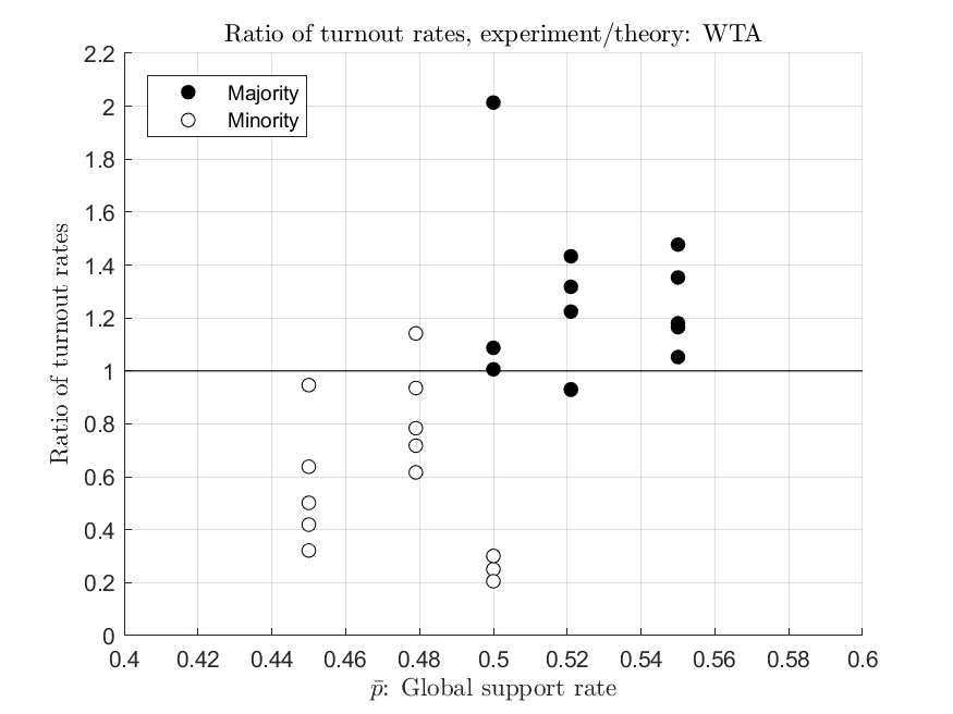
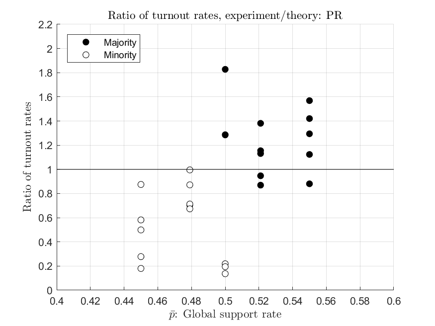
Figure 5: Ratio of the turnout rates as a function of the local support rate $p_{1}$ and the global support rate $\bar{p}$.

4.4 Regression analysis

We report regression results to further investigate turnout behavior at the individual level (Table 7). Two dependent variables are employed, concerning the voter turnout for each of WTA and PR. The first variable, [Experiment], is the normalized threshold chosen by each subject as the maximum cost acceptable for voting, divided by the range of voting costs (i.e., 200). Since the variable is bounded by the interval [0,1], a two-limit Tobit model is applied. The second dependent variable, [Experiment]$-$[Theory], measures the extent to which each subject’s turnout behavior deviates from the equilibrium. A generalized least squares model is employed for this regression. Random effect models are used for each regression, in order to account for the individual-specific effects of each subject who has made 18 decisions under each rule.

Table 7: Determinants of turnout, random effects regressions

[Experiment] [Experiment]$-$[Theory] Tobit GLS (1) WTA (2) PR (3) WTA (4) PR Local Majority $0.0315$ $0.0538^{*}$ $0.0081$ $0.0459^{**}$ $[0.0294]$ $[0.0277]$ $[0.0219]$ $[0.0210]$ Local Majority $\times$ Local Majority Share $-0.5503^{***}$ $-0.1867^{**}$ $0.1549^{**}$ $0.2381^{***}$ $[0.0915]$ $[0.0852]$ $[0.0679]$ $[0.0645]$ Local Minority $-0.0721^{**}$ $-0.1117^{***}$ $-0.0577^{**}$ $-0.0555^{**}$ $[0.0333]$ $[0.0315]$ $[0.0242]$ $[0.0235]$ Local Minority $\times$ Local Minority Share $0.9069^{***}$ $0.5897^{***}$ $0.6385^{***}$ $1.3009^{***}$ $[0.1441]$ $[0.1479]$ $[0.1021]$ $[0.1084]$ Global Majority $-0.0477$ $-0.0735^{**}$ $-0.0178$ $-0.0377$ $[0.0389]$ $[0.0364]$ $[0.0290]$ $[0.0276]$ Global Majority $\times$ Global Majority Share $2.7268^{***}$ $2.4255^{***}$ $1.5055^{**}$ $1.3617^{**}$ $[0.8014]$ $[0.7581]$ $[0.5960]$ $[0.5742]$ Global Minority $-0.0413$ $-0.0259$ $-0.0248$ $-0.0229$ $[0.0422]$ $[0.0398]$ $[0.0308]$ $[0.0299]$ Global Minority $\times$ Global Minority Share $1.7620^{*}$ $2.7850^{***}$ $1.7377^{**}$ $1.3906^{**}$ $[0.9726]$ $[0.9083]$ $[0.7075]$ $[0.6779]$ Local Population $-0.0034^{***}$ $-0.0003$ $0.0088^{***}$ $0.0114^{***}$ $[0.0013]$ $[0.0012]$ $[0.0009]$ $[0.0009]$ Local Population Share $0.2284^{***}$ $0.3747^{***}$ $0.1879^{***}$ $-0.2826^{***}$ $[0.0820]$ $[0.0769]$ $[0.0605]$ $[0.0579]$ Round $-0.0092^{***}$ $-0.0043^{***}$ $-0.0067^{***}$ $-0.0030^{***}$ $[0.0011]$ $[0.0010]$ $[0.0008]$ $[0.0008]$ Constant $0.5509^{***}$ $0.3966^{***}$ $-0.0246$ $0.0044$ $[0.1283]$ $[0.1251]$ $[0.0836]$ $[0.0840]$ Individual Traits Yes Yes Yes Yes Observations $3024$ $3024$ $3024$ $3024$ Overall model significance $470.37$ $443.86$ $818.72$ $1286.07$ Standard errors in brackets ^∗ $p<0.10$, ^∗∗ $p<0.05$, ^∗∗∗ $p<0.01$ Overall model significance is evaluated by Wald chi square statistic with the degree of freedom of 18.

Independent variables include those associated with subjects’ decision-making environments and individual characteristics. We also include the round number to capture the time trend of voting behavior. Since we have three groups in our elections (i.e., the human group and two computer groups), each factor of the voting configuration has both within and between-group aspects.

The majority dummy in the human group (i.e., Local Majority) takes the value 1 if each subject belongs to the majority in the human group and 0 otherwise. Note that the majority is defined in the ex-ante sense: it is the camp to which each subject is assigned with a higher probability than the other camp (i.e., $B$ if $p_{1}\neq 0.5$). The interaction term between the majority dummy and the share of the majority in the human group (i.e., Local Majority Share) expresses how large the majority occupies. The minority dummy (i.e., Local Minority) and its interaction term with its share in the human group (i.e., Local Minority Share) are defined similarly to those for the majority. Hence, the benchmark is when each subject is assigned to the two camps equally likely (i.e., $p_{1}=0.5$). We also define the counterparts in the whole electorate in the same way (i.e., Global Majority, Global Majority Share, Global Minority, and Global Minority Share).

The number of voters in the human group (i.e., Local Population) is a variable directly associated with the pivotality of each vote within the group. The larger the number of voters, the less likely each vote is to affect the outcome. The share of the human group in the whole electorate (i.e., Local Population Share) is related to the pivotality of the human group in the result. The larger the share of the human group, the more likely each vote affects the outcome.

We have seven control variables for each subject’s characteristics based on the post-experimental questionnaire. Specifically, we measured the extent to which the subjects feel obliged to vote, the extent to which they feel bothersome to vote, the subject’s perception of electoral effectiveness in general, and the degree of prosociality (putting the benefit of the whole ahead of the benefit of the individual). Subjects are also asked about their biological gender, whether or not they are science majors, and their experience of voting in national or local elections in the past (never or at least once).

Overall results

We mainly focus on the behavioral effects of majority/minority status and majority/minority share on the turnout deviation, i.e., [Experiment]$-$[Theory] in Columns (3) and (4) of Table 7. The signs of these effects and their relative magnitudes between WTA and PR are broadly consistent with our discussion of the Titanic and behavioral bandwagon effects based on the aggregated data in the previous subsections.

The effects of minority status and minority share

Local minority status negatively affects the turnout deviation. In Columns (3) and (4) of Table 7, this can be seen from the negative significant coefficient of Local Minority for both WTA and PR. On the other hand, the coefficient of Global Minority (i.e., being a majority in society) is negative, but not significant. The difference may be due to the fact that the subjects were not explicitly informed of their global minority/majority status, while their local minority/majority status was explicitly indicated on the screen.

The turnout deviation for minority voters decreases as the minority share decreases, at both local and global levels. This can be observed from the positive significant coefficients of the interaction terms Local Minority$\times$Local Minority Share and Global Minority$\times$Global Minority Share in Columns (3) and (4), suggesting that the degree of the Titanic effect increases as the degree of minority intensifies. Moreover, these variables also have positive significant coefficients in Columns (1) and (2), implying that as the minority share decreases, minority turnout itself decreases, and this decrease is sharper than theory.

The effects of majority status and majority share

Similar observations can be made for the behavior of majority voters. Local majority status positively affects the turnout deviation at least under PR. In Columns (3) and (4) of the table, this can be observed from the positive significant coefficient of Local Majority for PR. The coefficient is positive, but not significant for WTA. The coefficient of Global Majority is not significant, for which the same explanation as for Global Minority may apply.

The turnout deviation for majority voters increases as the majority share increases, as can be observed from the positive significant coefficients of Local Majority$\times$Local Majority Share and Global Majority$\times$Global Majority Share. The degree of the behavioral bandwagon effect increases as the degree of majority intensifies. Moreover, Local Majority$\times$Local Majority Share is negative significant in Columns (1) and (2), implying that as the local majority share increases, majority turnout itself decreases, and this decrease is less intensive than theory. On the other hand, Global Majority$\times$Global Majority Share is positive significant in Columns (1) and (2), that is, majority turnout itself increases as the global majority share increases.

Comparison of rules

How do these effects vary across the rules? The effect of local minority status (i.e., Local Minority) does not significantly differ between WTA and PR. However, as the local minority share decreases, the turnout deviation for minority voters decreases more substantially under PR than under WTA. Indeed, in Columns (3) and (4) of the table, the coefficient of Local Minority$\times$Local Minority Share under PR is more than twice that under WTA. This is consistent with what we observed from the aggregated data in Section 4.1: in Panel B of Table 5(b), the deviation of minority turnout from the theoretical prediction is larger in absolute value for PR than WTA, for most voting configurations in categories Local and Both.

The effect of local majority status (i.e., Local Majority) is significant for PR, but not for WTA. Moreover, as the local majority share increases, the turnout deviation for majority voters increases more sharply under PR than under WTA, which can be seen by comparing the coefficients of Local Majority$\times$Local Majority Share between PR and WTA. This is somewhat consistent with Panel A of Table 5(b), in which the deviation of majority turnout from theory is larger for PR than WTA, at least for the voting configurations in category Local.

Finally, the corresponding effects for global minority/majority voters do not significantly differ between the two rules. This can be checked by comparing the coefficients of Global Minority/Majority and their interaction terms with the minority/majority share between WTA and PR.

Other findings

The coefficients of Local Population on turnout, Columns (1) and (2), are negative significant (only for WTA), whereas the coefficients on the turnout deviation, Columns (3) and (4), are positive significant for both rules. This is consistent with the general wisdom that turnout decreases as the pivotal probability decreases in large election, but turnout in the experiment did not decrease as much as theory suggests.

The coefficients of Local Population Share on turnout, Columns (1) and (2), are positive significant for both rules. This is also consistent with the theory that turnout in a group increases as the group becomes more pivotal in society. The coefficient on the turnout deviation, Columns (3) and (4), is positive significant for WTA, and negative and significant for PR, suggesting that turnout increases more than theory under WTA, and less than theory under PR.

The variables on subjects’ individual characteristics are not significant, suggesting that individual characteristics did not affect turnout behavior of the subjects in our experiment.

5 Conclusion

We conducted an online experiment in a controlled environment to examine the turnout and welfare achieved under two groupwise vote aggregation rules. Votes are first aggregated to determine the weight allocation between candidates in each group, which is then summed to determine the winner. We observed the Titanic effect and the behavioral bandwagon effect, i.e., subjects from a minority camp were less likely to vote than theoretically predicted, while those from a majority camp were more likely. Such effects were observed more acutely under the proportional rule than under the winner-take-all rule.

One of the specific features of our experiment, which differs from existing ones in the literature, is that there are multiple groups within the whole electorate. Consequently, we can distinguish the effects of being in the local majority or minority from those of being in the global majority or minority on voters’ decisions to turn out. From our regression results, we observe that the turnout rate correlates more strongly with being local majority or minority than with being global majority or minority.

The consequences of these effects on democratic decision making are twofold. The first concerns efficiency of the electoral outcome. We observe that the winning probability of the majority candidate is higher in the experiment than in equilibrium, due to the high (resp. low) turnout of the majority (resp. minority) supporters. The second concerns the distribution of welfare among voters. Expected welfare increased (resp. decreased) in the majority (resp. minority) camp, suggesting that the above-mentioned behavioral effects may lead to an undesirable outcome in terms of equality, in exchange for the gain in efficiency.

In our experiment, we assigned human subjects to one of the three groups, with the other two groups consisting of automated voters adopting the equilibrium strategy. This method lightened cognitive burden on the subjects, making it easier for them to understand the overall election structure. It also enabled us to eliminate data dependence across groups and make our statistical analyses tractable. However, given that the automated voters’ equilibrium play may differ depending on the aggregation rules, direct comparison of the rules through our experimental results obtained by the composition of the human subjects and automated voters has become less obvious. We leave the fully comprehensive analysis comparing our results with those obtained when all groups are made up of human subjects for future research.

References

- Agranov et al. (2018) Agranov, Marina, Jacob K Goeree, Julian Romero, and Leeat Yariv. 2018. “What makes voters turn out: The effects of polls and beliefs.” Journal of the European Economic Association 16 (3):825–856.
- Aguiar-Conraria, Magalhães, and Vanberg (2016) Aguiar-Conraria, Luís, Pedro C Magalhães, and Christoph A Vanberg. 2016. “Experimental evidence that quorum rules discourage turnout and promote election boycotts.” Experimental Economics 19 (4):886–909.
- Barberà and Jackson (2006) Barberà, S. and M. O. Jackson. 2006. “On the weights of nations: Assigning voting weights in a heterogeneous union.” Journal of Political Economy 114:317–339.
- Barnfield (2020) Barnfield, Matthew. 2020. “Think Twice before Jumping on the Bandwagon: Clarifying Concepts in Research on the Bandwagon Effect.” Political Studies Review 18 (4):553–574.
- Duch, Grossmann, and Lauer (2020) Duch, Matthias L, Max RP Grossmann, and Thomas Lauer. 2020. “z-Tree unleashed: A novel client-integrating architecture for conducting z-Tree experiments over the Internet.” Journal of Behavioral and Experimental Finance 28:100400.
- Faravelli, Kalayci, and Pimienta (2020) Faravelli, Marco, Kenan Kalayci, and Carlos Pimienta. 2020. “Costly voting: A large-scale real effort experiment.” Experimental Economics 23 (2):468–492.
- Greiner (2015) Greiner, Ben. 2015. “Subject pool recruitment procedures: organizing experiments with ORSEE.” Journal of the Economic Science Association 1 (1):114–125.
- Grillo (2017) Grillo, Alberto. 2017. “Risk aversion and bandwagon effect in the pivotal voter model.” Public Choice 172 (3):465–482.
- Großer (2020) Großer, Jens. 2020. “Voting game experiments with incomplete information: a survey.” In Handbook of Experimental Game Theory. Edward Elgar Publishing.
- Großer and Schram (2010) Großer, Jens and Arthur Schram. 2010. “Public opinion polls, voter turnout, and welfare: An experimental study.” American Journal of Political Science 54 (3):700–717.
- Herrera, Morelli, and Palfrey (2014) Herrera, Helios, Massimo Morelli, and Thomas Palfrey. 2014. “Turnout and power sharing.” The Economic Journal 124 (574):F131–F162.
- Hoffmann and Renes (2021) Hoffmann, Timo and Sander Renes. 2021. “Flip a coin or vote? An experiment on the implementation and efficiency of social choice mechanisms.” Experimental Economics :1–32.
- Irwin and Van Holsteyn (2000) Irwin, Galen and Joop JM Van Holsteyn. 2000. “Bandwagons, underdogs, the Titanic, and the Red Cross: the influence of public opinion polls on voters.” In Communication presented at the 18th Congress of the International Political Science Association, Québec. 1–5.
- Kartal (2015) Kartal, Melis. 2015. “Laboratory elections with endogenous turnout: proportional representation versus majoritarian rule.” Experimental Economics 18 (3):366–384.
- Kikuchi and Koriyama (2023) Kikuchi, Kazuya and Yukio Koriyama. 2023. “The winner-take-all dilemma.” Theoretical Economics 18 (3):917–940.
- Koriyama et al. (2013) Koriyama, Yukio, Jean-François Laslier, Antonin Macé, and Raphael Treibich. 2013. “Optimal Apportionment.” Journal of Political Economy 121:584–608.
- Koriyama and Wang (2024) Koriyama, Yukio and Zijun Wang. 2024. “Does the winner-take-all rule protect minority?” mimeo .
- Kurz, Maaser, and Napel (2017) Kurz, S., N. Maaser, and S. Napel. 2017. “On the Democratic Weights of Nations.” Journal of Political Economy 125:1599–1634.
- Levine and Palfrey (2007) Levine, David K and Thomas R Palfrey. 2007. “The paradox of voter participation? A laboratory study.” American Political Science Review 101 (1):143–158.
- Morton and Ou (2015) Morton, Rebecca and Kai Ou. 2015. “What motivates bandwagon voting behavior: Altruism or a desire to win?” European Journal of Political Economy 40 (PB):224–241.
- Palfrey and Rosenthal (1983) Palfrey, Thomas and Howard Rosenthal. 1983. “A strategic calculus of voting.” Public Choice 41 (1):7–53.
- Palfrey and Rosenthal (1985) Palfrey, Thomas R and Howard Rosenthal. 1985. “Voter participation and strategic uncertainty.” American Political Science Review 79 (1):62–78.
- Schram and Sonnemans (1996) Schram, Arthur and Joep Sonnemans. 1996. “Voter turnout as a participation game: An experimental investigation.” International Journal of Game Theory 25 (3):385–406.