Decoupled Anisotropic Buchdahl’s Relativistic Models in Theory
Abstract
This paper constructs three different anisotropic extensions of the existing isotropic solution to the modified field equations through the gravitational decoupling in theory. For this, we take a static sphere that is initially filled with the isotropic fluid and then add a new gravitational source producing anisotropy in the system. The field equations now correspond to the total matter configuration. We transform the radial metric component to split these equations into two sets characterizing their parent sources. The unknowns comprising in the first set are determined by considering the Buchdahl isotropic solution. On the other hand, we employ different constraints related to the additional gravitational source and make the second system solvable. Further, the constant triplet in Buchdahl solution is calculated by means of matching criteria between the interior and exterior geometries at the spherical boundary. The mass and radius of a compact star LMC X-4 are used to analyze the physical relevancy of the developed models. We conclude that our resulting models II and III are in well-agreement with acceptability conditions for the considered values of the parameters.
Keywords: Modified theory;
Anisotropy; Gravitational decoupling.
PACS: 04.40.Dg; 04.50.Kd; 04.40.-b.
1 Introduction
Cosmologists have recently made significant discoveries that challenge the perception of the arrangement of astrophysical structures in our universe. Rather than a random distribution, these structures appear to be systematically organized, sparking considerable interest among researchers. The detailed study of such interstellar bodies has become a focal point for scientists seeking to figure out the mystery of the accelerated expansion of the cosmos. It has become evident through various experiments that our universe contains abundance of a force countering the pull of gravity, and thus driving such expansion. This mysterious force is referred to the dark energy due to its obscure nature that continues to confuse researchers. While general relativity () explains this expansion up to some extent, it grapples with issues related to the cosmological constant. Therefore, some extensions of this theory need to be proposed.
A straightforward generalization to is the theory that represents a significant advancement in the field of theoretical physics. It introduces a modification to the Einstein-Hilbert action, where the roles of the Ricci scalar and its generic function are interchanged. This theory has provided promising results and has been employed to investigate self-gravitating systems [1]-[5]. Astashenok et al. [6] investigated the causal limit of maximum mass for stars in this modified framework. Their findings led to the conclusion that the secondary component of the compact binary GW190814 is likely to be a neutron star, a black hole, or possibly a rapidly rotating neutron star, ruling out the possibility of it being a strange star. There is a body of literature, pointing out such important works by various researchers [7]-[12]. Bertolami et al. [13] initially presented the idea of studying the fluid-geometry interaction in framework and executed this by combining the matter Lagrangian density and as a single function. This notion prompted astronomers to put their focus on the discussion of the rapid expansion of the universe [14].
Soon after this, Harko et al. [15] generalized this concept at the action level, and pioneered a new gravitational theory. This was named as theory where the effects of geometry and matter configuration are coupled through and trace of the energy-momentum tensor () . This generalized function results in the non-conserved system, hence, an extra force (that depends on physical parameters like pressure and density [16]) appears in the gravitational field which forces the test particles to move in a non-geodesic path. Houndjo [17] employed a minimal model of this modified theory to explain the conversion of the matter-dominated phase into late-time acceleration era successfully. Among several models, gained much importance in the literature that produces physically acceptable compact interiors. This model is adopted by Das et al. [18] to establish a gravastar-like model consisting of three layers, each of them is represented by different equations of state. Multiple stellar interiors have been discussed by using various approaches in the context of this modified model [19]-[25]. One significant notion of theory is that it considers the quantum effect, leading the possibilities of particle production. This aspect holds much importance in astrophysical research as it posits a connection between quantum theory and gravity. Some notewrothy applications of this theory in both astrophysics and cosmology can be seen in [26]-[28]. Recently, Zaregonbadi et al. [29] have examined the viability of this modified theory to explore the effects of dark matter on the galactic scale.
The standard model of the cosmos is believed to be mainly based on the homogeneity and isotropy at a large-scale, however, there exists pressure anisotropy at some small-scales [30]-[32]. Further, the geometry of compact objects guarantees the presence of anisotropic pressure and inhomogeneous fluid distribution. The former factor appears when there is a difference between the pressure in both radial and transverse directions. There is a class of components that produces anisotropy in the interior configuration such as phase transitions [33], pion condensation [34], neutron stars surrounded by a strong electromagnetic field [35], and some other factors [36, 37]. Another factor that causes the anisotropy is the gravitational effects produced by the tidal forces [38]. The isotropy of our universe has recently been examined by analyzing X-rays coming from galactic clusters [39]. The same strategy has then been carried out on massive structures, and it was concluded that the nature of cosmos is anisotropic [40]. The pressure anisotropy is thus much significant to be studied and affects several physical characteristics like the energy density, gravitational redshift and mass, etc., of a self-gravitating system.
The self-gravitating celestial objects represented by non-linear gravitational field equations in or other modified theories prompted astrophysicists to obtain their exact/numerical solutions. The compact interiors could be of physical interest only if the corresponding formulated solution fulfills the required conditions. Multiple techniques, in this regard, have recently been suggested, one of them is the gravitational decoupling that is employed to model a compact interior possessing multiple sources including anisotropy, heat dissipation, shear, etc. The initial idea of this technique was based on the fact that the field equations comprising different sources can be decoupled into multiple sets, and thus it becomes an easy task to solve each set individually. Ovalle [41] recently pioneered the minimal geometric deformation (MGD) scheme which provides some enticing ingredients to formulate physically acceptable stellar solutions in the braneworld. Following this, an isotropic spherically symmetric matter distribution was discussed by Ovalle and Linares [42] who formulated an analytical solution in the braneworld and found it consistent with Tolman-IV ansatz. Casadio et al. [43] obtained the Schwarzschild geometry in the context of Randall-Sundrum braneworld theory by extending the above strategy.
Ovalle and his collaborators [44] adopted a spherically symmetric isotropic interior and developed its physically feasible anisotropic version using the MGD scheme. Sharif and Sadiq [45] introduced the straightforward extension of this technique to the charged case where they constructed two different anisotropic counterparts of Krori-Barua metric potentials and discussed their stability. Multiple metric ansatz have been extended to obtain their corresponding anisotropic analogs through MGD in modified theory [46]. The Durgapal-Fuloria metric coefficients have been taken as a seed isotropic source through which several physically relevant anisotropic solutions were obtained [47]. Different researchers proposed the anisotropic extensions of isotropic Heintzmann as well as Tolman VII solutions and found them stable in the considered range [48, 49]. Sharif and Ama-Tul-Mughani [50] took the axial spacetime into account and formulated their corresponding well-behaved solutions. We have also obtained such charged/uncharged anisotropic analogs of Krori-Barua ansatz in a strong non-minimally coupled gravitational theory [51]-[54].
This article formulates three different anisotropic solutions that are, in fact, the extensions of an isotropic interior to the additional matter source coupled gravitationally to the seed source in framework. The following lines present how this paper is organized. The fundamentals of the modified theory and its relevant field equations corresponding to the total (seed and newly added) matter source are formulated in the next section. Section 3 introduces the MGD transformation that helps to decouple the field equations into two sets. We then adopt the Buchdahl’s solution in section 4 and calculate the unknown constants through boundary conditions. Section 5 presents some conditions whose fulfillment leads to physically acceptable model. Three newly developed anisotropic solutions and their graphical interpretation are provided in section 6. Lastly, we summarize our outcomes in the last section.
2 Gravity
The Einstein-Hilbert action for the modified theory becomes (with ) after the inclusion of an additional field as [15]
| (1) |
where is the fluid’s Lagrangian density. We suppose an extra source to be gravitationally coupled with the parent matter configuration whose corresponding Lagrangian is denoted by . The decoupling parameter explains how much an extra source influences the physical properties characterizing a self-gravitating system. Also, the metric tensor in this case provides the determinant indicated by . The least action principle is applied on the action (1), leading to the field equations given by
| (2) |
where and describe the geometric sector and the interior fluid distribution, respectively. The later term is further classified as
| (3) |
Here is the additional fluid source. Moreover, the effective matter sector is divided into the usual and modified . The later term takes the form
| (4) | |||||
where and mean and , respectively. Furthermore, is the D’Alembert operator and is the covariant divergence. Also, we adopt ( is an isotropic pressure), leading to .
We consider that the geometrical structure is initially filled with an isotropic fluid which can be expressed through the following
| (5) |
where and are the energy density and four-velocity, respectively. We obtain the trace of Eq.(2) as follows
Since the action of this theory involves matter-geometry coupled functional, the disappearance of the matter term, i.e., (or vacuum case) reduces all our results in gravity. Moreover, the non-zero divergence of the usual is observed in this theory due to such strong interaction. Resultantly, an additional force appears in the field of self-gravitating object that alters the geodesic path of the moving test particles. Its mathematical expression is given by
| (6) |
where .
We consider a spherical interior geometry that is distinguished from the exterior region at the hypersurface given by the following line element
| (7) |
where and . The corresponding four-velocity now takes the form in terms of temporal metric component as
| (8) |
In order to have some meaningful results, we adopt a standard modified model. Although the literature presents several matter-geometry coupled (minimal as well as non-minimal) models, however, we adopt a minimal one which is given by
| (9) |
where and is a real-valued constant. There are two main reasons behind this choice highlighted as
-
•
For complicated functionals containing exponential, logarithmic, or polynomials terms of , or higher-order curvature terms such as , we will obtain a very complicated form of the field equations. So, the problem appears when it comes to split those equations into two sets using MGD technique (following section elaborates MGD methodology thoroughly). In such cases, we may be unable to obtain two new sectors characterizing their parent fluid sources.
-
•
On the other hand, in the case of complex functionals, an issue appears when we deal with matching conditions across the spherical interface. Therefore, in order to adjust these issues, we choose the functional given in Eq.(9).
Moreover, Ashmita et al. [55] derived potential slow-roll parameters by adopting multiple inflation potentials in this gravitational theory and found their results to be consistent with the experimental data only when . This model has also been used to formulate physically relevant anisotropic version of the interior Tolman-Kuchowicz spacetime [56]. We have developed acceptable decoupled solutions corresponding to anisotropic configuration in this theory [57, 58].
The spherical spacetime (7) produces the field equations corresponding to the modified model (9) as
| (10) | ||||
| (11) | ||||
| (12) |
where the entities along with appear as the corrections and prime means . Moreover, we obtain the generalized form of Tolman-Opphenheimer-Volkoff equation from (6) corresponding to the model (9) as
| (13) |
which verifies the nature of this extended theory of gravity to be non-conserved. Since Eq.(13) is a combination of different forces that maintain the hydrostatic equilibrium inside a celestial object, it plays an important role to study the interior’s structural changes. It is observed that the extraction of the solution of a system (10)-(12) becomes obscure due to the entanglement of a large number of unknowns, i.e., . Therefore, it becomes necessary to adopt some constraints, otherwise, the system cannot be solved uniquely. In this context, a systematic scheme [44] is adopted to fulfill our requirement.
3 Minimal Gravitational Decoupling
Gravitational decoupling is an efficient approach that transforms the metric potentials in a new reference frame and makes it easy to construct the solution of highly non-linear field equations representing compact systems. For this, a new line element is considered as a solution to the field equations (10)-(12) given by
| (14) |
Following equations transform the metric potentials and decouple the field equations as
| (15) |
where and correspond to and components, respectively. Gravitational decoupling offers two different techniques, i.e., minimal and extended deformations. The main difference between minimal and extended decoupling schemes is that the geometric deformation is applied only on the radial metric component in the former case, leaving temporal coefficient as an invariant quantity [59]. However, in the later scenario, both temporal as well as radial potentials are deformed to covert the field equations in a new reference frame [60]. Moreover, the MGD technique works as long as the interaction between the matter sources is purely gravitational, implying that each fluid source must be conserved individually. This is in contrast with the extended decoupling approach in which the total fluid configuration is conserved but the non-conservation phenomenon occurs when it comes to individual systems of equations. The transfer of the energy between different source is also allowed in this scenario. Further, the deformation function plays a crucial role in the process of gravitational decoupling. Its selection is based on the specific characteristics of the problem and the intended simplification, with the additional requirement of ensuring the spherical symmetry of the solution. In the current setup, we have . Hence, Eq.(15) switches into
| (16) |
where . It must be kept in mind that such a linear mapping does not bother the considered spherical symmetric. We apply the transformation (16) on the system (10)-(12) to divide into two different sets corresponding to and . The first set corresponds to the initial (isotropic) source and is given by
| (17) | ||||
| (18) | ||||
| (19) |
The simultaneous solution of Eqs.(17) and (18) results in the state variables as
| (20) | ||||
| (21) |
Contrariwise, the field equations representing the additional matter distribution () are obtained as
| (22) | ||||
| (23) | ||||
| (24) |
It is interesting to note that both (seed and new) sources are individually conserved, and hence, the energy’s exchange between them is not allowed in this scheme. Further, we successfully decouple the set of equations (10)-(12) that makes easier to solve both sets independently. There appear four unknowns () in Eqs.(20) and (21), thus we must require a well-behaved metric ansatz to equal the number of unknowns to that of equations. Also, four unknowns () are appeared in the system (22)-(24), a unique solution shall be obtained by adopting a constraint on -sector. Since the additional source makes the initial matter source anisotropic, we identify the matter determinants as follows
| (25) |
which help to define the total anisotropic factor as
| (26) |
verifying its disappearance for the case when , i.e., the effect of a new matter source is removed.
4 Buchdahl Solution and Boundary Conditions
This section is devoted to the formulation of a solution corresponding to the first set given by (20) and (21). We have already discussed that a particular form of metric potentials is required to solve the system. In this context, Buchdahal ansatz [61] has attracted significant attention among researchers. This assumption has proven valuable in investigating almost all physically viable known super-dense star models. Vaidya and Tikekar [62] further refined the Buchdahl ansatz and discussed spheroidal geometries for the 4-dimensional hypersurface. Such a particular spheroidal condition has been proved to be highly effective in obtaining exact solutions to the field equations, a task that proves challenging in numerous other scenarios. Kumar et al. [63] extensively explored this particular spacetime, focusing on charged compact objects coupled with the isotropic fluid distribution. Additionally, Sharma et al. [64] determined the maximum attainable masses and radii for various values of the surface density within the Vaidya-Tikekar spacetime. Maurya et al. [65] adopted this metric and discussed eight different cases for Buchdahl’s dimensionless parameter and found all of them valid at every point within the interior geometry. Various authors used this metric to produce viable as well stable charged/uncharged interiors in the contexts of and theory [66]-[68]. This metric is adopted as follows
| (27) | |||||
| (28) | |||||
| (29) | |||||
| (30) | |||||
where and are unknown quantities that must be determined to perform the graphical analysis.
In this perspective, the junction (or matching) conditions play a vital role in the study of structural characteristics of a compact object at some boundary surface (). The interior geometry now becomes in terms of ansatz (27) and (28) as
| (31) |
whose corresponding exterior spacetime is described by the Schwarzschild metric. This is given as follows
| (32) |
where shows the total mass. The first fundamental form of these constraints provide continuity of the metric potentials at the hypersurface as
providing the following expressions by employing the metrics (31) and (32) as
| (33) | |||||
| (34) |
| 0 | 0.25 | 0.5 | 0.75 | 1 | 1.25 | |
|---|---|---|---|---|---|---|
| 3.6039 | 3.4065 | 3.2253 | 3.0585 | 2.9047 | 2.7626 | |
| 3.6616 | 3.8256 | 3.9892 | 4.1524 | 4.3153 | 4.4777 | |
| 4.5616 | 4.5616 | 4.5616 | 4.5616 | 4.5616 | 4.5616 |
Since we have two equations and three unknowns, we need one more constraint. For this, we use the second fundamental form that claims that the isotropic pressure disappears at the boundary, i.e., . Thus, Eq.(30) provides
| (35) |
By solving Eqs.(33)-(35) simultaneously, we get the triplet as
| (36) | |||||
| (37) | |||||
| (38) |
where is provided by
| (39) | ||||
| (40) |
We use the calculated values of the mass and radius as and , respectively, of a compact star candidate LMC X-4 [69] to evaluate the above constant triplet. Table 1 provides these values corresponding to different choices of the model parameter. It is observed that the constant () is in inverse (direct) relation with the parameter , however, the unknown is not dependent on .
5 Physical Acceptability Conditions of a Compact Model
There are several criteria in the literature to check physical acceptability of compact structures [70]-[74]. Some other works are [75]-[78]. They are highlighted as follows.
-
•
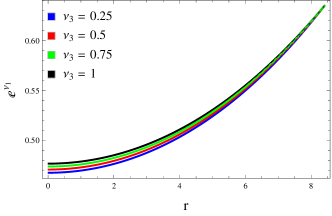
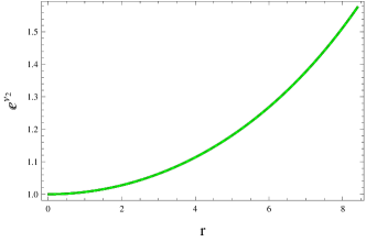
One of the fundamental aspects is the existence of geometric singularities inside the star. The behavior of the metric components should be positively increasing and free from singularity in an acceptable self-gravitating interior. The metric coefficients (27) and (28) in the core of star become
and their first derivatives are
where . We notice that the above both derivatives disappear at the center implying the regularity of these potentials. Figure 1 reveals that they are minimum at and increasing outwards to reach their maximum at the spherical surface.
-
•
The profile of matter determinants such as energy density and pressure components should be finite and positive everywhere. Further, they must reach their maximum (minimum) at (). Likewise, the decreasing trend of these variables towards the boundary can also be assured if their first derivative disappears at and negative outwards.
-
•
The mass of the spherical stellar structure is defined by
(41) The mass-radius ratio, known as the compactness, measures that how tightly the particles are bound with each other in a self-gravitating system. Mathematically, we have
(42) Its value must be less than everywhere in a spherical interior [61]. We can also describe the surface redshift in terms of mass or compactness of a star. This is given as
(43) Since we are discussing anisotropic matter distribution, the redshift reaches its maximum by at the boundary surface to get a feasible model [79].
-
•
Another key feature to check feasibility of the stellar model is the energy conditions which are in fact linear combinations of the matter determinants. These are given as follows
(44) Among these conditions, the dominant energy bounds (i.e., and ) are the most important because they demand and everywhere.
-
•
Different techniques have been suggested in the literature to check the stability of the compact stars, one of them is based on the sound speed whose radial and tangential components are and , respectively. Abreu et al. [80] suggested that if the speed of light is greater than that of sound (i.e., ), the causality would be preserved in a system. Likewise, Herrera [81] proposed that if the total radial force changes its sign throughout the evolution, then the idea of cracking would occur in the interior fluid. It must be avoided to obtain a stable model. He provided that the cracking cannot be occurred only if holds.
6 Formation of Different Anisotropic Models
Here we consider two sources characterizing different matter distributions, the unknowns are increased in the field equations. Therefore, we choose three different constraints to make such differential equations solvable. They are given by
-
•
Model I: Density-like constraint
-
•
Model II: Pressure-like constraint
-
•
Model III: A linear equation of state
6.1 Model I
We consider a constraint depending on the energy density of the original and anisotropic source to obtain solution to the total interior fluid. This is given as follows [82]
| (45) |
We use Eqs.(20) and (23) in (45), and obtain the differential equation as
| (46) |
In terms of Buchdahl’s ansatz (27) and (28), the above equation takes the form
| (47) |
The above equation contains one unknown (i.e., the deformation function ). However, the exact solution of this equation is not possible because of the terms appearing in the square root. Therefore, we use the numerical integration to make this function known. For this purpose, we use the initial condition by providing the range of the radius of the considered star. The corresponding deformed component can be calculated by
| (48) |
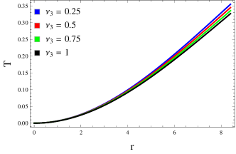
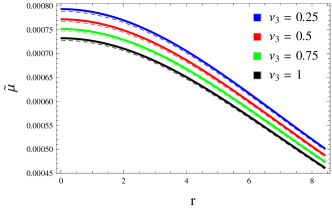
We perform the graphical analysis of the obtained deformation function and its corresponding matter determinants, anisotropy, energy conditions and some other parameters for the considered modified model (9). Moreover, we choose and to study the effect of decoupling strategy and the modified gravity on the interior of a compact star. The deformation function obtained from Eq.(47) does not depend on the decoupling parameter, thus its variation with respect to different values of the model parameter is plotted in Figure 2. It is observed that this function possesses increasing trend outwards, however, it takes smaller values for increasing .
The corresponding matter variables such as effective energy density, effective radial/tangential pressures and anisotropy are calculated through Eqs.(25) and (26). The trend of these variables is plotted in Figure 3, indicating an acceptable behavior. We notice that the energy density (pressure components) decreases (increase) with the increment in . However, they decrease by increasing the model parameter. Such a behavior can be observed by the numerical values provided in Tables 2 and 3. Further, the zero radial pressure at the spherical boundary is observed for each parametric value (upper right plot). The anisotropic factor, in this case, becomes null in the core and increases, otherwise. The parameters in Figure 4 possess increasing and acceptable profile throughout. The energy density in Eq.(41) corresponds to the total matter source involving modified corrections, thus the mass function is dependent on the decoupling and model parameters. The smaller values of both parameters and provide more massive interiors (upper left plot). Figure 5 shows the dominant energy bounds, displaying positive profile and thus leading to a viable solution. Figure 6 (lower plot) declares that our resulting model I is physically unstable because there occurs a cracking in the interior for every parametric choice.
| 0 | 0.25 | 0.5 | 0.75 | |
|---|---|---|---|---|
| 1.06251015 | 1.03161015 | 1.00581015 | 9.79971014 | |
| 6.67851014 | 6.55011014 | 6.36951014 | 6.16211014 | |
| 1.27581035 | 1.23731035 | 1.19381035 | 1.15611035 | |
| 0.178 | 0.174 | 0.168 | 0.163 | |
| 0.245 | 0.237 | 0.231 | 0.221 |
| 0 | 0.25 | 0.5 | 0.75 | |
|---|---|---|---|---|
| 1.05481015 | 1.02641015 | 9.98161014 | 9.72211014 | |
| 6.62631014 | 6.49791014 | 6.34271014 | 6.13671014 | |
| 1.28781035 | 1.24811035 | 1.20011035 | 1.16891035 | |
| 0.142 | 0.137 | 0.133 | 0.129 | |
| 0.179 | 0.174 | 0.168 | 0.164 |
6.2 Model II
In this subsection, we construct our second model by choosing the following constraint [83]
| (49) |
Using Eqs.(21) and (24) in the above equation, we have
| (50) |
that, in terms of the ansatz (27) and (28), leading to
| (51) |
The above equation provides the deformation function as
| (52) |
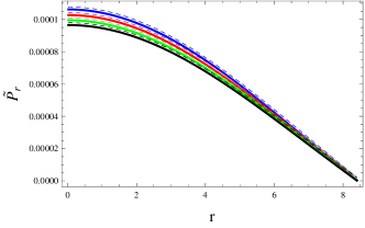
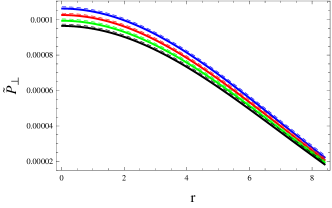
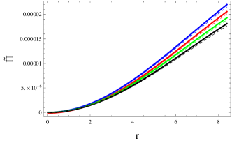
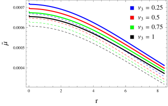
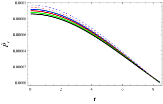
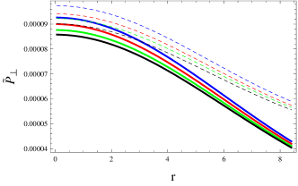
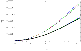
Figure 7 exhibits the plot of the above radial deformation function for the considered pressure-like constraint with respect to the chosen values of parameters. We observe that this function initially increases for all values of model parameter, i.e., , and then decreases to reach its minimum at the hypersurface. The effective matter determinants along with anisotropic factor corresponding to the above deformation function can be obtained by making use of Eqs.(25) and (26). We also examine the profile of such effective quantities in Figure 8. We find from the upper left plot that the energy density possesses the same (opposite) behavior as that of the first model near the center (spherical boundary). Tables 4 and 5 provide the numerical values that confirm such profile of these matter determinants. Further, both pressure ingredients and anisotropy show a consistent behavior. The radial pressure and anisotropic factor are found to be null at the boundary and center, respectively (right plots).
| 0 | 0.25 | 0.5 | 0.75 | |
|---|---|---|---|---|
| 1.01931015 | 9.91871014 | 9.66591014 | 9.43711014 | |
| 6.82831014 | 6.64511014 | 6.43911014 | 6.30261014 | |
| 1.39241035 | 1.35271035 | 1.31421035 | 1.26491035 | |
| 0.179 | 0.175 | 0.169 | 0.162 | |
| 0.245 | 0.235 | 0.229 | 0.219 |
| 0 | 0.25 | 0.5 | 0.75 | |
|---|---|---|---|---|
| 9.34621014 | 9.09461014 | 8.86591014 | 8.65981014 | |
| 7.10261014 | 6.91931014 | 6.71331014 | 6.55411014 | |
| 1.65451035 | 1.59561035 | 1.55711035 | 1.49821035 | |
| 0.169 | 0.168 | 0.163 | 0.161 | |
| 0.238 | 0.227 | 0.218 | 0.215 |
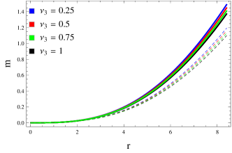
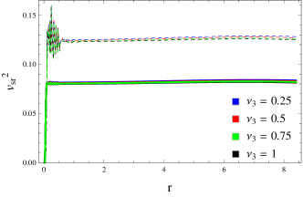
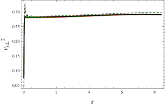
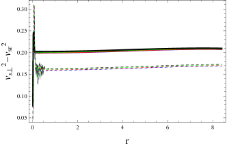
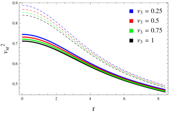
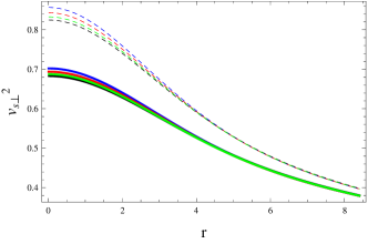
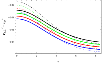
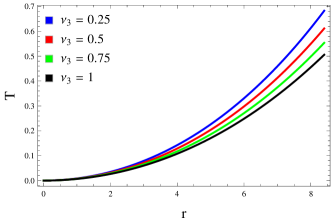
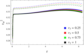
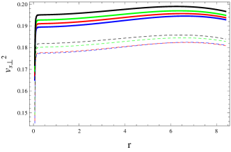
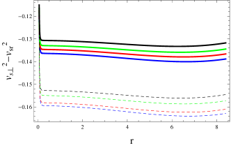
Figure 9 displays the variation in multiple factors with respect to and parametric values, and we find them consistent with observed data. Since we observe the matter triplet to be positive everywhere, the dominant energy bounds are only needed to check. We plot them in Figure 10 and deduce that the corresponding solution is viable. We also check the stability of the resulting solution in Figure 11, showing that our model II becomes stable through both criteria (sound speed and cracking approach).

6.3 Model III
Here, we assume a linear equation that connects different components of -sector given as follows [84]
| (53) |
where and are real-valued constants whose different values can be taken to check how the corresponding solution is influenced by these unknowns. Making use of Eqs.(23) and (24) in the above linear equation yields
| (54) |
One can involve component in Eq.(53), however, its presence will make the above equation more complicated due to the appearance of second order derivatives of the metric potentials. Joining the metric ansatz (27) and (28) with (54), we get
| (55) |
This is first order differential equation in whose analytical solution is not possible due to the appearance of a term in the square root. Therefore, we employ a numerical integration with an initial condition to obtain the deformation function for and .
| 0 | 0.25 | 0.5 | 0.75 | |
|---|---|---|---|---|
| 9.55351014 | 9.27791014 | 9.00511014 | 8.76021014 | |
| 5.46911014 | 5.31661014 | 5.13461014 | 4.95131014 | |
| 1.11151035 | 1.08371035 | 1.05191035 | 1.03211035 | |
| 0.151 | 0.147 | 0.143 | 0.139 | |
| 0.199 | 0.191 | 0.184 | 0.176 |
| 0 | 0.25 | 0.5 | 0.75 | |
|---|---|---|---|---|
| 8.91271014 | 8.63841014 | 8.36421014 | 8.11941014 | |
| 4.79881014 | 4.61691014 | 4.43361014 | 4.25031014 | |
| 1.17131035 | 1.13141035 | 1.11131035 | 1.08391035 | |
| 0.125 | 0.121 | 0.117 | 0.113 | |
| 0.157 | 0.151 | 0.143 | 0.136 |
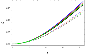
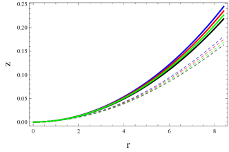
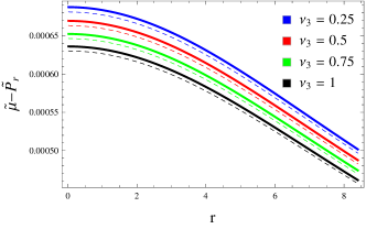
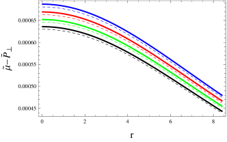
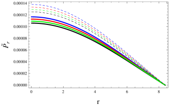
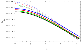
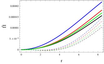
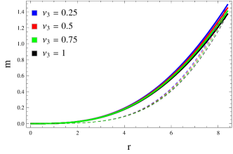
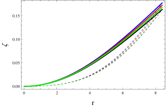
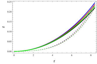
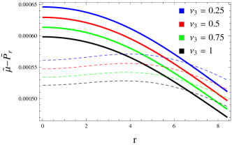
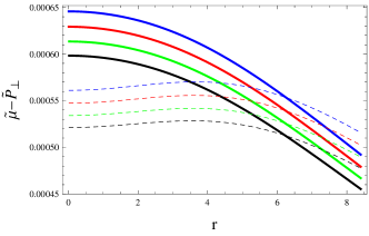
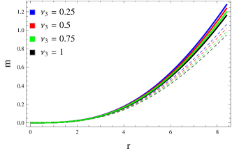
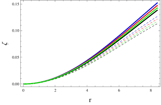
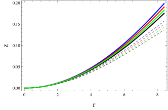
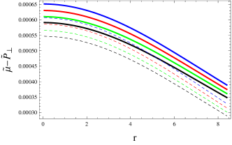
Figure 12 shows increasing trend outwards and in an inverse relation with the model parameter. We utilize Eqs.(25) and (26) to construct the corresponding matter triplet and anisotropy. The variation of these variables with respect to , and is shown in Figure 13, indicating an acceptable profile (see Tables 6 and 7 for numerical values). They show the same behavior as we have found for the first and second models. Figure 14 presents the plots of the mass function, redshift and compactness that are consistent with their acceptable limits. Further, this solution produces less massive interior in comparison with models I and II. The variation of the energy conditions and is shown in Figure 15, demonstrating that our model III is viable. Both criteria of stability (Figure 16) indicate that the developed model is stable for every parametric choice.

7 Conclusions
In this paper, we have formulated different anisotropic extensions of the known isotropic solution through gravitational decoupling for the model . Initially, we have assumed that a sphere is filled with an isotropic fluid that becomes anisotropic after inserting an additional source at the action level. The modified form of the action (1) has then triggered the field equations involving the effects of both seed isotropic as well as additional sources and modified theory. We have then split these equations into two sets through MGD strategy. We have dealt with the unknowns of the first set by choosing Buchdahl anstaz given by
and calculated the triplet through junction conditions at . Moreover, the -sector (22)-(24) comprised four unknowns that needed to be determined. Therefore, we have imposed different constraints on , resulting in three different solutions. We have then added these solutions corresponding to both fluid sources through the parameter and obtained new anisotropic extensions.
We have discussed acceptability conditions such that the resulting solution must be in agrement with them. Such physical characteristics of all the developed models have been interpreted graphically for and . We have observed an acceptable behavior of the matter determinants and anisotropy in each case for all parametric values. The numerical values of the mass function indicates that the second model produces massive interior in comparison to the others. The redshift and compactness factors have also been shown compatible with the experimental data. The dominant energy bounds are satisfied in the region , ensuring the viability of the obtained solutions. Finally, we have noticed that the cracking occurs only in the first model, hence, models II and III are stable.
Morales and Tello-Ortiz [85] extended the Durgapal’s fifth
model to the anisotropic domain through the MGD approach and
obtained the more dense structure in comparison with our developed
solutions. Andrade and Contreras [86] used Tolman IV,
Heintzmann IIa and Durgapal IV as seed solutions, and proposed
different anisotropic extensions by using the definition of the
complexity factor. The anisotropy was also discussed in the interior
of SMC X-1 and Cen X-3 stars from which we found this factor to be
much greater as compared to that obtained in the current setup.
Maurya et al. [87] investigated the possible existence of
compact stars influenced by the electromagnetic field in the
framework of Gauss-Bonnet gravity and determined the exact solutions
to the corresponding field equations in contrast with our work. It
is important to stress here that our models I, II and III are
consistent with [45], [88] and [89],
respectively. All our results reduce to for
.
Data Availability Statement: This manuscript has no
associated data.
References
- [1] Capozziello, S. et al.: Class. Quantum Grav. 25(2008) 085004.
- [2] Nojiri, S. et al.: Phys. Lett. B 681(2009)74.
- [3] de Felice, A. and Tsujikawa, S.: Living Rev. Relativ. 13(2010)3.
- [4] Nojiri, S. and Odintsov, S.D.: Phys. Rep. 505(2011)59.
- [5] Sharif, M. and Kausar, H.R.: J. Cosmol. Astropart. Phys. 07(2011)022.
- [6] Astashenok, A.V., Capozziello, S., Odintsov, S.D. and Oikonomou, V.K.: Phys. Lett. B 816(2021)136222.
- [7] Astashenok, A.V., Capozziello, S. and Odintsov, S.D.: J. Cosmol. Astropart. Phys. 12(2013)040.
- [8] Astashenok, A.V., Capozziello, S. and Odintsov, S.D.: Astrophys. Space Sci. 355(2015)333.
- [9] Astashenok, A.V., Odintsov, S.D. and De la Cruz-Dombriz, A.: Class. Quantum Grav. 34(2017)205008.
- [10] Astashenok, A.V., Capozziello, S., Odintsov, S.D. and Oikonomou, V.K.: Phys. Lett. B 811(2020)135910.
- [11] Astashenok, A.V., Capozziello, S., Odintsov, S.D. and Oikonomou, V.K.: EPL 136(2022)59001.
- [12] Astashenok, A.V., Odintsov, S.D. and Oikonomou, V.K.: Phys. Rev. D 106(2022)124010.
- [13] Bertolami, O. et al.: Phys. Rev. D 75(2007)104016.
- [14] Naseer, T., Sharif, M., Fatima, A. and Manzoor, S.: Chin. J. Phys. 86(2023)350.
- [15] Harko, T. et al.: Phys. Rev. D 84(2011)024020.
- [16] Deng, X.M. and Xie, Y.: Int. J. Theor. Phys. 54(2015)1739.
- [17] Houndjo, M.J.S.: Int. J. Mod. Phys. D 21(2012)1250003.
- [18] Das, A. et al.: Phys. Rev. D 95(2017)124011.
- [19] Singh, K.N. et al.: Phys. Dark Universe 30(2020)100620.
- [20] Maurya, S.K.: Phys. Dark Universe 30(2020)100640.
- [21] Rej, P., Bhar, Piyali. and Govender, M.: Eur. Phys. J. C 81(2021)316.
- [22] Kaur, S., Maurya, S.K., Shukla, S. and Nag, R.: Chin. J. Phys. 77(2022)2854.
- [23] Sharif, M. and Naseer, T.: Eur. Phys. J. Plus 137(2022)1304.
- [24] Sharif, M. and Naseer, T.: Phys. Scr. 98(2023)115012.
- [25] Sharif, M. and Naseer, T.: Ann. Phys. 459(2023)169527.
- [26] Zubair, M., Waheed, S. and Ahmad, Y.: Eur. Phys. J. C 76(2016)444.
- [27] Das, A., Rahaman, F., Guha, B.K. and Ray, S.: Eur. Phys. J. C 76(2016)654.
- [28] Moraes, P.H.R.S., Correa, R.A.C. and Lobato, R.V.: J. Cosmol. Astropart. Phys. 07(2017)029.
- [29] Zaregonbadi, R. et al.: Phys. Rev. D 94(2016)084052.
- [30] Buniy, R.V., Berera, A. and Kephart, T.W.: Phys. Rev. D 73(2006)063529.
- [31] Saadeh, D., Feeney, S.M., Pontzen, A., Peiris, H.V. and McEwen, J.D.: Phys. Rev. Lett. 117(2016)131302.
- [32] Mishra, B., Ray, P.P. and Myrzakulov, R.: Eur. Phys. J. C 79(2019)34.
- [33] Sokolov, A.I.: Sov. Phys.-JETP 52(1980)575.
- [34] Sawyer, R.F.: Phys. Rev. Lett. 29(1972)382.
- [35] Weber, F.: J. Phys. G: Nucl. Part. Phys. 25(1999)R195.
- [36] Schunck, F.E. and Mielke, E.W.: Class. Quantum Grav. 20(2003)R301.
- [37] Rahaman, F., Ray, S., Jafry, A.K. and Chakraborty, K.: Phys. Rev. D 82(2010)104055.
- [38] Maurya, S.K., Mishra, B., Ray, S. and Nag, R.: Chin. Phys. C 46(2022)105105.
- [39] Migkas, K. and Reiprich, T.H.: Astron. Astrophys. 611(2018)A50.
- [40] Migkas, K., Schellenberger, G., Reiprich, T.H., Pacaud, F., Ramos-Ceja, M.E. and Lovisari, L.: Astron. Astrophys. 636(2020)A15.
- [41] Ovalle, J.: Mod. Phys. Lett. A 23(2008)3247.
- [42] Ovalle, J. and Linares, F.: Phys. Rev. D 88(2013)104026.
- [43] Casadio, R., Ovalle, J. and Da Rocha, R.: Class. Quantum Grav. 32(2015)215020.
- [44] Ovalle, J. et al.: Eur. Phys. J. C 78(2018)960.
- [45] Sharif, M. and Sadiq, S.: Eur. Phys. J. C 78(2018)410.
- [46] Sharif, M. and Waseem, A.: Ann. Phys. 405(2019)14.
- [47] Gabbanelli, L., Rincón, Á. and Rubio, C.: Eur. Phys. J. C 78(2018)370.
- [48] Estrada, M. and Tello-Ortiz, F.: Eur. Phys. J. Plus 133(2018)453.
- [49] Hensh, S. and Stuchlík, Z.: Eur. Phys. J. C 79(2019)834.
- [50] Sharif, M. and Ama-Tul-Mughani, Q.: Mod. Phys. Lett. A 35(2020)2050091.
- [51] Sharif, M. and Naseer, T.: Chin. J. Phys. 73(2021)179.
- [52] Sharif, M. and Naseer, T.: Int. J. Mod. Phys. D 31(2022)2240017.
- [53] Sharif, M. and Naseer, T.: Indian J. Phys. 96(2022)4373.
- [54] Naseer, T. and Sharif, M.: Universe 8(2022)62.
- [55] Ashmita, Sarkar, P. and Das, P.K.: Int. J. Mod. Phys. D 31(2022)2250120.
- [56] Kaur, S., Maurya, S.K., Shukla, S. and Nag, R.: Chin. J. Phys. 77(2022)2854.
- [57] Sharif, M. and Naseer, T.: Class. Quantum Grav. 40(2023)035009.
- [58] Naseer, T. and Sharif, M.: Fortschr. Phys. 71(2023)2300004.
- [59] Maurya, S.K. and Tello-Ortiz, F.: Phys. Dark Universe 27(2020)100442.
- [60] Maurya, S.K., Mishra, B., Ray, S. and Nag, R.: Chin. Phys. C 46(2022)105105.
- [61] Buchdahl, H.A.: Phys. Rev. 116(1959)1027.
- [62] Vaidya, P.C. and Tikekar, R.: J. Astrophys. Astro. 3(1982)325.
- [63] Kumar, J., Prasad, A.K., Maurya, S.K. and Banerjee, A.: Eur. Phys. J. C 78(2018)540.
- [64] Sharma, R., Karmakar, S. and Mukherjee, S.: Int. J. Mod. Phys. D 15(2006)405.
- [65] Maurya, S.K. et al.: Phys. Rev. D 99(2019)044029.
- [66] Singh, K.N., Pant, N. and Pradhan, N.: Astrophys. Space Sci. 361(2016)173.
- [67] Maurya, S.K., Banerjee, A. and Tello-Ortiz, F.: Phys. Dark Universe 27(2020)100438.
- [68] Maurya, S.K., Singh, K.N., Govender, M. and Ray, S.: Fortschr. Phys. 71(2023)2300023.
- [69] Gangopadhyay, T., Ray, S., Xiang-Dong, L., Jishnu, D. and Mira, D.: Mon. Not. R. Astron. Soc. 431(2013)3216.
- [70] Delgaty, M.S.R. and Lake, K.: Comput. Phys. Commun. 115(1998)395.
- [71] Ivanov, B.V.: Eur. Phys. J. C 77(2017)738.
- [72] Sharif, M. and Naseer, T.: Phys. Dark Universe 42(2023)101324.
- [73] Sharif, M. and Naseer, T.: Chin. J. Phys. 86(2023)596.
- [74] Sharif, M. and Naseer, T.: Gen. Relativ. Gravit. 55(2023)87.
- [75] Naseer, T. et al.: Mod. Phys. Lett. A 39(2024)2450048
- [76] Feng, Y. et al.: Chin. J. Phys. 90(2024)372.
- [77] Feng, Y. et al.: Phys. Scr. 99(2024)085034.
- [78] Naseer, T. and Sharif, M.: Chin. J. Phys. 88(2024)10.
- [79] Ivanov, B.V.: Phys. Rev. D 65(2002)104011.
- [80] Abreu, H., Hernandez, H. and Nunez, L.A.: Class. Quantum Grav. 24(2007)4631.
- [81] Herrera, L.: Phys. Lett. A 165(1992)206.
- [82] Heras, C.L. and León, P.: Fortschr. Phys. 66(2018)1800036.
- [83] Graterol, R.P.: Eur. Phys. J. Plus 133(2018)244.
- [84] Contreras, E. and Bargueño, P.: Class. Quantum Grav. 36(2019)215009.
- [85] Morales, E. and Tello-Ortiz, F.: Eur. Phys. J. C 78(2018)841.
- [86] Andrade, J. and Contreras, E.: Eur. Phys. J. C 81(2021)889.
- [87] Maurya, S.K. et al.: Eur. Phys. J. C 82(2022)552.
- [88] Azmat, H. and Zubair M.: Eur. Phys. J. Plus 136(2021)112.
- [89] Al Hadhrami, M. et al.: Pramana 97(2022)13.